![]()
![]()
![]() \SetWatermarkAngle0
\SetWatermarkAngle0
Bidirectional Evaluation with Direct Manipulation
Abstract.
We present an evaluation update (or simply, update) algorithm for a full-featured functional programming language, which synthesizes program changes based on output changes. Intuitively, the update algorithm retraces the steps of the original evaluation, rewriting the program as needed to reconcile differences between the original and updated output values. Our approach, furthermore, allows expert users to define custom lenses that augment the update algorithm with more advanced or domain-specific program updates.
To demonstrate the utility of evaluation update, we implement the algorithm in Sketch-n-Sketch, a novel direct manipulation programming system for generating HTML documents. In Sketch-n-Sketch, the user writes an ML-style functional program to generate HTML output. When the user directly manipulates the output using a graphical user interface, the update algorithm reconciles the changes. We evaluate bidirectional evaluation in Sketch-n-Sketch by authoring ten examples comprising approximately 1400 lines of code in total. These examples demonstrate how a variety of HTML documents and applications can be developed and edited interactively in Sketch-n-Sketch, mitigating the tedious edit-run-view cycle in traditional programming environments.
1. Introduction
Expert programmers often choose to write programs to generate digital objects that might otherwise be created in graphical user interfaces (GUIs) using direct manipulation (Shneiderman, 1983; Hutchins et al., 1985), because GUIs typically lack powerful mechanisms for abstraction and reuse. To name just a few example languages and libraries, LaTeX is particularly popular for generating documents; JavaScript, Ruby, and Elm for web applications; Processing and p5.js (http://p5js.org/) for graphic designs; LaTeX and Slideshow (Findler and Flatt, 2006) for slide-based presentations; and D3 (Bostock et al., 2011) for data visualizations.
The benefits of programming, however, come at a steep cost: to change the output of a program, the user must edit the source code, run it again, and view the new output, often repeating this loop ad nauseaum. Effort wasted in this way is particularly galling when successive program changes—and the resulting output changes—are small and narrow in scope. Ideally, the user would “directly manipulate” the program output, and the system would run the program “in reverse” to synthesize necessary program repairs.
Prior Approaches
Two primary approaches help address the goal to run programs in reverse. In bidirectional programming languages (Foster et al., 2007), data transformations are defined as lenses, in which a -function for forward-evaluation is paired with a -function for backward-evaluation—when the output of is changed, specifies how to change the input. A bidirectional language provides a set of domain-specific lens primitives, from which programmers mold desired transformations using lens combinators. Lenses have proven to be effective for defining bidirectional transformations in a variety of domains—including structured data (relational tables), semi-structured data (trees), unstructured data (strings), and graphs. Nevertheless, lenses are not a solution for automatically reversing the computation of an arbitrary program—data and code—written in a general-purpose functional language (Limitation A).
Another approach, developed by Chugh et al. (2016), aims to reverse arbitrary programs as follows. First, the interpreter records value traces to track the provenance of how values are computed. Then, when the user makes small changes to the output, updated value-trace equations are solved in order to synthesize repairs to the program. Although a useful step, this approach suffers several limitations. First, the formulation supports tracing and updates for numeric values, but not for other types of simple or more complex values (Limitation B). Second, the formulation provides no way for expert users to customize the behavior of the algorithm (Limitation C). This is a significant limitation in practice, because no single update algorithm for arbitrary programs can work well in all use cases. Furthermore, even if extended to address the aforementioned limitations, the approach requires that all computations be traced even if many (or most) values are not updated by the user. For a large program where the subset of values that are directly manipulated becomes a small fraction, the space overhead of this approach could become a bottleneck, as is often the case for systems that record execution traces, such as omniscient debuggers (Pothier et al., 2007) and query-based debuggers (Ko and Myers, 2008) (Limitation D).
Our Approach: Bidirectional Evaluation
In contrast to prior approaches, we propose a notion called bidirectional evaluation for programs in a full-featured, general-purpose functional programming language. In addition to a standard evaluation relation that evaluates expression to value , we define an evaluation update (or simply, update) relation that, given an expected value , rewrites the original expression to . Evaluation update proceeds by comparing the original output value with the goal , and synthesizing repairs to such that, ideally, the new program evaluates to . Evaluation update is defined for arbitrary expressions producing arbitrary types of values , thus addressing Limitations A and B, respectively. Our approach relies on standard, uninstrumented evaluation; we re-evaluate expressions as needed during update. This approach trades time for space, thus addressing Limitation D.
Furthermore, we allow expert users to define custom lenses that augment the
update algorithm with more advanced or domain-specific program updates, thus
addressing Limitation C.
In particular, in place of an ordinary function application
, the program can define a
lens application
,
in which case, the update algorithm uses the designated update
function to help compute a new expression
to replace the argument .
Our Implementation: Direct Manipulation Programming for HTML
We implement bidirectional evaluation within Sketch-n-Sketch (Chugh et al., 2016), an interactive programming system for developing and editing graphical objects. In the new system, the user writes a program in a functional, ML-style language to generate HTML output. When the user directly manipulates the output using a graphical user interface, the update algorithm synthesizes repairs to reconcile the changes. Our user interface provides a lightweight mechanism for previewing and choosing a solution when there is ambiguity, inherent to the setting of a general-purpose language.
We used our new version of Sketch-n-Sketch to author 10 examples comprising approximately 1400 lines in total, demonstrating how a variety of interactive documents and applications—web pages, Markdown-to-HTML translators, scalable recipe editors, and what-you-see-is-what-you-get (WYSIWYG) LaTeX editors—can be programmed in a way that allows direct manipulation changes to propagate automatically back to the program. Moreover, our prototype implementation typically synthesizes program repairs for our examples in between 0 and 2 seconds, which suggests that our techniques can be further developed and optimized for more full-featured, interactive settings.
Contributions and Outline
To summarize, this paper provides the following contributions.
-
(1)
We present the notion of bidirectional evaluation, where arbitrary programs in a general-purpose functional language can be run in reverse in order to produce useful edits to the program. To achieve this, we define an evaluation update algorithm that—compared to typical evaluation—receives an expected output value as an argument, used to synthesize repairs to the expression such that it computes the expected value. (§ 3.1)
-
(2)
We develop an approach for custom update lenses that allow experts to augment evaluation update with more advanced or domain-specific program updates. To improve the utility of the “built-in” evaluation update algorithm, we show how to define custom update lenses for several common functional programming patterns. (§ 3.2)
-
(3)
We implement our approach within Sketch-n-Sketch; the new system is available on the web at http://ravichugh.github.io/sketch-n-sketch/. Our implementation includes optimizations to make the update algorithm perform well in practice, as well as programming conveniences found in practical, ML-style functional languages. Our examples and experiments demonstrate that the expressiveness and performance of bidirectional evaluation in Sketch-n-Sketch helps integrate the benefits of programmatic and direct manipulation. (§ 4 and § 5)
In the remainder of the paper, unqualified references to Sketch-n-Sketch refer to the new system. Next, in § 2, we describe an overview example to introduce the workflow enabled by bidirectional evaluation in Sketch-n-Sketch, before describing the approach in detail.
2. Overview
Consider the task for a web developer to implement an HTML table that displays each of the United States along with their capital cities. In Sketch-n-Sketch, the developer first writes a program in Leo—a functional language that resembles Elm (http://elm-lang.org/)—that generates a prototype. The initial programming effort required to encode all intended data and presentation constraints is similar to when using traditional text-based programming environments. Afterwards, however, Sketch-n-Sketch allows the developer to: (a) edit the data and design parameters through direct manipulation interactions; and (b) add rows to the table through a custom, library-defined user interface. Sketch-n-Sketch synthesizes program repairs based on these interactions.
2.1. Initial Programming Effort
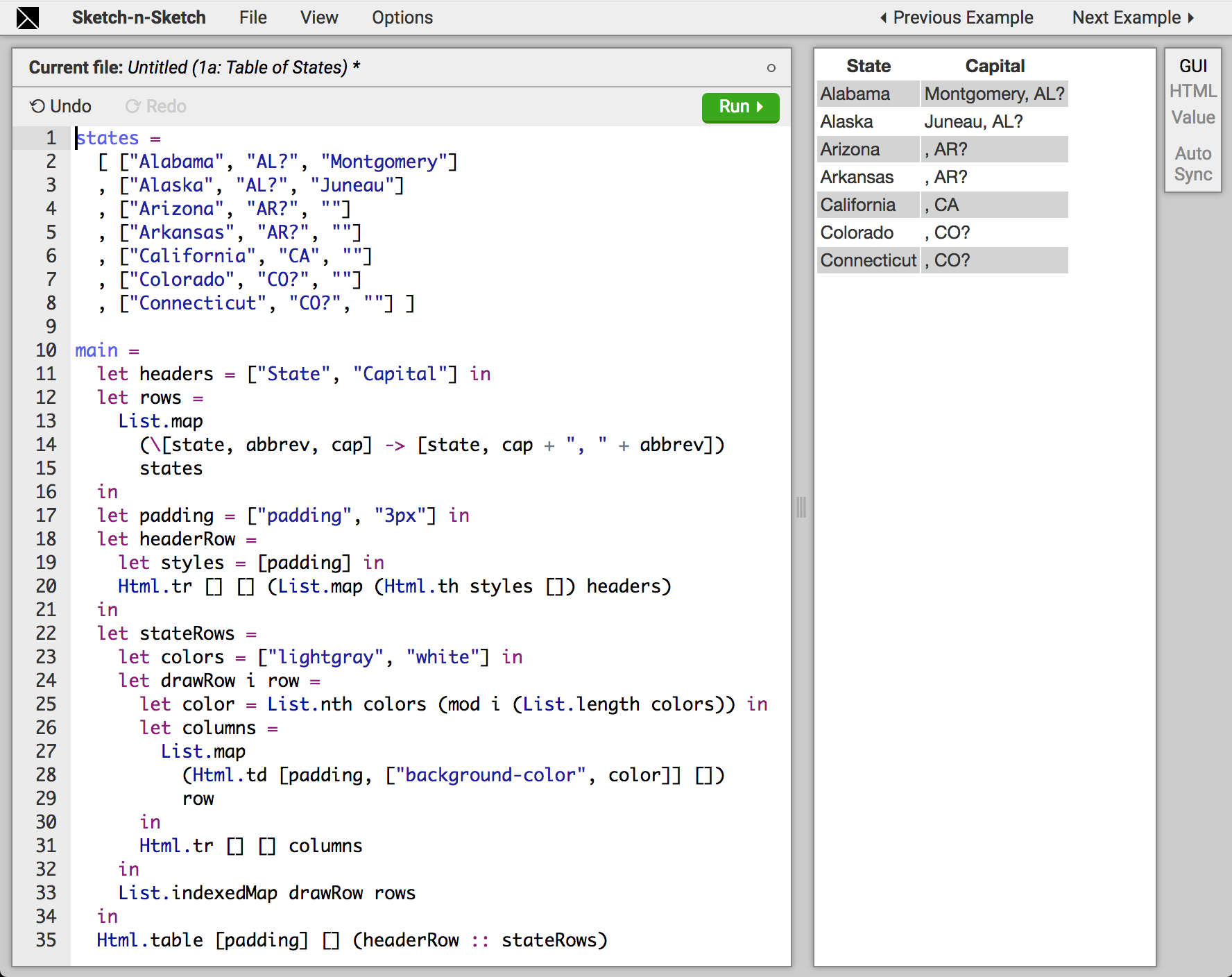
Figure 1 shows a Leo program
to generate an initial prototype.
In the following, we typeset string literals in the program with
typewriter font (e.g. "California") and strings in the HTML output with
slanted font (e.g. "California").
Lines 1 through 8 define the table data; each element of
states is a three-element list, containing a state name, two-letter
abbreviation, and capital city.
For now, the data is incomplete—unknown abbreviations and capitals are
marked with question marks (e.g. "AL?" on lines 1–2) and
empty strings (i.e. "" on lines 4–8).
The main definition, starting on line 10, generates the output HTML
table.
First, the developer decides to produce two output columns: one for the state
name (e.g. "Alabama"); and one for its capital city,
concatenated with the state abbreviation (e.g. "Montgomery, AL").
The headers definition (line 11) contains text for
the header row, and the rows definition (lines 12–15)
contains the text to display in subsequent rows by mapping
each three-element list
[state, abbrev, cap] in states to the two-element list
[state, cap + ", " + abbrev].
The headerRow definition (lines 18–20) uses library
functions Html.tr and Html.th to generate table row and
header elements, respectively, for the top of the table.
These Html functions take three arguments—a list of HTML
style attributes, a list of additional HTML attributes, and a list of HTML
child nodes—and produce straightforward encodings of HTML values to be
rendered.
The stateRows definition (lines 22–33) generates the
remaining rows of the table.
The colors list (line 23) defines two initial
colors—"lightgray" and "white"—and
the expression (line 25) chooses one of these colors based on the parity
of row index i (received as a parameter from the
List.indexedMap library function).
The columns definition (lines 26–29) places the text
for each state and its capital city—in a two-element list
row—inside Html.td elements, which comprise a row
built from the Html.tr expression (line 31).
Lastly, the expression on line 35 builds the overall Html.table
element comprising headerRows and stateRows.
The output Leo value is translated to HTML in a straightforward manner
and rendered graphically in the
right half of Sketch-n-Sketch, as shown in
Figure 1.
2.2. Direct Manipulation of Output Text
Having encoded the intended programmatic relationships for the data and design of the table, next the developer wants to correct the missing data (lines 2–8). In Sketch-n-Sketch, the developer can edit text directly in the graphical user interface that displays the output (the right half of the editor). The interactions described in this subsection, and the following ones, can be viewed in screencast videos, available on the web.
Computing and Displaying Program Updates
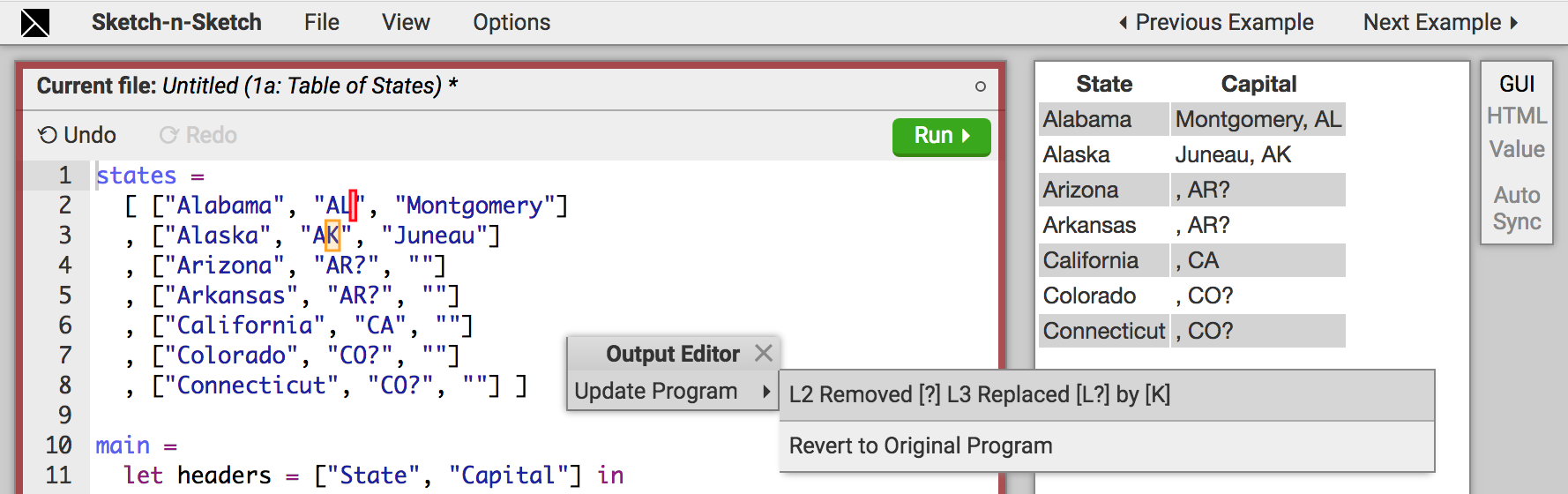
Figure 2 shows an example of how the developer edits the data in the program through the graphical user interface interface; the screenshot shows the editor state after the following sequence of user actions.
First, in the first state row of the output table, the user deletes the question mark after "AL" in the string ", AL?". Next, in the second row, the user replaces the string "AL?" with "AK". As soon as the user begins editing the output table, Sketch-n-Sketch detects that the program output is no longer synchronized with the program. As a result, Sketch-n-Sketch highlights the code box with a red border and displays a pop-up window with a menu item labeled Update Program.
When the user hovers over Update Program, Sketch-n-Sketch runs the evaluation update algorithm to synthesize a repaired program that, when re-evaluated, generates the same result as the directly manipulated output. In this case, the algorithm computes one solution that, along with an option for reverting the changes, is displayed in a nested menu to the right of Update Program. The screenshot in Figure 2 captures the editor state when the user hovers over the first item in the nested menu, at which point Sketch-n-Sketch displays a preview of the updated program (resp. output) directly in the left (resp. right) pane. The caption "L2 Removed [?] L3 Replaced [L?] by [K]" summarizes the string differences, on lines 2 and 3, between the original and updated program text. These differences are highlighted in red and orange in the code box to further help communicate the proposed changes to the user. In this case, the new program matches the user’s expectations, so the user clicks the menu item (not shown in the screenshot) to confirm the update, returning the program and output to a synchronized state.
Ambiguity
Whereas each of the previous output changes resulted in a single solution,
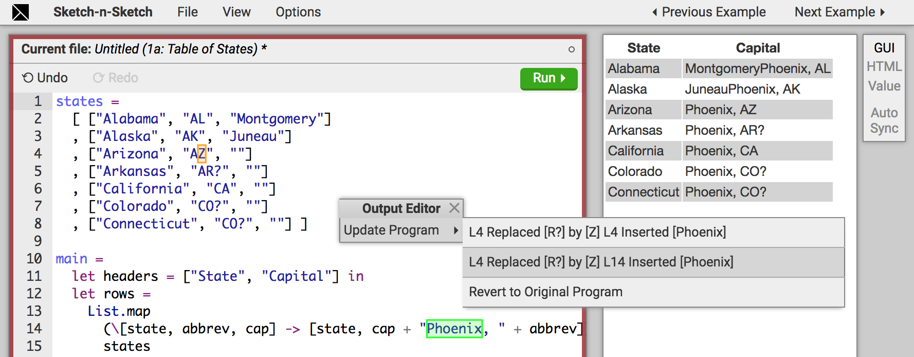
Figure 3 shows a change that leads to multiple.
In the third row, the user replaces ", AR?" with
"Phoenix, AZ".
When the Update Program menu item appears and is hovered, two solutions
are displayed (in addition to the option to revert the changes).
The screenshot in Figure 3 captures the editor state
when the second solution is hovered.
Both solutions replace "AR?" on line 4 with "AZ", as desired, but
the second solution inserts "Phoenix" as a prefix to the ", "
separator string used in the concatenation on line 14.
By viewing the preview of the output—with "Phoenix" appearing
in all rows—the user quickly determines that this change, though consistent
with the output edit, is undesirable.
So, the user hovers and selects the first option (not shown in the screenshot).
Wanting the separator string on line 14 always to remain constant,
the developer edits the source code to wrap the string "", "" in a
call to Update.freeze (not shown), which instructs Sketch-n-Sketch
never to change this expression when computing program updates.
Browser Conveniences for Navigating Output Text
The user fills in missing data for the remaining rows directly in the output pane. Having frozen the separator string already, none of these changes lead to ambiguity. During these interactions, the user benefits from text-editing features built-in to the browser—using the Tab key to advance to subsequent columns and rows, and arrow keys to navigate the text cursor within the selected cell—which make it yet more convenient to specify these changes in the graphical user interface rather than in the source code editor.
2.3. Direct Manipulation with DOM Inspector
Having corrected the table data (as shown in Figure 4), next the developer experiments with different styles. Sketch-n-Sketch allows the developer to use the existing Developer Tools provided by modern browsers to inspect and modify arbitrary elements and attributes in the DOM (i.e. the HTML output of the program); these changes are used to trigger the update algorithm.
Browser Conveniences for Editing Styles
Suppose the user wants to try out different colors for alternating rows, to
replace the colors on line 23.
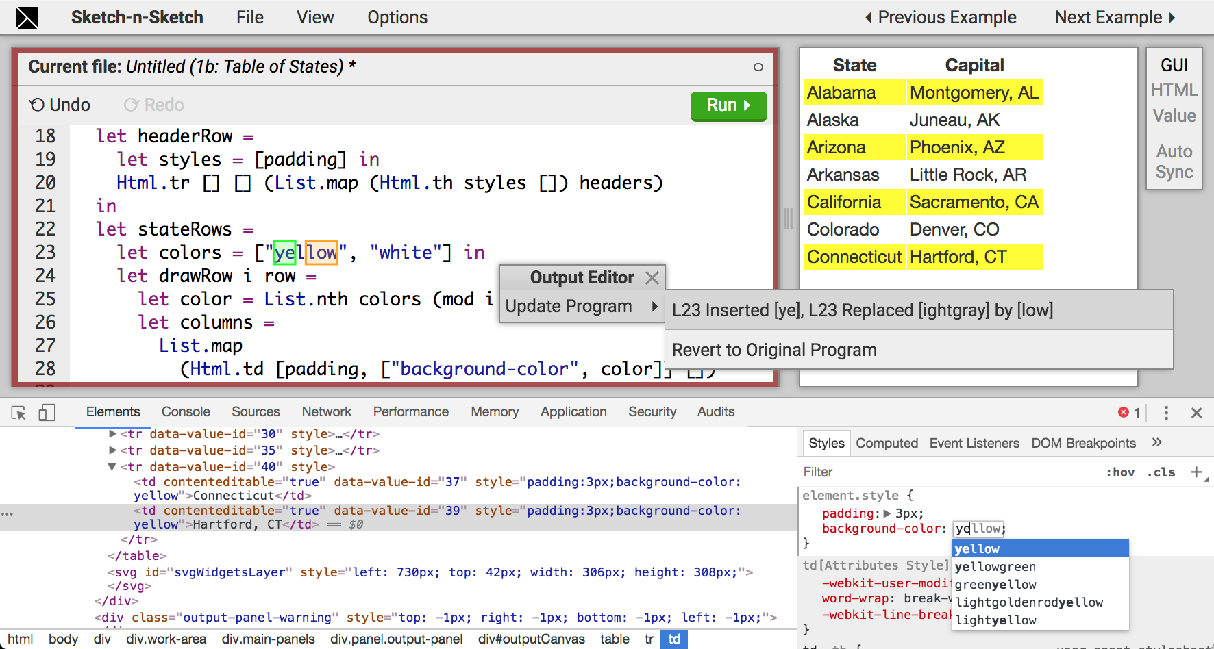
Figure 4 shows how the user can affect such
changes.
First, the user right-clicks the "Hartford, CT" cell and selects
Inspect from the browser’s pop-up menu.
As a result, a Developer Tools pane appears at the bottom of
editor (as shown in the screenshot), with the selected cell in focus in the
DOM Element Inspector.
The rightmost panel provides a Styles Editor,
which the developer can use to
change the background-color from the initial lightgray color.
The developer starts typing ye and, then, using
the built-in conveniences provided by the Styles Editor for
changing color
values—a dropdown menu of related colors, equipped with tab completion and
previews—decides to try the color yellow.
As with the text changes before, Sketch-n-Sketch detects that the output is no longer synchronized with the program, and so displays the Update Program menu. The screenshot in Figure 4 captures the editor state when the user hovers the single solution, which replaces "lightgray" on line 23 with "yellow" to reconcile the change. In the result of this new program, the color of all cells in alternating rows are changed, not just the one cell directly manipulated.
Automatic Synchronization
The developer wants to experiment with colors, but manually hovering and clicking the Update Program menu will be tedious when trying several options. So, the developer clicks the button labeled Auto Sync in the right toolbar. Now whenever the output is changed, the program update algorithm is automatically run after a delay—1000ms by default, but this choice can be configured by the program. When there is a single solution, it is applied automatically. Thus, the developer can try several colors in the DOM Inspector in rapid fashion, viewing how the change propagates (almost) immediately to the entire table.
Small Updates
Next, the developer wishes to add a background color to headerRow, whose
styles list on line 19 does not include a color.
The following interactions are not depicted in screenshots, but they
are in the accompanying videos.
After selecting the first column of the header row in the browser
DOM Inspector (either by right-clicking, or using the browser’s
built-in Inspect cursor), the
developer, again, uses the Styles Editor,
which provides an easy way (with a mouse
click or Enter key press) to add a new attribute.
The user adds
a new background-color attribute set to the value orange,
and the corresponding program update adds the pair
[ "background-color", "orange" ] to the styles
list on line 19.
Unlike all of the local updates, described above, which replaced only
constant literals in the program with new ones, this solution includes
a structural update that alters the structure of the abstract syntax tree.
We call this structural update pretty local because the only change to the
structure is inserting a new literal at a leaf of the AST, i.e. inside another
list literal.
In our experience (§ 5), even just “small” program
updates—local and pretty local—enable a variety of desirable interactions.
2.4. Direct Manipulation with Custom User Interfaces
What about adding a new row with columns "Delaware" and
"Dover, DE" to the bottom of the output table?
The desired program repair is to add a new three-element list
[ "Delaware", "DE", "Dover" ].
to the end of the states list.
As we will explain in § 3, our algorithm does not
automatically perform the complex reasoning required—pushing
the newly inserted value [ "DE", "Dover, DE" ]
back through the call to List.map on line 13 of
Figure 3—to produce the desired program repair.
User-Defined Program Updates with Lenses
For situations like this,
Sketch-n-Sketch provides users (or library writers) a
mechanism to define a custom lens that augments a
“bare” function with a second update function that defines the
“reverse semantics” for the bare function.
Using lenses, the expert user can define a module called
TableWithButtons—which performs more advanced evaluation update
than for basic List.map—to serve as a
drop-in replacement for the basic table-constructing functions in the
Html library.
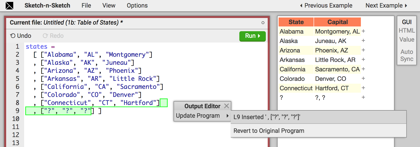
Figure 5 shows how, using this library, the user can click a
button (labeled "+") to indicate that a new row should be added
at that position.
Suppose the user clicks the button next to the "Connecticut" row, hovers
Update Program, and then hovers the single solution (as shown in the
screenshot).
The resulting program
adds a dummy row on line 9 in the
states list, which can later be filled in through the basic direct
manipulation text interactions as before.
Thus, by using lenses to augment the functionality of the built-in
update algorithm, expert users and library writers can implement custom user
interface features for manipulating the particular bidirectional functional
documents under construction.
3. LittleLeo: A Bidirectional Functional Programming Language
In this section, we present the syntax and bidirectional evaluation semantics for LittleLeo, a lambda-calculus that models the Leo language supported in our implementation.111 LittleLeo is a backronym for “a Little language extended with Lenses, Eval, Objects, and other features.”
Syntax
The syntax of LittleLeo is defined in Figure 6. Constants include numbers , booleans , strings , the empty list [], the empty record {}, and primitive operators. The operators updateApp, diff, and merge facilitate the definition of custom lenses, which will be presented after basic evaluation update. Values include constants, closures where the environment binds free variables in the body of the function , and lists and records with multiple components.
The definition of expression forms is spread across three lines: those on the first two lines are standard—constants , variables , function application , list construction , record extension , record field projection , (simple and recursive) let-bindings , conditionals , and case expressions ; and those on the third line are specific to the definition of custom update functions (discussed in § 3.2).
3.1. Bidirectional Evaluation
Evaluation Evaluation Update
Figure 7, Figure 8, and Figure 9 define the bidirectional evaluation semantics for LittleLeo; the big-step evaluation rules (prefixed “E-”) are standard, while the evaluation update (or simply, update) rules (prefixed “U-”) are novel.222 By analogy to bidirectional type checking (Pierce and Turner, 2000; Chlipala et al., 2005), evaluation may be thought of as “value synthesis” and evaluation update as “value checking.” We refer to an environment-expression pair as a program.
The evaluation update judgement states that “when updating its output value to , the program updates to .” The parentheses are for clarity; we typically omit them. When only the expression (resp. environment) changes, we sometimes say “the expression (resp. environment) updates to a new expression (resp. environment).” We sometimes say “push (or changes to ) back to ” in reference to evaluation update. The judgement does not refer to the original value from forward-evaluation; if needed by a premise of an update rule, it is re-computed. Update rules come in three varieties: replacement rules overwrite values (base constants and closures) in the program with new ones; primitive rules define how to update operations on base values, lists, and dictionaries; and propagation rules carry the effects of replacement and primitive rules to the rest of the program (through variables, function calls, conditionals, etc.).
3.1.1. Replacement Rules
There are two axioms, for replacing values. The rule U-Const says that, when updating its output value to , the expression updates to ; the environment remains unchanged. The rule U-Fun says that, when updating its output value to the closure , the program updates to . Although directly updating closures in the output of a program will, perhaps, be less common than other types of values, this rule is nevertheless crucial for “receiving” changes propagated from elsewhere in the program.
3.1.2. Primitive Rules for Base Values
How to update primitive operations may vary in different deployments of bidirectional evaluation. The replacement and propagation rules are agnostic to these choices. Figure 8 shows several simple primitive rules, which we find useful in practice. For example, there are two update rules, U-Plus-1 and U-Plus-2, which, respectively, re-evaluate the left or right operand ( or ) to a number ( or and then push back the updated difference ( or ) entirely to that operand. Because there are two update rules, there are two valid program updates for addition expressions.
3.1.3. Propagation Rules
How to update variables and variable binding forms is the heart of our formulation; they are what allow changes to values at the leaves of the program to flow throughout the program. To simplify the presentation, the evaluation and update rules for let-bindings and function calls assume only variable patterns rather than arbitrary ones, as in our implementation.
Variables
When U-Var updates the output of to , the environment updates to which is like the original except that is bound to the new value ; the expression remains unchanged.
Let-Bindings
Like E-Let, the first premise of U-Let evaluates the expression to a value , to be bound to and added to when subsequently considering the expression body . Dual to E-Let—which, in the new environment, evaluates to a value —the second premise of U-Let pushes back the expected value , producing a (potentially updated) expression body and (potentially updated) environment that is structurally equivalent to the original environment (their domains are equal). Notice that, to produce this new program, the value bound to may differ from the original value . To discharge this obligation, the third premise pushes back to , producing a (potentially updated) expression and (potentially updated) environment that is structurally equivalent to . Putting these pieces together, the new expression is . What remains is to reconcile and with the original . The rules ensure that and are both structurally equivalent to , but each may have induced updates to one or more bindings in . As demonstrated below, updated bindings may conflict—there may be variables such that and are different. To produce the final environment, the conclusion of U-Let uses an environment merge operation, , discussed next.
Environment, Value, and Expression Merge
The merge operation—used by all rules that update multiple subexpressions—takes two structurally equivalent environments and to merge, as well as several optional arguments: the original environment , and the expressions and that were updated when and were produced. We consider two implementations for this operation.
Definition 3.1 (Conservative Two-Way Merge).
Two-way environment merge , reconciles bindings as follows (the subscript is omitted because the original environment is ignored).
If neither environment updates the binding, or if both update it to the same new value, the first equation adds the new value to the merged environment. Otherwise, the second (resp. third) equation adds the new value from the left environment (resp. from the right environment ) only if does not appear free in (resp. ).
Two-way merge is conservative; if a variable appears free in both expressions, two-way merge requires that it be updated to the same new value in both environments. In other words, all occurrences of an updated variable must be updated consistently for the overall update to succeed. Though restrictive, this would be necessary to ensure that the new program evaluates to the updated value; § 3.1.5 describes a correctness property that depends on the use of two-way merge. In practice, however, we prefer to support interactions where the user can update only a subset of the uses—often just one—of a particular variable. To support this workflow, we propose an alternative way to merge environments.
Definition 3.2 (Optimistic Three-Way Merge).
Three-way environment merge performs three-way value merge on variable bindings as follows (the superscripts and are omitted because these expressions are ignored).
The value merge operation (not shown) recursively traverses the subvalues of three structurally equivalent values, until the rule for base cases—for merging constants—chooses if it differs from (even if and conflict) and otherwise.333 An implementation could, instead, choose to favor updates from the left, or even propagate all combinations of choices. Closure values include expressions, so we also define a three-way expression merge operation (not shown) in similar fashion. Three-way merge is optimistic; it succeeds despite conflicts. As a result, use of three-way merge precludes the correctness property enjoyed by the use of two-way merge. Nevertheless, we expect three-way merge to be the default mode of use in practice and choose it for our implementation (§ 4). In our experience, we find that desirable updates are often produced by this configuration (§ 5).
Example 3.3.
Consider the expression , which evaluates to [ 1, 1 ]. (The rule U-Cons for updating lists, discussed in detail below, updates the list element expressions and then merges the updated environments.) If updated to, say, [ 1, 2 ] or [ 0, 2 ], the U-Let, U-Cons, and U-Var rules—together with the right-biased, three-way merge—combine to update the program to , which, when evaluated, produces [ 2, 2 ]. Using two-way merge, however, update fails to produce a solution.
Function Application
Having seen the basic approach to propagating changes through environments, we now turn to the rule U-App for function application (Figure 7).444 Consistent with the standard rewriting of to , U-Let is derivable from U-Fun and U-App. The approach is like that of U-Let, extended now to also deal with the closure through which a value flows. The first two premises re-evaluate the function to a closure and the argument to a value . The third premise pushes the updated value back through the function call, specifically, through the function body , where the closure environment is extended with the binding . This produces a new function body and a new, structurally equivalent environment with a new argument value . Three terms must be reconciled with the original program: the function environment (), the function body (), and the function argument (). The fourth premise pushes the first and second terms, in the form of the closure , back to the original function expression ; the result is a new program . The fifth premise pushes the third term, , back to the original argument expression ; the result is a new program . Environment merge is used to combine and , and the updated function application expression is .
Control-Flow
Rule U-If-True (Figure 7) pushes the updated value back to the then-branch, assuming that the same branch will be taken by the new program. Rule U-If-False (not shown) does the same for the else-branch. Notice that new environment is the result of merging the original environment with the environment produced when updating the then-branch. The conservative two-way merge would ensure that all free variables of must be bound to the same values in as in ; thus, the guard expression in the new program would evaluate to the same boolean value. As discussed above, however, our implementation is configured to use three-way merge. Indeed, several of our example use cases for direct manipulation interaction (§ 5) purposely alter control-flow, e.g. because of a change to a boolean flag.
Example 3.4.
Consider the expression which evaluates to 1. If the user updates the value to 2, the change will be pushed back to the then-branch, and then back through the variable use to the function argument. If using two-way merge, the update would fail because the updated variable, , is free in the guard expression. If using three-way merge, the updated expression would be , which, when evaluated, takes the else-branch and produces 3 instead of 2.
Expression Freeze
The update rules are applied “automatically” to all relevant (sub)expressions when trying to reconcile the program with a new output value. The expression is semantically a no-op (E-Freeze in Figure 7) but is one simple way to control the update algorithm, by requiring that the expression and values it computes remain unaltered (U-Freeze in Figure 7).
3.1.4. Primitive Rules for Lists and Dictionaries
We have considered replacement, primitive, and propagation rules for a core language with base values. We now discuss primitive rules for updating data structures in LittleLeo, namely, lists and dictionaries.
List Construction
Figure 9 shows a standard evaluation rule (E-Cons) for list construction, and a corresponding update rule (U-Cons) that propagates changes to the head (resp. tail) value back to the head (resp. tail) expression. Notice that these rules preserve the structure of existing cons expressions; we choose not to include structure-changing rules that add and remove cons expressions because of the amount of ambiguity they would introduce.
List Literals: Pretty Local Updates
The primitive rules presented in Figure 8 update expressions without altering their structure. Even rules such as U-Lt, which update the operator, preserve the arity of the application. This approach ensures a predictable class of “small” changes, but the same restriction applied to data structures would preclude seemingly benign changes—e.g. updating the empty list expression [] with new value [ 1 ].
Our design includes the rule U-List (Figure 9) to allow insertion and deletion inside list literals that appear in the program—we refer to this form of structural change as pretty local to emphasize its limited effect on the program structure. We write as syntactic sugar for the nested list construction expression that terminates with the empty list. The helper procedure takes the original and updated list values and computes a value difference (a “delta”), in this case, a sequence of list difference operations—, , , or . Our implementation of uses a dynamic programming approach that, intuitively, attempts to preserve as many contiguous sequences from the original list as possible. We reuse the syntax of the evaluation update judgement for one that pushes back value differences (rather than just values), with the subscript to help distinguish them: computes the list literal that results from traversing the original list literal and the difference operations, keeping, inserting, deleting, or updating expressions as dictated by the difference.
String, Records, and Dictionaries
Evaluation rules (not shown) for string concatenation , record literals , and record extension are standard. Dictionary values are built using primitive operators empty, get, insert, remove, and fromList. Update rules for dictionaries work much the same way as those for lists, based on dictionary difference operations that are analogous to the list difference operations, discussed above. Update rules for records and record extension are also similar, except that there are no insertions or deletions. Update rules for concatenating strings and appending lists require a more nuanced approach, as explained in § 3.2.
3.1.5. Correctness
We now describe two correctness properties that relate evaluation and evaluation update. The first correctness property is straightforward.
Theorem 3.5 (EvalUpdate).
If , then . (i.e. If the program evaluates to , pushing the same value back to the program does not change the program.)
Next, we define the notation (with a check mark above the right arrow) to refer to the conservative version of update that uses two-way environment merge. The second correctness property pertains only to this version.
Theorem 3.6 (Conservative UpdateEval).
If , then . (i.e. If, when using two-way merge, pushing back to the program produces , the new program evaluates to the updated value).
Recall that the two challenges for correctness of update are when variables uses are not updated consistently and when control-flow decisions deviate from their original directions. The two-way environment merge operator is defined and used precisely to curb these situations. A detailed proof sketch is available in Supplementary Appendices (Mayer et al., 2018).
3.2. Customizing Evaluation Update
Because of the inherent expressiveness of the language, evaluation update cannot provide all possible intended behaviors that users may desire. Consider the common evaluation and update pattern, below, that is not well-handled by the update algorithm.
The operation computes the following alignment between the original and updated values: that and have been updated to and , and new values and have been inserted after (the updated versions of) and . What would be desirable is an updated program of the form indicated above, where , , and are updated because of the two updated function calls and , and where the synthesized expressions are are passed to the function , ideally producing the inserted values and .
Unfortunately, the evaluation update approach described so far
cannot synthesize repairs of the desired form above.
To understand why, consider the standard definition of map:
letrec map f list = case list of [] -> []; x::xs -> f x :: map f xs
Notice that the original list value
is constructed
completely within the body of map: non-empty (cons) nodes are created in
the list x::xs branch and the empty node is created in the
list [] branch.
To reconcile the updated list,
would have to be inserted into the empty list [] in map,
and would have to be inserted into the cons-node.
Besides the fact that we disallow structural updates anywhere but E-List
(cf. the “List Literals: Pretty Local Updates” discussion in
§ 3.1), such
changes are not desirable—the new cons-node would not
be the result of applying f to anything; it would end up inserting the same
element in between all elements in the output; and we want the definition
of map, a library function, to be frozen anyway.
In short, the evaluation update has no means to provide simultaneous reasoning about structural changes to list values and computations they pass through. This is one simple programming pattern not handled well; surely there are many others.
3.2.1. User-Defined Update Functions
Instead of providing built-in support for updating map and
other common building blocks, we expose an API for users (or
libraries) to customize evaluation update.
Specifically, when a “bare” function is called, the program may
optionally provide a second “update” function that specifies how
to push new argument values back to the call.
A pair comprising bare and update functions forms a
lens (Foster et al., 2007),
specified in LittleLeo as a record with the following type
(written in comments starting with ‘--’ because, currently, our presentation and implementation do
not include types):
-- type alias Lens a b = -- { apply: a -> b, update: {input: a, outputNew: b} -> {values: List a} }
In lieu of types,
the expression syntactically marks
the function application as a lens application.
The E-Lens rule (Figure 10)
projects the field of the lens
argument and then applies it to the argument .
To push a new value back to the lens application
, the U-Lens rule uses the
function of the lens.
The function argument is re-evaluated to
and, together with the new output , is passed to the
function.
Each value in the values list of results is pushed back to
the expression argument and then used as the argument of the updated
function call expression.
Because the lens mechanism in LittleLeo is intended to provide a way to
customize the built-in update algorithm, we expose several internal
operators—updateApp, diff, and merge
(Figure 6)—that custom update functions can refer to.
We will explain the semantics of these operations (Figure 10)
as they arise in the discussion below.
3.2.2. Example Lenses
Before defining a custom lens for list map, we start with a simpler example:
mapping a “MaybeOne” value, encoded as a list with either zero or one elements.
Maybe Map
-- type alias MaybeOne a = List a-- maybeMapSimple : (a -> b) -> MaybeOne a -> MaybeOne b maybeMapSimple f mx = case mx of [] -> [] [x] -> [f x]-- maybeMapLens : a -> Lens (a -> b, MaybeOne a) (MaybeOne b) maybeMapLens default = { apply (f, mx) = Update.freeze maybeMapSimple f mx , update {input = (f, mx), outputNew = my} = case my of [] -> { values = [(f, [])] } [y] -> let z = case mx of [x] -> x; [] -> default in let res = Update.updateApp {fun (g,w) = g w, input = (f,z), outputNew = y} in { values = map (\(newF,newZ) -> (newF, [newZ])) res } }-- maybeMap : a -> (a -> b) -> MaybeOne a -> MaybeOne b maybeMap default f mx = Update.applyLens (maybeMapLens default) (f, mx)
Figure 11 shows a straightforward definition of
maybeMapSimple, which is frozen to prevent changes to this “library”
function.
When reversing calls to maybeMapSimple, the built-in update algorithm
cannot deal with adding or removing elements from the argument list (as with
list map, discussed above).
Thus, Figure 11 defines a custom lens called
maybeMapLens.
To deal with the case when the updated value includes an element when there
was none before, maybeMapLens is parameterized by a default element.
The functions apply and update take arguments f and
mx as a pair.
The maybeMap definition on the last line of Figure 11
is defined as the
application of this lens (wrapped in applyLens) to its arguments
packaged up in a pair.
In the forward direction, the apply function
simply invokes maybeMapSimple.
In the backward direction, the update function uses a record pattern to
project the and fields
and handles two cases.
If the new output my is [], the updated MaybeOne value
should be [], and the function f is left unchanged—these are
paired and returned as a singleton list of result values.
If the new output my is [y], the goal is to push y back
through a call of f.
If the original input maybe value mx is [x], then the function
call needs to be updated.
If the original input maybe value is [], however, there was no original
input; so, needs to be updated.
To achieve this, the primitive updateApp operator is used to push
y back through f z using the built-in algorithm
(starting with rule U-App).
The semantics of this operation (E-Update-App in
Figure 10) computes all possible
updated values and puts them in a list returned to the source
program.
In this way, updateApp exposes the U-App rule to custom
update functions.
Each value that comes out in results.values is a pair of a
possibly-updated function newF and possibly-updated argument newX;
to finish, the second is wrapped in list and this pair forms a solution.
This function “bootstraps” from the primitive U-App rule, lifting
its behavior to the MaybeOne type.
For example, consider the function display [a, b, c] = [a, c + ", " + b]
(essentially the function on line 14 of Figure 1)
and two calls to maybeMap defaultState display,
where the definition
defaultState = ["?","?","?"] serves as placeholder state data:
maybeRow1 = maybeMap defaultState display [["New Jersey", "NJ", "Edison"]] maybeRow2 = maybeMap defaultState display []
Updating the result of maybeRow1 to [] leads to updating
the argument to [].
Updating the result of maybeRow2 to [["New Jersey", "Edison, NJ"]]
leads to updating the argument to [["New Jersey", "NJ", "Edison"]].
Furthermore, updating the result of maybeRow2 to
[["New Jersey", "Edison NJ"]] simultaneously inserts the appropriate
three-element list and changes the separator ", " to " ".
None of these three interactions is possible if instead calling
maybeMapSimple display, which is updated by the built-in algorithm alone.
List Map and Append
The maybeMapLens definition demonstrates an approach for dealing with updated
transformed values—pushing them back through function application, as
usual—and for dealing with newly inserted values—pushing them back through
function application with a default element.
We can extend this approach to a listMapLens definition that operates on lists with
arbitrary numbers of elements rather than just zero or one.
The definition (not shown) is a mostly
straightforward recursive traversal, with a few noteworthy aspects:
(1) the use of primitive operator diff (for which E-Diff
in Figure 10 exposes the operation used by
E-List) to align the original and updated output lists;
(2) the use of primitive operator merge (for which E-Merge
exposes the three-way value merge operation) to combine multiple updates to
the input function; and
(3) when inserting a new element into the output list, choosing to use an
adjacent element from the original list (rather than a caller-specified default)
to push back through a function call.
Our library and examples implement several additional lenses for list functions. For example, we define a lens for appending lists, which generates multiple candidate solutions when inserting elements at the “split” between the two input lists. (Our built-in evaluation update for concatenating strings does the same.)
Control-Flow Repair
As discussed in § 3.1, our evaluation update rules for conditionals—U-If-True and U-If-False—assume that, after update, the predicate will evaluate to the same boolean and, thus, the same branch will be taken. Our treatment of conditionals does not update guard expressions, but we can define a lens that simulates that effect.
The if_ function in Figure 12 employs a lens to augment
the built-in approach for updating if-expressions
with the ability to change
the guard expression, by pushing a new boolean value back to it.
The lens simply wraps an if-expression in the forward direction,
but provides different behavior in the backward direction.
If the original guard c evaluates to True and the
original else branch e evaluates to the new expected value v,
then pushing False back to c constitutes a second
solution, called updateGuard.
The treatment for when c
evaluates to False is analogous.
For example, if_ True 1 2 evaluates to 1; when pushing
2 back to the lens application, False is pushed back to
the guard.
if_ cond thn els = Update.applyLens { apply (c, t, e) = if c then t else e , update {input=(c,t,e), outputNew=v} = let updateSameBranch = if c then (c, v, e) else (c, t, v) in let updateGuard = if (c && e == v) || (not c && t == v) then [(not c, t, e)] else [] in { values = updateSameBranch::updateGuard } } (cond, thn, els) abs n = -- if (n < 0) then n else (-1 * n) if_ (n < 0) n (-1 * n)
Figure 12 shows an absolute value function, defined
in terms of if_ rather than if.
The expression map abs (List.range -2 2) evaluates to [-2,-1,0,-1,-2],
which is not what is intended; the desired fix would change the guard predicate
(the first argument) to (n >= 0).
Suppose the programmer updates the last element in the output (-2,
produced by the else-branch (-1 * n)) to 2.
Because the branch not taken (the then-branch, n) produces
the desired value, True is pushed back to (n < 0)
(cf. updateGuard).
To resolve this update, the U-Lt rule (Figure 8)
flips the relational operator (keeping the operands the same), thus
producing the new guard (n >= 0).
4. Sketch-n-Sketch: Direct Manipulation Programming for HTML
We implemented bidirectional evaluation in the Sketch-n-Sketch direct manipulation programming system (Chugh et al., 2016). In addition to the novel update algorithm, our new system supports writing programs in Leo—an Elm-like language that extends LittleLeo with several programming conveniences (http://elm-lang.org/)—for generating HTML output. Users can edit the HTML output of the program using graphical user interfaces, which trigger the evaluation update to reconcile the changes. Our implementation is written in a combination of Elm and JavaScript, extending the implementation of Sketch-n-Sketch by Chugh et al. (2016). Our changes constitute more than 12,000 lines of code. The new system, Sketch-n-Sketch v0.7.1, is available at http://ravichugh.github.io/sketch-n-sketch/.
Our implementation of program update is configured to use three-way environment merge, favoring the flexibility to update only some uses of a variable over the correctness guarantees afforded by two-way merge (§ 3.1). In this section, we describe: optimizations and other enhancements to turn the evaluation update relation into an algorithm suitable in a practical setting; features in Leo to support programming practical applications; and a user interface for manipulating HTML output values and choosing program updates.
4.1. Enhancements for Program Update in Practice
Our implementation addresses several concerns necessary for the evaluation update relation described in § 3 to form the basis for a practical algorithm.
Optimization 1: Tail-Recursive Update
A direct implementation of the update algorithm would result in a call stack that increases with each recursive call. Because the stack space in current browsers is relatively limited, this approach leads to exceptions for many benchmarks, even relatively small ones. Because the heap space is usually less limited than stack space, we applied a rewriting of the update procedure to continuation-passing style, which makes the update procedure tail-recursive and, thus, compile to a JavaScript while loop. This transformation is also compatible with another feature that returns a lazy list of all solutions computed by the algorithm. In the future, we could also use this transformation to repeatedly pause the computation, so that it would not block the user interface (which is single-threaded in JavaScript).
Optimization 2: Merging Closures
Three-way merging environments naïvely—following the definition of —would require exponential time. Each closure in the environment refers to the prefix of the environment (which might have been modified). Hence, to compare closures, we need to compare their environments, and so on. A simple, but crucial, optimization consists of merging bindings for only those variables which appear free in the associated function bodies.
Optimization 3: Propagating and Merging Edit Differences
Another fundamental scalability issue is that the evaluation update judgement propagates expected values , even though large portions of may be identical to the original values . Instead, our implementation computes an edit difference between and that, together with those values, serves as a compact but complete characterization of the changes. For example, for numbers and booleans, the edit difference is a boolean flag indicating whether the value has changed (i.e. whether U-Const needs to process this value). For lists, the edit difference is a list of index ranges associated with a number of insertions, a number of removals, or an update based on a value difference—comparable to the list differences described in “List Literals: Pretty Local Updates” (§ 3). Edit differences for other types of values, for expressions, and for environments are similar. These edit differences are propagated through the evaluation update algorithm.
We also expose edit differences to user-defined lenses, so that they can benefit from
this optimized representation.
First, compared to the presentation of U-Lens in
Figure 10, we also include the field in the
record argument to update: its value is the
original result of the function call
.
The update function can choose to take outputOld into account when
returning its list of new argument values.
Furthermore, to take advantage of the optimized representation, the record
argument also contains a field that describes the edit differences
that turn outputOld into outputNew.
The update function can optionally return a diffs field (in
addition to values), in which case, the evaluation update algorithm can
continue to propagate changes using the optimized representation.555
Reasoning with values and diffs can be thought of as
“states” and “operations”, respectively, in the terminology of
synchronization, as explained by Foster et al. (2007).
In our library, we implement a foldDiff helper function and use it to
define edit difference-based versions of the reversible map and
append lenses described in § 3.2.
Usability: Whitespace and Formatting
So that updated programs remain readable and conducive to subsequent programmatic edits, our implementation takes care to insert and remove whitespace in a way that respects the whitespace conventions of surrounding expressions (cf. the list highlighted in green in Figure 5). To achieve this, our abstract syntax tree explicitly records whitespace in between expressions and concrete syntax tokens, and these are used to determine how much whitespace to insert before and after newly created expressions.
4.2. Enhancements for Programming in Practice
In addition to the constants, lists, and records presented in LittleLeo (Figure 6), Leo also supports tuples, user-defined datatypes, and value-indexed dictionaries with an arbitrary number of bindings. Our current implementation does not perform type checking, but a standard ML-style type system is fully compatible with our approach and is planned for future work.
Programs that generate HTML typically perform a large amount of string processing and JavaScript code generation. We briefly describe language extensions that facilitate such tasks.
Regular Expressions
Our implementation provides two common regular expression operators. The first operation, , takes a regular expression (as a string) and a string to transform, and optionally returns a list of all the groups of the first match of to . The update semantics consists of taking a set of non-overlapping modified groups—taken greedily from the right—and pushing them back to their original place in the original string. For example, extract "b(.)" "bab" produces Just [ "a" ]. If the result is updated to Just [ "x" ], the string is updated to "bxb".
The second operation, , takes a regular expression , a function , and a string to transform. The function argument provides access to the match information, including the index into the string, the subgroups and their positions, the global match, and the replacement number. The function uses this information to produce a string. Interestingly, the final string after replacement is an interleaved concatenation of strings that did not change and applications of the lambda to the record associated to each match. For example, in the string "arrow", if we replace "(rr|w)" with the function , we build an expression that looks like . We use this expression both for evaluation and update. For the latter, we first run the update procedure on this expression. Then, in the environment, we recover an updated function . To update the original string , we gather the information about the matches that changed (including the subgroups) and apply them to .
Using the reversible extract operation,
we are able to build a
String library with reversible variants of several common operations:
take, drop, match, find, toInt,
trim, uncons, and sprintf.
Long String Literals
Many languages allow string literals to refer to variables or expressions, which are then expanded (a.k.a. interpolated). Our implementation of Leo provides long string literals—distinguished by triple double quotes and which may span multiple lines—that support string interpolation of expressions (written """@(e)"""). To further facilitate string processing tasks, we also allow variables to be defined within long string literals (written """@""").
Dynamic Code Evaluation
As is common in web programming, several of our examples use a dynamic code evaluation primitive, , to dynamically compute strings that are meant to parse and evaluate as Leo expressions. The evaluation and update rules (not shown) are straightforward; the former employs the parser to convert a code string value into an expression to evaluate, and the latter additionally employs the unparser to push an updated code string back to the expression that generated it.
HTML-to-String Lens
We designed a lens for parsing an HTML string to a list of Leo-encoded HTML nodes. Challenges for this implementation include: tolerating a variety of malformed documents (as most practical HTML parsers do); and carefully tracking whitespace, quotation marks, and other characters that are not stored in the resulting DOM (these details are needed to respect the formatting conventions of the program). As a result, for convenience, users can copy-and-paste HTML strings into long string literals.
4.3. Direct Manipulation User Interface for Updating HTML Output Values
Our last major extension to Sketch-n-Sketch is the user interface for updating output values and interacting with the program update algorithm. Below, we describe several different direct manipulation value editors. Regardless of which value editor is used to make changes, the connection to the update algorithm is as described in § 2 (cf. “Computing and Displaying Program Updates,” “Ambiguity,” and “Automatic Synchronization”).
Value Editors
We implement three kinds of user interfaces for manipulating output. The first mode is a Graphical User Interface, which allows the user to make edits directly in the HTML-rendered output. Currently, the main edits we support are text-based: in our translation of HTML text nodes, we add the "contenteditable" attribute to allow changes to the text. In the future, we could add direct manipulation widgets for common properties of other kinds of elements, such as color, position, size, padding, etc. The second mode is a Text Interface, which allows the user to make edits to the output value rendered as a string. The interface allows the string to be rendered either as “raw” HTML or in the syntax of Leo values. The final mode integrates with the built-in DOM Inspector provided by modern web browsers. The features provided by the browser allow users to, for example, select DOM elements—either by right-clicking or by navigating in a separate view of the DOM tree—and then use built-in text- and GUI-based panels for adding, removing, and editing elements and their attributes.
5. Examples and Experiments
To validate our approach, we implemented 10 example programs in Sketch-n-Sketch—comprising approximately 1400 lines of Leo code in total—that are designed to facilitate a variety of useful direct manipulation interactions enabled through bidirectional evaluation. Figure 13 summarizes our examples and experiments. Examples marked with asterisks have accompanying videos on the web. Next, we describe noteworthy aspects of the example programs. Then, we report results from performance experiments for the update algorithm.
5.1. Examples
We describe several example programs and corresponding direct manipulation interactions.
States Table (Overview Example)
The States Table A benchmark in Figure 13 includes direct manipulation text and DOM edits (like those described in § 2.2 and § 2.3), and the States Table B benchmark corresponds to interactions with custom buttons (like those in § 2.4). Although the implementation details are not crucial, the main takeaway is that custom user interface features can be built by: (i) defining a lens that, in the forward direction, attaches extra “state” to some data and, in the backward direction, refers to the updated state to determine how to update the data; and (ii) exporting HTML elements that store the state and handle events—using JavaScript code generated as Leo strings—that update the state in response to browser events.
Scalable Recipe Editor
A recipe is presented in
such a way that ingredient amounts can be scaled easily with respect to a
desired number of servings.
The source of the recipe is stored as a string containing HTML code.
There, every occurrence of "multdivby(p,q)" is first replaced using regexes (§ 4.2) by the number (p/q)*servings, where servings is defined for the entire recipe.
The resulting string is then evaluated by a string-to-HTML lens.
To insert the quantity “5 eggs” proportional to a current number of servings of 10, users can simply enter "_5_ egg" in the output, and the "_5_" is replaced by custom lenses to "multdivby(5,10)" in the source text.
Similarly, inserting "_5s_" inserts a conditional plural in "s".
Because all proportional quantities are connected to servings through
invertible arithmetic operations, the user can edit any of the values as
desired—e.g. to scale the recipe to make 32 servings, or to find how many
servings can be made with 12 eggs—all others are updated accordingly.
Mini Markdown-to-HTML Editor
We ported a regular expression-based PHP program that converts
Markdown strings to HTML strings.666
Markdown: https://daringfireball.net/projects/markdown/;
PHP program: https://gist.github.com/jbroadway/2836900
We can, for example,
demarcate a string in the output text with underscores
that get pushed back to the Markdown string.
Then, after evaluation, the text is italicized due to <em>
tags
inserted by regular expression transformations.
For more advanced functionality, we implemented lenses to:
translate Markdown headers (#, ##, etc.)
to their HTML counterparts (<h1>, <h2>, etc.);
translate unordered and ordered list elements (e.g. <li> to either
"* A" or "1. A"); and
translate <div> and <br> elements to the correct number
of newlines.
Additional Examples
Common to all examples is that text—text elements, links, buttons,
placeholders, attributes, etc.—can be changed from the output.
Here, we briefly describe the remaining examples.
Budgetting is the computation of a budget for which, if we update
the surplus (income - expenses) to be zero, program
updates include all choices for changing the cost values of lunch,
registration, or incomes such as sponsors.
Model-View-Controller (MVC) demonstrates an interactive page that
manipulates the state of the application with buttons and user-defined
functions.
In Linked-Text, users can create links
(“variables”) between portions of text so that updating any clone
updates them all.
Dixit is a game scoresheet to track bets and compute scores.
Translation is an instruction manual in two languages where users can change the language, add, and clone translations.
LaTeX in HTML supports writing programs in a miniature
LaTeX subset, including \newcommand, \section, \ref,
\label, and simple math commands such as \frac.
An interesting lens for this example allows reference numbers in the output
to be updated and pushed back to corresponding reference names in the
LaTeX program.
5.2. Performance of Update Algorithm
| Example | LOC | Eval | #Upd | #Sol | Fastest Upd | Slowest Upd | Average Upd | |||||
|---|---|---|---|---|---|---|---|---|---|---|---|---|
| States Table A* | 37 | 304 | 20 | 11 | 1.18 | 57 | 5 | 154 | 20 | 85 | 20 | 200 |
| States Table B* | 126 | 774 | 70 | 7 | 1 | 256 | 40 | 456 | 50 | 331 | 80 | 700 |
| Recipe* | 193 | 1455 | 80 | 17 | 1.05 | 243 | 30 | 2237 | 200 | 1328 | 500 | 16 |
| Budgetting | 37 | 328 | 11 | 7 | 2 | 7 | 0.9 | 13 | 2 | 9 | 2 | 80 |
| MVC | 71 | 720 | 50 | 10 | 1 | 216 | 10 | 483 | 120 | 289 | 80 | 40 |
| Linked-Text | 91 | 855 | 40 | 5 | 1.2 | 1886 | 140 | 2252 | 300 | 2025 | 200 | 5 |
| Markdown | 128 | 1179 | 110 | 6 | 1 | 1369 | 90 | 1889 | 150 | 1607 | 200 | 13 |
| Dixit | 130 | 705 | 40 | 15 | 1 | 87 | 6 | 2205 | 4000 | 417 | 1500 | 120 |
| Translation | 122 | 357 | 20 | 8 | 2 | 187 | 12 | 1085 | 200 | 415 | 200 | 50 |
| LaTeX in HTML | 534 | 1648 | 200 | 6 | 1 | 413 | 50 | 3183 | 500 | 943 | 1000 | 150 |
| Total / Average | 1469 | 833 | 400 | 92 | 1.18 | (723 | 900) | (70) | ||||
To validate that our program update algorithm is fast enough to support an interactive direct manipulation workflow, we measured the running time for several benchmarks. Figure 13 shows a summary of our results. Each benchmark consists of an example program and an interactive editing session. The “LOC” column shows the number of Leo lines of code for the initial program and “Eval” shows the running time (in milliseconds) averaged over 10 trials. For each example, we performed a series of direct manipulation edits and program updates—each session produced a sequence of calls to the update algorithm. “#Upd” shows the number of calls to the program update algorithm during the session. The interactive sessions for programs marked with asterisks were recorded and are available on the web.
We conducted an offline performance evaluation by replaying the sequence of updates in each session. We ran our benchmarks on Node.js 6.9.5 under Windows 10 running on an Intel(R) Core(TM) i7-6820HQ CPU @ 2.70GHz with 32 GB of RAM, allocating 4GB of RAM and one of the 8 processors because JavaScript is single-threaded. For each call to program update, we measured the time to compute solutions with an unoptimized version of the algorithm—which includes Optimizations 1 and 2 described in § 4.1—and a “fully-optimized” version—which also includes Optimization 3 regarding edit differences. Note that without Optimizations 1 and 2, the algorithm runs out of stack or heap stack on most benchmarks. We performed each of these calls 10 times; the running times in the last three columns of Figure 13 are averages over the 10 trials. The “Fastest Upd” column shows the (average) running time of the fastest call to update (using the optimized algorithm) for the given session; “Slowest Upd” shows the slowest; “Average Upd” shows the (average) running time off all calls in the session, with the speedup of running time between optimized and unoptimized.
Results
The data in Figure 13 lends support to three observations.
Edit Difference Optimization is Crucial for Performance
Consider the “Average Upd” column of the last row; these averages are in parentheses to indicate that they are averages across calls to update, as opposed to averages of the rows above. Across all 92 calls to update across all benchmarks, the average running time for the fully-optimized algorithm is 723ms. This is a 70 speedup compared to the unoptimized version. Thus, the use of edit differences, rather than plain values, is crucial for making evaluation update feasible in our setting.
Performance of Evaluation Update is Similar to Evaluation
The average evaluation update time (723ms) is nearly the same as the average evaluation time (833ms). Because the evaluation update algorithm performs much the same work as evaluation, this suggests that our optimizations achieve most opportunities for speedup. Further gains, both for evaluation and update, are likely to result from optimizing the interpreter—or compiling to “native” JavaScript code—as opposed to additional optimizations of the current approach. Extending evaluation update to the setting of compiled code is a direction for future work.
Little Ambiguity in Our Example Interactions
Across all 92 calls to update across all benchmarks, the average number of solutions is 1.18. The degree of ambiguity for program repairs is heavily dependent on the programs and interactions under consideration, so this number should not be interpreted too broadly. However, we argue that our example programs and interactions demonstrate a variety of useful and realistic scenarios for interactive editing. Together with the data, this suggests that experts can develop programs in such a way that direct manipulation edits lead to the desirable repairs without an overwhelming amount of ambiguity.
6. Related Work
The motivations and approach of our work overlap with various efforts towards bidirectional programming, automated program repair, and combining programming languages with direct manipulation user interfaces.
Bidirectional Programming
Lenses (Foster et al., 2007) have been an effective way to build bidirectional transformations in a variety of domains, including relational data (Bohannon et al., 2006), semi-structured data (Foster et al., 2007; Kawanaka and Hosoya, 2006), strings (Bohannon et al., 2008; Barbosa et al., 2010), and graphs (Hidaka et al., 2010).
Our work involves two notions of “bidirectionality.” First, we seek to reverse all programs in a general-purpose language; that is, we define a “backward interpreter.” Second, we allow user-defined functions to customize the behavior of the backward interpreter, by exposing its operations in an API inspired by lenses.
Round-Trip Laws
The foundational work on bidirectional programming
requires that lenses satisfy various round-trip laws.
In contrast, our approach is simply for
users to write arbitrary pairs of (well-typed) apply and
update functions.
Many of the lenses we write to achieve custom user interface
interactions (cf. § 5.1) violate even
the basic laws, by introducing extra state that is unconditionally “reset”
in the reverse direction.
We validate our more practically motivated design choices by
demonstrating a variety of desirable interactions.
In future work, static and dynamic mechanisms for checking round-trip laws
could be incorporated for situations in which programmers wish them to
be enforced.
Alignment
Our update algorithm uses a operation
based on a single heuristic, and this operation is exposed to user-defined
lenses through the diff primitive.
For example, given a list [a,b] updated to [a,c,b’],
the alignment computed by
says that b is updated to c and that b’
is a new element inserted at the end.
However, aligning b and b’, and treating c as an
insertion, may be preferable in a particular setting.
Furthermore, nested differences are not supported by .
For example, if [x,y,z] is updated to [x, ["b",[],[y]], z],
alignment fails because the expression which produced y is assumed to
be updated with ["b",[],[y]].
Instead, that expression should be
updated with y and then propagated upwards.
In future work,
it would be useful to integrate alternate alignment mechanisms—and expose
these choices to user-defined lenses—as in the matching lenses
framework proposed by Barbosa et al. (2010).
Alternatives to Lens Combinators
The “point-free” combinator-style programming model—which prohibits giving names to the results of intermediate computations—can pose significant usability challenges. One line of recourse is to forgo programming transformations at all, instead synthesizing them from specifications of the desired input and output data formats and examples connecting the two; Miltner et al. (2018) and Maina et al. (2018) present such techniques for useful classes of bidirectional string transformations. Several other approaches aim to provide programming conveniences for writing bidirectional transformations.
Bidirectionalization aims to automatically derive backward-functions for programs written with fewer syntactic restrictions. Syntactic bidirectionalization approaches—which inspect the syntax of function definitions—have been developed for domain-specific languages, including a first-order, affine, treeless language (Matsuda et al., 2007) and a graph transformation language (Hidaka et al., 2010). The semantic bidirectionalization approach of Voigtländer (2009)—which inspects only the types of function definitions—derives backward-functions for polymorphic functions written in the general-purpose programming language Haskell. This approach relies on the fact that polymorphic functions can discriminate data structures but not the values contained within: evaluation is instrumented with index information, later used to align updated values with the originals. This approach can handle a variety of examples, as long as output changes preserve the shape of the original output data.
Matsuda and Wang (2015, 2018) propose techniques that bring lens programming closer to an unrestricted style of functional programming. With applicative lenses (Matsuda and Wang, 2015), lenses are lifted into lens functions, which can be manipulated with familiar higher-order programming constructs. Although written in a general-purpose functional language, programs must explicitly manipulate lens functions in an applicative style (rather than as plain “unlifted” functions). Furthermore, although explicit lambdas—which introduce names (i.e. “points”) for the results of intermediate computations—are allowed, variable uses are restricted: when duplicating a value (by using a variable more than once), each copy must be wrapped with a tag that specifies whether or not it is relevant for subsequent updates.
In HOBiT (Matsuda and Wang, 2018), bidirectional transformations can be specified as unlifted functions. To achieve this, they stage evaluation of a surface expression into a partially evaluated residual expression, which contains no function applications in evaluation positions. Given an environment that binds its free variables, a second “get-evaluator” reduces the residual expression to a value. A “put-evaluator” pushes an updated value back to the residual expression, producing an updated environment. The latter two evaluators form a lens, by viewing the residual expression as a forward-function and the original environment as its input. Akin to the aforementioned approach of tagging variable uses, HOBiT employs an environment weakening operation to tolerate updates to variables that do not appear free in the expression being updated—two-way environment merge plays a similar role in our approach (cf. “Environment, Value, and Expression Merge” in § 3.1). Unlike our approach, however, the HOBiT backward-evaluator is limited to first-order values, and the resulting changes—to the environment—are not pushed back to the surface program. Our approach eliminates the distinction between surface and residual expressions, so that all expression forms—including function application—in a general-purpose language benefit from bidirectionality. The result is that both data and code can be smoothly updated within our system.
Two additional aspects of HOBiT are noteworthy.
One is its treatment of control-flow: each branch of a case expression
is equipped with an exit condition and reconciliation function
to support “branch switching” as in the approach of Foster et al. (2007).
The expectation is that, in practice, branching decisions will often differ
between forward- and backward-evaluation.
In contrast, our examples mostly exercise updates which preserve branching
decisions (though § 3.2.2 shows how some branch
switching can be supported in our approach).
The second noteworthy aspect is the inclusion of an appLens operation
(similar to our applyLens) to allow new primitive lenses to be defined.
For the class of bidirectional transformations that can be programmed in both
HOBiT and Sketch-n-Sketch, it would be interesting to perform detailed case studies
in future work.
Applications to Documents and Web Applications
Several authors have employed bidirectional transformations to develop structured documents and web applications.
Hu et al. (2008) design a programmable editor for tree-structured documents, where tree transformations are defined in an invertible language of (injective) functions (Mu et al., 2004b, a). Several aspects of their work are noteworthy in relation to ours. One is the presence of a duplication operator. To restore the equality invariant between copies of duplicated data, the reverse semantics for this operation gives precedence to the value of an updated copy; the process fails if copies are updated inconsistently. Our three-way merge operation similarly gives precedence to updated uses of a variable, but our default choice is to allow conflicting updates (cf. “Environment, Value, and Expression Merge” in § 3.1). Second, their support for duplication precludes the round-trip laws of (Foster et al., 2007). Instead, they prove a weaker “stability” law that, intuitively, says that only one update needs to be performed per user edit. Third, their system tracks edit tags which demarcate inserted, deleted, and updated values. To further optimize our update algorithm, our user interface could track edit tags and then push back edit differences only to modified sub-values, rather than the entire output value (cf. “Propagating and Merging Edit Differences” in § 4.1).
Rajkumar et al. (2014) define lens combinators in Haskell for creating HTML form lenses that push updated data (including insertions and deletions) back to the program. As with the approach of Matsuda and Wang (2015), this approach requires programming explicitly with lenses to obtain bidirectionality, and updates are limited to data.
Within this category of work, the goals of Nakano
et al. (2009)
are closest to ours: to provide a programming system in which both data and
code can be updated through direct manipulation GUIs.
In their system, Vu-X, programs are
written in Bi-X, a bidirectional XQuery-like language for
transforming XML databases into HTML pages (Liu
et al., 2007).
Compared to the language used by Hu
et al. (2008), Bi-X is more
expressive, including support for variable binding, multi-argument
functions, and paths for addressing nodes in an XML document.
Regarding their language,
user-defined functions are limited to the top-level of
the program, and transformations on data structures (e.g. map)
are primitive.
In contrast, our approach supports a general-purpose, higher-order
language and allows transformations of lists,
records, and user-defined data structures to be customized.
Regarding their user interface, there are two editing modes in Vu-X,
one for updating content and one for editing code.
In the former mode, as in our system, data and style values can be directly
manipulated, triggering synchronization and re-evaluation.
In the latter mode, a separate code builder interface allows
the user to interactively change the structure of the program, using
concrete sample data to aid the development process.
Our system does not currently provide any user interface support for
changing the structure of the program; this would be useful to pursue
in future work.
We will also want to expose different editing modes for
different users; this may be useful even without a code builder, as some
constants (e.g. the separator string on line 14 of Figure 1)
may be thought of as code rather than data.
Similar to when using three-way merge in our approach,
their approach does not provide a strong correctness
property, because user updates may influence other parts of the
output due to duplication.
Finally, Vu-X provides some support for distributed editing and access
control.
Providing such mechanisms in future work is needed to
truly allow a wide range of users—from “expert programmers”
to “designers” to “end users”—to interact with and modify
the application, as permissions allow, within the same system.
Program Repair
Monperrus (2018) defines automatic repair as “the transformation of an unacceptable behavior of a program execution into an acceptable one according to a specification” and provides a comprehensive bibliography of static and dynamic repair techniques. Most relevant among these techniques are two that repair PHP programs based on changes to HTML output.
Samimi et al. (2012) present two tools: a first-pass static analysis tool, PHPQuickFix, that repairs individual print statements which produce malformed HTML; and a second-pass dynamic analysis tool, PHPRepair, that instruments the evaluation of print statements on a given test suite. Using these print traces, together with the expected HTML output for each input test, PHPRepair generates string constraints where solutions correspond to the addition, removal, and modification of print statements to satisfy the input-output behavior of the test suite. Although limited to modifying constant string arguments to print statements (but not strings that flow through primitive operations, variables, and function calls), the PHPRepair achieves good results in practice.
The approach of Wang et al. (2012) performs dynamic taint analysis of strings with finer granularity than PHPRepair. When the user makes a change to the HTML output (for a single run, unlike multiple runs as in PHPRepair), the string trace is used to repair string constants in the program. Then they perform a combination of static and dynamic analysis to determine the impact of the repair on the output. This analysis may conclude that automated repair is not possible (e.g. due to ambiguity, effects on unrelated parts of the output, or because the origins of the transformed string are not in the source program), in which case the user is prompted to intervene. The trace-based approach in earlier versions of Sketch-n-Sketch (Chugh et al., 2016) is akin to that of Wang et al. (2012). In contrast, our approach is also dynamic but employs evaluation update rather than recording traces. Currently, our system allows the user to preview changes to the code and output, but does not attempt to characterize and communicate the overall impact of the changes.
Programming with Direct Manipulation in Prior Sketch-n-Sketch
Chugh et al. (2016) and Hempel and Chugh (2016) developed a direct manipulation programming system for generating and manipulating SVG graphic designs. Hempel and Chugh (2016) propose that graphical user interface features should be co-designed with program transformations that aim to make “large,” structural, and often semantics-changing edits that codify the user actions. In future work, it would be useful to develop analogous “code builders” for our HTML setting.
More closely related to our work is the approach of Chugh et al. (2016), which allows “small” changes to output values to be reconciled with the program. Their approach records value traces for all numeric values. When the user updates a number, the corresponding value-trace equation is immediately solved, applied to the program, and the new output is rendered—the resulting workflow provides a continuous, “live” interaction for equations that can be solved in almost real-time. When there are multiple solutions, their approach employs simple heuristics to automatically choose, favoring continuous updates over user interaction to resolve intent. The primary technical differences in our evaluation update algorithm are that: arbitrary types of values can be changed; custom update behavior can be defined; and time overhead (from re-evaluation) is traded to save space overhead (from recording traces). The tradeoff between time and space overhead suggests that a hybrid, demand-driven approach may be worth investigating, for large programs where both time and memory are limited resources.
7. Conclusion
We presented bidirectional evaluation, which allows arbitrary programs in a general-purpose functional language to be run “in reverse.” When the output of a program is changed, bidirectional evaluation synthesizes program repairs based on differences between the original and modified output values. We demonstrated the practicality of our approach by implementing it within the Sketch-n-Sketch direct manipulation programming system, using it to develop a variety of HTML documents and applications that can be interactively edited because of bidirectional evaluation. We believe these techniques serve as a foundation for a variety of systems to allow users to combine programming with direct manipulation.
Acknowledgements.
This work was supported in part by Swiss National Science Foundation Early Postdoc.Mobility Fellowship No. 175041, European Research Council Project “Implicit Programming” GA 306484-IMPRO, and Sponsor U.S. National Science Foundation http://dx.doi.org/10.13039/100000001 Grant No. Grant #1651794. The authors would like to thank Justin Lubin for significant contributions to the Sketch-n-Sketch implementation, and Nate Foster, Anders Miltner, and Benjamin Pierce for comments about related work.References
- (1)
- Barbosa et al. (2010) Davi M. J. Barbosa, Julien Cretin, Nate Foster, Michael Greenberg, and Benjamin C. Pierce. 2010. Matching Lenses: Alignment and View Update. In International Conference on Functional Programming (ICFP).
- Bohannon et al. (2008) Aaron Bohannon, J. Nathan Foster, Benjamin C. Pierce, Alexandre Pilkiewicz, and Alan Schmitt. 2008. Boomerang: Resourceful Lenses for String Data. In Symposium on Principles of Programming Languages (POPL).
- Bohannon et al. (2006) Aaron Bohannon, Jeffrey A. Vaughan, and Benjamin C. Pierce. 2006. Relational Lenses: A Language for Updateable Views. In Principles of Database Systems (PODS).
- Bostock et al. (2011) Michael Bostock, Vadim Ogievetsky, and Jeffrey Heer. 2011. D3: Data-Driven Documents. IEEE Transactions on Visualization and Computer Graphics (VIS) (2011).
- Chlipala et al. (2005) Adam Chlipala, Leaf Petersen, and Robert Harper. 2005. Strict Bidirectional Type Checking. In Workshop on Types in Languages Design and Implementation (TLDI).
- Chugh et al. (2016) Ravi Chugh, Brian Hempel, Mitchell Spradlin, and Jacob Albers. 2016. Programmatic and Direct Manipulation, Together at Last. In Conference on Programming Language Design and Implementation (PLDI).
- Findler and Flatt (2006) Robert Bruce Findler and Matthew Flatt. 2006. Slideshow: Functional Presentations. Journal of Functional Programming (2006).
- Foster et al. (2007) J. Nathan Foster, Michael B. Greenwald, Jonathan T. Moore, Benjamin C. Pierce, and Alan Schmitt. 2007. Combinators for Bidirectional Tree Transformations: A Linguistic Approach to the View-Update Problem. ACM Transactions on Programming Languages and Systems (TOPLAS) 29, 3 (2007).
- Hempel and Chugh (2016) Brian Hempel and Ravi Chugh. 2016. Semi-Automated SVG Programming via Direct Manipulation. In Symposium on User Interface Software and Technology (UIST).
- Hidaka et al. (2010) Soichiro Hidaka, Zhenjiang Hu, Kazuhiro Inaba, Hiroyuki Kato, Kazutaka Matsuda, and Keisuke Nakano. 2010. Bidirectionalizing Graph Transformations. In International Conference on Functional Programming (ICFP).
- Hu et al. (2008) Zhenjiang Hu, Shin-Cheng Mu, and Masato Takeichi. 2008. A Programmable Editor for Developing Structured Documents Based on Bidirectional Transformations. Higher-Order and Symbolic Computation (2008).
- Hutchins et al. (1985) Edwin L. Hutchins, James D. Hollan, and Donald A. Norman. 1985. Direct Manipulation Interfaces. Human-Computer Interaction (1985).
- Kawanaka and Hosoya (2006) Shinya Kawanaka and Haruo Hosoya. 2006. biXid: A Bidirectional Transformation Language for XML. In International Conference on Functional Programming (ICFP).
- Ko and Myers (2008) Andrew J. Ko and Brad A. Myers. 2008. Debugging Reinvented: Asking and Answering Why and Why Not Questions About Program Behavior. In International Conference on Software Engineering (ICSE).
- Liu et al. (2007) Dongxi Liu, Zhenjiang Hu, and Masato Takeichi. 2007. Bidirectional Interpretation of XQuery. In Symposium on Partial Evaluation and Semantics-based Program Manipulation (PEPM).
- Maina et al. (2018) Solomon Maina, Anders Miltner, Kathleen Fisher, Benjamin C. Pierce, David Walker, and Steve Zdancewic. 2018. Synthesizing Quotient Lenses. Proceedings of the ACM on Programming Languages (PACMPL), Issue ICFP (2018).
- Matsuda et al. (2007) Kazutaka Matsuda, Zhenjiang Hu, Keisuke Nakano, Makoto Hamana, and Masato Takeichi. 2007. Bidirectionalization Transformation Based on Automatic Derivation of View Complement Functions. In International Conference on Functional Programming (ICFP).
- Matsuda and Wang (2015) Kazutaka Matsuda and Meng Wang. 2015. Applicative Bidirectional Programming with Lenses. In International Conference on Functional Programming (ICFP).
- Matsuda and Wang (2018) Kazutaka Matsuda and Meng Wang. 2018. HOBiT: Programming Lenses Without Using Lens Combinators. In European Symposium on Programming (ESOP).
- Mayer et al. (2018) Mikaël Mayer, Viktor Kunčak, and Ravi Chugh. 2018. Bidirectional Evaluation with Direct Manipulation. (2018). Extended version of OOPSLA 2018 paper available as forthcoming CoRR report.
- Miltner et al. (2018) Anders Miltner, Kathleen Fisher, Benjamin C. Pierce, David Walker, and Steve Zdancewic. 2018. Synthesizing Bijective Lenses. Proceedings of the ACM on Programming Languages (PACMPL), Issue POPL (2018).
- Monperrus (2018) Martin Monperrus. 2018. Automatic Software Repair: A Bibliography. Comput. Surveys (2018).
- Mu et al. (2004a) Shin-Cheng Mu, Zhenjiang Hu, and Masato Takeichi. 2004a. An Algebraic Approach to Bi-directional Updating. In Asian Symposium on Programming Languages and Systems (APLAS).
- Mu et al. (2004b) Shin-Cheng Mu, Zhenjiang Hu, and Masato Takeichi. 2004b. An Injective Language for Reversible Computation. In Conference on Mathematics of Program Construction (MPC).
- Nakano et al. (2009) Keisuke Nakano, Zhenjiang Hu, and Masato Takeichi. 2009. Consistent Web Site Updating Based on Bidirectional Transformation. International Journal on Software Tools for Technology Transfer (Web Site Evolution 2008) (2009).
- Pierce and Turner (2000) Benjamin C. Pierce and David N. Turner. 2000. Local Type Inference. ACM Transactions on Programming Languages and Systems (TOPLAS) (2000).
- Pothier et al. (2007) Guillaume Pothier, Éric Tanter, and José Piquer. 2007. Scalable Omniscient Debugging. In Object-Oriented Programming Systems and Applications (OOPSLA).
- Rajkumar et al. (2014) Raghu Rajkumar, Nate Foster, Sam Lindley, and James Cheney. 2014. Lenses for Web Data. Electronic Communications of the EASST (Bidirectional Transformations 2013) (2014).
- Samimi et al. (2012) Hesam Samimi, Max Schäfer, Shay Artzi, Todd Millstein, Frank Tip, and Laurie Hendren. 2012. Automated Repair of HTML Generation Errors in PHP Applications using String Constraint Solving. In International Conference on Software Engineering (ICSE).
- Shneiderman (1983) Ben Shneiderman. 1983. Direct Manipulation: A Step Beyond Programming Languages. Computer (August 1983).
- Voigtländer (2009) Janis Voigtländer. 2009. Bidirectionalization for Free! (Pearl). In Symposium on Principles of Programming Languages (POPL).
- Wang et al. (2012) Xiaoyin Wang, Lu Zhang, Tao Xie, Yingfei Xiong, and Hong Mei. 2012. Automating Presentation Changes in Dynamic Web Applications via Collaborative Hybrid Analysis. In Symposium on the Foundations of Software Engineering (FSE).
Appendix A Appendix
The theorems below—EvalUpdate and Conservative
UpdateEval—pertain to the “base” bidirectional evaluation
formulation presented in § 3.1
(Figure 7, Figure 8, and
Figure 9).
This system does not support lenses, as presented in
§ 3.2, because we do not impose any
requirements on user-defined update functions.
Theorem A.1 (EvalUpdate).
If , then .
Proof.
Straightforward induction on the evaluation derivation. ∎
Lemma A.2.
If , then and .
Proof.
By definition. ∎
Lemma A.3.
If and and , then .
Proof.
Straightforward induction on the evaluation derivation. ∎
Theorem A.4 (Conservative UpdateEval).
If , then .
Proof.
By induction on the update derivation. As discussed in § 3.1, there are two challenges. The first is when there are variable conflicts (not all uses of a variable have been updated consistently). This situation may arise in any rule that updates multiple subexpressions; in each case, the conservative two-way environment merge validates the conditions required for correctness. Below, we show the U-Let case as a representative.
By the induction hypothesis, and
By Lemma A.2, and .
By Lemma A.3, .
Because , by definition, .
By Lemma A.3, .
By E-Let,
,
which is the goal.
The second challenge is that if-expressions may not take the same branch. Below, we show the U-If-True case. Again, two-way merge performs the additional checks required to guarantee that the updated program evaluates to the new value.
By the induction hypothesis, .
By Lemma A.2, .
By Lemma A.3, .
By E-If-True, , which is the goal.
∎