Hadronic Final States in DIS at NNLO QCD with Parton Showers

Abstract

We present a parton-shower matched NNLO QCD calculation for hadronic final state production in Deep Inelastic Scattering. The computation is based on the U NLOPS method and is implemented in the publicly available event generation framework S HERPA . Results are compared to measurements performed by the H1 collaboration.

I Introduction

Deep-inelastic lepton-nucleon scattering (DIS) has presented a formidable challenge to the theoretical high-energy physics community for some time. On the one hand, the reaction provides an extremely precise probe of the nucleon structure for nearly five decades Devenish and Cooper-Sarkar (2004). QCD corrections to the structure functions have been computed through third order in perturbation theory Zijlstra and van Neerven (1992a, b); Moch and Vermaseren (2000); Vermaseren et al. (2005); Moch et al. (2009). On the other hand, the description of quantities like inclusive jet or di-jet differential cross sections remained difficult, even with computations performed at NLO QCD Mirkes and Zeppenfeld (1996); Graudenz (1997); Nagy and Trocsanyi (2001). Tremendous progress has recently been made with the fully differential calculation of jet production in DIS at NNLO QCD accuracy Abelof et al. (2016); Currie et al. (2016, 2017), and with the fully differential calculation of inclusive DIS at N³LO precision Currie et al. (2018a). Several of these results have been used in experimental analyses and provide a much improved description of the measurements Andreev et al. (2015, 2017).

In this publication we provide a Monte-Carlo simulation for the estimation of parton shower and hadronization effects that will allow for a yet more precise comparison between theory and experiment. We achieve this by combining the known NNLO QCD perturbative results Zijlstra and van Neerven (1992a, b); Moch and Vermaseren (2000) with a parton shower Höche and Prestel (2015) based on dipole factorization Catani and Seymour (1997). We implement this simulation in the general purpose event generator S HERPA  Gleisberg et al. (2004, 2009).

Figure 1: Sketch of kinematics in the Breit frame for DIS at Born level 1 and for the QCD Compton process 1.

The leading-order QCD configuration corresponding to the DIS process is shown in Fig. 1. The kinematics are typically parametrized in terms of the exchanged boson’s virtuality $Q^{2}=-q^{2}=(k-k^{\prime})^{2}$ and the Bjørken variable $x=Q^{2}/(2\,qP)$. The jet reconstruction is performed in the Breit frame, which is defined by the condition $\vec{q}+2x\vec{P}=\vec{0}$. At the leading order, a single final-state parton emerges, which carries zero transverse momentum. The kinematical variables $x$ and $Q^{2}$ can in principle be inferred from the incoming and outgoing lepton momenta $k$ and $k^{\prime}$ alone, and the only relevant scale in the problem is $Q^{2}$. A measurement of jet production in DIS, however, introduces additional scales of the order of the jet transverse momenta and leads to significant challenges in the description of the corresponding final states. The problems are related to possibly inverted scale hierarchies between $Q^{2}$ and $p_{T}^{2}$, the (squared) transverse energy of the jet(s) in the Breit frame. While the proton is probed at $Q^{2}$ when considering inclusive DIS, the relevant hardness scale for the QCD Compton process leading to the production of a hard jet is of the order of $Q^{2}+p_{T}^{2}$, see the sketch in Fig. 1. In the extreme case of two resolved hard jets and small $Q^{2}$, one must even picture the core reaction as a $2\to 2$ pure QCD process, followed by the initial-state branching of a virtual photon into quarks, with a relevant hardness scale of $H_{T}^{2}$, the total transverse hadronic energy in the Breit frame. The large available phase space and the increased scales lead to significantly enhanced multi-jet cross sections in the region $p_{T}^{2}/Q^{2}\gg 1$. Similar effects were also observed in other reactions Rubin et al. (2010). The problem was addressed in Carli et al. (2010), using multi-jet merging. However, the non-unitary merging technique employed in the simulation made it difficult to simultaneously predict exclusive quantities like jet cross sections and inclusive quantities like the structure functions. In the approach presented here this problem is solved by means of a unitary merging method. Higher-order radiative effects are taken into account to a good approximation by including the complete fixed-order NNLO QCD corrections to inclusive DIS and by choosing an appropriate scale Currie et al. (2017).

This paper is organized as follows: Section II presents an introduction to the U NLOPS matching technique and discusses the projection-to-Born method used in our study. Section III presents the numerical validation, assessment of theoretical uncertainties and comparison to experimental data. An outlook is given in Sec. IV.

II Computational setup

The starting point of our simulation is a fully differential calculation of the inclusive DIS process at NNLO QCD using the projection-to-Born method Cacciari et al. (2015). This technique relies on a map $F_{b}$ that uniquely assigns any given flavor and momentum configuration in the one emission phase space $\Phi_{1}$ and in the double-real emission phase space $\Phi_{2}$ to a point in the Born phase space $\Phi_{0}$. Given such a map, we define the Born-differential NNLO cross section as

$$\begin{split}\bar{\bar{\mathrm{B}}}(\Phi_{0})=\;&\mathrm{B}_{0}(\Phi_{0})+\mathrm{V}_{0}(\Phi_{0})+\mathrm{VV}_{0}(\Phi_{0})\\ &+\int\operatorname{d\!}\Phi_{1}\left(\mathrm{B}_{1}(\Phi_{1})+\mathrm{V}_{1}(\Phi_{1})\right)\delta^{(2)}\!\left(F_{B}(\Phi_{1})-\Phi_{0}\right)\\ &+\int\operatorname{d\!}\Phi_{2}\;\mathrm{B}_{2}(\Phi_{2})\,\delta^{(2)}\!\left(F_{B}(\Phi_{2})-\Phi_{0}\right)\end{split}$$ (1)

In this context, $\mathrm{B}_{n}$ are the Born differential cross sections for DIS plus $n$ partons, and $\mathrm{V}_{n}$ and $\mathrm{VV}_{0}$ are the corresponding UV renormalized virtual and double virtual corrections, including the appropriate collinear mass factorization counterterms. This cross section is free of divergences if $F_{B}$ is an infrared safe observable, i.e. if it maps a Born phase space point supplemented by infinitely soft gluons and/or collinear parton branchings to the same Born phase space point. In DIS, the construction of $F_{B}$ is straightforward: We require that the mapping preserve the lepton momenta. This choice uniquely determines the kinematics of the corresponding Born configuration, where the momentum of the incoming QCD parton is then set to $p=xP$ and the momentum of the outgoing QCD parton is given by $p+q$.

In terms of the Born-differential NNLO cross section, any infrared-safe observable $O$ can now be calculated as follows:

$$\begin{split}\langle O\rangle^{\rm(NNLO)}=\;&\int\operatorname{d\!}\Phi_{0}\;\bar{\bar{\mathrm{B}}}(\Phi_{0})\,O(\Phi_{0})\\ &+\int\operatorname{d\!}\Phi_{1}\left(\mathrm{B}_{1}(\Phi_{1})+\mathrm{V}_{1}(\Phi_{1})\right)\Big{[}\,O(\Phi_{1})-O(F_{B}(\Phi_{1}))\,\Big{]}\\ &+\int\operatorname{d\!}\Phi_{2}\;\mathrm{B}_{2}(\Phi_{2})\Big{[}\,O(\Phi_{2})-O(F_{B}(\Phi_{2}))\,\Big{]}\end{split}$$ (2)

While the first line of Eq. (2) generates the observable dependence correctly in the Born phase space, the second and third line correct for it’s dependence in the single and double emission phase space. They are generated by events in the single and double emission phase space with the appropriate flavor and momentum configurations (corresponding to the $O(\Phi_{1})$ and $O(\Phi_{2})$ terms). For each event, a duplicate event with inverted weight and Born-projected flavor-kinematics structure is added (corresponding to the $O(F_{B}(\Phi_{1}))$ and $O(F_{B}(\Phi_{2}))$ terms). Since the events in the single and double emission phase space correspond to a regular NLO calculation of the jet-associated Born process, any of the well established techniques for the computation of virtual corrections and infrared-subtraction at NLO can be used. In our work, we employ the B LACK H AT library Berger et al. (2008, 2009, 2010) for the computation of the virtual corrections and Catani-Seymour dipole subtraction Catani and Seymour (1997) as implemented in the matrix element generator A MEGIC  Krauss et al. (2002); Gleisberg and Krauss (2008). Our implementation of the generic NNLO corrections in Eq. (1) is based on the two-loop DIS structure functions available in the literature Zijlstra and van Neerven (1992a, b); Moch and Vermaseren (2000).

We match the fixed-order computation in the projection-to-Born method to a parton shower using the U NLOPS algorithm Lönnblad and Prestel (2013); Höche et al. (2014). The effect of additional emissions generated in the parton shower approach can be described using a generating functional, which is recursively defined for an $n$-parton final state and the observable $O$ as

$$\mathcal{F}_{n}(t_{n},O;\Phi_{n})=\Pi_{n}(t_{c},t_{n};\Phi_{n})\,O(\Phi_{n})+\int_{t_{c}}^{t_{n}}\operatorname{d\!}\hat{\Phi}_{1}\,\mathrm{K}_{n}(\Phi_{n},\hat{\Phi}_{1})\,\Pi_{n}(\hat{t},t_{n};\Phi_{n})\,\mathcal{F}_{n+1}(\hat{t},O;\Phi_{n+1})\;,$$ (3)

where $\hat{t}=t(\hat{\Phi}_{1})$, and where the parton-shower no-branching probability is given by

$$\Pi_{n}(t,t^{\prime};\Phi_{n})=\exp\left\{-\int_{t}^{t^{\prime}}\operatorname{d\!}\hat{\Phi}_{1}\,\mathrm{K_{n}}(\Phi_{n},\hat{\Phi}_{1})\right\}\;.$$ (4)

Here, $\operatorname{d\!}\hat{\Phi}_{1}$ is the differential one-emission phase space, which is parametrized in terms of the evolution and splitting variables $t$ and $z$ as $\operatorname{d\!}\hat{\Phi}_{1}=\operatorname{d\!}t\,\operatorname{d\!}z\,\operatorname{d\!}\phi/(2\pi)J(t,z,\phi)$, with $J$ a possible Jacobian factor. The starting scale of the evolution is given by $t_{n}$, while $t_{c}$ denotes the cutoff scale. $\mathrm{K}_{n}$ is the evolution kernel for the $n$-parton state. In the case of DGLAP evolution of the DIS process, it can be written as Webber (1986); Buckley et al. (2011)

$$\mathrm{K}_{n}(\Phi_{n},\hat{\Phi}_{1})=\sum_{b=q,g}\frac{\alpha_{s}}{2\pi}\,P_{ba}(z)\frac{f_{b}(x/z,t)}{z\,f_{a}(x,t)}\,\Theta(z-x)+\sum_{i=1}^{n_{\rm out}}\,\sum_{b=q,g}\frac{\alpha_{s}}{2\pi}\,P_{a_{i}b}(z)\;,$$ (5)

where the first term corresponds to initial-state radiation and the second term to final-state radiation. The matching to a fixed-order higher-order calculation is achieved by exploiting the factorization of tree-level matrix elements, which implies schematically that $\mathrm{B}_{n+1}\to\mathrm{B}_{n}\mathrm{K}_{n}$ in the soft or collinear limit. Note that in processes with a more complicated color structure or external gluons, spin and color correlations between the underlying Born configuration, $\mathrm{B}_{n}$, and the splitting kernels in $\mathrm{K}_{n}$ must be taken into account. In our simulation of the DIS di-jet topologies, these correlations are included by means of an NLO matching in the S- MC@NLO method Höche et al. (2012); Höche and Schönherr (2012).

The NNLO matching in the U NLOPS method proceeds in two steps. In order to reproduce the logarithmic coefficients of the parton shower resummation, the real emission terms in the fixed-order calculation are reweighted. The nominal accuracy of the fixed-order NNLO calculation is then restored by subtracting the fixed-order expansion of the reweighted result to the second order in the strong coupling such as to remove the overlap with the exact NNLO result. In Eq. (9) we quote only the final formula. The details of the matching procedure are given in Lönnblad and Prestel (2013); Höche et al. (2014). The only modifications of the original method that lead to Eq. (9) are due to our NNLO fixed-order input being computed in the projection-to-Born method, rather than the $q_{T}$-cutoff technique.

We start with the one-jet differential NLO cross sections for standard and hard events as defined in the S- MC@NLO method Frixione and Webber (2002); Höche et al. (2012),

$$\begin{split}\tilde{\mathrm{B}}_{1}(\Phi_{1})=&\;\mathrm{B}_{1}(\Phi_{1})+\tilde{\mathrm{V}}_{1}(\Phi_{1})+\mathrm{I}_{1}(\Phi_{1})-\int_{t_{c}}\operatorname{d\!}\hat{\Phi}_{1}\,\mathrm{S}_{1}(\Phi_{1},\hat{\Phi}_{1})\,\Theta(t_{2}(\hat{\Phi}_{1})-t_{1}(\Phi_{1}))\;,\\ \mathrm{H}_{1}(\Phi_{2})=&\;\mathrm{B}_{2}(\Phi_{2})-\mathrm{S}_{1}(\Phi_{2})\,\Theta(t_{1}(\Phi_{2})-t_{2}(\Phi_{2}))\;.\end{split}$$ (6)

The generating functional for matching the one-jet process at NLO is given in terms of dipole subtraction terms, $\mathrm{S}_{1}$, and the underlying Born differential cross sections, $\mathrm{B}_{1}$, as

$$\tilde{\mathcal{F}}_{1}(t,O;\Phi_{1})=\tilde{\Pi}_{1}(t_{c},t_{1};\Phi_{1})\,O(\Phi_{1})+\int_{t_{c}}\operatorname{d\!}\hat{\Phi}_{1}\frac{\mathrm{S}_{1}(\Phi_{1},\hat{\Phi}_{1})}{\mathrm{B}_{1}(\Phi_{1})}\,\tilde{\Pi}_{1}(\hat{t},t_{1};\Phi_{1})\,\mathcal{F}_{2}(\hat{t},O;\Phi_{2})\;.$$ (7)

The no-emission probability is defined as in Eq. (4) with $\mathrm{K}_{1}\to\mathrm{S}_{1}/\mathrm{B}_{1}$. Events are generated above the parton-shower cutoff scale, $t_{c}$, below which the DIS process is considered to be inclusive. We introduce a regular and an exceptional part of the S- MC@NLO hard remainder function

$$\mathrm{H}_{1}^{\mathrm{R}}(\Phi_{2}) =\mathrm{H}_{1}(\Phi_{2})\Theta\left(t_{1}-t_{2}\right)\Theta\left(t_{2}-t_{c}\right)\;, \mathrm{H}_{1}^{\mathrm{E}}(\Phi_{2}) =\mathrm{H}_{1}(\Phi_{2})-\mathrm{H}_{1}^{\mathrm{R}}(\Phi_{2})\;.$$ (8)

Exceptional contributions appear in regions of phase space for which no ordered parton shower history can be identified. The prime example are configurations where the transverse momenta of jets in the Breit frame are much larger than $Q^{2}$, cf. the sketch in Fig. 1.

The final U NLOPS matching formula at NNLO accuracy reads

$$\begin{split}&\langle O\rangle^{\mathrm{(UNLOPS)}}=\;\int\operatorname{d\!}\Phi_{0}\,\bar{\bar{\mathrm{B}}}_{0}(\Phi_{0})\,O(\Phi_{0})\\ &\quad+\int_{t_{c}}\operatorname{d\!}\Phi_{1}\,\Pi_{0}(t_{1},\mu_{Q}^{2})\Big{(}w_{1}(\Phi_{1})+w_{1}^{(1)}(\Phi_{1})+\Pi_{0}^{\mathrm{(1)}}(t_{1},\mu_{Q}^{2})\Big{)}\,\mathrm{B}_{1}(\Phi_{1})\,\Big{[}\tilde{\mathcal{F}}_{1}(t_{1},O;\Phi_{1})-O(\Phi_{0})\Big{]}\\ &\quad+\int_{t_{c}}\operatorname{d\!}\Phi_{1}\,\Pi_{0}(t_{1},\mu_{Q}^{2})\,\tilde{\mathrm{B}}_{1}^{\rm{R}}(\Phi_{1})\,\,\Big{[}\tilde{\mathcal{F}}_{1}(t_{1},O;\Phi_{1})-O(\Phi_{0})\Big{]}\\ &\quad+\int_{t_{c}}\operatorname{d\!}\Phi_{2}\,\Pi_{0}(t_{1},\mu_{Q}^{2})\,\mathrm{H}_{1}^{\mathrm{R}}(\Phi_{2})\,\Big{[}\mathcal{F}_{2}(t_{2},O;\Phi_{2})-O(\Phi_{0})\Big{]}+\int_{t_{c}}\operatorname{d\!}\Phi_{2}\,\,\mathrm{H}_{1}^{\mathrm{E}}(\Phi_{2})\,\mathcal{F}_{2}(t_{2},O;\Phi_{2})\;.\end{split}$$ (9)

We have defined $\tilde{\mathrm{B}}_{1}^{\rm{R}}=\tilde{\mathrm{B}}_{1}-\mathrm{B}_{1}$ and introduced the U NLOPS matching weight, $w_{1}$, which is given by Lönnblad and Prestel (2013)

$$w_{1}(\Phi_{1})=\frac{\alpha_{s}(t_{1})}{\alpha_{s}(\mu_{R}^{2})}\,\frac{f_{a}(x_{a},t_{1})}{f_{a}(x_{a},\mu_{F}^{2})}\frac{f_{a^{\prime}}(x_{a^{\prime}},\mu_{F}^{2})}{f_{a^{\prime}}(x_{a^{\prime}},t_{1})}\,\bigg{[}1+\delta_{aa^{\prime}}\frac{\alpha_{s}(t_{1})}{2\pi}\,K\bigg{]}\;.$$ (10)

$f_{a}(x_{a})$ and $f_{a^{\prime}}(x_{a^{\prime}})$ denote the PDFs associated with the external and intermediate parton, respectively, and the constant $K=(67/18-\pi^{2}/6)\,C_{A}-10/9\,T_{R}\,n_{f}$ is the 2-loop cusp anomalous dimension, which restores the physical coupling in soft-gluon emissions Catani et al. (1991); Banfi et al. (2018). The subtraction terms for the no-branching probability of the parton shower, and for the weight $w_{1}$, are given by

$$\begin{split}\Pi_{0}^{(1)}(t,t^{\prime})=&\;\int_{t}^{t^{\prime}}\operatorname{d\!}\hat{\Phi}_{1}\,\frac{\alpha_{s}(\mu_{R}^{2})}{\alpha_{s}(\hat{t})}\,\bigg{[}1+\delta_{aa^{\prime}}\frac{\alpha_{s}(t_{1})}{2\pi}\,K\bigg{]}^{-1}\,\mathrm{K}_{1}(\Phi_{1},\hat{\Phi}_{1})\\ w_{1}^{(1)}(\Phi_{1})=&\;\frac{\alpha_{s}(\mu_{R}^{2})}{2\pi}\Bigg{[}\,\beta_{0}\ln\frac{b_{a\!a^{\prime}}\,t_{1}}{\mu_{R}^{2}}-\ln\frac{t_{1}}{\mu_{F}^{2}}\sum_{c}\bigg{(}\int_{x}^{1}\frac{\operatorname{d\!}z}{z}P_{ca}(z)\,\frac{f_{c}(x/z,\mu_{F}^{2})}{f_{a}(x,\mu_{F}^{2})}-\int_{x^{\prime}}^{1}\frac{\operatorname{d\!}z}{z}P_{c{a^{\prime}}}(z)\,\frac{f_{c}(x^{\prime}/z,\mu_{F}^{2})}{f_{a^{\prime}}(x^{\prime},\mu_{F}^{2})}\bigg{)}\Bigg{]}\;,\end{split}$$ (11)

where $b_{aa^{\prime}}=\exp\{-\delta_{aa^{\prime}}K/\beta_{0}\}$. Finally, the resummation scale in Eq. (9) is given by $\mu_{Q}^{2}=\max(t_{1},Q^{2})$.

The importance of scale choices in higher-order perturbative QCD calculations has been in the focus of interest recently Anger et al. (2018); Currie et al. (2018b). In order to reflect the dynamics of the DIS di-jet and tri-jet processes in the high transverse momentum region, we select a scale similar to the one proposed in Currie et al. (2017). Instead of the jet transverse momenta we employ the total transverse hadronic energy in the Breit frame, $H_{T}$. The central renormalization and factorization scale in our fixed-order calculations is then given by

$$\mu_{R/F}^{2}=\frac{Q^{2}+(H_{T}/2)^{2}}{2}$$ (12)

Equation (12) smoothly interpolates between the regions of normal scale hierarchies, where $Q$ is larger than the transverse momenta of jets in the Breit frame, and the regions of inverted scale hierarchies, where the transverse momenta are much larger than $Q$. This corresponds to the two situations sketched in Fig. 1. Our scale choice Eq. (12) effectively selects largest scale in the reaction in both cases.

III Results

In this section we present numerical results of our calculation, quantitative assessments of the theoretical uncertainties, and comparisons to experimental data. We use the publicly available event generation framework S HERPA  Gleisberg et al. (2004, 2009), modified to include the changes described in Sec. II. Parton showers are generated using the D IRE model Höche and Prestel (2015). Comparing the radiation pattern of D IRE in higher-multiplicity events to fixed-order predictions we find that the simulation can be improved by redefining the evolution variables for dipoles with initial-state emitter and final state spectator or vice versa as $t=Q^{2}\,u\,(1-z)/z$, as opposed to the definition $t=Q^{2}\,u\,(1-z)$ given in Höche and Prestel (2015). We use the CT14nnlo PDF set Dulat et al. (2016) and choose the strong coupling accordingly. Analyses of the simulated events are performed with the help of R IVET  Buckley (2008); Buckley et al. (2013).

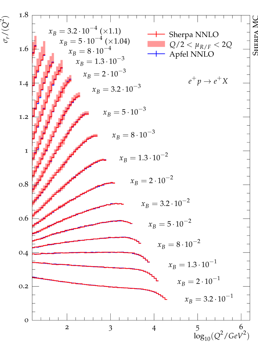
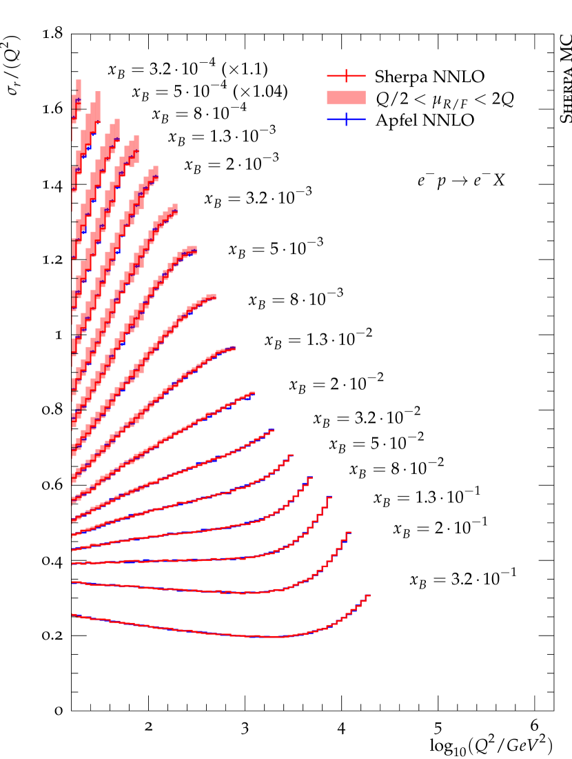
In order to validate our implementation of the Born differential NNLO cross section, we compare fixed-order predictions for the reduced cross section to results obtained with the publicly available A PFEL library Bertone (2018). The reduced cross section is defined as

$$\sigma_{r}=\frac{{\operatorname{d\!}\,}^{2}\sigma}{\operatorname{d\!}x\operatorname{d\!}Q^{2}}\frac{Q^{4}x}{2\pi\alpha^{2}Y_{+}}\;,$$ (13)

where $Y_{+}=(1+(1-y)^{2})$ and $y=Q^{2}/(sx)$ with $s$ the center-of-mass energy of the collider. As shown in Figure 2, where we show a comparison differentially in $Q^{2}$ and $x$, we observe good agreement within the statistical uncertainties. Note that for this cross-check we set the renormalization and factorization scale to $\mu_{R/F}^{2}=Q^{2}$.

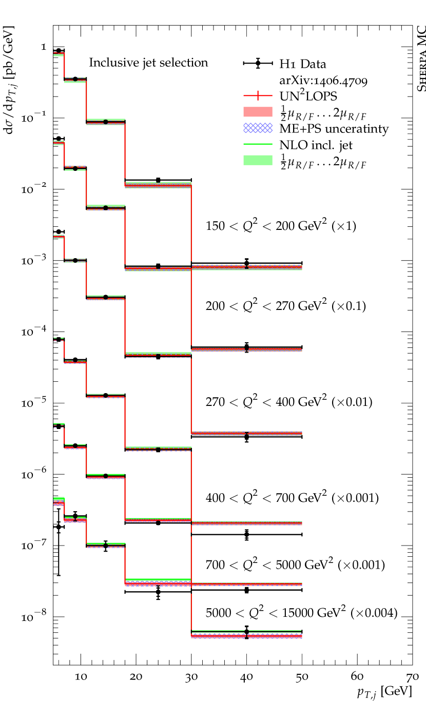
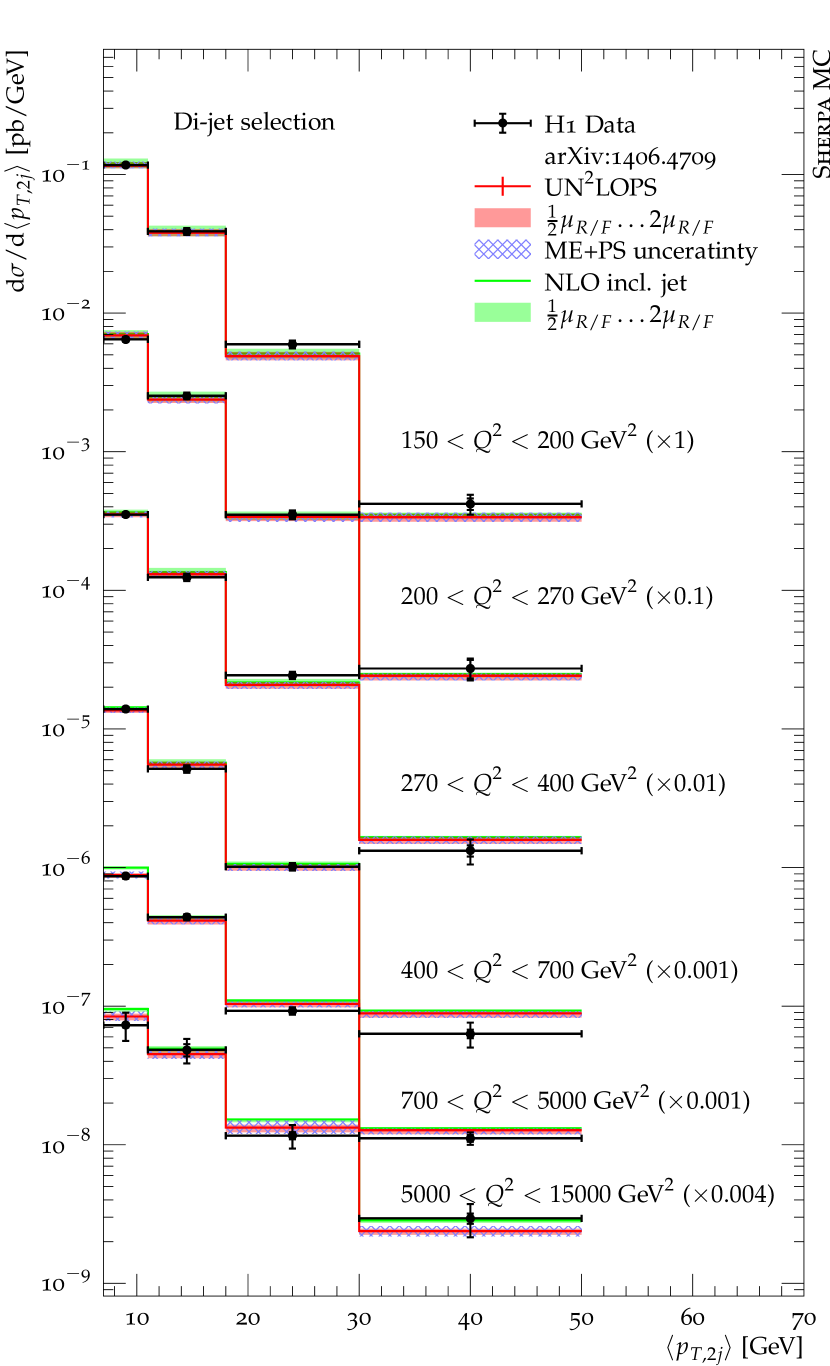
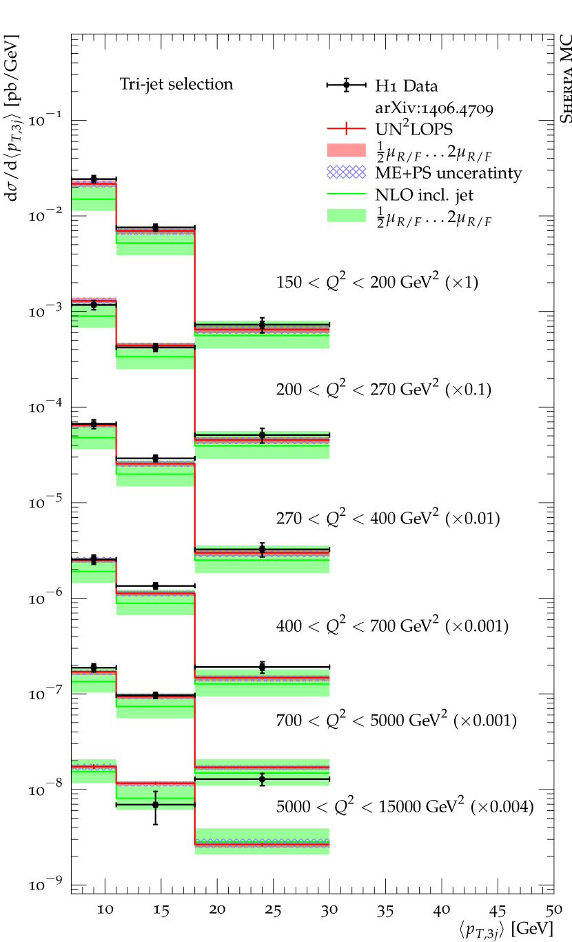
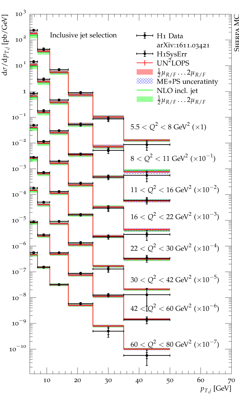
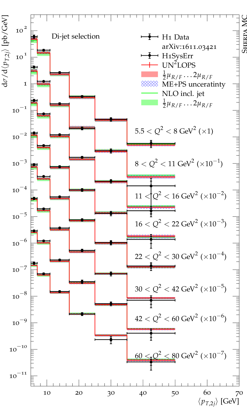
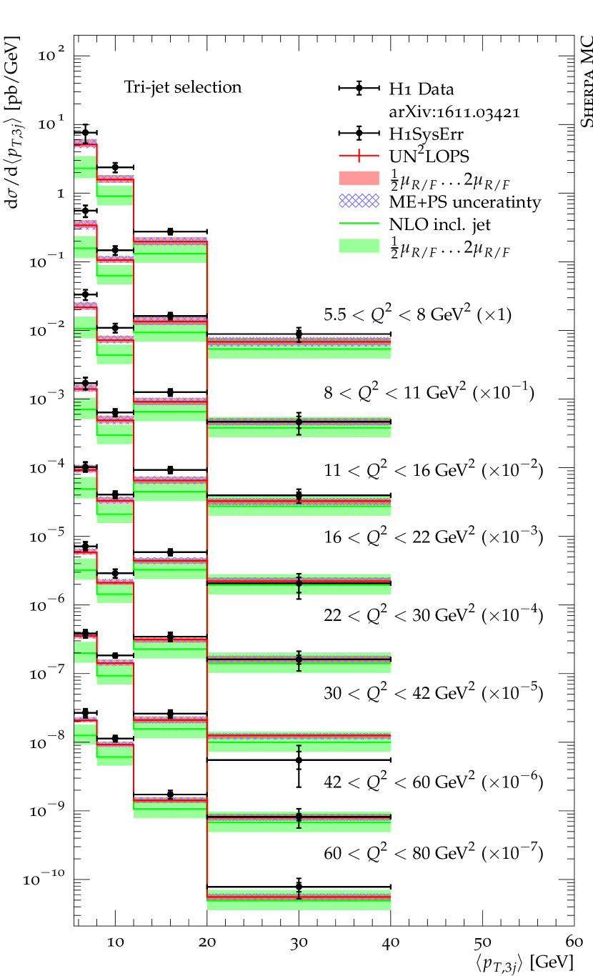
Figures 3 and 4 show the inclusive jet cross section, the di-jet cross section and the tri-jet cross section in the high and low $Q^{2}$ region as predicted by our simulations in comparison to experimental data from Andreev et al. (2015, 2017). The shaded uncertainty bands display the estimated theoretical uncertainties at fixed order and are obtained from a correlated variation of the renormalization and factorization scale by factors of two up and down. The hatched uncertainty band is a combination of the fixed-order uncertainties and the estimated parton-shower uncertainty, which is obtained by varying the scales at which the strong coupling and the PDF are evaluated in the parton shower by factors of $\sqrt{2}$ up and down, using the technique in Andersen et al. (2018). The parton-shower starting scale $\mu_{Q}$ is set to $Q^{2}$. Variations of this scale have a minor effect on our predictions, because the dominant hierarchy in the measurement phase space is such that $p_{T}>Q$. The predictions shown in green are obtained from a fixed-order NLO calculation for inclusive jet production. They have the same fixed-order accuracy as our parton shower matched simulations because the Born configurations of inclusive DIS do not contribute to the observables at fixed order. In the fixed-order predictions, we account for hadronization effects using the correction factors tabulated in Andreev et al. (2015, 2017). They are obtained in the usual fashion, i.e. by comparing leading-order parton shower Monte Carlo simulations before and after hadronization. The corresponding ratios are typically applied as multiplicative corrections to fixed-order calculations at the level of the observables. The predictions shown in red are obtained using our U NLOPS matched calculation supplemented with the string hadronization model Andersson et al. (1983); Andersson (1997). We observe good agreement between the matched calculation and the fixed-order prediction, which indicates that the QCD evolution and hadronization effects are well under control. Our results test and confirm, for the first time at this level of theoretical precision, the validity of the approach outlined above, where hadronization corrections are extracted from parton shower Monte Carlo simulations and then multiplicatively applied to the fixed-order calculation.

We quantify the size and uncertainty of the hadronization corrections in our simulations in Fig. 5. We plot the ratio between the particle-level predictions, with hadronization and hadron decays applied, to the prediction obtained after parton showering. We show two different results, one obtained using the Lund string fragmentation model Andersson et al. (1983); Andersson (1997) as implemented in P YTHIA  6.4 Sjöstrand et al. (2006) and one obtained using the cluster fragmentation model Field and Wolfram (1983); Webber (1984) as implemented in S HERPA  Winter et al. (2004). The perturbative input to the two simulations is identical, hence we quote their difference as the estimated hadronization uncertainty. We note that the hadronization corrections in our approach agree well with the results computed by H1, which are based on computations using D JANGOH  Charchula et al. (1994) and R AP G AP  Jung (1995). These two generators both include the exact expressions for the QCD Compton process at leading order, but D JANGOH uses the Lund dipole cascade model of A RIADNE  Lönnblad (1992) to simulate higher-order radiative corrections, while R AP G AP is based on collinear parton evolution. Both make use of the Lund string fragmentation model. It is encouraging that in our approach, using both a higher-order perturbative input and a different parton-shower model, the size of the hadronization corrections is very similar. In addition, the hadronization uncertainties are small, except for the very low transverse momentum region in the tri-jet cross section.

Figure 2: Comparison of NNLO cross sections, differential in $x$ and $Q^{2}$, between our dedicated implementation in S

HERPA

and the publicly available A

PFEL

library Bertone (2018).

Figure 3: Inclusive jet, di-jet and tri-jet cross section differential in $Q^{2}$ as a function of $p_{T,j}$ compared to experimental data from the H1 collaboration Andreev et al. (2015). We show separate error bars for the reported statistical and systematic uncertainties. We compare NLO fixed-order predictions corrected for hadronization effects (green) and parton-shower matched NNLO predictions at the particle level (red). The light green and light red uncertainty bands are obtained from a correlated variation of the renormalization and factorization scales. The hatched blue uncertainty band combines the fixed-order uncertainties and parton-shower uncertainties in quadrature. See the main text for details.

Figure 4: Inclusive jet cross section differential in $Q^{2}$ as a function of $p_{T,j}$ compared to experimental data from the H1 collaboration Andreev et al. (2017). See Fig. 3 and the main text for details.

Figure 5: Hadronization corrections determined using the U

NLOPS

simulation of DIS. Predictions from the Lund string model (red) are compared to results from the cluster fragmentation as implemented in S

HERPA

(blue) and to results computed by the H1 collaboration Andreev et al. (2015, 2017).

IV Conclusions

We have presented the first parton-shower matched calculation of hadronic final state production in DIS at NNLO QCD precision. The techniques needed to perform the simulation are implemented in the publicly available program S HERPA and can be used for event generation at the particle level. In contrast to earlier calculations using non-unitary multi-jet merging techniques, we are able to predict both jet production rates and inclusive quantities like structure functions within a single calculation. The agreement with recent analyses by the H1 collaboration is good. Since our calculation is based on collinear factorization, it can provide the basis for the reliable extraction of hadronization corrections needed in the comparison to fixed-order calculations.