Leabra7: a Python package for modeling recurrent, biologically-realistic neural networks

Abstract

Emergent (Aisa ., 2008) is a software package that uses the AdEx neural dynamics model (Brette  Gerstner, 2005) and LEABRA learning algorithm (O’Reilly, 1996) to simulate and train arbitrary recurrent neural network architectures in a biologically-realistic manner. We present Leabra7 (Greenidge  Miller, 2018), a complementary Python library that implements these same algorithms. Leabra7 is developed and distributed using modern software development principles, and integrates tightly with Python’s scientific stack. We demonstrate recurrent Leabra7 networks using traditional pattern-association tasks and a standard machine learning task, classifying the IRIS dataset.

1 Introduction

Advances in both cognitive modeling and machine learning research will depend on the ability to simulate and train recurrent neural networks. Nearly all brain areas contain recurrent circuitry (Shu ., 2003), from the visual system (Felleman  Van Essen, 1991) to the hypothesized canonical cortical microcircuit that grounds higher-order brain function (Douglas  Martin, 2007). Biologically plausible cognitive models must be able to simulate and train similarly recurrent architectures.

Deep learning is likewise dependent on recurrence. Recurrent neural networks commonly break records in sequence learning problems such as language translation (Schmidhuber, 2015). However, virtually all of these networks must use a specialized LSTM architecture to circumvent backpropagation’s vanishing gradient problem. A neural network model and learning algorithm that could handle arbitrary feedback connections would be able to take advantage of increasingly brain-like architectures, improving performance and computational efficiency (Schmidhuber, 2015).

Emergent (Aisa ., 2008) is a cognitive modeling framework designed to simulate and train these recurrent architectures. It does this by combining a biologically-plausible “adaptive-exponential” (AdEx) neural dynamics model (Brette  Gerstner, 2005) with LEABRA, a local, error-driven, biologically-realistic learning algorithm (O’Reilly, 1996). It has been used extensively by researchers to model the hippocampus (Schapiro ., 2017), prefrontal cortex and basal ganglia (Hazy ., 2007), and visual cortex (O’Reilly ., 2013), among other areas. In each case, the AdEx and LEABRA algorithms replicate important features of observed neural activity.

Leabra7 (Greenidge  Miller, 2018) is a new Python package that implements Emergent’s AdEx neural dynamics model and LEABRA learning algorithm. It allows researchers to quickly specify complex cognitive models using the full expressiveness of the Python programming language. Additionally, since Leabra7 is fully open-source and contains no compiled code, researchers can easily explore modifications to the LEABRA algorithm without a detailed knowledge of programming systems.

Leabra7 is developed and distributed with modern software engineering practices. It uses an event-driven architecture for low coupling, extensibility, and, in the future, parallel processing. Continuous integration, static analysis, and test-driven development ensure code quality. Both Leabra7 and its dependencies are continuously built and deployed to Anaconda Cloud, so users can install development and stable versions of Leabra7 via the conda package manager on Linux, MacOS, and Windows.

Finally, Leabra7 is deeply integrated with the scientific Python ecosystem. It natively operates on numpy arrays and pandas dataframes, and outputs data in a tidy format (Wickham, 2014), allowing downstream analysis using statistical best practices. Since it is distributed with conda, it is easy to leverage technologies for reproducible research, such as containers and Jupyter notebooks.

2 A brief tour of Leabra7’s API

2.1 Networks, layers, and projections

The Net (network) object is the primary component of any Leabra7 simulation: it manages every other object in the network and the interactions between them. Each simulation begins with the creation of the Net object and the addition of a few layers:

⬇

import leabra7 as lb

\parnet = lb.Net()

net.new_layer(name="input", size=3)

net.new_layer(name="output", size=3)

Here, the network has two layers, each containing three units, which are roughly equivalent to neurons.

Connections between layers are managed using Projn (projection) objects, which are simply bundles of unit-to-unit connections. Projections can have different connectivity patterns, but the most common is the “full” projection, where every unit in the sending layer connects to every unit in the receiving layer. Adding a projection between the input and output layers is accomplished with:

⬇

net.new_projn(name="input_to_output",

pre="input",

post="output")

Layers are referred to by their names, so that users do not have to touch the internal representation.

Once the network is constructed, time can be advanced using any of the following three methods:

⬇

net.cycle()

net.minus_phase_cycle(num_cycles=50)

net.plus_phase_cycle(num_cycles=25)

The first method simply steps the network forward in time. The last two methods run a series of cycles after triggering the minus or plus phases necessary for the LEABRA learning algorithm (see O’Reilly . (2012), for more information).

Finally, to compute and apply the weight changes using the LEABRA, the following method must be called:

⬇

net.learn()

2.2 Spec objects

The AdEx neural dynamics model and LEABRA learning algorithm contain many parameters. Like Emergent, Leabra7 manages parameters through Spec (specification) objects, which are simple record classes. Reasonable default parameters are provided automatically, but can be overridden by providing a custom Spec object during network creation. For example, to change a layer’s inhibition from the default feedforward/feedback to k-winner-take-all, the following code can be used:

⬇

import leabra7 as lb

\parnet = lb.Net()

net.new_layer(name="input",

size=3,

spec=lb.LayerSpec(inhibition_type="kwta"))

As much as possible, Leabra7 retains the names given to parameters in the Emergent software.

2.3 Output

Leabra7 outputs data in two forms: observations, which are instantaneous snapshots of the network state, and logs, which are series of observations recorded over time.

Observations are requested using the Net.observe() method. For example, the following code observes the output layer activation:

⬇

>> net.observe(name="output", attr="unit_act")

unit act

0 0 0.0

1 1 0.0

2 2 0.0

Here, the name parameter is the name of the object to observe, the attr parameter is the object attribute to observe, and the output is a Pandas dataframe. Observations can be requested for any attribute, on any object, at any time.

On the other hand, logging over time must be requested at network instantiation, through a Spec opbject. Here is an example of logging the output layer’s unit activation every cycle:

⬇

layer_spec = lb.LayerSpec(

log_on_cycle=("unit_act", )

)

net.new_layer(name="output", size=3, spec=layer_spec)

After a few cycles, the logs can be requested:

⬇

>> logs = net.logs(freq="cycle", name="output")

Because the activation is an attribute of the parts of the output layer, not of the entire layer itself (like the average activation), we access the parts member of the returned tuple:

⬇

>> logs.parts

unit act time

6 0 1.022608e-20 1

7 1 1.022608e-20 1

8 2 1.022608e-20 1

9 0 1.181225e-20 2

10 1 1.181225e-20 2

11 2 1.181225e-20 2

As before, the logs are stored in a Pandas dataframe, except that here the time column denotes the cycle at which the activation was recorded.

Since logging slows down network cycling and takes a considerable amount of memory, it is typically disabled during training and re-enabled only when needed, using the Net.pause_logging() and Net.resume_logging() methods.

3 Example networks

3.1 Two neurons

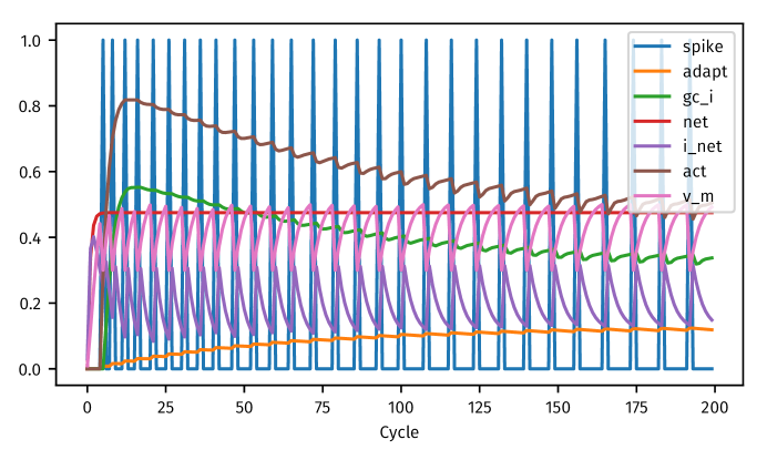
Figure 1: The internal dynamics of a spiking unit. See §3.1 for a detailed explanation of each quantity.

In the most basic network architecture, a single input unit is connected to a single output unit, with a connection weight of $0.5$. The input unit’s activation is clamped at a high value of $0.95$, so that it excites repeated spiking in the the output unit.

The dynamics of the output unit are shown in Figure 1. As the time-integrated excitatory input net rises, so does the net current into the unit, i_net. This drives the unit’s electric potential, v_m, above the spiking threshold, causing repeated spiking. When the unit spikes, the rate-coded activation value act increases, which would then be transmited to downstream, postsynaptic neurons if any existed. The spiking triggers feedback inhibition, gc_i, from the layer. Over time, the unit’s adaption current adapt increases, representing the onset of a refractory period, and spiking slows. When spiking slows, the activation act and inhibition gc_i drop.

3.2 Pattern association

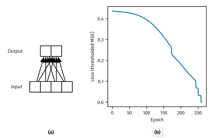
Figure 2: (a) The architecture of the pattern association network. Arrows represent connections between units. A size-2 input layer is connected to a size-4 output layer with a fully-connected projection. There is no hidden layer. (b) The thresholded mean-squared-error (MSE) loss during training, over 500 epochs. Thresholded MSE is similar to standard MSE, but errors less 0.5 are set to 0 (so the output activation only has to be on the correct side of 0.5). Because this is a strictly feedforward network, the loss curve decreases roughly monotonically.

A simple input-output architecture with no hidden layer (see Figure 2a) can be trained to recognize the following patterns, in which active units are dark:

To train the network, the input pattern is clamped to the network’s input layer, i.e. the input layer’s activations are set manually to the input pattern. The network is then cycled 50 to 75 times, to generate an output response. This is known as the “minus” phase. Then, in the “plus” phase, the correct output pattern is clamped to the output layer for an additional 20 to 25 cycles. Following the plus phase, the LEABRA algorithm is used to compute and apply weight changes that will reduce the error between the minus and plus phases. This procedure is repeated for each pattern in the training set, forming an epoch. The network loss over 500 training epochs is shown in Figure 2b.

3.3 Error-driven hidden

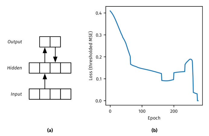
Figure 3: (a) The architecture of the error-driven hidden network. Arrows represent “projections”, which are groups of connections (in this case, connections which go from every unit in the sending layer to every unit in the receiving layer.) A recurrent feedback projection runs between the output and hidden layers to provide an error signal. (b) The thresholded sum-of-squared-error loss during training. The feedback connections induce high sensitivity to even tiny weight changes, causing oscillations in the loss curve. Such oscillations are not observed with feedforward architectures—see Figure 2.

The following patterns are an example of a nonlinear discrimination problem that cannot be learned using the simple pattern association architecture (O’Reilly  Rudy, 2000):

Intuitively, the simple architecture cannot learn the patterns because each input unit is active an equal amount for each output pattern. Mathematically, it is because the data are not linearly separable in $\mathbb{R}^{4}$. Introducing a hidden layer allows the network to solve such problems (Figure 3). A feedback connection is also required to provide an error response to the hidden layer during the plus phase of learning.

3.4 Classifying the IRIS dataset

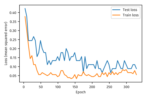
Figure 4: Training and test loss (mean squared error) for an input-hidden-output IRIS classifier. Network output was binarized by setting the largest value to 1 and all other values to 0. After 330 epochs, training classification accuracy was 95.83% and test classification accuracy was 90.00%.

The IRIS dataset is a standard machine learning classification benchmark (Fisher, 1936) containing 150 examples. The data consist of four input features: sepal length, sepal width, petal length, and petal width. The output class is one of three iris flower species: setosa, versicolor, or virginica.

We encoded the continuous input variables as follows: first, for each input value $x\in\mathbb{R}$, we estimated its quantile $q(x)$, which maps $x$ into the interval $[0,1]$. Next, we broke the $[0,1]$ interval into $n$ bins and recorded the index $i$ of the bin into which $q(x)$ falls. Finally, we encoded $i$ using a one-hot encoding, producing a vector with each value in $\{0,1\}$.

After preprocessing the data, we classified IRIS using the same input-hidden-output architecture described in Fig 3. Using $n=10$ bins, an input layer size of 36, and a hidden layer size of 23 produced satisfactory results. After 500 epochs of training on 80% of the dataset, we obtained a training accuracy of 95.83%, with a test accuracy of 90.00% on the remaining 20% (Figure 4).

4 Conclusion and future work

Leabra7 is a Pythonic, modern implementation of the LEABRA algorithm first implemented in Emergent (Aisa ., 2008). It is easy to modify, and integrates seamlessly into modern scientific workflows. We have shown that Leabra7 networks can learn both traditional pattern association tasks and standard machine learning tasks using feedforward and recurrent architectures as appropriate.

Before Leabra7 can be used to implement large cognitive models, like the hippocampal model described in Schapiro . (2017), performance must be improved in at least two areas. The first is learning performance: adaptive learning rate adjustment and annealing would greatly minimize late-stage loss oscillations. Second, a compiled engine in a language such as C++ would improve training speed for large networks, at the cost of making the algorithm more difficult to modify.

Appendix A Algorithm pseudocode

This section documents the exact algorithm that Leabra7 implements, as of v0.1.0. For a detailed explanation of the algorithm, see O’Reilly . (2012), and for default parameter values, see the file leabra7/specs.py in Leabra7’s source code. Nonessential features such as relative input scaling and Hebbian threshold modulation are omitted.

A.1 Network cycling

In a network cycle, the differential equations that govern the network dynamics are integrated forwards one step in time. This process consists of two stages. First, in the activation cycle, each unit is advanced one step forward in time. Typically, this causes the units to change their activation value. Then, in the projection flush, sending units propagate their new activations to receiving units.

1. Activation cycle

   For each layer, perform the following steps:

   1. For each unit, update net input.

      unit.net += integ * net_dt * (sum(inputs) - unit.net)
      

      unit.net is the unit’s net input, inputs is an array of activations sent to this unit in the projection flushing stage, integ is the global integration time constant, and net_dt is the net input integration time constant.

   2. Update layer-wide inhibition. These values are calculated at the layer level, but they are needed at the unit level for updating the membrane potential.

      Feedforward inhibition (ffi):

      ffi = ff * max(layer.avg_net - ff0, 0)
      

      ff is the feedforward inhibition multiplier, which controls the strength of feedforward inhibition, ff0 is the feedforward inhibition offset, and layer.avg_net is the average net input across the layer.

      Feedback inhibition (fbi):

      layer.fbi += fb_dt * (fb * net.avg_act - layer.fbi)
      

      fb is the feedback inhibition multiplier, which controls the strength of feedback inhibition, and fb_dt is the feedback inhibition integration time constant.

      Global inhibition (gc_i):

      layer.gc_i = gi * (ffi * layer.fbi)
      

      gi is the global inhibition multiplier, which controls overall inhibition strength.

   3. For each unit, update the net current i_net and membrane potential v_m.

      We maintain two versions of the net current and membrane potential: rate-coded, which approximates the discrete spiking rate with a number in the interval $[0,1]$, and non-rate-coded. The rate-coded version does not reset after each spike, and the non-rate-coded version does reset.

      First, calculate the non-rate-coded net current and membrane potential:

      unit.i_net = (unit.net * (e_rev_e - unit.v_m) +
                    gc_l * (e_rev_l - unit.v_m) +
                    layer.gc_i * (e_rev_i - unit.v_m))
      unit.v_m += clamp(integ * vm_dt * unit.i_net,
                        min=-100, max=100)
      

      We limit changes in v_m to be in the range $[-100,100]$ to avoid numerical integration problems. Here, e_rev_e is the excitatory reversal potential, e_rev_l is the leak reversal potential, and e_rev_i is the inhibitory reversal potential. gc_l is the leak conductance, which always remains constant.

      Next, calculate the rate-coded membrane potential, which does not reset when the unit spikes:

      unit.v_m_eq += clamp(integ * vm_dt * unit.i_net,
                           min=-100, max=100)
      

      The eq suffix denotes “equilibrium”.

   4. Update activation.

      Calculate the excitatory conductance (net input) that would place the unit at the spike threshold spk_thr:

      g_e_thr = (layer.gc_i * (e_rev_i - spk_thr) +
                 gc_l * (e_rev_l - spk_thr) -
                 unit.adapt) / (spk_thr - e_rev_e)
      

      adapt is the unit’s adaption current, which increases slowly as the unit activates and depresses the spike rate.

      Next, we handle discrete spiking. Discrete spiking is always calculated even with rate-coded activation, since adaption current depends on it.

      if unit.v_m > spk_thr:
          unit.v_m = v_m_r
          unit.spike = 1
      else:
          unit.spike = 0
      

      v_m_r is the reset value for the membrane potential after a spike.

      The unit activation can now be calculated and integrated forward in time:

      if unit.v_m_eq < unit.spk_thr:
          new_act = nxx1(unit.v_m_eq - spk_thr)
      else:
          new_act = nxx1(unit.net - g_e_thr)
      unit.act += integ * vm_dt * (new_act - unit.act)
      

      Before the first “spike”, the activation is governed by the v_m_eq dynamics, but after the first spike, it is driven by the g_e_thr term. nxx1 is the noisy $X/(X+1)$ activation function described in O’Reilly . (2012).

      Finally, the adaption current is calculated:

      unit.adapt += integ * adapt_dt * vm_gain * (vm_gain * (
          unit.v_m - e_rev_l)) + lunit.spike * spike_gain
      

      As usual, adapt_dt is the adaption current integration time constant. The constant vm_gain controls how much the membrane potential increases adaption current, and the constant spike_gain controls how much discrete spikes increase the adaption current.

   5. Update cycle learning averages.

      The LEABRA algorithm drives learning off of cascading activation averages: In general, the short-term averages encode the expected, or “plus-phase” value, while the medium-term average encodes the network’s current response, or “minus-phase” value mixed with the plus-phase value.

      The supershort, short, and medium-term learning averages that drive error-based learning are calculated every cycle:

      unit.avg_ss += integ * ss_dt * (
          unit.act - unit.avg_ss)
      unit.avg_s += integ * s_dt * (
          unit.avg_ss - unit.avg_s)
      unit.avg_m += integ * m_dt * (
          unit.avg_s - unit.avg_m)
      

      ss_dt, s_dt, and m_dt are the respective integration time constants.

      Every trial, the long-term learning average, which drives Hebbian learning, is calculated:

      if unit.avg_m > 0.1:
          unit.avg_l += unit.avg_m * l_up_inc
      else:
          unit.avg_l += acts_p_avg * l_dn_dt * (
              unit.avg_m - unit.avg_l)
      

      Note that the derivative of avg_l is bounded above $0.1$. l_dn_dt is the “downwards” integration time constant, and acts_p_avg is the average plus-phase activation across the layer.

2. Projection flushing.

   Once each unit’s activation has been updated, for each connection in each projection, we propagate the sending unit’s activation to the receiving unit, scaled by the connection weight:

   for connection in projection.connections:
       connection.receiving_unit.add_input(
           connection.weight * connection.sending_unit.act
       )
   

   The add_input function simply keeps the running sum of every added input, which is later integrated in the “update net input” step.

A.2 Learning

Learning trials consist of a “minus phase” of 50–75 cycles, followed by “plus phase” of 20–25 cycles. In the minus phase, the activations of the network’s input layers are set to the input pattern (also known as “clamping”), but the output layers are left untouched. In the plus phase, the input pattern is still clamped, and the desired output pattern is clamped on the network’s output layers.

In the following pseudocode, pre refers to the connection’s sending unit and post refers to the connection’s receiving unit.

After each trial, we compute the learning equations. First, the short- and medium-term learning coproducts, which encode the plus and minus-phase activations, respectively:

srs = post.avg_s * pre.avg_s
srm = post.avg_m * pre.avg_m
s_mix = 0.9
sm_mix = s_mix * srs + (1 - s_mix) * srm

Some of the medium-term coproduct is mixed into the short-term coproduct to drive weight depression if the receiving unit has $0$ activation in the plus phase.

Next, we calculate the long-term and medium-term floating thresholds, which encode Hebbian and error-driven learning, respectively:

lthr = post.avg_l * pre.avg_m * thr_l_mix
mthr = srm * (1 - thr_l_mix)

The constant thr_l_mix determines how much learning is Hebbian (based on lthr) and how much learning is error-driven (based on mthr).

Now we calculate the change (dwt) in the connection weight fwt:

dwt = lrate * xcal(sm_mix, lthr + mthr)
if dwt > 0:
    dwt *= 1 - fwt
else:
    dwt *= self.fwt
fwt += dwt

The multiplications ensure that the weight change slows down exponentially near $1$ and $0$.

Finally, we calculate wt, the sigmoidal contrast-enhanced weight used to propagate activation to the postsynaptic unit:

wt = 1 / (1 + (sig_offset * (1 - x) / x)^sig_gain)

The constant sig_offset controls the sigmoid translation and the constant sig_gain controls the sigmoid gain.

Appendix B Example network source code

B.1 Two neurons

⬇

import matplotlib.pyplot as plt

import pandas as pd #type: ignore

import leabra7 as lb

\par# Create the network

net = lb.Net()

\par# Log internal dynamics for each layer

layer_spec = lb.LayerSpec(

log_on_cycle=("unit_v_m", "unit_act", "unit_i_net", "unit_net",

"unit_gc_i", "unit_adapt", "unit_spike"))

\par# Instantiate the network

net.new_layer(name="input", size=1, spec=layer_spec)

net.new_layer(name="output", size=1, spec=layer_spec)

net.new_projn(name="proj1", pre="input", post="output")

\par# Activate the input layer

net.clamp_layer(name="input", acts=[1])

\par# Cycle the network

for i in range(200):

net.cycle()

\par# Retrieve logs

wholeLog, partLog = net.logs(freq="cycle", name="output")

\par# Plot the logs

ax = partLog.plot(x="time")

ax.set_xlabel("Cycle")

ax.legend(loc="upper right")

ax.figure.tight_layout()

ax.figure.savefig("two_neurons.png")

B.2 Pattern association

⬇

import logging

import sys

from typing import Dict

from typing import List

from typing import Iterable

from typing import Tuple

from typing import Union

\parimport numpy as np # type: ignore

import pandas as pd # type: ignore

\parimport leabra7 as lb # type: ignore

\parLoggerType = Union[None, logging.Logger, logging.LoggerAdapter]

\par\pardef load_data() -> Tuple[np.ndarray, np.ndarray]:

"""Loads and preprocesses the data.

\parReturns:

An (X, Y) tuple containing the features and labels, respectively.

\par"""

# yapf: disable

X = np.array([

[1, 1, 1, 0],

[0, 1, 1, 1],

[0, 1, 0, 1],

[0, 1, 0],

])

Y = np.array([

[1, 0],

[1, 0],

[0, 1],

[0, 1]

])

# yapf: enable

return (X, Y)

\par\pardef build_network(logger: LoggerType = None) -> lb.Net:

"""Builds the classifier network.

\parArgs:

logger: The logger to use.

\parReturns:

A Leabra7 network for classification.

\par"""

if logger is None:

logger = logging.getLogger()

logger.info("Building network")

net = lb.Net()

\par# Layers

layer_spec = lb.LayerSpec(

gi=1.5,

ff=1,

fb=0.5,

fb_dt=0.7,

log_on_epoch=("unit_act", ),

unit_spec=lb.UnitSpec(

adapt_dt=0,

vm_gain=0,

spike_gain=0,

ss_dt=1,

s_dt=0.2,

m_dt=0.15,

l_dn_dt=0.4,

l_up_inc=0.15,

vm_dt=0.3,

net_dt=0.7))

net.new_layer("input", size=4, spec=layer_spec)

net.new_layer("output", size=2, spec=layer_spec)

\par# Projections

spec = lb.ProjnSpec(

lrate=0.02,

dist=lb.Uniform(0.25, 0.75),

thr_l_mix=0.01,

cos_diff_lrate=False)

net.new_projn("input_to_output", pre="input", post="output", spec=spec)

\parreturn net

\par\pardef trial(network: lb.Net, input_pattern: Iterable[float],

output_pattern: Iterable[float]) -> None:

"""Runs a trial.

\parArgs:

input_pattern: The pattern to clamp to the network’s input layer.

output_pattern: The pattern to clamp to the network’s output layer.

\par"""

network.clamp_layer("input", input_pattern)

network.minus_phase_cycle(num_cycles=100)

network.clamp_layer("output", output_pattern)

network.plus_phase_cycle(num_cycles=20)

network.unclamp_layer("input")

network.unclamp_layer("output")

network.learn()

\par\pardef epoch(network: lb.Net, input_patterns: np.ndarray,

output_patterns: np.ndarray) -> None:

"""Runs an epoch (one pass through the whole dataset).

\parArgs:

input_patterns: A numpy array with shape (n_samples, n_features).

output_patterns: A numpy array with shape (n_samples, n_features).

\par"""

for x, y in zip(input_patterns, output_patterns):

trial(network, x, y)

network.end_epoch()

\par\pardef mse_thresh(expected: np.ndarray, actual: np.ndarray) -> float:

"""Calculates the thresholded mean squared error.

\parIf the error is < 0.5, it is treated as 0 (i.e., we count < 0.5 as 0 and

> 0.5 as 1).

\parArgs:

expected: The expected output pattern.

actual: The actual output pattern

\parReturns:

The thresholded mean squared error.

\par"""

diff = np.abs(expected - actual)

diff[diff < 0.5] = 0

return np.mean(diff * diff)

\par\pardef train(network: lb.Net,

input_patterns: np.ndarray,

output_patterns: np.ndarray,

num_epochs: int = 3000,

logger: LoggerType = None) -> pd.DataFrame:

"""Trains the network.

\parArgs:

input_patterns: A numpy array with shape (n_samples, n_features).

output_patterns: A numpy array with shape (n_samples, n_features).

num_patterns: The number of epochs to run. Defaults to 500.

logger: The logger to use. If None, will use the module’s default logger.

\parReturns:

pd.DataFrame: A dataframe of metrics from the training run.

\par"""

if logger is None:

logger = logging.getLogger()

logger.info("Begin training")

\pardata: Dict[str, List[float]] = {

"epoch": [],

"train_loss": [],

}

\parperfect_epochs = 0

for i in range(num_epochs):

epoch(network, input_patterns, output_patterns)

pred = predict(network, input_patterns)

data["epoch"].append(i)

data["train_loss"].append(mse_thresh(output_patterns, pred))

\parlogger.info("Epoch data["train_loss"][-1])

\parif data["train_loss"][-1] == 0:

perfect_epochs += 1

else:

perfect_epochs = 0

\parif perfect_epochs == 3:

logger.info("Ending training after perfect_epochs)

break

\parreturn pd.DataFrame(data)

\par\pardef output(network: lb.Net, pattern: Iterable[float]) -> List[float]:

"""Calculates a prediction for a single input pattern.

\parArgs:

network: The trained network.

pattern: The input pattern.

\parReturns:

np.ndarray: The output of the network after clamping the input

pattern to the input layer and settling. The max value is set to one,

everything else is set to zero.

\par"""

network.clamp_layer("input", pattern)

for _ in range(50):

network.cycle()

network.unclamp_layer("input")

out = network.observe("output", "unit_act")["act"].values

return list(out)

\par\pardef predict(network: lb.Net, input_patterns: np.ndarray) -> np.ndarray:

"""Calculates predictions for an array of input patterns.

\parArgs:

network (lb.Net): The trained network.

input_patterns (np.ndarray): An array of shape (n_samples, n_features)

containing the input patterns for which to calculate predictions.

\parReturns:

np.ndarray: An array of shape (n_samples, n_features) containing the

predictions for the input patterns.

\par"""

outputs = []

for item in input_patterns:

outputs.append(output(network, item))

return np.array(outputs)

\par\parif __name__ == "__main__":

PROJ_NAME = "pat_assoc"

\parlogging.basicConfig(

level=logging.DEBUG,

format="handlers=(logging.FileHandler(

"{0}_log.txt".format(PROJ_NAME), mode="w"),

logging.StreamHandler(sys.stdout)))

\parlogging.info("Begin training \parX, Y = load_data()

net = build_network()

metrics = train(net, X, Y)

\par# Save metrics and network for future analysis

metrics.to_csv("{0}_metrics.csv".format(PROJ_NAME), index=False)

net.save("{0}_network.pkl".format(PROJ_NAME))

B.3 Error-driven hidden

⬇

import logging

import sys

from typing import Dict

from typing import List

from typing import Iterable

from typing import Tuple

from typing import Union

\parimport numpy as np # type: ignore

import pandas as pd # type: ignore

\parimport leabra7 as lb # type: ignore

\parLoggerType = Union[None, logging.Logger, logging.LoggerAdapter]

\par\pardef load_data() -> Tuple[np.ndarray, np.ndarray]:

"""Loads and preprocesses the data.

\parReturns:

An (X, Y) tuple containing the features and labels, respectively.

\par"""

# yapf: disable

X = np.array([

[1, 0, 1, 0],

[0, 1, 0, 1],

[1, 1, 0, 0],

[0, 0, 1, 1,],

])

Y = np.array([

[1, 0],

[1, 0],

[0, 1],

[0, 1],

])

# yapf: enable

return (X, Y)

\par\pardef build_network(logger: LoggerType = None) -> lb.Net:

"""Builds the classifier network.

\parArgs:

logger: The logger to use.

\parReturns:

A Leabra7 network for classification.

\par"""

if logger is None:

logger = logging.getLogger()

logger.info("Building network")

net = lb.Net()

\par# Layers

layer_spec = lb.LayerSpec(

gi=1.5,

fb=1,

ff=1,

unit_spec=lb.UnitSpec(

adapt_dt=0,

vm_gain=0,

spike_gain=0,

ss_dt=1,

s_dt=0.2,

m_dt=0.1,

l_dn_dt=0.4,

l_up_inc=0.15,

vm_dt=1 / 3.3,

net_dt=0.7))

net.new_layer("input", size=4, spec=layer_spec)

net.new_layer("hidden", size=4, spec=layer_spec)

net.new_layer("output", size=2, spec=layer_spec)

\par# Projections

lrate = 0.04 # This is high, but it will be adaptively decreased

up_spec = lb.ProjnSpec(

lrate=lrate,

dist=lb.Uniform(0.25, 0.75),

thr_l_mix=0,

cos_diff_lrate=False,

cos_diff_thr_l_mix=True)

down_spec = lb.ProjnSpec(

lrate=lrate,

dist=lb.Uniform(0.25, 0.75),

wt_scale_rel=0.3,

thr_l_mix=0,

cos_diff_lrate=False,

cos_diff_thr_l_mix=True)

net.new_projn("input_to_hidden", pre="input", post="hidden", spec=up_spec)

net.new_projn(

"hidden_to_output", pre="hidden", post="output", spec=up_spec)

net.new_projn(

"output_to_hidden", pre="output", post="hidden", spec=down_spec)

\parreturn net

\par\pardef trial(network: lb.Net, input_pattern: Iterable[float],

output_pattern: Iterable[float]) -> None:

"""Runs a trial.

\parArgs:

input_pattern: The pattern to clamp to the network’s input layer.

output_pattern: The pattern to clamp to the network’s output layer.

\par"""

network.clamp_layer("input", input_pattern)

network.minus_phase_cycle(num_cycles=50)

network.clamp_layer("output", output_pattern)

network.plus_phase_cycle(num_cycles=20)

network.unclamp_layer("input")

network.unclamp_layer("output")

network.learn()

\par\pardef epoch(network: lb.Net, input_patterns: np.ndarray,

output_patterns: np.ndarray) -> None:

"""Runs an epoch (one pass through the whole dataset).

\parArgs:

input_patterns: A numpy array with shape (n_samples, n_features).

output_patterns: A numpy array with shape (n_samples, n_features).

\par"""

for x, y in zip(input_patterns, output_patterns):

trial(network, x, y)

network.end_epoch()

\par\pardef mse_thresh(expected: np.ndarray, actual: np.ndarray) -> float:

"""Calculates the thresholded mean squared error.

\parIf the error is < 0.5, it is treated as 0 (i.e., we count < 0.5 as 0 and

> 0.5 as 1).

\parArgs:

expected: The expected output pattern.

actual: The actual output pattern

\parReturns:

The thresholded mean squared error.

\par"""

diff = np.abs(expected - actual)

diff[diff < 0.5] = 0

return np.mean(diff * diff)

\par\pardef train(network: lb.Net,

input_patterns: np.ndarray,

output_patterns: np.ndarray,

num_epochs: int = 3000,

logger: LoggerType = None) -> pd.DataFrame:

"""Trains the network.

\parArgs:

input_patterns: A numpy array with shape (n_samples, n_features).

output_patterns: A numpy array with shape (n_samples, n_features).

num_patterns: The number of epochs to run. Defaults to 500.

logger: The logger to use. If None, will use the module’s default logger.

\parReturns:

pd.DataFrame: A dataframe of metrics from the training run.

\par"""

if logger is None:

logger = logging.getLogger()

logger.info("Begin training")

\pardata: Dict[str, List[float]] = {

"epoch": [],

"train_loss": [],

}

\parperfect_epochs = 0

for i in range(num_epochs):

epoch(network, input_patterns, output_patterns)

pred = predict(network, input_patterns)

data["epoch"].append(i)

data["train_loss"].append(mse_thresh(output_patterns, pred))

logger.info("Epoch data["train_loss"][-1])

\parif data["train_loss"][-1] == 0:

perfect_epochs += 1

else:

perfect_epochs = 0

\parif perfect_epochs == 3:

logger.info("Ending training after perfect_epochs)

break

\parreturn pd.DataFrame(data)

\par\pardef output(network: lb.Net, pattern: Iterable[float]) -> List[float]:

"""Calculates a prediction for a single input pattern.

\parArgs:

network: The trained network.

pattern: The input pattern.

\parReturns:

np.ndarray: The output of the network after clamping the input

pattern to the input layer and settling. The max value is set to one,

everything else is set to zero.

\par"""

network.clamp_layer("input", pattern)

for _ in range(50):

network.cycle()

network.unclamp_layer("input")

out = network.observe("output", "unit_act")["act"].values

return list(out)

\par\pardef predict(network: lb.Net, input_patterns: np.ndarray) -> np.ndarray:

"""Calculates predictions for an array of input patterns.

\parArgs:

network: The trained network.

input_patterns: An array of shape (n_samples, n_features)

containing the input patterns for which to calculate predictions.

\parReturns:

np.ndarray: An array of shape (n_samples, n_features) containing the

predictions for the input patterns.

\par"""

outputs = []

for item in input_patterns:

outputs.append(output(network, item))

return np.array(outputs)

\par\parif __name__ == "__main__":

PROJ_NAME = "err_hidden"

\parlogging.basicConfig(

level=logging.DEBUG,

format="handlers=(logging.FileHandler(

"{0}_log.txt".format(PROJ_NAME), mode="w"),

logging.StreamHandler(sys.stdout)))

\parlogging.info("Begin training \parX, Y = load_data()

net = build_network()

metrics = train(net, X, Y)

\par# Save metrics and network for future analysis

metrics.to_csv("{0}_metrics.csv".format(PROJ_NAME), index=False)

net.save("{0}_network.pkl".format(PROJ_NAME))

B.4 Classifying the IRIS dataset

⬇

import logging

import sys

from typing import Any

from typing import Dict

from typing import List

from typing import Iterable

from typing import Tuple

from typing import Union

\parimport numpy as np # type: ignore

import pandas as pd # type: ignore

import sklearn.datasets # type: ignore

import sklearn.metrics # type: ignore

import sklearn.model_selection # type: ignore

import sklearn.preprocessing # type: ignore

\parimport leabra7 as lb # type: ignore

\parLoggerType = Union[None, logging.Logger, logging.LoggerAdapter]

\par\pardef load_data(num_feature_units: int = 10,

logger: LoggerType = None) -> Tuple[np.ndarray, np.ndarray]:

"""Loads and preprocesses the data.

\parReturns:

An (X, Y) tuple containing the features and labels, respectively.

\par"""

if logger is None:

logger = logging.getLogger()

logger.info("Loading data")

data = sklearn.datasets.load_iris()

\par# One-hot encode the labels

label_binarizer = sklearn.preprocessing.LabelBinarizer()

Y = label_binarizer.fit_transform(data.target)

\par# Quantile transform, bin, and one-hot encode the features

quant = sklearn.preprocessing.QuantileTransformer()

X = quant.fit_transform(data.data)

X = np.digitize(X, bins=np.linspace(0.0, 1.0, num=num_feature_units))

one_hot = sklearn.preprocessing.OneHotEncoder(sparse=False)

X = one_hot.fit_transform(X)

\par# Randomly shuffle the data

return sklearn.utils.shuffle(X, Y)

\par\pardef build_network(input_size: int,

output_size: int,

hidden_size: int = 23,

logger: LoggerType = None) -> lb.Net:

"""Builds the classifier network.

\parArgs:

input_size: The size of the input layer.

output_size: The size of the output layer.

hidden_size: The size of the hidden layer.

logger: The logger to use.

\parReturns:

A Leabra7 network for classification.

\par"""

if logger is None:

logger = logging.getLogger()

logger.info("Building network")

net = lb.Net()

\par# Layers

layer_spec = lb.LayerSpec(gi=1.5, ff=1, fb=1,

unit_spec=lb.UnitSpec(spike_gain=0, vm_gain=0, adapt_dt=0))

net.new_layer("input", size=input_size, spec=layer_spec)

net.new_layer("hidden", size=hidden_size, spec=layer_spec)

net.new_layer("output", size=output_size, spec=layer_spec)

logger.debug("Input layer size: logger.debug("Hidden layer size: logger.debug("Output layer size: \par# Projections

lrate = 0.02

up_spec = lb.ProjnSpec(

lrate=lrate,

dist=lb.Uniform(0.25, 0.75),

cos_diff_thr_l_mix=False,

cos_diff_lrate=False)

down_spec = lb.ProjnSpec(

lrate=lrate,

dist=lb.Uniform(0.25, 0.5),

wt_scale_rel=0.3,

cos_diff_thr_l_mix=False,

cos_diff_lrate=False)

net.new_projn("input_to_hidden", pre="input", post="hidden", spec=up_spec)

net.new_projn(

"hidden_to_output", pre="hidden", post="output", spec=up_spec)

net.new_projn(

"output_to_hidden", pre="output", post="hidden", spec=down_spec)

\parreturn net

\par\pardef trial(network: lb.Net, input_pattern: Iterable[float],

output_pattern: Iterable[float]) -> None:

"""Runs a trial.

\parArgs:

input_pattern: The pattern to clamp to the network’s input layer.

output_pattern: The pattern to clamp to the network’s output layer.

\par"""

network.clamp_layer("input", input_pattern)

network.minus_phase_cycle(num_cycles=50)

network.clamp_layer("output", output_pattern)

network.plus_phase_cycle(num_cycles=25)

network.unclamp_layer("input")

network.unclamp_layer("output")

network.learn()

\par\pardef epoch(network: lb.Net, input_patterns: np.ndarray,

output_patterns: np.ndarray) -> None:

"""Runs an epoch (one pass through the whole dataset).

\parArgs:

input_patterns: A numpy array with shape (n_samples, n_features).

output_patterns: A numpy array with shape (n_samples, n_features).

\par"""

for x, y in zip(input_patterns, output_patterns):

trial(network, x, y)

network.end_epoch()

\par\pardef train(network: lb.Net,

input_patterns: np.ndarray,

output_patterns: np.ndarray,

num_epochs: int = 500,

logger: LoggerType = None) -> pd.DataFrame:

"""Trains the network.

\parArgs:

input_patterns: A numpy array with shape (n_samples, n_features).

output_patterns: A numpy array with shape (n_samples, n_features).

num_patterns: The number of epochs to run. Defaults to 500.

logger: The logger to use. If None, will use the module’s default logger.

\parReturns:

pd.DataFrame: A dataframe of metrics from the training run.

\par"""

if logger is None:

logger = logging.getLogger()

logger.info("Begin training")

\parX_train, X_test, Y_train, Y_test = sklearn.model_selection.train_test_split(

input_patterns, output_patterns, test_size=0.2)

\parlogger.debug("Training set size: logger.debug("Test set size: \pardata: Dict[str, List[float]] = {

"epoch": [],

"train_loss": [],

"train_accuracy": [],

"test_loss": [],

"test_accuracy": []

}

\parfor i in range(num_epochs):

epoch(network, X_train, Y_train)

\par# Predicting is slow, so we only calculate metrics every 5 epochs

if (i + 1) pred_train = predict(network, X_train)

data["epoch"].append(i)

data["train_loss"].append(

sklearn.metrics.mean_squared_error(Y_train, pred_train))

data["train_accuracy"].append(

sklearn.metrics.accuracy_score(

Y_train, pred_train, normalize=True))

\parpred_test = predict(network, X_test)

data["test_loss"].append(

sklearn.metrics.mean_squared_error(Y_test, pred_test))

data["test_accuracy"].append(

sklearn.metrics.accuracy_score(

Y_test, pred_test, normalize=True))

logger.info(

"Epoch i, num_epochs, data["train_accuracy"][-1] * 100,

data["test_accuracy"][-1] * 100)

\parlogger.info("End training")

return pd.DataFrame(data)

\par\pardef output(network: lb.Net, pattern: Iterable[float]) -> List[float]:

"""Calculates a prediction for a single input pattern.

\parArgs:

network: The trained network.

pattern: The input pattern.

\parReturns:

np.ndarray: The output of the network after clamping the input

pattern to the input layer and settling. The max value is set to one,

everything else is set to zero.

\par"""

network.clamp_layer("input", pattern)

for _ in range(50):

network.cycle()

network.unclamp_layer("input")

out = network.observe("output", "unit_act")["act"].values

max_idx = np.argmax(out)

out[:] = 0

out[max_idx] = 1

return list(out)

\par\pardef predict(network: lb.Net, input_patterns: np.ndarray) -> np.ndarray:

"""Calculates predictions for an array of input patterns.

\parArgs:

network: The trained network.

input_patterns: An array of shape (n_samples, n_features)

containing the input patterns for which to calculate predictions.

\parReturns:

np.ndarray: An array of shape (n_samples, n_features) containing the

predictions for the input patterns.

\par"""

outputs = []

for item in input_patterns:

outputs.append(output(network, item))

return np.array(outputs)

\par\parif __name__ == "__main__":

PROJ_NAME = "iris"

np.seterr("warn")

\parlogging.basicConfig(

level=logging.DEBUG,

format="handlers=(logging.FileHandler(

"{0}_log.txt".format(PROJ_NAME), mode="w"),

logging.StreamHandler(sys.stdout)))

\parlogging.info("Begin training \parX, Y = load_data()

net = build_network(input_size=X.shape[1], output_size=Y.shape[1])

metrics = train(net, X, Y)

\par# Save metrics and network for future analysis

metrics.to_csv("{0}_metrics.csv".format(PROJ_NAME), index=False)

net.save("{0}_network.pkl".format(PROJ_NAME))

References

- Aisa \BOthers. (\APACyear2008) \APACinsertmetastaraisaEmergentNeuralModeling2008{APACrefauthors}Aisa, B., Mingus, B.\BCBL \BBA O’Reilly, R. \APACrefYearMonthDay2008. \BBOQ\APACrefatitleThe Emergent Neural Modeling System The Emergent neural modeling system.\BBCQ \APACjournalVolNumPagesNeural Networks2181146-1152. {APACrefDOI} \doi10.1016/j.neunet.2008.06.016 \PrintBackRefs\CurrentBib
- Brette \BBA Gerstner (\APACyear2005) \APACinsertmetastarbretteAdaptiveExponentialIntegrateandFire2005{APACrefauthors}Brette, R.\BCBT \BBA Gerstner, W. \APACrefYearMonthDay2005. \BBOQ\APACrefatitleAdaptive Exponential Integrate-and-Fire Model as an Effective Description of Neuronal Activity Adaptive Exponential Integrate-and-Fire Model as an Effective Description of Neuronal Activity.\BBCQ \APACjournalVolNumPagesJournal of Neurophysiology9453637-3642. {APACrefDOI} \doi10.1152/jn.00686.2005 \PrintBackRefs\CurrentBib
- Douglas \BBA Martin (\APACyear2007) \APACinsertmetastardouglasMappingMatrixWays2007{APACrefauthors}Douglas, R\BPBIJ.\BCBT \BBA Martin, K\BPBIA\BPBIC. \APACrefYearMonthDay2007\APACmonth10. \BBOQ\APACrefatitleMapping the Matrix: The Ways of Neocortex Mapping the Matrix: The Ways of Neocortex.\BBCQ \APACjournalVolNumPagesNeuron562226-238. {APACrefDOI} \doi10.1016/j.neuron.2007.10.017 \PrintBackRefs\CurrentBib
- Felleman \BBA Van Essen (\APACyear1991) \APACinsertmetastarfellemanDistributedHierarchicalProcessing1991{APACrefauthors}Felleman, D\BPBIJ.\BCBT \BBA Van Essen, D\BPBIC. \APACrefYearMonthDay1991. \BBOQ\APACrefatitleDistributed Hierarchical Processing in the Primate Cerebral Cortex. Distributed hierarchical processing in the primate cerebral cortex.\BBCQ \APACjournalVolNumPagesCerebral cortex (New York, N.Y. : 1991)111-47. {APACrefDOI} \doi10.1093/cercor/1.1.1 \PrintBackRefs\CurrentBib
- Fisher (\APACyear1936) \APACinsertmetastarfisherUseMultipleMeasurements1936{APACrefauthors}Fisher, R\BPBIA. \APACrefYearMonthDay1936. \BBOQ\APACrefatitleThe Use of Multiple Measurements in Taxonomic Problems The Use of Multiple Measurements in Taxonomic Problems.\BBCQ \APACjournalVolNumPagesAnnals of Eugenics72179-188. {APACrefDOI} \doi10.1111/j.1469-1809.1936.tb02137.x \PrintBackRefs\CurrentBib
- Greenidge \BBA Miller (\APACyear2018) \APACinsertmetastargreenidgeCdgreenidgeLeabra7V02018{APACrefauthors}Greenidge, C\BPBID.\BCBT \BBA Miller, N. \APACrefYearMonthDay2018\APACmonth09. \BBOQ\APACrefatitleCdgreenidge/Leabra7: V0.1.0 Cdgreenidge/leabra7: V0.1.0.\BBCQ {APACrefDOI} \doi10.5281/zenodo.1411499 \PrintBackRefs\CurrentBib
- Hazy \BOthers. (\APACyear2007) \APACinsertmetastarhazyExecutiveHomunculusComputational2007{APACrefauthors}Hazy, T\BPBIE., Frank, M\BPBIJ.\BCBL \BBA O’Reilly, R\BPBIC. \APACrefYearMonthDay2007. \BBOQ\APACrefatitleTowards an Executive without a Homunculus: Computational Models of the Prefrontal Cortex/Basal Ganglia System Towards an executive without a homunculus: Computational models of the prefrontal cortex/basal ganglia system.\BBCQ \APACjournalVolNumPagesPhilosophical Transactions of the Royal Society of London B: Biological Sciences36214851601-1613. {APACrefDOI} \doi10.1098/rstb.2007.2055 \PrintBackRefs\CurrentBib
- O’Reilly (\APACyear1996) \APACinsertmetastaroreillyLEABRAModelNeural1996{APACrefauthors}O’Reilly, R\BPBIC. \APACrefYearMonthDay1996. \BBOQ\APACrefatitleThe LEABRA Model of Neural Interactions and Learning in the Neocortex The LEABRA model of neural interactions and learning in the neocortex.\BBCQ \APACjournalVolNumPagesProQuest Dissertations and Theses. \PrintBackRefs\CurrentBib
- O’Reilly \BOthers. (\APACyear2012) \APACinsertmetastaroreillyComputationalCognitiveNeuroscience2012{APACrefauthors}O’Reilly, R\BPBIC., Munakata, Y., Frank, M\BPBIJ., Hazy, T\BPBIE.\BCBL \BBA Contributors. \APACrefYear2012. \APACrefbtitleComputational Cognitive Neuroscience Computational Cognitive Neuroscience (\PrintOrdinal1 \BEd). \APACaddressPublisherWiki Book. \PrintBackRefs\CurrentBib
- O’Reilly \BBA Rudy (\APACyear2000) \APACinsertmetastaroreillyComputationalPrinciplesLearning2000{APACrefauthors}O’Reilly, R\BPBIC.\BCBT \BBA Rudy, J\BPBIW. \APACrefYearMonthDay2000. \BBOQ\APACrefatitleComputational Principles of Learning in the Neocortex and Hippocampus Computational principles of learning in the neocortex and hippocampus.\BBCQ \APACjournalVolNumPagesHippocampus104389-397. {APACrefDOI} \doi10.1002/1098-1063(2000)10:4<389::AID-HIPO5>3.0.CO;2-P \PrintBackRefs\CurrentBib
- O’Reilly \BOthers. (\APACyear2013) \APACinsertmetastaroreillyRecurrentProcessingObject2013{APACrefauthors}O’Reilly, R\BPBIC., Wyatte, D., Herd, S., Mingus, B.\BCBL \BBA Jilk, D\BPBIJ. \APACrefYearMonthDay2013. \BBOQ\APACrefatitleRecurrent Processing during Object Recognition Recurrent Processing during Object Recognition.\BBCQ \APACjournalVolNumPagesFrontiers in Psychology4. {APACrefDOI} \doi10.3389/fpsyg.2013.00124 \PrintBackRefs\CurrentBib
- Schapiro \BOthers. (\APACyear2017) \APACinsertmetastarschapiroComplementaryLearningSystems2017{APACrefauthors}Schapiro, A\BPBIC., Turk-Browne, N\BPBIB., Botvinick, M\BPBIM.\BCBL \BBA Norman, K\BPBIA. \APACrefYearMonthDay2017. \BBOQ\APACrefatitleComplementary Learning Systems within the Hippocampus: A Neural Network Modelling Approach to Reconciling Episodic Memory with Statistical Learning Complementary learning systems within the hippocampus: A neural network modelling approach to reconciling episodic memory with statistical learning.\BBCQ \APACjournalVolNumPagesPhil. Trans. R. Soc. B372171120160049. {APACrefDOI} \doi10.1098/rstb.2016.0049 \PrintBackRefs\CurrentBib
- Schmidhuber (\APACyear2015) \APACinsertmetastarschmidhuberDeepLearningNeural2015{APACrefauthors}Schmidhuber, J. \APACrefYearMonthDay2015. \BBOQ\APACrefatitleDeep Learning in Neural Networks: An Overview Deep Learning in Neural Networks: An Overview.\BBCQ \APACjournalVolNumPagesNeural Networks6185-117. {APACrefDOI} \doi10.1016/j.neunet.2014.09.003 \PrintBackRefs\CurrentBib
- Shu \BOthers. (\APACyear2003) \APACinsertmetastarshuTurningRecurrentBalanced2003{APACrefauthors}Shu, Y., Hasenstaub, A.\BCBL \BBA McCormick, D\BPBIA. \APACrefYearMonthDay2003. \BBOQ\APACrefatitleTurning on and off Recurrent Balanced Cortical Activity Turning on and off recurrent balanced cortical activity.\BBCQ \APACjournalVolNumPagesNature4236937288-293. {APACrefDOI} \doi10.1038/nature01616 \PrintBackRefs\CurrentBib
- Wickham (\APACyear2014) \APACinsertmetastarwickhamhadleyTidyData2014{APACrefauthors}Wickham, H. \APACrefYearMonthDay2014. \BBOQ\APACrefatitleTidy Data Tidy Data.\BBCQ \APACjournalVolNumPagesJournal of Statistical Software5910. {APACrefDOI} \doi10.18637/jss.v059.i10 \PrintBackRefs\CurrentBib