Abstract

We provide the first importance sampling variants of variance-reduced algorithms for empirical risk minimization with non-convex loss functions. In particular, we analyze non-convex versions of SVRG, SAGA and SARAH. Our methods have the capacity to speed up the training process by an order of magnitude compared to the state of the art on real datasets. Moreover, we also improve upon current mini-batch analysis of these methods by proposing importance sampling for minibatches in this setting. Ours are the first optimal samplings for minibatches in the literature on stochastic optimization. Surprisingly, our approach can in some regimes lead to superlinear speedup with respect to the minibatch size, which is not usually present in stochastic optimization. All the above results follow from a general analysis of the methods which works with arbitrary sampling, i.e., fully general randomized strategy for the selection of subsets of examples to be sampled in each iteration. Finally, we also perform a novel importance sampling analysis of SARAH in the convex setting.

1 Introduction

Empirical risk minimization (ERM) is a key problem in machine learning as it plays a key role in training supervised learning models, including classification and regression problems, such as support vector machine, logistic regression and deep learning. A generic ERM problem has the finite-sum form

$$\min_{x}\ f(x):=\frac{1}{n}\sum_{i=1}^{n}f_{i}(x),$$ (1)

where $x$ corresponds to the parameters defining a model, $f_{i}(x)$ is the loss of the model $x$ associated with data point $i$, and $f$ is the average (empirical) loss across the entire training dataset. In this paper we focus on the case when the functions $f_{i}$ are $L_{i}$–smooth but non-convex. We assume the problem has a solution $x^{*}$.

One of the most popular algorithms for solving (1) is stochastic gradient descent (SGD) (Nemirovsky and Yudin, 1983; Nemirovski et al., 2009). In recent years, tremendous effort was exerted to improve its performance, leading to various enhancements which use acceleration Allen-Zhu (2016), momentum Loizou and Richtárik (2017), minibatching Takáč et al. (2013), distributed implementation Ma et al. (2015; 2017), importance sampling Zhao and Zhang (2015); Csiba and Richtárik (2018); Qu et al. (2015); Chambolle et al. (2018), higher-order information Qu et al. (2016); Gower et al. (2016), and a number of other techniques.

1.1 Variance-reduced methods

A particularly important recent advance has to do with the design of variance-reduced (VR) stochastic gradient methods, such as SAG (Roux et al., 2012), SDCA (Shalev-Shwartz and Zhang, 2013; Richtárik and Takáč, 2014), SVRG (Johnson and Zhang, 2013), S2GD (Konečný and Richtárik, 2017), SAGA (Defazio et al., 2014a), MISO (Mairal, 2015), FINITO (Defazio et al., 2014b) and SARAH (Nguyen et al., 2017a), which operate by modifying the classical stochastic gradient direction in each step of the training process in various clever ways so as to progressively reduce its variance as an estimator of the true gradient. We note that SAG and SARAH, historically the oldest and one the newest VR methods in the list, respectively, use a biased estimator of the gradient. In theory, all these methods enjoy linear convergence rates on smooth and strongly convex functions, which is in contrast with slow sublinear rate of SGD. VR methods are also easier to implement as they do not rely on a decreasing learning rate schedule. VR methods were recently extended to work with (non-strongly) convex losses by Konečný and Richtárik (2017), and more recently also to non-convex losses by Reddi et al. (2016b; a); Allen-Zhu and Hazan (2016); Nguyen et al. (2017b) - in all cases leading to best current rates for (1) in a given function class.

1.2 Importance sampling, minibatching and non-convex models

In the context of problem (1), importance sampling refers to the technique of assigning carefully designed non-uniform probabilities $\{p_{i}\}$ to the $n$ functions $\{f_{i}\}$, and using these, as opposed to uniform probabilities, to sample the next data point (stochastic gradient) during the training process.

Despite the huge theoretical and practical success of VR methods, there are still considerable gaps in our understanding. For instance, an importance sampling variant of the popular SAGA method, with the “correct” convergence rate, was only designed very recently by Gower et al. (2018); and the analysis applies to strongly convex $f$ only. A coordinate descent variant of SVRG with importance sampling, also in the strongly convex case, was analyzed by Konečný et al. (2017). However, the method does not seem to admit a fast implementation. For dual methods based on coordinate descent, importance sampling is relatively well understood (Nesterov, 2012; Richtárik and Takáč, 2014; Qu and Richtárik, 2016; Qu et al., 2015; Allen-Zhu et al., 2016).

The territory is completely unmapped in the non-convex case, however. To the best of our knowledge, no importance sampling VR methods have been designed nor analyzed in the popular case when the functions $\{f_{i}\}$ are non-convex. An exception to this is dfSDCA (Csiba and Richtárik, 2015); however, this method applies to an explicitly regularized version of (1), and while the individual functions are allowed to be non-convex, the average $f$ is assumed to be convex. Given the dominance of stochastic gradient type methods in training large non-convex models such as deep neural networks, theoretical investigation of VR methods that can benefit from importance sampling is much needed.

The situation is worse still when one asks for importance sampling of minibatches. To the best of our knowledge, there are only a handful of papers on this topic (Richtárik and Takáč, 2016a; Csiba and Richtárik, 2018; Hanzely and Richtárik, 2019), none of which apply to the non-convex setting considered here, nor to the methods we will analyze, and the problem is open. This is despite the fact that minibatch methods are de-facto the norm for training deep nets. In practice, typically relatively small (${\cal O}(1)$ or ${\cal O}(\log n)$) minibatch sizes are used.

1.3 Contributions

Algorithm	Uniform sampling	Arbitrary sampling [NEW]	$S^{*}$ sampling [NEW]
SVRG	$\max\left\{n,\frac{{\color[rgb]{.75,0,.25}(1+\nicefrac{{4}}{{3}})L_{\max}}c_{1}n^{2/3}}{\epsilon}\right\}$	$\max\left\{n,\frac{{\color[rgb]{.75,0,.25}(1+\nicefrac{{4\alpha}}{{3}})\bar{L}}c_{1}n^{2/3}}{\epsilon}\right\}$	$\max\left\{n,\frac{{\color[rgb]{.75,0,.25}\left(1+\frac{4(n-b)}{3n}\right)\bar{L}}c_{1}n^{2/3}}{\epsilon}\right\}$
SAGA	$n+\frac{{\color[rgb]{.75,0,.25}2L_{\max}}c_{2}n^{2/3}}{\epsilon}$	$n+\frac{{\color[rgb]{.75,0,.25}(1+\alpha)\bar{L}}c_{2}n^{2/3}}{\epsilon}$	$n+\frac{{\color[rgb]{.75,0,.25}(1+\frac{n-b}{n})\bar{L}}c_{2}n^{2/3}}{\epsilon}$
SARAH	$n+\frac{{\color[rgb]{.75,0,.25}\frac{n-b}{n-1}L_{\max}^{2}}c_{3}}{\epsilon^{2}}$	$n+\frac{{\color[rgb]{.75,0,.25}\alpha\bar{L}^{2}}c_{3}}{\epsilon^{2}}$	$n+\frac{{\color[rgb]{.75,0,.25}\frac{n-b}{n}\bar{L}^{2}}c_{3}}{\epsilon^{2}}$

Table 1: Stochastic gradient evaluation complexity for achieving ${{\rm E}}\left[\|\nabla f(x)\|^{2}\right]\leq\epsilon$ for two variants of SVRG, SAGA and SARAH for minimizing the average of smooth non-convex functions. Constants: $c_{1},c_{2},c_{3}$ are universal constant, $L_{\max}=\max_{i}L_{i}$; $\bar{L}=\tfrac{1}{n}\sum_{i}L_{i}$; $b$ = (average) minibatch size (hidden in $\alpha$); $\alpha$ can be for specific samplings smaller than $1$ and decreasing with increasing $b$, which can lead to superlinear speedup in $b$. For SARAH this guarantee holds for one outer loop with minibatch size, where we assume $16\bar{L}^{2}(f(x^{0})-f(x^{*})^{2})/(\epsilon b)^{2}\gg 0$, in other words, minibatch size is not too big comparing to the required precision.

The main contributions of this paper are:

Arbitrary sampling. We peform a general analysis of three popular VR methods—SVRG (Johnson and Zhang, 2013), SAGA (Defazio et al., 2014a) and SARAH (Nguyen et al., 2017a)—in the arbitrary sampling paradigm (Richtárik and Takáč, 2016a; Qu and Richtárik, 2016; 2016; Qu et al., 2015; Chambolle et al., 2018). That is, we prove general complexity results which hold for an arbitrary random set valued mapping (aka arbitrary sampling) generating the minibatches of examples used by the algorithms in each iteration.

Optimal sampling. Starting from our general complexity results which hold for arbitrary sampling (see the second column in Table 1), we are able calculate the optimal sampling out of all samplings of a given minibatch size (see Lemma 2 and also the last column in Table 1). This is the first time an optimal minibatch sampling was computed (from the class of all samplings) in the literature for any stochastic optimization method we know, including all variants of SGD and coordinate descent. Indeed, while the results in (Richtárik and Takáč, 2016a; Csiba and Richtárik, 2018; Hanzely and Richtárik, 2019) and other works on this topic construct importance sampling for minibatches, these are not shown nor believed to be optimal.

Improved rates. Our iteration complexity bounds improve upon the best current rates for these methods even in the non-minibatch case. For SVRG and SAGA, this is true even when $L_{i}=L_{j}$ for all $i,j$, which is counter-intuitive as classical importance sampling is proportional to the constants $L_{i}$, which in this case would lead to uniform probabilities. Our importance sampling can be faster by up to the factor of $n$ compared to the current state of the art (see Table 1 and Appendix C). Our methods can enjoy linear speedup or even for some specific samplings superlinear speedup in minibatch size. That is, the number of iterations needed to output a solution of a given accuracy drops by a factor equal or greater to the minibatch size used. This is of utmost relevance to the practice of training neural nets with minibatch stochastic methods as our results predict that this is to be expected. We design importance sampling and approximate importance sampling for minibatches which in our experiments vastly outperform the standard uniform minibatch strategies.

Best rates for SARAH under convexity. Lastly, we also perform an analysis of importance sampling variant of SARAH in the convex and strongly convex case (Appendix I). These are the currently fastest rates for SARAH.

2 Importance Sampling for Minibatches

As mentioned in the introduction, we assume throughout that $f_{i}:\mathbb{R}^{d}\mapsto\mathbb{R}$ are smooth, but not necessarily convex. In particular, we assume that $f_{i}$ is $L_{i}$–smooth; that is, $\|\nabla f_{i}(x)-\nabla f_{i}(y)\|\leq L_{i}\|x-y\|$ for all $x,y\in\mathbb{R}^{d},$ where $\|x\|:=(\sum_{i}x_{i}^{2})^{1/2}$ is the standard Euclidean norm. Let us define $\bar{L}:=\frac{1}{n}\sum_{i=1}^{n}L_{i}$. Without loss of generality assume that $L_{1}\leq L_{2}\leq\dots\leq L_{n}$.

In this work, our aim is to find an $\epsilon$–accurate solution in expectation. A stochastic iterative algorithm for solving (1) is said to achieve $\epsilon$–accurate solution if the random output $x_{a}$ of this algorithm satisfies ${{\rm E}}\left[\lVert\nabla f(x_{a})\rVert^{2}\right]\leq\epsilon.$

2.1 Samplings

Let $S$ be a random set-valued mapping (“sampling”) with values in $2^{[n]}$, where $[n]:=\{1,2,\dots,n\}$. A sampling is uniquely defined by assigning probabilities to all $2^{n}$ subsets of $[n]$. With each sampling we associate a probability matrix ${\bf P}\in\mathbb{R}^{n\times n}$ defined by

$${\bf P}_{ij}:=\operatorname{Prob}(\{i,j\}\subseteq S).$$

The probability vector associated with $S$ is the vector composed of the diagonal entries of ${\bf P}$: $p=(p_{1},\dots,p_{n})\in\mathbb{R}^{n}$, where $p_{i}:=\operatorname{Prob}(i\in S)$. We say that $S$ is proper if $p_{i}>0$ for all $i$. It is easy to show that

$$b:={{\rm E}}\left[|S|\right]={\rm Trace}\left({\bf P}\right)=\sum_{i=1}^{n}p_{i}.$$ (2)

From now on, we will refer to $b$ as the minibatch size of sampling $S$. It is known that ${\bf P}-pp^{\top}\succeq 0$ (Richtárik and Takáč, 2016b). Let us without loss of generality assume that $p_{1}\leq p_{2}\leq\dots\leq p_{n}$ and define constant $k=k(S):=|\{i\in[n]:p_{i}<1\}|=\max\{i:p_{i}<1\}$ to be the number of $p_{i}$’s not equal to one.

While our complexity results are general in the sense that they hold for any proper sampling, we shall now consider three special samplings; all with minibatch size $b\in(0,n]$:

1. Standard uniform minibatch sampling ($S=S^{u}$).

$S$ is chosen uniformly at random from all subsets of $[n]$ of cardinality $b$. Clearly, $|S|=b$ with probability 1. The probability matrix is given by

$${\bf P}_{ij}=\begin{cases}\tfrac{b}{n}&i=j,\\ \tfrac{b(b-1)}{n(n-1)}&i\neq j.\end{cases}$$ (3)

In the literature, this is known as the $b$–nice sampling (Richtárik and Takáč, 2016b; Qu and Richtárik, 2016).

2. Independent sampling $(S=S^{*})$.

For each $i\in[n]$ we independently flip a coin, and with probability $p_{i}>0$ include element $i$ into $S$. Hence, by construction, $p_{i}=\operatorname{Prob}(i\in S)$ and ${{\rm E}}\left[|S|\right]\overset{\eqref{eq:b}}{=}\sum_{i}p_{i}=b$. The probability matrix of $S$ is

$${\bf P}_{ij}=\begin{cases}p_{i}&i=j,\\ p_{i}p_{j}&i\neq j.\end{cases}$$

3. Approximate independent sampling $(S=S^{a})$.

Independent sampling has the disadvantage that $k=k(S)$ coin tosses need to be performed in order to generate the random set. However, we would like to sample at the cost ${\cal O}(b+k-n)$ coin tosses instead. We now design a sampling which has this property and which in a certain precise sense, as we shall see later, approximates the independent sampling. In particular, given an independent sampling with parameters $p_{i}$ for $i\in[n]$, let $a=\lceil k\max_{i\leq k}p_{i}\rceil$. Since $\max_{i\leq k}p_{i}\geq\tfrac{b+k-n}{k}$, it follows that $a\geq b+k-n$. On the other hand, if $\max_{i\leq k}p_{i}={\cal O}((b+k-n)/k)$, then $a={\cal O}(b+k-n)$. We now sample a single set $S^{\prime}$ of cardinality $a$ using the standard uniform minibatch sampling (just for $i\leq k$). Subsequently, we apply an independent sampling to select elements of $S^{\prime}$, with selection probabilities $p^{\prime}_{i}=kp_{i}/a$. The resulting set is $S$. Since

$$\operatorname{Prob}(i\in S)=\tfrac{\binom{k}{a-1}}{\binom{k}{a}}\frac{kp_{i}}{a}=p_{i},$$

$$\operatorname{Prob}(\{i,j\}\subseteq S)=\tfrac{\binom{k-2}{a-2}}{\binom{k}{a}}\frac{kp_{i}}{a}\frac{np_{j}}{a}=\frac{(a-1)k}{a(k-1)}p_{i}p_{j}$$

for $i,j\leq k$, the probability matrix of $S$ is given by

$${\bf P}_{ij}=\begin{cases}p_{i}&i=j,\\ \tfrac{(a-1)k}{a(k-1)}p_{i}p_{j}&i\neq j;i,j\leq k,\\ p_{i}p_{j}&\text{otherwise}.\end{cases}$$

Since $\tfrac{(a-1)k}{a(k-1)}\approx 1$, the probability matrix of the approximate independent sampling approximates that of the independent sampling. Note that $S$ includes both the standard uniform minibatch sampling and the independent sampling as special cases. Indeed, the former is obtained by choosing $p_{i}=b/n$ for all $i$ (whence $a=b$ and $p^{\prime}_{i}=1$ for all $i$), and the latter is obtained by choosing $a=n$ instead of $a=\lceil k\max_{i\leq k}p_{i}\rceil$.

2.2 Key lemma

The following lemma, which we use as an upper bound for variance, plays a key role in our analysis.

Lemma 1.

Let $\zeta_{1},\zeta_{2},\dots,\zeta_{n}$ be vectors in $\mathbb{R}^{d}$ and let $\bar{\zeta}:=\frac{1}{n}\sum^{n}_{i=1}\zeta_{i}$ be their average. Let $S$ be a proper sampling (i.e., assume that $p_{i}=\operatorname{Prob}(i\in S)>0$ for all $i$). Assume that there is $v\in\mathbb{R}^{n}$ such that

$${\bf P}-pp^{\top}\preceq\mathbf{Diag}\left(p_{1}v_{1},p_{2}v_{2},\dots,p_{n}v_{n}\right).$$ (4)

Then

$${\rm E}\left[\left\|\sum_{i\in S}\frac{\zeta_{i}}{np_{i}}-\bar{\zeta}\right\|^{2}\right]\leq\frac{1}{n^{2}}\sum_{i=1}^{n}\frac{v_{i}}{p_{i}}\|\zeta_{i}\|^{2},$$ (5)

where the expectation is taken over sampling $S$. Whenever (4) holds, it must be the case that

$$v_{i}\geq 1-p_{i}.$$ (6)

Moreover, (4) is always satisfied for $v_{i}=n(1-p_{i})$ for $i\leq k$ and $0$ otherwise. Further, if $|S|\leq d$ with probability 1 for some $d$, then (4) holds for $v_{i}=d$. The standard uniform minibatch sampling admits $v_{i}=\frac{n-b}{n-1}$, the independent sampling admits $v_{i}=1-p_{i}$, and the approximate independent sampling admits the choice

$$v_{i}=1-p_{i}(1-\tfrac{k-a}{a(k-1)})$$

if $i\leq k$, $v_{i}=0$ otherwise.

2.3 Optimal sampling

The following quantities play a key role in our general complexity results:

$$K:=\frac{b}{n^{2}}\sum_{i=1}^{n}\frac{v_{i}L_{i}^{2}}{p_{i}},\qquad\alpha:=\frac{K}{\bar{L}^{2}}.$$ (7)

Above, $b={{\rm E}}\left[|S|\right]$ is the minibatch size, $p_{i}=\operatorname{Prob}(i\in S)$, $\bar{L}:=\tfrac{1}{n}\sum_{i}L_{i}$ and $\{v_{i}\}$ are defined in (4) in Lemma 1.

Our theory shows (see the 2nd column of Table 1 for a summary, and Section 3 for the full results) that in order to optimize the iteration complexity, we need to design sampling $S$ for which the value $\alpha$ is as small as possible. The following result sheds light on how $S$ should be chosen, from samplings of a given minibatch size $b$, to minimize $\alpha$.

Lemma 2.

Fix a minibatch size $b\in(0,n]$. Then the quantity $\alpha$, defined in (7), is minimized for the choice $S=S^{*}$ with the probabilities

$$p_{i}:=\begin{cases}(b+k-n)\frac{L_{i}}{\sum_{j=1}^{k}L_{j},}&\quad\text{if }i\leq k\\ 1,&\quad\text{if }i>k\end{cases},$$ (8)

where $k$ is the largest integer satisfying $0<b+k-n\leq\nicefrac{{\sum_{i=1}^{k}L_{i}}}{{L_{k}}}$ (for instance, $k=n-b+1$ satisfies this). Usually, if $L_{i}$’s are not too much different, then $k={\cal O}(n)$, for instance, if $bL_{n}\leq\sum_{i=1}^{n}L_{i}$ then $k=n$. If we choose $S=S^{a}$, then $\alpha$ is minimized for (8) with

$$\alpha=\left(\frac{b\left(\sum_{i=1}^{k}L_{i}\right)^{2}}{(b+k-n)n^{2}}-\frac{bs}{n^{2}}\sum_{i=1}^{k}L_{i}^{2}\right)/\bar{L}^{2},$$ (9)

where $s=1$ for $S^{*}$ and $s=1-\tfrac{k-a}{a(k-1)}$ for $S^{a}$. Moreover, if we assume $bL_{n}\leq\sum_{i=1}^{n}L_{i}$, then $k=n$, thus

$$\alpha_{S^{*}} = 1-b\frac{\sum_{i=1}^{n}L_{i}^{2}}{\left(\sum_{i=1}^{n}L_{i}\right)^{2}}\leq\frac{n-b}{n},$$

$$\alpha_{S^{u}} = (n-b)\frac{n}{n-1}\frac{\sum_{i=1}^{n}L_{i}^{2}}{\left(\sum_{i=1}^{n}L_{i}\right)^{2}}.$$

For the special case of all $L_{i}^{\prime}s$ are the same, one obtains

$$\alpha_{S^{*}}=\frac{n-b}{n},\quad\alpha_{S^{u}}=\frac{n-b}{n-1}.$$

From now on, let $S^{*},S^{a}$ denote Independent Sampling and Approximate Inpedendent Sampling, respectively, with the probabilities defined in (8). Lemma 2 guarantees that the sampling $S^{*}$ is optimal (i.e., minimizes $\alpha$). Moreover, if we let $b_{\max}:=\max\left\{b\;|\;bL_{n}\leq\sum_{i}L_{i}\right\},$ then we obtain superlinear speedup in $b$, up to $b_{\max}$ for all three algorithms.

3 SVRG, SAGA and SARAH

In all of the results of this section we assume that $S$ is an arbitrary proper sampling. Let $b={\rm E}\left[|S|\right]$ be the (average) minibatch size. We assume that $v$ satisfies (4) and that $\alpha$ (which depends on $v$) is defined as in (7). All complexity results will depend on $\alpha$ and $b$.

We propose three methods, Algorithm 1, 2 and 3, which are generalizations of original SVRG Reddi et al. (2016a), SAGA Reddi et al. (2016b) and SARAH Nguyen et al. (2017b) to the arbitrary sampling setting, respectively. The original non-minibatch methods arise as special cases for the sampling $S=\{i\}$ with probability $1/n$, and the original minibatch methods arise as a special case for the sampling $S^{u}$ (described in Section 2.1).

Algorithm 1 SVRG with arb. sampling $\left(x^{0},m,T,\eta,S\right)$

1:  $\tilde{x}^{0}=x^{0}_{m}=x^{0}$, $M=\lceil T/m\rceil$

2:  for $s=0$ to $M-1$ do

3:     $x^{s+1}_{0}=x^{s}_{m}$

4:     $g^{s+1}=\frac{1}{n}\sum_{i=1}^{n}\nabla f_{i}(\tilde{x}^{s})$

5:     for $t=0$ to $m-1$ do

6:        Draw a random subset (minibatch) $S_{t}\sim S$

7:        $\displaystyle v_{t}^{s+1}=\sum_{i_{t}\in S_{t}}\tfrac{\nabla f_{i_{t}}(x^{s+1}_{t})-\nabla f_{i_{t}}(\tilde{x}^{s})}{np_{i_{t}}}+g^{s+1}$

8:        $x^{s+1}_{t+1}=x^{s+1}_{t}-\eta v_{t}^{s+1}$

9:     end for

10:     $\tilde{x}^{s+1}=x_{m}^{s+1}$

11:  end for

12:  Output: Iterate $x_{a}$ chosen uniformly at random from $\{\{x^{s+1}_{t}\}_{t=0}^{m}\}_{s=0}^{M}$.

Our general result for SVRG follows.

Theorem 3 (Complexity of SVRG with arbitrary sampling).

There exist universal constants $\mu_{2}>0$, $0<\nu_{2}<1$ such that the output of Alg. 1 with mini-batch size $b\leq\alpha n^{2/3}$, step size $\eta=\mu_{2}b/(\alpha\bar{L}n^{2/3})$, and parameters $\beta=\bar{L}/n^{1/3}$, $m=\lfloor n\alpha/(3b\mu_{2})\rfloor$ and $T$ (multiple of $m$) satisfies:

$${{\rm E}}\left[\|\nabla f(x_{a})\|^{2}\right]\leq\frac{\alpha\bar{L}n^{2/3}[f(x^{0})-f(x^{*})]}{bT\nu_{2}}.$$

Thus in terms of stochastic gradient evaluations to obtain $\epsilon$-accurate solution, one needs following number of iterations

$$\max\left\{n,\frac{\mu_{2}\bar{L}n^{(2/3)}(f(x^{0})-f(x^{*}))}{\epsilon\nu_{2}}\left(1+\frac{\alpha}{3\mu_{2}}\right)\right\}.$$

In the next theorem we provide a generalization of the results by Reddi et al. (2016b).

Algorithm 2 SAGA with arbitrary sampling $\left(x^{0},d,T,\eta,S\right)$

1:  $\alpha_{i}^{0}=x^{0}$ for $i\in[n]$,

2:  $g^{0}=\frac{1}{n}\sum_{i=1}^{n}\nabla f_{i}(\alpha_{i}^{0})$

3:  for $t=0$ to $T-1$ do

4:     Draw a random subset (minibatch) $S_{t}\sim S$

5:     Pick random subset $J_{t}\subset[n]$ s.t. $\operatorname{Prob}(j\in J_{t})=\tfrac{d}{n}$

6:     $\displaystyle v^{t}=\sum_{i\in S_{t}}\tfrac{\nabla f_{i}(x^{t})-\nabla f_{i}(\alpha_{i_{t}}^{t})}{np_{i_{t}}}+g^{t}$

7:     $x^{t+1}=x^{t}-\eta v^{t}$

8:     $\alpha_{j}^{t+1}=x^{t}$ for $j\in J_{t}$ and $\alpha_{j}^{t+1}=\alpha_{j}^{t}$ for $j\notin J_{t}$

9:     $g^{t+1}=g^{t}-\frac{1}{n}\sum_{j\in J_{t}}(\nabla f_{j}(\alpha_{j}^{t})-\nabla f_{j}(\alpha_{j}^{t+1}))$

10:  end for

11:  Output: Iterate $x_{a}$ chosen uniformly at random from $\{x^{t}\}_{t=0}^{T}$.

Theorem 4 (Complexity of SAGA with arbitrary sampling).

There exist universal constants $\mu_{3}>0$, $0<\nu_{3}<1$ such that the output of Alg. 2 with mini-batch size $b\leq\alpha n^{2/3}$, step size $\eta=b/(\mu_{3}\alpha\bar{L}^{2}n^{2/3})$, and parameter $d=b/\alpha$ satisfies:

$${{\rm E}}\left[\|\nabla f(x_{a})\|^{2}\right]\leq\frac{\alpha\bar{L}n^{2/3}[f(x^{0})-f(x^{*})]}{bT\nu_{3}}.$$

Thus, in terms of stochastic gradient evaluations, to obtain $\epsilon$–accurate solution, one needs following number of iterations

$$n+\frac{\bar{L}n^{(2/3)}(f(x^{0})-f(x^{*}))}{\epsilon\nu_{3}}(1+\alpha).$$

We now introduce Algorithm 3: a general form of the SARAH algorithm (Nguyen et al., 2017b).

Algorithm 3 SARAH with arb. sampling $\left(x^{0},m,T,\eta,S\right)$

1:  $x_{0}^{0}=x^{0}$

2:  for $s=1$ to $M-1$ do

3:     $v^{0}_{s}=\frac{1}{n}\sum_{i=1}^{n}\nabla f_{i}(x^{0}_{s})$

4:     $x^{1}=x^{0}-\eta v^{0}$

5:     for $t=1$ to $m-1$ do

6:        Draw a random subset (minibatch) $S_{t}\sim S$

7:        $v^{t}=\sum_{i\in S_{t}}\frac{1}{np_{i}}(\nabla f_{i}(x^{t})-\nabla f_{i}(x^{t-1}))+v^{t-1}$

8:        $x^{t+1}=x^{t}-\eta v^{t}$

9:     end for

10:     $x^{0}_{s+1}$ chosen uniformly at randomly from $\{x^{t}_{s}\}_{t=0}^{m}$

11:  end for

12:  Output: Iterate $x_{a}=x^{0}_{M}$

Theorem 5 (Complexity of SARAH with arbitrary sampling).

Consider one outer loop of Alg. 3 with

$$\eta\leq\tfrac{2}{\bar{L}\left(\sqrt{1+\frac{4\alpha m}{b}}+1\right)}.$$ (10)

Then the output $x_{a}$ satisfies:

$${{\rm E}}\left[\|\nabla f(x_{a})\|^{2}\right]\leq\frac{2}{\eta(m+1)}[f(x^{0}_{s})-f(x^{*})].$$

Thus, to obtain $\epsilon$–accurate solution, one needs

$$n+\frac{16\alpha\bar{L}^{2}(f(x^{0})-f(x^{*}))^{2}}{2\epsilon^{2}}+$$

$$\frac{\sqrt{16^{2}\alpha^{2}\bar{L}^{4}(f(x^{0})-f(x^{*}))^{4}+16\epsilon^{2}\bar{L}^{2}(f(x^{0})-f(x^{*}))^{2}b^{2}}}{2\epsilon^{2}}$$

stochastic gradient evaluations.

If all $L_{i}$’s are the same and we choose $S$ to be $S^{a}$, thus uniform with mini-batch size $b$, we can get back original result from Nguyen et al. (2017b). Taking $b=n$, we can restore gradient descent with the correct step size $\nicefrac{{1}}{{\bar{L}}}$.

4 Additional Results

In this section we describe three additional results: linear convergence for SVRG, SAGA and SARAH for gradient dominated functions, the first importance sampling results for SARAH for convex functions, and an array of new rates (with slight improvements) for non-minibatch versions of the above three methods for non-convex problems.

4.1 Gradient dominated functions

Definition 1.

We say that $f$ is $\tau$-gradient dominated if

$$f(x)-f(x^{*})\leq\tau\|\nabla f(x)\|^{2},$$

for all $x\in\mathbb{R}^{d}$, where $x^{*}$ is an optimal solution of (1).

Algorithm 4 GD-Algorithm$\left(x^{0},T,\mathbb{A}\right)$

  Input: $x^{0}\in\mathbb{R}^{d}$, $T$, $\mathbb{A}$

  for $k=0$ to $K$ do

     $x^{k}=\text{Non-convex algorithm}(x^{k-1},T,\mathbb{A})$

  end for

  Output: $x^{K}$

Gradient dominance is a weaker version of strong convexity due to the fact that if function is $\mu$-strongly convex then it is $\tau$-gradient dominated, where $\tau=2/\mu$.

Any of the non-convex methods in this paper can be used as a subroutine of Algorithm 4, where $T$ is the number of steps of the subroutine and $\mathbb{A}$ is the set of optimal parameters for the subroutine. We set $T=\alpha n^{2/3}/(b\nu_{2})$ for SVRG and $T=\alpha n^{2/3}/(b\nu_{3})$ for SAGA. In the case of SARAH, $T$ is obtained by solving $m+1=2/\eta$ in $m$ and setting $T\leftarrow m$. Using Theorems 3, 4, 5 and the above special choice of $T$, we get

$${{\rm E}}\left[\|\nabla f(x^{k})\|^{2}\right]\leq\frac{1}{2\tau}\left({{\rm E}}\left[f(x^{k-1})\right]-f(x^{*})\right).$$

Combined with Definition 1, this guarantees a linear convergence with the same constant terms consisting of $\alpha,\bar{L}$ and $b$ that we had before in our analysis.

4.2 Importance sampling for SARAH under convexity

In addition to the results presented in previous sections, we also establish importance sampling results for SARAH in convex and strongly convex cases (Appendix I) with similar improvements as for the non-convex algorithm. Ours are the best current rates for SARAH in these settings.

4.3 Better rates for non-minibatch methods for non-convex problems

Lastly, we also provide specialized non-minibatch versions of non-convex SAGA, SARAH and SVRG, which are special cases of their minibatch versions presented in the main part with slightly improved guarantees (see Theorems 17, 18, 19 and 20 in the Appendix).

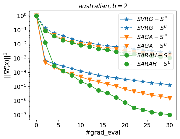
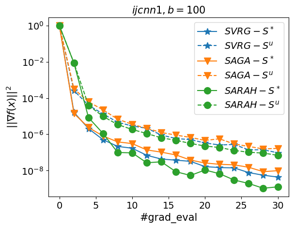
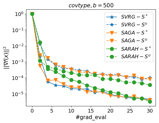
Figure 1: Comparison of all methods with uniform and importance sampling: gradient norm.

5 Experiments

In this section, we perform experiments with regression for binary classification, where our loss function has the form

$$f(x)=\frac{1}{n}\sum_{i=1}^{n}(1-y_{i}\sigma(a_{i}^{\top}x))^{2},$$

where $\sigma(z)$ is the sigmoid function. Hence, $f$ is smooth but non-convex. We chose this function because $L_{i}$’s can be easily computed (however, in many cases, even for much more complex problems, they can usually be estimated). We use four LIBSVM datasets: covtype, ijcnn1, splice, australian.

Parameters of each algorithm are chosen as suggested by the theorems in Section 3, and $x^{0}=0$. For SARAH, we chose $m=\lceil n/b\rceil$. The $y$ axis in all plots displays the norm of the gradient ($\|\nabla f(x)\|^{2}$) or the function value $f(x)$, and the $x$ axis depicts either epochs (1 epoch = 1 pass over data) or iterations.

5.1 Importance vs uniform sampling

Here we provide comparison of the methods with uniform ($S^{u}$) and importance ($S^{*}$) sampling. Looking at Figure 1, one can see that importance sampling outperforms uniform sampling for all three methods, in some cases, even by several orders of magnitude. For instance, in the left plot (minibatch size $b=2$ and australian dataset) the improvement is as large as $4$ orders of magnitude.

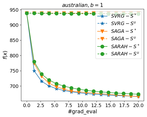
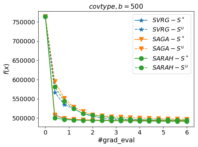
Figure 2: Comparison of all methods with uniform and importance sampling for function values.

Looking at Figure 2, one can see that there is an improvement not just in the norm of the gradient, but also in the function value. In the case of the australian dataset, the constants $L_{i}$’s are very non-uniform, and we can see that the improvement is very significant.

5.2 Linear or superlinear speedup

Our theory suggests that linear or even superlinear speedup (in minibatch size $b$) can be obtained using the optimal independent $S^{*}$. Our experiments show that this is indeed the case in practice as well, and for all three algorithms.

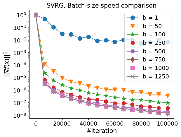
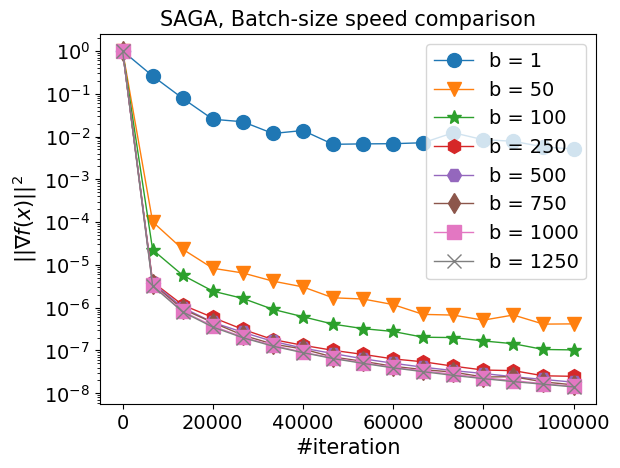
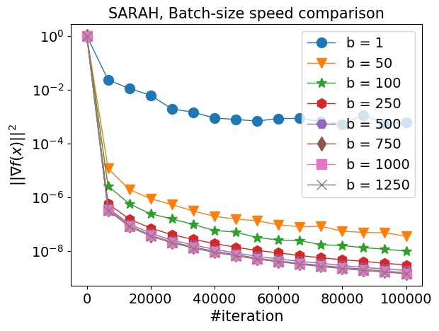
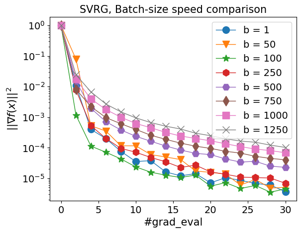
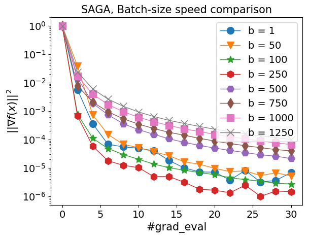
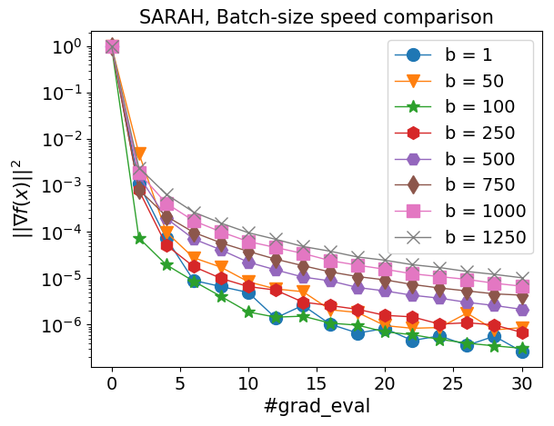
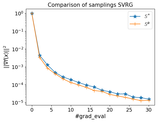
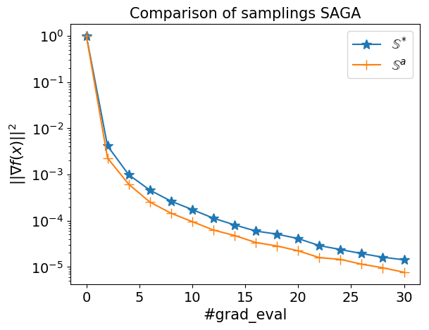
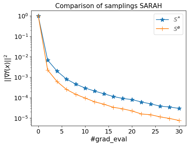
Figure 3: Minibatch speedup, ijcnn1 dataset

Figure 4: Performance of sampling $S^{*}$ vs. $S^{a}$, splice dataset.

Figure 4 confirms that linear, and sometimes even superlinear, speedup is present. For this dataset, such speedup is present up to the minibatch size of $250$. The plots in the top row of Figure 4 depict convergence in a simulated multi-core setting, where the number of cores is the same as the minibatch size.

5.3 Independent vs approximate independent sampling

According to our theory, Independent Sampling $S^{*}$ is slightly better than Approximate Independent Sampling $S^{a}$. However, it is more expensive to use it in practice as generating samples from it involves more computational effort for large $n$.

The goal of our next experiment is to show that in practice $S^{a}$ yields comparable or even faster convergence. Hence, it is more reasonable to use this sampling for datasets where the number of data points $n$ is big. For an efficient implementation of $S^{a}$, we can almost get rid of dependence on $n$. Intuitively, $S^{a}$ works better because it has smaller variance in minibatch size than $S^{*}$.

Indeed, it can be seen from Figure 4 that $S^{a}$ can outperform $S^{*}$ in practice even though $S^{*}$ is optimal in theory. The difference can be small (the left and the middle plot), but also quite significant (right plot).

Supplementary Material

Appendix A Proof of Lemma 1

Proof.

Let $1_{i\in S}=1$ if $i\in S$ and $1_{i\in S}=0$ otherwise. Likewise, let $1_{i,j\in S}=1$ if $i,j\in S$ and $1_{i,j\in S}=0$ otherwise. Note that ${{\rm E}}\left[1_{i\in S}\right]=p_{i}$ and ${{\rm E}}\left[1_{i,j\in S}\right]=p_{ij}$. Next, let us compute the mean of $X:=\sum_{i\in S}\frac{\zeta_{i}}{np_{i}}$:

$${{\rm E}}\left[X\right]={{\rm E}}\left[\sum_{i\in S}\frac{\zeta_{i}}{np_{i}}\right]={{\rm E}}\left[\sum_{i=1}^{n}\frac{\zeta_{i}}{np_{i}}1_{i\in S}\right]=\sum_{i=1}^{n}\frac{\zeta_{i}}{np_{i}}{{\rm E}}\left[1_{i\in S}\right]=\frac{1}{n}\sum_{i=1}^{n}\zeta_{i}=\bar{\zeta}.$$ (11)

Let ${\bf A}=[a_{1},\dots,a_{n}]\in\mathbb{R}^{d\times n}$, where $a_{i}=\frac{\zeta_{i}}{p_{i}}$, and let $e$ be the vector of all ones in $\mathbb{R}^{n}$. We now write the variance of $X$ in a form which will be convenient to establish a bound:

$${{\rm E}}\left[\left\|X-{{\rm E}}\left[X\right]\right\|^{2}\right] = {{\rm E}}\left[\lVert X\rVert^{2}\right]-\|{{\rm E}}\left[X\right]\|^{2}$$ (12)

$$= {{\rm E}}\left[\left\|\sum_{i\in S}\frac{\zeta_{i}}{np_{i}}\right\|^{2}\right]-\lVert\bar{\zeta}\rVert^{2}$$

$$= {{\rm E}}\left[\sum_{i,j}\frac{\zeta_{i}^{\top}}{np_{i}}\frac{\zeta_{j}}{np_{j}}1_{i,j\in S}\right]-\lVert\bar{\zeta}\rVert^{2}$$

$$= \sum_{i,j}p_{ij}\frac{\zeta_{i}^{\top}}{np_{i}}\frac{\zeta_{j}}{np_{j}}-\sum_{i,j}\frac{\zeta_{i}^{\top}}{n}\frac{\zeta_{j}}{n}$$

$$= \frac{1}{n^{2}}\sum_{i,j}(p_{ij}-p_{i}p_{j})a_{i}^{\top}a_{j}$$

$$= \frac{1}{n^{2}}e^{\top}\left(\left({\bf P}-pp^{\top}\right)\circ{\bf A}^{\top}{\bf A}\right)e.$$

Since by assumption we have ${\bf P}-pp^{\top}\preceq\mathbf{Diag}\left(p\circ v\right)$, we can further bound

$$e^{\top}\left(\left({\bf P}-pp^{\top}\right)\circ{\bf A}^{\top}{\bf A}\right)e\leq e^{\top}\left(\mathbf{Diag}\left(p\circ v\right)\circ{\bf A}^{\top}{\bf A}\right)e=\sum_{i=1}^{n}p_{i}v_{i}\|a_{i}\|^{2}.$$

To obtain (5), it remains to combine this with (12).

Inequality (6) follows by comparing the diagonal elements of the two matrices in (4). Let us now verify the formulas for $v$.

• Since ${\bf P}-pp^{\top}$ is positive semidefinite [Richtárik and Takáč, 2016b], we can bound ${\bf P}-pp^{\top}\preceq n\mathbf{Diag}\left({\bf P}-pp^{\top}\right)=\mathbf{Diag}\left(p\circ v\right)$, where $v_{i}=n(1-p_{i})$.

• It was shown by Qu and Richtárik [2016, Theorem 4.1] that ${\bf P}\preceq d\mathbf{Diag}\left(p\right)$ provided that $|S|\leq d$ with probability 1. Hence, ${\bf P}-pp^{\top}\preceq{\bf P}\preceq d\mathbf{Diag}\left(p\right)$, which means that $v_{i}=d$ for all $i$.

• Consider now the independent sampling. Clearly,

  $${\bf P}-pp^{\top}=\begin{bmatrix}p_{1}(1-p_{1})&0&\dots&0\\ 0&p_{2}(1-p_{2})&\dots&0\\ \vdots&\vdots&\ddots&\vdots\\ 0&0&\dots&p_{n}(1-p_{n})\end{bmatrix}=\mathbf{Diag}\left(p_{1}v_{1},\dots,p_{n}v_{n}\right),$$

  where $v_{i}=1-p_{i}$.

• Consider the $b$–nice sampling (standard uniform minibatch sampling). Direct computation shows that the probability matrix is given by

  $${\bf P}=\begin{bmatrix}\tfrac{b}{n}&\tfrac{b(b-1)}{n(n-1)}&\dots&\tfrac{b(b-1)}{n(n-1)}\\ \tfrac{b(b-1)}{n(n-1)}&\tfrac{b}{n}&\dots&\tfrac{b(b-1)}{n(n-1)}\\ \vdots&\vdots&\ddots&\vdots\\ \tfrac{b(b-1)}{n(n-1)}&\tfrac{b(b-1)}{n(n-1)}&\dots&\tfrac{b}{n}\end{bmatrix},$$

  as claimed in (3). Therefore,

  $${\bf P}-pp^{\top}=\begin{bmatrix}\tfrac{b}{n}-\frac{b^{2}}{n^{2}}&\tfrac{b(b-1)}{n(n-1)}&\dots&\tfrac{b(b-1)}{n(n-1)}\\ \tfrac{b(b-1)}{n(n-1)}&\tfrac{b}{n}&\dots&\tfrac{b(b-1)}{n(n-1)}\\ \vdots&\vdots&\ddots&\vdots\\ \tfrac{b(b-1)}{n(n-1)}&\tfrac{b(b-1)}{n(n-1)}&\dots&\tfrac{b}{n}\end{bmatrix},$$

• Letting $t=\frac{(a-1)k}{a(k-1)}$ and $s=1-t=\tfrac{k-a}{a(k-1)}$ the probability matrix of the approximate independent sampling satisfies

  $${\bf P}-pp^{\top} = \begin{bmatrix}p_{1}(1-p_{1})&(t-1)p_{1}p_{2}&\dots&(t-1)p_{1}p_{k}&0&\dots&0\\ (t-1)p_{2}p_{1}&p_{2}(1-p_{2})&\dots&(t-1)p_{2}p_{k}&0&\dots&0\\ \vdots&\vdots&\ddots&\vdots&0&\dots&0\\ (t-1)p_{n}p_{1}&(t-1)p_{n}p_{2}&\dots&p_{k}(1-p_{k})&0&\dots&0\\ 0&0&\dots&0&0&\dots&0\\ \vdots&\vdots&\vdots&\vdots&\vdots&\ddots&\vdots\\ 0&0&\dots&0&0&\dots&0\end{bmatrix}$$

  $$= \mathbf{Diag}\left(p_{1}(1-p_{1}(1-s)),\dots,p_{k}(1-p_{k}(1-s)),0,\dots,0\right)-sp_{k}p_{k}^{\top}$$

  $$\preceq \mathbf{Diag}\left(p_{1}(1-p_{1}(1-s)),\dots,p_{n}(1-p_{n}(1-s)),0,\dots,0\right),$$

  where $p_{k}=(p_{1},\dots,p_{k},0,\dots,0)^{\top}.$ Therefore, $v_{i}=1-p_{i}(1-s)$ for $i\leq k$ and $v_{i}=0$ otherwise works.

• Finally, as remarked in the introduction, the standard uniform minibatch sampling ($b$–nice sampling) arises as a special case of the approximate independent sampling for the choice $p_{i}=b/n$. Thus $k=n,$ $a=b$ and hence $s=\tfrac{n-b}{b(n-1)}$. Based on the previous result, $v_{i}=1-\tfrac{b}{n}(1-\tfrac{n-b}{b(n-1)})=\frac{n-b}{n-1}$ works.

∎

Appendix B Proof of Theorem 2

We first establish a lemma we will need in order to prove Theorem 2.

Lemma 6.

Let $0<L_{1}\leq L_{2}\leq\dots\leq L_{n}$ be positive real numbers, $0<b\leq n$, and consider the optimization problem

$$\text{minimize}_{p\in\mathbb{R}^{n}} \Omega(p):=\sum_{i=1}^{n}\frac{L_{i}^{2}}{p_{i}}$$

subject to $$\sum_{i=1}^{n}p_{i}=b,$$

$$0\leq p_{i}\leq 1,\quad i=1,2,\dots,n.$$

Let be the largest integer for which $0<b+k-n\leq\frac{\sum_{i=1}^{k}L_{i}}{L_{k}}$ (note that the inequality holds for $k=n-b+1$). Then (6) has the following solution:

$$p_{i}=\begin{cases}(b+k-n)\frac{L_{i}}{\sum_{j=1}^{k}L_{j}},&\quad\text{if }i\leq k,\\ 1,&\quad\text{if }i>k.\end{cases}$$ (14)

Proof.

The Lagrangian of the problem is

$$L(p,y,\lambda_{1},..,\lambda_{n},u_{1},...,u_{n})=\sum_{i=1}^{n}\frac{L_{i}^{2}}{p_{i}}-\sum_{i=1}^{n}\lambda_{i}p_{i}-\sum_{i=1}^{n}u_{i}(1-p_{i})+y\left(\sum_{i=1}^{n}p_{i}-b\right).$$

Th constraints are linear and hence KKT conditions hold. The result can be deduced from the KKT conditions. ∎

We can now proceed with the proof. Since $n,b$ and $\bar{L}$ are constants, the problem is equivalent to

$$\text{minimize}_{S} \psi(S):=\sum_{i=1}^{n}\frac{v_{i}L_{i}^{2}}{p_{i}}$$

subject to $$v_{i}\quad\text{satisfies}\quad\eqref{eq:ESO}.$$

In view of (6),

$$\psi(S)\overset{\eqref{v_i}}{\geq}\sum_{i=1}^{n}\frac{(1-p_{i})L_{i}^{2}}{p_{i}}=\sum_{i=1}^{n}\frac{L_{i}^{2}}{p_{i}}-\sum_{i=1}^{n}L_{i}^{2}=\Omega(p)-\sum_{i=1}^{n}L_{i}^{2},$$

where function $\Omega(p)$ was defined in Lemma 6. Since $b={{\rm E}}\left[|S|\right]=\sum_{i}p_{i}$, and $0\leq p_{i}\leq 1$ for all $i$, then in view of Lemma 6 we have

$$\Psi(S)\geq\Omega(p^{*})-\sum_{i=1}^{n}L_{i}^{2},$$

where $p^{*}$ is defined by (8).

On the other hand, from Lemma 1 we know that the independent sampling $S=S^{*}$ with probability vector $p^{*}$ defined in (8) satisfies inequality (4) with $v_{i}=1-p_{i}$, and hence

$$\Psi(S^{*})=\Omega(p^{*})-\sum_{i=1}^{n}L_{i}^{2}.$$

Hence, it is optimal. ∎

Appendix C Improvements

Let us compute $\alpha$ for uniform sampling.

$$\alpha \overset{\eqref{def_K}}{=} \left(\frac{b}{n^{2}}\sum_{i=1}^{n}\frac{v_{i}L_{i}^{2}}{p_{i}}\right)/\bar{L}^{2}$$

$$\overset{\text{Lemma}~{}\ref{lem:upperv}}{=} \left(\frac{(n-b)}{(n-1)n}\sum_{i=1}^{n}L_{i}^{2}\right)/\bar{L}^{2}$$

$$= n\frac{(n-b)}{(n-1)}\sum_{i=1}^{n}L_{i}^{2}/\left(\sum_{i=1}^{n}L_{i}\right)^{2}$$

It is easy to see that $L_{\max}\geq\bar{L}$. To prove that we have improved current best known rates, we need to show that $\bar{L}\alpha\leq L_{\max}$ and $\bar{L}^{2}\alpha\leq\frac{(n-b)}{(n-1)}L_{\max}^{2}$

Proof.

$$\bar{L}\alpha = n\frac{(n-b)}{(n-1)}\frac{\sum_{i=1}^{n}L_{i}^{2}}{\left(\sum_{i=1}^{n}L_{i}\right)^{2}}\bar{L}\leq\frac{\sum_{i=1}^{n}L_{i}^{2}}{\left(\sum_{i=1}^{n}L_{i}\right)}=\frac{\sum_{i=1}^{n}L_{\max}L_{i}}{\left(\sum_{i=1}^{n}L_{i}\right)}=L_{\max},$$

$$\bar{L}^{2}\alpha = n\frac{(n-b)}{(n-1)}\frac{\sum_{i=1}^{n}L_{i}^{2}}{\left(\sum_{i=1}^{n}L_{i}\right)^{2}}\bar{L}^{2}=\frac{(n-b)}{(n-1)}\frac{1}{n}\sum_{i=1}^{n}L_{i}^{2}\leq\frac{(n-b)}{(n-1)}\frac{1}{n}\sum_{i=1}^{n}L_{\max}^{2}=\frac{(n-b)}{(n-1)}L_{\max}^{2},$$

∎

Let’s take $b=1$. If $L_{n}\gg L_{i},\forall i\in[n]$, then $L_{\max}\approx n\bar{L}$ and $\alpha_{S^{*}}\leq 1$ and $\alpha_{S^{u}}\approx n$, which essentially means, that we can have in theory speedup by factor of $n$.

Appendix D Stochastic gradients evaluation complexity

D.1 SVRG

For SVRG, each outer loop costs $n+mb$ evaluations of stochastic gradient. If we want to obtain $\epsilon$-solution, following must hold (Theorem 3)

$$\frac{\alpha\bar{L}n^{(2/3)}(f(x^{0})-f(x^{*}))}{bMm\nu_{2}}\leq\epsilon$$

Combining these two equations with definition from Theorem 3, we get total complexity in terms of stochastic gradients evaluation

$$\frac{\mu_{2}\bar{L}n^{(2/3)}(f(x^{0})-f(x^{*}))}{\epsilon\nu_{2}}(1+\frac{\alpha}{3\mu_{2}})$$

D.2 SAGA

For SAGA, each loop costs $d+b$ evaluations of stochastic gradient. If we want to obtain $\epsilon$-solution, following must hold (Theorem 4)

$$\frac{\alpha\bar{L}n^{(2/3)}(f(x^{0})-f(x^{*}))}{bT\nu_{2}}\leq\epsilon$$

Combining these two equations with definition from Theorem 4, we get total complexity in terms of stochastic gradients evaluation

$$n+\frac{\bar{L}n^{(2/3)}(f(x^{0})-f(x^{*}))}{\epsilon\nu_{3}}(1+\alpha),$$

because of evaluation of full gradient on the start.

D.3 SARAH

For SARAH with one outer loot, each inner loop costs $2b$ evaluations of stochastic gradient. If we want to obtain $\epsilon$-solution, following must hold (Theorem 5)

$$\frac{2\bar{L}(f(x^{0})-f(x^{*}))\left(\sqrt{1+\frac{4m\alpha}{b}}\right)}{m}\leq\epsilon$$

Solving this equation for $m$, we get

$$m\leq\frac{16\alpha\bar{L}^{2}(f(x^{0})-f(x^{*}))^{2}+\sqrt{16^{2}\alpha^{2}\bar{L}^{4}(f(x^{0})-f(x^{*}))^{4}+16\epsilon^{2}\bar{L}^{2}(f(x^{0})-f(x^{*}))^{2}b^{2}}}{2b\epsilon^{2}}$$

Combining thise equation with complexity off each inner loop we obtain total complexity in terms of stochastic gradients evaluation

$$\frac{16\alpha\bar{L}^{2}(f(x^{0})-f(x^{*}))^{2}+\sqrt{16^{2}\alpha^{2}\bar{L}^{4}(f(x^{0})-f(x^{*}))^{4}+16\epsilon^{2}\bar{L}^{2}(f(x^{0})-f(x^{*}))^{2}b^{2}}}{2\epsilon^{2}}.$$

Appendix E Proofs for SVRG

Lemma 7.

For $c_{t},c_{t+1},\beta>0$, suppose we have

$$c_{t}=c_{t+1}(1+\eta\beta+2\eta^{2}K)+K\eta^{2}\bar{L}.$$

Let $\eta$, $\beta$ and $c_{t+1}$ be chosen such that $\Gamma_{t}>0$ (in Theorem (17)). The iterate $x^{s+1}_{t}$ in Algorithm 5 satisfy the bound:

$${{\rm E}}\left[\|\nabla f(x^{s+1}_{t})\|^{2}\right]\leq\frac{R^{s+1}_{t}-R^{s+1}_{t+1}}{\Gamma_{t}},$$

where $R^{s+1}_{t}:={{\rm E}}\left[f(x^{s+1}_{t})+c_{t}\|x^{s+1}_{t}-\tilde{x}^{s}\|^{2}\right]$ for $0\leq s\leq S-1$.

Proof.

Since $f_{i}$ is $L_{i}$-smooth we have

$${{\rm E}}\left[f_{i}(x^{s+1}_{t+1})\right]\leq{{\rm E}}\left[f_{i}(x^{s+1}_{t})+\langle\nabla f_{i}(x^{s+1}_{t}),x^{s+1}_{t+1}-x^{s+1}_{t}\rangle+\tfrac{L_{i}}{2}\|x^{s+1}_{t+1}-x^{s+1}_{t}\|^{2}\right].$$

Summing through all $i$ and dividing by $n$ we obtain

$${{\rm E}}\left[f(x^{s+1}_{t+1})\right]\leq{{\rm E}}\left[f(x^{s+1}_{t})+\langle\nabla f(x^{s+1}_{t}),x^{s+1}_{t+1}-x^{s+1}_{t}\rangle+\tfrac{\bar{L}}{2}\|x^{s+1}_{t+1}-x^{s+1}_{t}\|^{2}\right].$$

Using the SVRG update in Algorithm 5 and its unbiasedness (${{\rm E}}\left[i_{t}\right]{v^{s+1}_{t}}=\nabla f(x_{t}^{s+1})$), the right hand side above is further upper bounded by

$${{\rm E}}\left[f(x^{s+1}_{t})-\eta\|\nabla f(x^{s+1}_{t})\|^{2}+\tfrac{\bar{L}\eta^{2}}{2}\|v^{s+1}_{t}\|^{2}\right].$$ (15)

Consider now the Lyapunov function

$$R^{s+1}_{t}:={{\rm E}}\left[f(x^{s+1}_{t})+c_{t}\|x^{s+1}_{t}-\tilde{x}^{s}\|^{2}\right].$$

For bounding it we will require the following:

$${{\rm E}}\left[\|x^{s+1}_{t+1}-\tilde{x}^{s}\|^{2}\right] = {{\rm E}}\left[\|x^{s+1}_{t+1}-x^{s+1}_{t}+x^{s+1}_{t}-\tilde{x}^{s}\|^{2}\right]$$ (16)

$$= {{\rm E}}\left[\|x^{s+1}_{t+1}-x^{s+1}_{t}\|^{2}+\|x^{s+1}_{t}-\tilde{x}^{s}\|^{2}\right]$$

$$\quad+2\langle x^{s+1}_{t+1}-x^{s+1}_{t},x^{s+1}_{t}-\tilde{x}^{s}\rangle]$$

$$= {{\rm E}}\left[\eta^{2}\|v^{s+1}_{t}\|^{2}+\|x^{s+1}_{t}-\tilde{x}^{s}\|^{2}\right]$$

$$\quad-2\eta{{\rm E}}\left[\langle\nabla f(x^{s+1}_{t}),x^{s+1}_{t}-\tilde{x}^{s}\rangle\right]$$

$$\overset{\eqref{CS},\eqref{Young}}{\leq} {{\rm E}}\left[\eta^{2}\|v^{s+1}_{t}\|^{2}+\|x^{s+1}_{t}-\tilde{x}^{s}\|^{2}\right]$$

$$\qquad+2\eta{{\rm E}}\left[\tfrac{1}{2\beta}\|\nabla f(x^{s+1}_{t})\|^{2}+\tfrac{1}{2}\beta\|x^{s+1}_{t}-\tilde{x}^{s}\|^{2}\right].$$

The second equality follows from the unbiasedness of the update of SVRG. Plugging Equation (15) and Equation (16) into $R^{s+1}_{t+1}$, we obtain the following bound:

$$R^{s+1}_{t+1} \leq {{\rm E}}\left[f(x^{s+1}_{t})-\eta\|\nabla f(x^{s+1}_{t})\|^{2}+\tfrac{\bar{L}\eta^{2}}{2}\|v^{s+1}_{t}\|^{2}\right]$$ (17)

$$\quad+{{\rm E}}\left[c_{t+1}\eta^{2}\|v^{s+1}_{t}\|^{2}+c_{t+1}\|x^{s+1}_{t}-\tilde{x}^{s}\|^{2}\right]$$

$$\quad+2c_{t+1}\eta{{\rm E}}\left[\tfrac{1}{2\beta}\|\nabla f(x^{s+1}_{t})\|^{2}+\tfrac{1}{2}\beta\|x^{s+1}_{t}-\tilde{x}^{s}\|^{2}\right]$$

$$\leq {{\rm E}}\left[f(x^{s+1}_{t})-\left(\eta-\tfrac{c_{t+1}\eta}{\beta}\right)\|\nabla f(x^{s+1}_{t})\|^{2}\right]+\left(\tfrac{\bar{L}\eta^{2}}{2}+c_{t+1}\eta^{2}\right){{\rm E}}\left[\|v^{s+1}_{t}\|^{2}\right]$$

$$\quad+\left(c_{t+1}+c_{t+1}\eta\beta\right){{\rm E}}\left[\|x^{s+1}_{t}-\tilde{x}^{s}\|^{2}\right].$$

To further bound this quantity, we use Lemma 10 to bound ${{\rm E}}\left[\|v^{s+1}_{t}\|^{2}\right]$, so that upon substituting it in Equation (17), we see that

$$R^{s+1}_{t+1} \overset{\eqref{nonconvex-variance-lemma}}{\leq} {{\rm E}}\left[f(x^{s+1}_{t})\right]-\left(\eta-\tfrac{c_{t+1}\eta}{\beta}-\eta^{2}\bar{L}-2c_{t+1}\eta^{2}\right){{\rm E}}\left[\|\nabla f(x^{s+1}_{t})\|^{2}\right]$$ (18)

$$\qquad+\left[c_{t+1}\bigl{(}1+\eta\beta+2\eta^{2}K\bigr{)}+\eta^{2}K\bar{L}\right]{{\rm E}}\left[\|x^{s+1}_{t}-\tilde{x}^{s}\|^{2}\right]$$

$$\leq R^{s+1}_{t}-\bigl{(}\eta-\tfrac{c_{t+1}\eta}{\beta}-\eta^{2}\bar{L}-2c_{t+1}\eta^{2}\bigr{)}{{\rm E}}\left[\|\nabla f(x^{s+1}_{t})\|^{2}\right].$$

The second inequality follows from the definition of $c_{t}$ and $R_{t}^{s+1}$, thus concluding the proof. ∎

Proof of Lemma 7 and Theorem 17

Proof.

Using Lemma 7 and telescoping the sum, we obtain

$$\sum_{t=0}^{m-1}{{\rm E}}\left[\|\nabla f(x^{s+1}_{t})\|^{2}\right]\leq\frac{R^{s+1}_{0}-R^{s+1}_{m}}{\gamma_{n}}.$$ (19)

This inequality in turn implies that

$$\sum_{t=0}^{m-1}{{\rm E}}\left[\|\nabla f(x^{s+1}_{t})\|^{2}\right]\leq\frac{{{\rm E}}\left[f(\tilde{x}^{s})-f(\tilde{x}^{s+1})\right]}{\gamma_{n}},$$ (20)

where we used that $R^{s+1}_{m}={{\rm E}}\left[f(x^{s+1}_{m})\right]={{\rm E}}\left[f(\tilde{x}^{s+1})\right]$ (since $c_{m}=0$), and that $R^{s+1}_{0}={{\rm E}}\left[f(\tilde{x}^{s})\right]$ (since $x^{s+1}_{0}=\tilde{x}^{s}$). Now sum over all epochs to obtain

$$\frac{1}{T}\sum_{s=0}^{S-1}\sum_{t=0}^{m-1}{{\rm E}}\left[\|\nabla f(x^{s+1}_{t})\|^{2}\right]\leq\frac{f(x^{0})-f(x^{*})}{T\gamma_{n}}.$$ (21)

The above inequality used the fact that $\tilde{x}^{0}=x^{0}$. Using the above inequality and the definition of $x_{a}$ in Algorithm 5, we obtain the desired result. ∎

Proof of Theorem 18

Proof.

For our analysis, we will require an upper bound on $c_{0}$. Let $m=\lfloor Kn/(3\bar{L}^{2}\rfloor\mu_{0}),\eta=\mu_{0}\bar{L}/(Kn^{2/3}).$ We observe that $c_{0}=\tfrac{\mu_{0}^{2}\bar{L}^{3}}{Kn^{4/3}}\tfrac{(1+\theta)^{m}-1}{\theta}$ where $\theta=2K\eta^{2}+\eta\beta$. This is obtained using the relation $c_{t}=c_{t+1}(1+\eta\beta+2K\eta^{2})+\eta^{2}K\bar{L}$ and the fact that $c_{m}=0$. Using the specified values of $\beta$ and $\eta$ we have

$$\theta=2K\eta^{2}+\eta\beta=\frac{2\mu_{0}^{2}\bar{L}^{2}}{Kn^{4/3}}+\frac{\mu_{0}\bar{L}^{2}}{Kn}\leq\frac{3\mu_{0}\bar{L}^{2}}{Kn}.$$ (22)

The above inequality follows since $\mu_{0}\leq 1$ and $n\geq 1$. Using the above bound on $\theta$, we get

$$c_{0} = \frac{\mu_{0}^{2}\bar{L}^{3}}{n^{2}K}\frac{(1+\theta)^{m}-1}{\theta}=\frac{\mu_{0}\bar{L}((1+\theta)^{m}-1)}{2\mu_{0}+n^{\tfrac{1}{3}}}$$ (23)

$$\leq \frac{\mu_{0}\bar{L}((1+\frac{3\mu_{0}\bar{L}^{2}}{nK})^{\lfloor\nicefrac{{Kn}}{{3\mu_{0}\bar{L}^{2}}}\rfloor}-1)}{2\mu_{0}+n^{\tfrac{1}{3}}}$$

$$\leq n^{-\tfrac{1}{3}}(\mu_{0}\bar{L}(e-1)),$$

wherein the second inequality follows upon noting that $(1+\frac{1}{l})^{l}$ is increasing for $l>0$ and $\lim_{l\rightarrow\infty}(1+\frac{1}{l})^{l}=e$ (here $e$ is the Euler’s number). Now we can lower bound $\gamma_{n}$, as

$$\gamma_{n} =\min_{t}\bigl{(}\eta-\tfrac{c_{t+1}\eta}{\beta}-\eta^{2}\bar{L}-2c_{t+1}\eta^{2}\bigr{)}$$

$$\geq\bigl{(}\eta-\tfrac{c_{0}\eta}{\beta}-\eta^{2}\bar{L}-2c_{0}\eta^{2}\bigr{)}\geq\frac{\nu\bar{L}}{Kn^{\tfrac{2}{3}}},$$

where $\nu$ is a constant independent of $n$. The first inequality holds since $c_{t}$ decreases with $t$. The second inequality holds since (a) $c_{0}/\beta$ is upper bounded by a constant independent of $n$ as $c_{0}/\beta\leq\mu_{0}(e-1)$ (follows from Equation (23)), (b) $\eta^{2}\bar{L}\leq\mu_{0}\eta$ and (c) $2c_{0}\eta^{2}\leq 2\mu_{0}^{2}(e-1)\eta$ (follows from Equation (23)). By choosing $\mu_{0}$ (independent of $n$) appropriately, one can ensure that $\gamma_{n}\geq\nu\bar{L}/(Kn^{\tfrac{2}{3}})$ for some universal constant $\nu$. For example, choosing $\mu_{0}=1/4$, we have $\gamma_{n}\geq\nu\bar{L}/(Kn^{\tfrac{2}{3}})$ with $\nu=1/40$. Substituting the above lower bound in Equation (21), we obtain the desired result. ∎

Appendix F Minibatch SVRG

Proof of Theorem 3

The proofs essentially follow along the lines of Lemma 7, Theorem 17 and Theorem 18 with the added complexity of mini-batch. We first prove few intermediate results before proceeding to the proof of Theorem 3.

Lemma 8.

Suppose we have

$$\overline{R}^{s+1}_{t}:={{\rm E}}\left[f(x^{s+1}_{t})+\overline{c}_{t}\|x^{s+1}_{t}-\tilde{x}^{s}\|^{2}\right],$$ (25)

$$\overline{c}_{t}=\overline{c}_{t+1}(1+\eta\beta+\frac{2K\eta^{2}}{b})+\frac{K\eta^{2}\bar{L}}{b},$$

for $\ 0\leq s\leq S-1$ and $0\leq t\leq m-1$ and the parameters $\eta,\beta$ and $\overline{c}_{t+1}$ are chosen such that

$$\left(\eta-\frac{\overline{c}_{t+1}\eta}{\beta}-\eta^{2}\bar{L}-2\overline{c}_{t+1}\eta^{2}\right)\geq 0.$$

Then the iterates $x^{s+1}_{t}$ in the mini-batch version of Algorithm 5 i.e., Algorithm 1 with expected mini-batch size $b$ satisfy the bound:

$${{\rm E}}\left[\|\nabla f(x^{s+1}_{t})\|^{2}\right]\leq\frac{\overline{R}^{s+1}_{t}-\overline{R}^{s+1}_{t+1}}{\left(\eta-\frac{\overline{c}_{t+1}\eta}{\beta}-\eta^{2}\bar{L}-2\overline{c}_{t+1}\eta^{2}\right)},$$

Proof.

Using essentially the same argument as the proof of Lemma 7 until Equation (17), we have

$$\overline{R}^{s+1}_{t+1} \leq {{\rm E}}\left[(x^{s+1}_{t})\right]-\left(\eta-\tfrac{\overline{c}_{t+1}\eta}{\beta}\right)\|\nabla f(x^{s+1}_{t})\|^{2}+\left(\tfrac{\bar{L}\eta^{2}}{2}+\overline{c}_{t+1}\eta^{2}\right){{\rm E}}\left[\|v^{s+1}_{t}\|^{2}\right]$$ (26)

$$\quad+\left(\overline{c}_{t+1}+\overline{c}_{t+1}\eta\beta\right){{\rm E}}\left[\|x^{s+1}_{t}-\tilde{x}^{s}\|^{2}\right].$$

We use Lemma 11 in order to bound ${{\rm E}}\left[\|v^{s+1}_{t}\|^{2}\right]$ in the above inequality. Substituting it in Equation (26), we see that

$$\overline{R}^{s+1}_{t+1} \overset{\eqref{nonconvex-variance-lemma_b}}{\leq} {{\rm E}}\left[f(x^{s+1}_{t})\right]-\left(\eta-\tfrac{\overline{c}_{t+1}\eta}{\beta}-\eta^{2}\bar{L}-2\overline{c}_{t+1}\eta^{2}\right){{\rm E}}\left[\|\nabla f(x^{s+1}_{t})\|^{2}\right]$$ (27)

$$\quad+\left[\overline{c}_{t+1}\bigl{(}1+\eta\beta+\tfrac{2K\eta^{2}}{b}\bigr{)}+\tfrac{K\eta^{2}\bar{L}}{b}\right]{{\rm E}}\left[\|x^{s+1}_{t}-\tilde{x}^{s}\|^{2}\right]$$

$$\overset{\eqref{n312412asd}}{\leq} \overline{R}^{s+1}_{t}-\bigl{(}\eta-\tfrac{\overline{c}_{t+1}\eta}{\beta}-\eta^{2}\bar{L}-2\overline{c}_{t+1}\eta^{2}\bigr{)}{{\rm E}}\left[\|\nabla f(x^{s+1}_{t})\|^{2}\right].$$

The second inequality follows from the definition of $\overline{c}_{t}$ and $\overline{R}^{s+1}_{t}$, thus concluding the proof. ∎

The following theorem provides convergence rate of mini-batchSVRG.

Theorem 9.

Let $\overline{\gamma}_{n}$ denote the following quantity:

$$\overline{\gamma}_{n}:=\min_{0\leq t\leq m-1}\quad\bigl{(}\eta-\tfrac{\overline{c}_{t+1}\eta}{\beta}-\eta^{2}\bar{L}-2\overline{c}_{t+1}\eta^{2}\bigr{)}.$$

Suppose $\overline{c}_{m}=0$, $\overline{c}_{t}=\overline{c}_{t+1}(1+\eta\beta+\frac{2K\eta^{2}}{b})+\frac{K\eta^{2}\bar{L}}{b}$ for $t\in\{0,\dots,m-1\}$ and $\overline{\gamma}_{n}>0$. Then for the output $x_{a}$ of mini-batch version of Algorithm 5 with mini-batch size $b$, we have

$${{\rm E}}\left[\|\nabla f(x_{a})\|^{2}\right]\leq\frac{f(x^{0})-f(x^{*})}{T\overline{\gamma}_{n}},$$

where $x^{*}$ is an optimal solution to (1).

Proof.

Using Lemma 8 and telescoping the sum, we obtain

$$\sum_{t=0}^{m-1}{{\rm E}}\left[\|\nabla f(x^{s+1}_{t})\|^{2}\right]\leq\frac{\overline{R}^{s+1}_{0}-\overline{R}^{s+1}_{m}}{\overline{\gamma}_{n}}.$$

This inequality in turn implies that

$$\sum_{t=0}^{m-1}{{\rm E}}\left[\|\nabla f(x^{s+1}_{t})\|^{2}\right]\leq\frac{{{\rm E}}\left[f(\tilde{x}^{s})-f(\tilde{x}^{s+1})\right]}{\overline{\gamma}_{n}},$$

where we used that $\overline{R}^{s+1}_{m}={{\rm E}}\left[f(x^{s+1}_{m})\right]={{\rm E}}\left[f(\tilde{x}^{s+1})\right]$ (since $\overline{c}_{m}=0$), and that $\overline{R}^{s+1}_{0}={{\rm E}}\left[f(\tilde{x}^{s})\right]$. Now sum over all epochs and using the fact that $\tilde{x}^{0}=x^{0}$, we get the desired result. ∎

We now present the proof of Theorem 3 using the above results.

Proof of Theorem 3.

We first observe that using the specified values of $\beta=\bar{L}/n^{1/3}$, $\eta=\mu_{2}b\bar{L}/(Kn^{2/3})$ and $\eta=\lfloor nK/(b\bar{L}^{2}\mu_{2})\rfloor$we obtain

$$\overline{\theta}:=\frac{2K\eta^{2}}{b}+\eta\beta=\frac{2\mu_{2}^{2}b\bar{L}^{2}}{Kn^{4/3}}+\frac{\bar{L}^{2}\mu_{2}b}{Kn}\leq\frac{3\mu_{2}\bar{L}^{2}b}{Kn}.$$

The above inequality follows since $\mu_{2}\leq 1$ and $n\geq 1$. For our analysis, we will require the following bound on $\overline{c}_{0}$:

$$\overline{c}_{0} = \frac{\mu_{2}^{2}b^{2}\bar{L}^{3}}{Kbn^{4/3}}\frac{(1+\overline{\theta})^{m}-1}{\overline{\theta}}=\frac{\mu_{2}b\bar{L}((1+\overline{\theta})^{m}-1)}{2b\mu_{2}+bn^{1/3}}$$ (28)

$$\leq n^{-1/3}(\mu_{2}\bar{L}(e-1)),$$

wherein the first equality holds due to the relation $\overline{c}_{t}=\overline{c}_{t+1}(1+\eta\beta+\tfrac{2K\eta^{2}}{b})+\tfrac{K\eta^{2}\bar{L}}{b}$, and the inequality follows upon again noting that $(1+1/l)^{l}$ is increasing for $l>0$ and $\lim_{l\rightarrow\infty}(1+\frac{1}{l})^{l}=e$. Now we can lower bound $\overline{\gamma}_{n}$, as

$$\overline{\gamma}_{n} = \min_{t}\bigl{(}\eta-\tfrac{\overline{c}_{t+1}\eta}{\beta}-\eta^{2}\bar{L}-2\overline{c}_{t+1}\eta^{2}\bigr{)}$$

$$\geq \bigl{(}\eta-\tfrac{\overline{c}_{0}\eta}{\beta}-\eta^{2}\bar{L}-2\overline{c}_{0}\eta^{2}\bigr{)}\geq\frac{b\bar{L}\nu_{2}}{Kn^{2/3}},$$

where $\nu_{2}$ is a constant independent of $n$. The first inequality holds since $\overline{c}_{t}$ decreases with $t$. The second one holds since (a) $\overline{c}_{0}/\beta$ is upper bounded by a constant independent of $n$ as $\overline{c}_{0}/\beta\leq\mu_{2}(e-1)$ (due to Equation(28)), (b) $\eta^{2}\bar{L}\leq\mu_{2}\eta$ (as $b\leq\nicefrac{{K}}{{\bar{L}^{2}n^{2/3}}}$) and (c) $2\overline{c}_{0}\eta^{2}\leq 2\mu_{2}^{2}(e-1)\eta$ (again due to Equation (28) and the fact $b\leq\nicefrac{{K}}{{\bar{L}^{2}n^{2/3}}}$). By choosing an appropriately small constant $\mu_{2}$ (independent of n), one can ensure that $\overline{\gamma}_{n}\geq{\bar{L}b\nu_{2}}/(Kn^{2/3})$ for some universal constant $\nu_{2}$. For example, choosing $\mu_{2}=1/4$, we have $\overline{\gamma}_{n}\geq{\bar{L}b\nu_{2}}/(Kn^{2/3})$ with $\nu_{2}=1/40$. Substituting the above lower bound in Theorem 9, we obtain the desired result. ∎

Lemmas

Lemma 10.

For the intermediate iterates $v^{s+1}_{t}$ computed by Algorithm 5, we have the following:

$${{\rm E}}\left[\|v^{s+1}_{t}\|^{2}\right]\leq 2{{\rm E}}\left[\|\nabla f(x^{s+1}_{t})\|^{2}\right]+2K{{\rm E}}\left[\|x^{s+1}_{t}-\tilde{x}^{s}\|^{2}\right].$$ (29)

Proof.

The proof simply follows from the proof of Lemma 11 with $S_{t}=\{i_{t}\}$. ∎

We now present a result to bound the variance of mini-batch SVRG.

Lemma 11.

Let $v^{s+1}_{t}$ be computed by the mini-batch version of Algorithm 5 i.e., Algorithm 1 with sampling $S$. Then,

$${{\rm E}}\left[\|v^{s+1}_{t}\|^{2}\right]\leq 2{{\rm E}}\left[\|\nabla f(x^{s+1}_{t})\|^{2}\right]+\tfrac{2K}{b}{{\rm E}}\left[\|x^{s+1}_{t}-\tilde{x}^{s}\|^{2}\right].$$ (30)

Proof.

For the simplification, we use the following notation:

$$\zeta_{t}^{s+1}=\sum_{i_{t}\in S_{t}}\frac{1}{np_{i_{t}}}\left(\nabla f_{i_{t}}(x^{s+1}_{t})-\nabla f_{i_{t}}(\tilde{x}^{s})\right).$$

We use the definition of $v^{s+1}_{t}$ to get

$${{\rm E}}\left[\|v^{s+1}_{t}\|^{2}\right] = {{\rm E}}\left[\|\zeta_{t}^{s+1}+\nabla f(\tilde{x}^{s})\|^{2}\right]$$

$$= {{\rm E}}\left[\|\zeta_{t}^{s+1}+\nabla f(\tilde{x}^{s})-\nabla f(x^{s+1}_{t})+\nabla f(x^{s+1}_{t})\|^{2}\right]$$

$$\leq 2{{\rm E}}\left[\|\nabla f(x^{s+1}_{t})\|^{2}\right]+2{{\rm E}}\left[\|\zeta_{t}^{s+1}-{{\rm E}}\left[\zeta_{t}^{s+1}\right]\|^{2}\right]$$

$$= 2{{\rm E}}\left[\|\nabla f(x^{s+1}_{t})\|^{2}\right]$$

$$\quad+2{{\rm E}}\left[\left\|\sum_{i_{t}\in S_{t}}\left(\frac{1}{np_{i_{t}}}\left(\nabla f_{i_{t}}(x^{s+1}_{t})-\nabla f_{i_{t}}(\tilde{x}^{s})\right)-{{\rm E}}\left[\zeta_{t}^{s+1}\right]\right)\right\|^{2}\right].$$

The first inequality follows from fact that $\lVert x+y\rVert^{2}\leq 2\lVert x\rVert^{2}+2\lVert y\rVert^{2}$ and the fact that ${{\rm E}}\left[\zeta_{t}^{s+1}\right]=\nabla f(x^{s+1}_{t})-\nabla f(\tilde{x}^{s})$. From the above inequality, we get

$${{\rm E}}\left[\|v^{s+1}_{t}\|^{2}\right] \overset{\eqref{lem:upperv}}{\leq} 2{{\rm E}}\left[\|\nabla f(x^{s+1}_{t})\|^{2}\right]+2\sum_{i=1}^{n}\frac{v_{i}p_{i}}{n^{2}p_{i}^{2}}\left\|\left(\nabla f_{i}(x^{s+1}_{t})-\nabla f_{i}(\tilde{x}^{s})\right)\right\|^{2}$$

$$\overset{\eqref{L_i-smooth},\eqref{def_K}}{\leq} 2{{\rm E}}\left[\|\nabla f(x^{s+1}_{t})\|^{2}\right]+\frac{2K}{b}{{\rm E}}\left[\|x^{s+1}_{t}-\tilde{x}^{s}\|^{2}\right].$$

∎

Appendix G Proofs for SAGA

Lemma 12.

For $c_{t},c_{t+1},\beta>0$, suppose we have

$$c_{t}=c_{t+1}(1-\tfrac{d}{n}+\eta\beta+2\frac{K\eta^{2}}{b})+\frac{K\eta^{2}\bar{L}}{b}.$$

Also let $\eta$, $\beta$ and $c_{t+1}$ be chosen such that $\Gamma_{t}>0$. Then, the iterates $\{x^{t}\}$ of Algorithm 6 satisfy the bound

$${{\rm E}}\left[\|\nabla f(x^{t})\|^{2}\right]\leq\frac{R^{t}-R^{t+1}}{\Gamma_{t}},$$

where $R^{t}:={{\rm E}}\left[f(x^{t})\right]+c_{t}\max_{i\in[n]}{{\rm E}}\left[\|x^{t}-\alpha_{i}^{t}\|^{2}\right]$.

Proof.

Since $f$ is $\bar{L}$-smooth we have

$${{\rm E}}\left[f(x^{t+1})\right]\leq{{\rm E}}\left[f(x^{t})+\langle\nabla f(x^{t}),x^{t+1}-x^{t}\rangle+\tfrac{\bar{L}}{2}\|x^{t+1}-x^{t}\|^{2}\right].$$

We first note that the update in Algorithm 6 is unbiased i.e., ${{\rm E}}\left[v^{t}\right]=\nabla f(x^{t})$. By using this property of the update on the right hand side of the inequality above, we get the following:

$${{\rm E}}\left[f(x^{t+1})\right]\leq{{\rm E}}\left[f(x^{t})-\eta\|\nabla f(x^{t})\|^{2}+\tfrac{\bar{L}\eta^{2}}{2}\|v^{t}\|^{2}\right].$$ (31)

Here we used the fact that $x^{t+1}-x^{t}=-\eta v^{t}$ (see Algorithm 2). Consider now the Lyapunov function

$$R^{t}:={{\rm E}}\left[f(x^{t})\right]+c_{t}\max_{i\in[n]}{{\rm E}}\left[\|x^{t}-\alpha_{i}^{t}\|^{2}\right].$$

For bounding $R^{t+1}$ we need the following:

$${{\rm E}}\left[\|x^{t+1}-\alpha_{i}^{t+1}\|^{2}\right]=\frac{d}{n}{{\rm E}}\left[\|x^{t+1}-x^{t}\|^{2}\right]+\frac{n-d}{n}\underbrace{{{\rm E}}\left[\|x^{t+1}-\alpha_{i}^{t}\|^{2}\right]}_{T_{1}},$$ (32)

The above equality follows from the definition of $\alpha^{t+1}_{i}$ and the definition of randomness of index $j_{t}$ in Algorithm 6 and Algorithm 2. The term $T_{1}$ in (32) can be bounded as follows

$$T_{1} = {{\rm E}}\left[\|x^{t+1}-x^{t}+x^{t}-\alpha_{i}^{t}\|^{2}\right]$$ (33)

$$= {{\rm E}}\left[\|x^{t+1}-x^{t}\|^{2}+\|x^{t}-\alpha_{i}^{t}\|^{2}\right]+2\langle x^{t+1}-x^{t},x^{t}-\alpha_{i}^{t}\rangle]$$

$$= {{\rm E}}\left[\|x^{t+1}-x^{t}\|^{2}+\|x^{t}-\alpha_{i}^{t}\|^{2}\right]-2\eta{{\rm E}}\left[\langle\nabla f(x^{t}),x^{t}-\alpha_{i}^{t}\rangle\right]$$

$$\overset{\eqref{CS},\eqref{Young}}{\leq} {{\rm E}}\left[\|x^{t+1}-x^{t}\|^{2}+\|x^{t}-\alpha_{i}^{t}\|^{2}\right]+2\eta{{\rm E}}\left[\tfrac{1}{2\beta}\|\nabla f(x^{t})\|^{2}+\tfrac{1}{2}\beta\|x^{t}-\alpha_{i}^{t}\|^{2}\right]$$

$$\leq {{\rm E}}\left[\|x^{t+1}-x^{t}\|^{2}\right]+\max_{i\in[n]}{{\rm E}}\left[\|x^{t}-\alpha_{i}^{t}\|^{2}\right]+2\eta{{\rm E}}\left[\tfrac{1}{2\beta}\|\nabla f(x^{t})\|^{2}\right]+\eta\beta\max_{i\in[n]}{{\rm E}}\left[\|x^{t}-\alpha_{i}^{t}\|^{2}\right].$$

The second equality again follows from the unbiasedness of the update of SAGA. The last inequality follows from a simple application of Cauchy-Schwarz and Young’s inequality. Plugging (31) and (33) into $R^{t+1}$, we obtain the following bound:

$$R^{t+1} \leq {{\rm E}}\left[f(x^{t})-\eta\|\nabla f(x^{t})\|^{2}+\tfrac{\bar{L}\eta^{2}}{2}\|v^{t}\|^{2}\right]$$ (34)

$$\quad+{{\rm E}}\left[c_{t+1}\|x^{t+1}-x^{t}\|^{2}\right]+c_{t+1}\frac{n-d}{n}\max_{i\in[n]}{{\rm E}}\left[\|x^{t}-\alpha_{i}^{t}\|^{2}\right]$$

$$\quad+\frac{2(n-1)c_{t+1}\eta}{n}{{\rm E}}\left[\tfrac{1}{2\beta}\|\nabla f(x^{t})\|^{2}\right]+\tfrac{1}{2}\beta\max_{i\in[n]}{{\rm E}}\left[\|x^{t}-\alpha_{i}^{t}\|^{2}\right]$$

$$\leq {{\rm E}}\left[f(x^{t})-\left(\eta-\tfrac{c_{t+1}\eta}{\beta}\right)\|\nabla f(x^{t})\|^{2}\right]+\left(\tfrac{\bar{L}\eta^{2}}{2}+c_{t+1}\eta^{2}\right){{\rm E}}\left[\|v^{t}\|^{2}\right]$$

$$\quad+\left(\frac{n-d}{n}c_{t+1}+c_{t+1}\eta\beta\right)\max_{i\in[n]}{{\rm E}}\left[\|x^{t}-\alpha_{i}^{t}\|^{2}\right],$$

where we use that $\|x^{t}-\alpha_{i_{\max}}^{t}\|^{2}\leq\max_{i\in[n]}\|x^{t}-\alpha_{i}^{t}\|^{2}$ To further bound the quantity in (34), we use Lemma 13 to bound ${{\rm E}}\left[\|v^{t}\|^{2}\right]$, so that upon substituting it into (34), we obtain

$$R^{t+1} \overset{\eqref{nonconvex-variance-lemma_2}}{\leq} {{\rm E}}\left[f(x^{t})\right]-\left(\eta-\frac{c_{t+1}\eta}{\beta}-\eta^{2}\bar{L}-2c_{t+1}\eta^{2}\right){{\rm E}}\left[\|\nabla f(x^{t})\|^{2}\right]$$ (35)

$$\quad+\left[c_{t+1}\bigl{(}1-\frac{d}{n}+\eta\beta+2\frac{K\eta^{2}}{b}\bigr{)}+\frac{K\eta^{2}\bar{L}}{b}\right]\max_{i\in[n]}{{\rm E}}\left[\|x^{t}-\alpha_{i}^{t}\|^{2}\right]$$

$$\leq R^{t}-\bigl{(}\eta-\tfrac{c_{t+1}\eta}{\beta}-\eta^{2}\bar{L}-2c_{t+1}\eta^{2}\bigr{)}{{\rm E}}\left[\|\nabla f(x^{t})\|^{2}\right].$$

The second inequality follows from the definition of $c_{t}$ i.e., $c_{t}=c_{t+1}\bigl{(}1-\tfrac{d}{n}+\eta\beta+2\frac{K\eta^{2}}{b}\bigr{)}+\frac{K\eta^{2}\bar{L}}{b}$ and $R^{t}$ specified in the statement, thus concluding the proof. ∎

The following lemma provides a bound on the variance of the update used in Minibatch SAGA algorithm. More specifically, it bounds the quantity ${{\rm E}}\left[\|v^{t}\|^{2}\right]$.

Lemma 13.

Let $v^{t}$ be computed by Algorithm 2. Then,

$${{\rm E}}\left[\|v^{t}\|^{2}\right]\leq 2{{\rm E}}\left[\|\nabla f(x^{t})\|^{2}\right]+\frac{2K}{b}\max_{i\in[n]}{{\rm E}}\left[\|x^{t}-\alpha_{i}^{t}\|^{2}\right].$$ (36)

Proof.

For ease of exposition, we use the notation

$$\zeta_{i}^{t}:=\frac{1}{np_{i}}\left(\nabla f_{i}(x^{t})-\nabla f_{i}(\alpha_{i}^{t})\right).$$

Using the convexity of $\|\!\cdot\!\|^{2}$ and the definition of $v^{t}$ we get

$${{\rm E}}\left[\|v^{t}\|^{2}\right] = {{\rm E}}\left[\|\sum_{i\in S_{t}}\zeta_{i}^{t}+\tfrac{1}{n}\sum_{i=1}^{n}\nabla f(\alpha_{i}^{t})\|^{2}\right]$$

$$= {{\rm E}}\left[\|\sum_{i\in S_{t}}\zeta_{i}^{t}+\tfrac{1}{n}\sum_{i=1}^{n}\nabla f(\alpha_{i}^{t})-\nabla f(x^{t})+\nabla f(x^{t})\|^{2}\right]$$

$$\leq 2{{\rm E}}\left[\|\nabla f(x^{t})\|^{2}\right]+2{{\rm E}}\left[\|\sum_{i\in S_{t}}\zeta_{i}^{t}-{{\rm E}}\left[\zeta^{t}\right]\|^{2}\right]$$

$$\overset{\eqref{lem:upperv}}{\leq} 2{{\rm E}}\left[\|\nabla f(x^{t})\|^{2}\right]+2\sum_{i=1}^{n}{{\rm E}}\left[p_{i_{t}}\|\zeta_{i_{t}}^{t}\|^{2}\right].$$

The first inequality follows from the fact that $\|a+b\|^{2}\leq 2(\|a\|^{2}+\|b\|^{2})$ and that ${{\rm E}}\left[\zeta^{t}\right]=\nabla f(x^{t})-\tfrac{1}{n}\sum_{i=1}^{n}\nabla f(\alpha_{i}^{t})$.v

$${{\rm E}}\left[\|v^{t}\|^{2}\right] \leq 2{{\rm E}}\left[\|\nabla f(x^{t})\|^{2}\right]+2\sum_{i=1}^{n}{{\rm E}}\left[\frac{p_{i}}{n^{2}p_{i}^{2}}\|\nabla f_{i}(x^{t})-\nabla f_{i}(\alpha_{i}^{t})\|^{2}\right]$$ (37)

$$\overset{\eqref{L_i-smooth},\eqref{eq:key_inequality}}{\leq} 2{{\rm E}}\left[\|\nabla f(x^{t})\|^{2}\right]+2\sum_{i=1}^{n}{{\rm E}}\left[\frac{v_{i}L_{i}^{2}}{n^{2}p_{i}}\|x^{t}-\alpha_{i}^{t}\|^{2}\right]$$

$$\overset{\eqref{def_K}}{\leq} 2{{\rm E}}\left[\|\nabla f(x^{t})\|^{2}\right]+\frac{2K}{b}\max_{i\in[n]}{{\rm E}}\left[\|x^{t}-\alpha_{i}^{t}\|^{2}\right].$$

The last inequality follows from $L_{i}$-smoothness of $f_{i}$ and using properties of $S$ sampling, thus concluding the proof. ∎

Proof of Theorem 19

Proof.

We apply telescoping sums to the result of Lemma 12 to obtain

$$\gamma_{n}\sum_{t=0}^{T-1}{{\rm E}}\left[\|\nabla f(x^{t})\|^{2}\right] \leq\sum_{t=0}^{T-1}\Gamma_{t}{{\rm E}}\left[\|\nabla f(x^{t})\|^{2}\right]\leq R^{0}-R^{T}.$$ (38)

The first inequality follows from the definition of $\gamma_{n}$. This inequality in turn implies the bound

$$\sum_{t=0}^{T-1}{{\rm E}}\left[\|\nabla f(x^{t})\|^{2}\right]\leq\frac{{{\rm E}}\left[f(x^{0})-f(x^{T})\right]}{\gamma_{n}},$$ (39)

where we used that $R^{T}={{\rm E}}\left[f(x^{T})\right]$ (since $c_{T}=0$), and that $R^{0}={{\rm E}}\left[f(x^{0})\right]$ (since $\alpha_{i}^{0}=x^{0}$ for $i\in[n]$). Using inequality (39), the optimality of $x^{*}$, and the definition of $x_{a}$ in Algorithm 6, we obtain the desired result. ∎

Proof of Theorem 20 and Theorem 4

Proof.

With the values of $\mu_{3}=1/3,\nu_{3}=12$ $\eta=b\bar{L}/(3Kn^{2/3})$, $d=b\bar{L}^{2}/K$ and $\beta=\bar{L}/n^{1/3}$, let us first establish an upper bound on $c_{t}$. Let $\theta$ denote $\tfrac{\bar{L}^{2}b}{Kn}-\eta\beta-2K\eta^{2}/b$. Observe that $\theta<1$ and $\theta\geq 4\bar{L}^{2}b/(9Kn)$. This is due to the specific values of $\eta$ and $\beta$ and lower bound of $K$. Also, we have $c_{t}=c_{t+1}(1-\theta)+K\eta^{2}\bar{L}/b$. Using this relationship, it is easy to see that $c_{t}=K\eta^{2}\bar{L}\tfrac{1-(1-\theta)^{T-t}}{b\theta}$. Therefore, we obtain the bound

$$c_{t}=K\eta^{2}\bar{L}\frac{1-(1-\theta)^{T-t}}{b\theta}\leq\frac{K\eta^{2}\bar{L}}{b\theta}\leq\frac{\bar{L}}{4n^{1/3}},$$ (40)

for all $0\leq t\leq T$, where the inequality follows from the definition of $\eta$ and the fact that $\theta\geq 4\bar{L}^{2}b/(9Kn)$. Using the above upper bound on $c_{t}$ we can conclude that

$$\gamma_{n}=\min_{t}\left(\eta-\frac{c_{t+1}\eta}{\beta}-\eta^{2}\bar{L}-2c_{t+1}\eta^{2}\right)\geq\frac{\bar{L}b}{12Kn^{2/3}},$$

upon using the following inequalities: (i) $c_{t+1}\eta/\beta\leq\eta/4$, (ii) $\eta^{2}L\leq\eta/3$ and (iii) $2c_{t+1}\eta^{2}\leq\eta/6$, which hold due to the upper bound on $c_{t}$ in (40) and if $b\leq\nicefrac{{K}}{{\bar{L}^{2}}}n^{2/3}$. Substituting this bound on $\gamma_{n}$ in Theorem 19, we obtain the desired result. ∎

Theorem 20 is special case with $b=1$ and $d=1$.

SARAH-non-convex

This lemmas are modification of lemmas appeared in Nguyen et al. [2017b] for importance sampling with mini-batch.

Lemma 14.

Consider SARAH, then we have

$$\sum_{t=0}^{m}{{\rm E}}\left[\|\nabla f(x^{t})\|^{2}\right] \leq \frac{2}{\eta}[f(x^{0})-f(x^{*})]+\sum_{t=0}^{m}{{\rm E}}\left[\|\nabla f(x^{t})-v^{t}\|^{2}\right]$$ (41)

$$\quad-(1-\bar{L}\eta)\sum_{t=0}^{m}{{\rm E}}\left[\|v^{t}\|^{2}\right],$$

where $x_{*}$ is an optimal solution of (1).

Proof.

By $\bar{L}$-smoothness of $f$ and $x^{t+1}=x^{t}-\eta v^{t}$, we have

$${{\rm E}}\left[f(x^{t+1})\right] \leq {{\rm E}}\left[f(x^{t})\right]-\eta{{\rm E}}\left[\nabla f(x^{t})^{\top}v^{t}\right]+\frac{\bar{L}\eta^{2}}{2}{{\rm E}}\left[\|v^{t}\|^{2}\right]$$

$$= {{\rm E}}\left[f(x^{t})\right]-\frac{\eta}{2}{{\rm E}}\left[\|\nabla f(x^{t})\|^{2}\right]+\frac{\eta}{2}{{\rm E}}\left[\|\nabla f(x^{t})-v^{t}\|^{2}\right]$$

$$\quad-\left(\frac{\eta}{2}-\frac{\bar{L}\eta^{2}}{2}\right){{\rm E}}\left[\|v^{t}\|^{2}\right],$$

where the last equality follows from the fact $r^{\top}q=\frac{1}{2}\left[\|r\|^{2}+\|q\|^{2}-\|r-q\|^{2}\right],$ for any $r,q\in\mathbb{R}^{d}$.

By summing over $t=0,\dots,m$, we have

$${{\rm E}}\left[f(x^{m+1})\right] \leq {{\rm E}}\left[f(x^{0})\right]-\frac{\eta}{2}\sum_{t=0}^{m}{{\rm E}}\left[\|\nabla f(x^{t})\|^{2}\right]+\frac{\eta}{2}\sum_{t=0}^{m}{{\rm E}}\left[\|\nabla f(x^{t})-v^{t}\|^{2}\right]$$

$$\quad-\left(\frac{\eta}{2}-\frac{L\eta^{2}}{2}\right)\sum_{t=0}^{m}{{\rm E}}\left[\|v^{t}\|^{2}\right],$$

which is equivalent to ($\eta>0$):

$$\sum_{t=0}^{m}{{\rm E}}\left[\|\nabla f(x^{t})\|^{2}\right] \leq \frac{2}{\eta}{{\rm E}}\left[f(x^{0})-f(x^{m+1})\right]+\sum_{t=0}^{m}{{\rm E}}\left[\|\nabla f(x^{t})-v^{t}\|^{2}\right]$$

$$\quad-(1-\bar{L}\eta)\sum_{t=0}^{m}{{\rm E}}\left[\|v^{t}\|^{2}\right]$$

$$\leq \frac{2}{\eta}[f(x^{0})-f(x^{*})]+\sum_{t=0}^{m}{{\rm E}}\left[\|\nabla f(x^{t})-v^{t}\|^{2}\right]$$

$$\quad-(1-\bar{L}\eta)\sum_{t=0}^{m}{{\rm E}}\left[\|v^{t}\|^{2}\right],$$

where the last inequality follows since $x^{*}$ is an optimal solution of (1). (Note that $x^{0}$ is given.)

∎

Lemma 15.

Consider $v^{t}$ defined in SARAH, then for any $t\geq 1$,

$${{\rm E}}\left[\|\nabla f(x^{t})-v^{t}\|^{2}\right]=\sum_{j=1}^{t}{{\rm E}}\left[\|v^{j}-v^{j-1}\|^{2}\right]-\sum_{j=1}^{t}{{\rm E}}\left[\|\nabla f(x^{j})-\nabla f(x^{j-1})\|^{2}\right].$$

Proof.

Let $\mathcal{F}_{j}=\sigma(x^{0},i_{1},i_{2},\dots,i_{j-1})$ be the $\sigma$-algebra generated by $x^{0},i_{1},i_{2},\dots,i_{j-1}$; $\mathcal{F}_{0}=\mathcal{F}_{1}=\sigma(x^{0})$. Note that $\mathcal{F}_{j}$ also contains all the information of $x^{0},\dots,x^{j}$ as well as $v^{0},\dots,v^{j-1}$. For $j\geq 1$, we have

$${{\rm E}}\left[\|\nabla f(x^{j})-v^{j}\|^{2}|\mathcal{F}_{j}]\right] = {{\rm E}}\left[\|[\nabla f(x^{j-1})-v^{j-1}\right]+[\nabla f(x^{j})-\nabla f(x^{j-1})]$$

$$\quad-[v^{j}-v^{j-1}]\|^{2}|\mathcal{F}_{j}]$$

$$= \|\nabla f(x^{j-1})-v^{j-1}\|^{2}+\|\nabla f(x^{j})-\nabla f(x^{j-1})\|^{2}$$

$$\quad+{{\rm E}}\left[\|v^{j}-v^{j-1}\|^{2}|\mathcal{F}_{j}\right]$$

$$\quad+2(\nabla f(x^{j-1})-v^{j-1})^{\top}(\nabla f(x^{j})-\nabla f(x^{j-1}))$$

$$\quad-2(\nabla f(x^{j-1})-v^{j-1})^{\top}{{\rm E}}\left[v^{j}-v^{j-1}|\mathcal{F}_{j}\right]$$

$$\quad-2(\nabla f(x^{j})-\nabla f(x^{j-1}))^{\top}{{\rm E}}\left[v^{j}-v^{j-1}|\mathcal{F}_{j}\right]$$

$$= \|\nabla f(x^{j-1})-v^{j-1}\|^{2}-\|\nabla f(x^{j})-\nabla f(x^{j-1})\|^{2}$$

$$\quad+{{\rm E}}\left[\|v^{j}-v^{j-1}\|^{2}|\mathcal{F}_{j}\right],$$

where the last equality follows from

$${{\rm E}}\left[v^{j}-v^{j-1}|\mathcal{F}_{j}\right] = {{\rm E}}\left[\sum_{i\in I_{j}}\frac{1}{np_{i}}\nabla f_{i}(x^{j})-\nabla f_{i}(x^{j-1})]\Big{|}\mathcal{F}_{j}\right]$$

$$= \sum_{i=1}^{n}\frac{p_{i}}{np_{i}}[\nabla f_{i}(x^{j})-\nabla f_{i}(x^{j-1})]=\nabla f(x^{j})-\nabla f(x^{j-1}).$$

By taking expectation for the above equation, we have

$${{\rm E}}\left[\|\nabla f(x^{j})-v^{j}\|^{2}\right] = {{\rm E}}\left[\|\nabla f(x^{j-1})-v^{j-1}\|^{2}\right]-{{\rm E}}\left[\|\nabla f(x^{j})-\nabla f(x^{j-1})\|^{2}\right]$$

$$\quad+{{\rm E}}\left[\|v^{j}-v^{j-1}\|^{2}\right].$$

Note that $\|\nabla f(x^{0})-v^{0}\|^{2}=0$. By summing over $j=1,\dots,t\ (t\geq 1)$, we have

$${{\rm E}}\left[\|\nabla f(x^{t})-v^{t}\|^{2}\right]=\sum_{j=1}^{t}{{\rm E}}\left[\|v^{j}-v^{j-1}\|^{2}\right]-\sum_{j=1}^{t}{{\rm E}}\left[\|\nabla f(x^{j})-\nabla f(x^{j-1})\|^{2}\right].$$

∎

With the above Lemmas, we can derive the following upper bound for ${{\rm E}}\left[\|\nabla f(x^{t})-v^{t}\|^{2}\right]$.

Lemma 16.

Consider $v^{t}$ defined in SARAH. Then for any $t\geq 1$,

$${{\rm E}}\left[\|\nabla f(x^{t})-v^{t}\|^{2}\right]\leq\frac{1}{b}K\eta^{2}\sum_{j=1}^{t}{{\rm E}}\left[\|v^{j-1}\|^{2}\right].$$

Proof.

Let

$$\xi_{t}=\frac{1}{np_{i}}\left(\nabla f_{t}(x^{j})-\nabla f_{t}(x^{j-1})\right)$$ (42)

We have

$${{\rm E}}\left[\|v^{j}-v^{j-1}\|^{2}|\mathcal{F}_{j}\right]-\|\nabla f(x^{j})-\nabla f(x^{j-1})\|^{2}$$

$$= {{\rm E}}\left[\Big{\|}\sum_{i\in I_{j}}\frac{1}{np_{i}}[\nabla f_{i}(x^{j})-\nabla f_{i}(x^{j-1})]\Big{\|}^{2}\Big{|}\mathcal{F}_{j}\right]-\Big{\|}\frac{1}{n}\sum_{i=1}^{n}[\nabla f_{i}(x^{j})-\nabla f_{i}(x^{j-1})]\Big{\|}^{2}$$

$$= {{\rm E}}\left[\Big{\|}\sum_{i\in I_{j}}\xi_{i}\Big{\|}^{2}\Big{|}\mathcal{F}_{j}\right]-\Big{\|}\frac{1}{n}\sum_{i=1}^{n}\xi_{i}\Big{\|}^{2}$$

$$\overset{\eqref{lem:upperv}}{\leq} \sum_{i=1}^{n}v_{i}p_{i}\|\xi_{i}\|^{2}$$

$$= \sum_{i=1}^{n}\frac{v_{i}p_{i}}{p_{i}^{2}n^{2}}\|\nabla f_{i}(x^{j})-\nabla f_{i}(x^{j-1})\|^{2}$$

$$\overset{\eqref{L_i-smooth},\eqref{def_K}}{\leq} \frac{1}{b}K\eta^{2}\|v^{j-1}\|^{2}.$$

Hence, by taking expectation, we have

$${{\rm E}}\left[\|v^{j}-v^{j-1}\|^{2}\right]-{{\rm E}}\left[\|\nabla f(x^{j})-\nabla f(x^{j-1})\|^{2}\right]\leq\frac{1}{b}K\eta^{2}{{\rm E}}\left[[\|v^{j-1}\|^{2}\right].$$

By Lemma 15, for $t\geq 1$,

$${{\rm E}}\left[\|\nabla f(x^{t})-v^{t}\|^{2}\right] = \sum_{j=1}^{t}{{\rm E}}\left[\|v^{j}-v^{j-1}\|^{2}\right]-\sum_{j=1}^{t}{{\rm E}}\left[\|\nabla f(x^{j})-\nabla f(x^{j-1})\|^{2}\right]$$

$$\leq \frac{1}{b}K\eta^{2}\sum_{j=1}^{t}{{\rm E}}\left[\|v^{j-1}\|^{2}\right].$$

This completes the proof. ∎

Proof of Theorem 5

Proof.

By Lemma 16, we have

$${{\rm E}}\left[\|\nabla f(x^{t})-v^{t}\|^{2}\right]\leq\frac{1}{b}K\eta^{2}\sum_{j=1}^{t}{{\rm E}}\left[\|v^{j-1}\|^{2}\right].$$

Note that $\|\nabla f(x^{0})-v^{0}\|^{2}=0$. Hence, by summing over $t=0,\dots,m$ ($m\geq 1$), we have

$$\sum_{t=0}^{m}{{\rm E}}\left[\|v^{t}-\nabla f(x^{t})\|^{2}\right] \leq \frac{1}{b}K\eta^{2}\Big{[}m{{\rm E}}\left[\|v^{0}\|^{2}\right]$$ (43)

$$\quad+(m-1){{\rm E}}\left[\|v^{1}\|^{2}\right]+\dots+{{\rm E}}\left[\|v^{m-1}\|^{2}\right]\Big{]}.$$

We have

$$\sum_{t=0}^{m}{{\rm E}}\left[\|\nabla f(x^{t})-v^{t}\|^{2}\right]-(1-\bar{L}\eta)\sum_{t=0}^{m}{{\rm E}}\left[\|v^{t}\|^{2}\right]$$

$$\leq\frac{1}{b}K\eta^{2}\Big{[}m{{\rm E}}\left[\|v^{0}\|^{2}\right]+(m-1){{\rm E}}\left[\|v^{1}\|^{2}\right]+\dots+{{\rm E}}\left[\|v^{m-1}\|^{2}\right]\Big{]}$$

$$\quad-(1-\bar{L}\eta)\Big{[}{{\rm E}}\left[\|v^{0}\|^{2}\right]+{{\rm E}}\left[\|v^{1}\|^{2}\right]+\dots+{{\rm E}}\left[\|v^{m}\|^{2}\right]\Big{]}$$

$$\leq\Big{[}\frac{1}{b}K\eta^{2}m-(1-\bar{L}\eta)\Big{]}\sum_{t=1}^{m}{{\rm E}}\left[\|v^{t-1}\|^{2}\right]\overset{\eqref{eta_mb}}{\leq}0$$ (44)

since

$$\eta=\frac{2}{\bar{L}\left(\sqrt{1+\frac{4Km}{\bar{L}^{2}b}}+1\right)}$$

is a root of equation

$$\frac{1}{b}K\eta^{2}m-(1-\bar{L}\eta)=0.$$

Therefore, by Lemma 14, we have

$$\sum_{t=0}^{m}{{\rm E}}\left[\|\nabla f(x^{t})\|^{2}\right] \leq \frac{2}{\eta}[f(x^{0})-f(x^{*})]+\sum_{t=0}^{m}{{\rm E}}\left[\|\nabla f(x^{t})-v^{t}\|^{2}\right]$$

$$\quad-(1-\bar{L}\eta)\sum_{t=0}^{m}{{\rm E}}\left[\|v^{t}\|^{2}\right]$$

$$\overset{\eqref{eq:equal_zero_mb}}{\leq}\frac{2}{\eta} [f(x^{0})-f(x^{*})].$$

If $x_{a}$ is chosen uniformly at random from $\{x^{t}\}_{t=0}^{m}$, then

$${{\rm E}}\left[\|\nabla f(x_{a})\|^{2}\right]=\frac{1}{m+1}\sum_{t=0}^{m}{{\rm E}}\left[\|\nabla f(x^{t})\|^{2}]\leq\frac{2}{\eta(m+1)}[f(x^{0})-f(x^{*})\right].$$

This concludes the proof. ∎

Appendix H One Sample Importance Sampling

H.1 SVRG

Algorithm 5 SVRG$\left(x^{0},T,m,\{p_{i}\}_{i=0}^{n},\eta\right)$

1:  Input: $\tilde{x}^{0}=x^{0}_{m}=x^{0}\in\mathbb{R}^{d}$, epoch length $m$, step sizes $\{\eta_{i}>0\}_{i=0}^{m-1}$, $S=\lceil T/m\rceil$

2:  for $s=0$ to $S-1$ do

3:     $x^{s+1}_{0}=x^{s}_{m}$

4:     $g^{s+1}=\frac{1}{n}\sum_{i=1}^{n}\nabla f_{i}(\tilde{x}^{s})$

5:     for $t=0$ to $m-1$ do

6:        With $\{p_{i}\}_{i=0}^{n}$ randomly pick $i_{t}$ from $\{1,\dots,n\}$

7:        $v_{t}^{s+1}=\frac{1}{np_{i_{t}}}(\nabla f_{i_{t}}(x^{s+1}_{t})-\nabla f_{i_{t}}(\tilde{x}^{s}))+g^{s+1}$

8:        $x^{s+1}_{t+1}=x^{s+1}_{t}-\eta v_{t}^{s+1}$

9:     end for

10:     $\tilde{x}^{s+1}=x_{m}^{s+1}$

11:  end for

12:  Output: Iterate $x_{a}$ chosen uniformly random from $\{\{x^{s+1}_{t}\}_{t=0}^{m}\}_{s=0}^{S}$.

In this section, we introduce SVRG algorithm with batch size equal to $1$.

Theorem 17.

Let $c_{m}=0$, $\eta=\eta>0$, $\beta=\beta>0$, and $c_{t}=c_{t+1}(1+\eta\beta+2K\eta^{2})+K\eta^{2}\bar{L}$ such that $\Gamma_{t}>0$ for $0\leq t\leq m-1$. Define the quantity $\gamma_{n}:=\min_{t}\Gamma_{t}$. Further, let $T$ be a multiple of $m$. Then for the output $x_{a}$ of Algorithm 5 we have

$${{\rm E}}\left[\|\nabla f(x_{a})\|^{2}\right]\leq\frac{f(x^{0})-f(x^{*})}{T\gamma_{n}},$$ (45)

where $x^{*}$ is an optimal solution to (1) and $\Gamma_{t}=\bigl{(}\eta-\frac{c_{t+1}\eta}{\beta}-\eta^{2}\bar{L}-2c_{t+1}\eta^{2}\bigr{)}$.

Theorem 18.

Let $\eta=\bar{L}\mu_{0}/(Kn^{\frac{2}{3}})$ ($0<\mu_{0}<1$), $\beta=\bar{L}/n^{\frac{1}{3}}$, $m=\lfloor Kn/(3\bar{L}^{2}\mu_{0})\rfloor$ and $T$ is some multiple of $m$. Then there exists universal constants $\mu_{0},\nu>0$ such that we have the following: $\gamma_{n}\geq\frac{\bar{L}\nu}{K}n^{\frac{2}{3}}$ in Theorem 17 and

$${{\rm E}}\left[\|\nabla f(x_{a})\|^{2}\right] \leq\frac{Kn^{\frac{2}{3}}[f(x^{0})-f(x^{*})]}{\bar{L}T\nu},$$ (46)

where $x^{*}$ is an optimal solution to the problem in (1) and $x_{a}$ is the output of Algorithm 5.

Comparing Theorem 17 to the previous result in Reddi et al. [2016a], we can see improvement in constant, if we assume different $L_{i}$-smooth constants for different functions. If the all $L_{i}$’s are the same then our result is the same as previous result for uniform sampling, because then $\alpha=\frac{n-1}{n-1}=1$.

H.2 SAGA

Algorithm 6 SAGA$\left(x^{0},T,\{p_{i}\}_{i=0}^{n},\eta\right)$

1:  Input: $x^{0}\in\mathbb{R}^{d}$, $\alpha_{i}^{0}=x^{0}$ for $i\in[n]$, number of iterations $T$, step size $\eta>0$

2:  $g^{0}=\frac{1}{n}\sum_{i=1}^{n}\nabla f_{i}(\alpha_{i}^{0})$

3:  for $t=0$ to $T-1$ do

4:     Randomly pick $i_{t}$ from $[n]$ with $\{p_{i}\}_{i=0}^{n}$

5:     Randomly uniformly pick $i_{t}$ from $[n]$

6:     $v^{t}=\frac{1}{np_{i_{t}}}(\nabla f_{i_{t}}(x^{t})-\nabla f_{i_{t}}(\alpha_{i_{t}}^{t}))+g^{t}$

7:     $x^{t+1}=x^{t}-\eta v^{t}$

8:     $\alpha_{j_{t}}^{t+1}=x^{t}$ and $\alpha_{j}^{t+1}=\alpha_{j}^{t}$ for $j\neq j_{t}$

9:     $g^{t+1}=g^{t}-\frac{1}{n}(\nabla f_{j_{t}}(\alpha_{j_{t}}^{t})-\nabla f_{j_{t}}(\alpha_{j_{t}}^{t+1}))$

10:  end for

11:  Output: Iterate $x_{a}$ chosen uniformly random from $\{x^{t}\}_{t=0}^{T}$.

Here, we provide similar analysis as for SVRG with the same result. We provide more generalized improved form of theorems which appeared in Reddi et al. [2016b].

Theorem 19.

Let $c_{T}=0$, $\beta>0$, and $c_{t}=c_{t+1}(1-\tfrac{1}{n}+\eta\beta+2K\eta^{2})+K\eta^{2}\bar{L}$ be such that $\Gamma_{t}>0$ for $0\leq t\leq T-1$. Define the quantity $\gamma_{n}:=\min_{0\leq t\leq T-1}\Gamma_{t}$. Then the output $x_{a}$ of Algorithm 6 satisfies the bound

$${{\rm E}}\left[\|\nabla f(x_{a})\|^{2}\right]\leq\frac{f(x^{0})-f(x^{*})}{T\gamma_{n}},$$

where $x^{*}$ is an optimal solution to (1) and $\Gamma_{t}=\bigl{(}\eta-\tfrac{c_{t+1}\eta}{\beta}-\eta^{2}\bar{L}-2c_{t+1}\eta^{2}\bigr{)}$.

Theorem 20.

Let $\eta=\bar{L}/(3Kn^{2/3})$ and $\beta=\bar{L}/n^{1/3}$. Then, $\gamma_{n}\geq\frac{\bar{L}}{12Kn^{2/3}}$ and we have the bound

$${{\rm E}}\left[\|\nabla f(x_{a})\|^{2}\right] \leq\frac{12Kn^{2/3}[f(x^{0})-f(x^{*})]}{\bar{L}T},$$

where $x^{*}$ is an optimal solution to the problem in (1) and $x_{a}$ is the output of Algorithm 6.

We can see that exactly same conclusions apply here as for SVRG and results can be interpreted in the same way.

Appendix I SARAH: Convex Case

I.1 Main result

Consider Algorithm 7, which is an arbitrary sampling variant of the SARAH method..

Algorithm 7 SARAH

1:  Parameters: the learning rate $\eta>0$ and the inner loop size $m$.

2:  Initialize: $\tilde{x}_{0}$

3:  Iterate:

4:  for $s=1,2,\dots$ do

5:     $x_{0}=\tilde{x}_{s-1}$

6:     $v^{0}=\frac{1}{n}\sum_{i=1}^{n}\nabla f_{i}(x^{0})$

7:     $x_{1}=x_{0}-\eta v^{0}$

8:     Iterate:

9:     for $t=1,\dots,m-1$ do

10:        Sample $i_{t}$ at random from $[n]$ with probability $\{p_{i}\}_{i=1}^{n}$

11:        $v^{t}=\frac{1}{np_{i}}(\nabla f_{i_{t}}(x^{t})-\nabla f_{i_{t}}(x^{t-1}))+v^{t-1}$

12:        $x_{t+1}=x^{t}-\eta v^{t}$

13:     end for

14:     Set $\tilde{x}_{s}=x^{t}$ with $t$ chosen uniformly at random from $\{0,1,\dots,m\}$

15:  end for

Note, that only $10$-th and $11$-th row are changed comparing to classic SARAH algorithm presented in Nguyen et al. [2017a]. We do not sample uniformly anymore and also in the $11$-th row of Algorithm 7, where we use factor $\frac{1}{np_{i}}$ in order to stay unbiased in outer cycle.

Then using similar analysis used in Nguyen et al. [2017a] and additional lemmas we can prove following theorems with $p_{i}$ in Algorithm 7 to be $\frac{L_{i}}{\sum_{j=1}^{n}L_{i}}$

Theorem 21.

Suppose that $f_{i}(x)$ are $L_{i}$-smooth and convex, $f(x)$ is $\mu$ strongly convex. Consider $v^{t}$ defined in SARAH (Algorithm 7) with $\eta<2/\bar{L}$, where $\bar{L}=\frac{1}{n}\sum_{j=1}^{n}L_{i}$. Then, for any $t\geq 1$,

$${{\rm E}}\left[\|v^{t}\|^{2}\right] \leq \left[1-\left(\tfrac{2}{\eta\bar{L}}-1\right)\mu^{2}\eta^{2}\right]{{\rm E}}\left[\|v^{t-1}\|^{2}\right]$$

$$\leq \left[1-\left(\tfrac{2}{\eta\bar{L}}-1\right)\mu^{2}\eta^{2}\right]^{t}{{\rm E}}\left[\|\nabla f(x^{0})\|^{2}\right].$$

By choosing $\eta=\operatorname{\mathcal{O}}(1/\bar{L})$, we obtain the linear convergence of $\|v^{t}\|^{2}$ in expectation with the rate $(1-1/\kappa^{2})$, where $\kappa=\frac{\bar{L}}{\mu}$ is condition number, This is improvement over previous result in Nguyen et al. [2017a], because of $\frac{\bar{L}}{\mu}\leq\frac{L_{\max}}{\mu}$. Below we show that a better convergence rate could be obtained under a stronger convexity assumption for each single $f_{i}(x)$.

Theorem 22.

Suppose that $f_{i}(x)$ are $L_{i}$-smooth and $\mu$ strongly convex. Consider $v^{t}$ defined by in SARAH (Algorithm 7) with $\eta\leq 2/(\mu+\bar{L})$. Then the following bound holds, $\forall\ t\geq 1$,

$${{\rm E}}\left[\|v^{t}\|^{2}\right] \leq \left(1-\tfrac{2\mu\bar{L}\eta}{\mu+\bar{L}}\right){{\rm E}}\left[\|v^{t-1}\|^{2}\right]$$

$$\leq \left(1-\tfrac{2\mu\bar{L}\eta}{\mu+\bar{L}}\right)^{t}{{\rm E}}\left[\|\nabla f(x^{0})\|^{2}\right].$$

By setting $\eta=\operatorname{\mathcal{O}}(1/\bar{L})$, we derive the linear convergence with the rate of $(1-1/\kappa)$, where $\hat{\kappa}=\frac{\bar{L}}{\mu}$ which is an improvement over the previous result of Nguyen et al. [2017a], because if we take the optimal stepsize $\nu=\tfrac{2}{\mu+\bar{L}}$ than we can easily prove that $\tfrac{2\mu\bar{L}\eta}{\mu+\bar{L}}$ is greater than $\tfrac{2\mu L_{\max}\eta}{\mu+L_{\max}}$, with optimal step size, where $L_{\max}=\max_{i}\{L_{i}\}$.

I.2 Lemmas

We start with modification of lemmas in Nguyen et al. [2017a], which we later use in the proofs of Theorem 22 and Theorem 21. The first Lemma 23 bounds the sum of expected values of $\|\nabla f(x^{t})\|^{2}$. The second, Lemma 24, bounds ${{\rm E}}\left[\|\nabla f(x^{t})-v^{t}\|^{2}\right]$.

Lemma 23.

Suppose that $f_{i}(x)$’s are $L_{i}$-smooth. Consider SARAH (Algorithm 7). Then, we have

$$\sum_{t=0}^{m}{{\rm E}}\left[\|\nabla f(x^{t})\|^{2}\right]\leq\frac{2}{\eta}{{\rm E}}\left[f(x^{0})-f(x^{*})\right]$$

$$\quad+\sum_{t=0}^{m}{{\rm E}}\left[\|\nabla f(x^{t})-v^{t}\|^{2}\right]-(1-\bar{L}\eta)\sum_{t=0}^{m}{{\rm E}}\left[\|v^{t}\|^{2}\right].$$ (47)

Lemma 24.

Suppose that $f_{i}(x)$’s are $L_{i}$-smooth. Consider SARAH (Algorithm 7). Then for any $t\geq 1$,

$${{\rm E}}\left[\|\nabla f(x^{t})-v^{t}\|^{2}\right] = \sum_{j=1}^{t}{{\rm E}}\left[\|v^{j}-v^{j-1}\|^{2}\right]-\sum_{j=1}^{t}{{\rm E}}\left[\|\nabla f(x^{j})-\nabla f(x^{j-1})\|^{2}\right].$$

Lemma 25.

Suppose that $f_{i}(x)$’s are $L_{i}$-smooth and convex. Consider SARAH (Algorithm 7) with $\eta<2/\bar{L}$. Then we have that for any $t\geq 1$,

$${{\rm E}}\left[\|\nabla f(x^{t})-v^{t}\|^{2}\right] \leq \frac{\eta\bar{L}}{2-\eta\bar{L}}\Big{[}{{\rm E}}\left[\|v^{0}\|^{2}\right]-{{\rm E}}\left[\|v^{t}\|^{2}\right]\Big{]}$$

$$\leq \frac{\eta\bar{L}}{2-\eta\bar{L}}{{\rm E}}\left[\|v^{0}\|^{2}\right],$$

where $\bar{L}=\frac{1}{n}\sum_{i=1}^{n}L_{i}$.

Proof of Lemma 23

Proof.

By Lemma 26 and $x^{t+1}=x^{t}-\eta v^{t}$, we have

$${{\rm E}}\left[f(x^{t+1})\right] \leq {{\rm E}}\left[f(x^{t})\right]-\eta{{\rm E}}\left[\nabla f(x^{t})^{\top}v^{t}\right]+\frac{\bar{L}\eta^{2}}{2}{{\rm E}}\left[\|v^{t}\|^{2}\right]$$

$$= {{\rm E}}\left[f(x^{t})\right]-\frac{\eta}{2}{{\rm E}}\left[\|\nabla f(x^{t})\|^{2}\right]+\frac{\eta}{2}{{\rm E}}\left[\|\nabla f(x^{t})-v^{t}\|^{2}\right]$$

$$\quad-\left(\frac{\eta}{2}-\frac{\bar{L}\eta^{2}}{2}\right){{\rm E}}\left[\|v^{t}\|^{2}\right],$$

where the last equality follows from the fact $a^{\top}b=\frac{1}{2}\left[\|a\|^{2}+\|b\|^{2}-\|a-b\|^{2}\right].$

By summing over $t=0,\dots,m$, we have

$${{\rm E}}\left[f(x_{m+1})\right] \leq {{\rm E}}\left[f(x^{0})\right]-\frac{\eta}{2}\sum_{t=0}^{m}{{\rm E}}\left[\|\nabla f(x^{t})\|^{2}\right]+\frac{\eta}{2}\sum_{t=0}^{m}{{\rm E}}\left[\|\nabla f(x^{t})-v^{t}\|^{2}\right]$$

$$\quad-\left(\frac{\eta}{2}-\frac{\bar{L}\eta^{2}}{2}\right)\sum_{t=0}^{m}{{\rm E}}\left[\|v^{t}\|^{2}\right],$$

which is equivalent to ($\eta>0$):

$$\sum_{t=0}^{m}{{\rm E}}\left[\|\nabla f(x^{t})\|^{2}\right] \leq \frac{2}{\eta}{{\rm E}}\left[f(x^{0})-f(x_{m+1})\right]+$$

$$\quad\sum_{t=0}^{m}{{\rm E}}\left[\|\nabla f(x^{t})-v^{t}\|^{2}\right]-(1-\bar{L}\eta)\sum_{t=0}^{m}{{\rm E}}\left[\|v^{t}\|^{2}\right]$$

$$\leq \frac{2}{\eta}{{\rm E}}\left[f(x^{0})-f(x^{*})\right]+\sum_{t=0}^{m}{{\rm E}}\left[\|\nabla f(x^{t})-v^{t}\|^{2}\right]$$

$$\quad-(1-\bar{L}\eta)\sum_{t=0}^{m}{{\rm E}}\left[\|v^{t}\|^{2}\right],$$

where the last inequality follows since $x^{*}$ is a global minimizer of (1). ∎

Proof of Lemma 24

Proof.

Let $\mathcal{F}_{j}$ be $\sigma$ algebra that contains all the information of $x^{0},\dots,x^{j}$ as well as $v^{0},\dots,v^{j-1}$. For $j\geq 1$, we have

$${{\rm E}}\left[\|\nabla f(x^{j})-v^{j}\|^{2}|\mathcal{F}_{j}\right]=$$

$${{\rm E}}\left[\|[\nabla f(x^{j-1})-v^{j-1}]+[\nabla f(x^{j})-\nabla f(x^{j-1})]-[v^{j}-v^{j-1}]\|^{2}|\mathcal{F}_{j}\right]$$

$$=\|\nabla f(x^{j-1})-v^{j-1}\|^{2}+\|\nabla f(x^{j})-\nabla f(x^{j-1})\|^{2}$$

$$\quad+{{\rm E}}\left[\|v^{j}-v^{j-1}\|^{2}|\mathcal{F}_{j}\right]$$

$$\quad+2(\nabla f(x^{j-1})-v^{j-1})^{\top}(\nabla f(x^{j})-\nabla f(x^{j-1}))$$

$$\quad-2(\nabla f(x^{j-1})-v^{j-1})^{\top}{{\rm E}}\left[v^{j}-v^{j-1}|\mathcal{F}_{j}\right]$$

$$\quad-2(\nabla f(x^{j})-\nabla f(x^{j-1}))^{\top}{{\rm E}}\left[v^{j}-v^{j-1}|\mathcal{F}_{j}\right]$$

$$=\|\nabla f(x^{j-1})-v^{j-1}\|^{2}-\|\nabla f(x^{j})-\nabla f(x^{j-1})\|^{2}$$

$$\quad+{{\rm E}}\left[\|v^{j}-v^{j-1}\|^{2}|\mathcal{F}_{j}\right],$$

where the last equality follows from

$${{\rm E}}\left[v^{j}-v^{j-1}|\mathcal{F}_{j}\right]={{\rm E}}\left[\frac{1}{np_{i_{j}}}\left(\nabla f_{i_{j}}(x^{j})-\nabla f_{i_{j}}(x^{j-1})\right)|\mathcal{F}_{j}\right]=\nabla f(x^{j})-\nabla f(x^{j-1}).$$

By taking expectation for the above equation, we have

$${{\rm E}}\left[\|\nabla f(x^{j})-v^{j}\|^{2}\right] = {{\rm E}}\left[\|\nabla f(x^{j-1})-v^{j-1}\|^{2}\right]-{{\rm E}}\left[\|\nabla f(x^{j})-\nabla f(x^{j-1})\|^{2}\right]$$

$$\quad+{{\rm E}}\left[\|v^{j}-v^{j-1}\|^{2}\right].$$

Note that $\|\nabla f(x^{0})-v^{0}\|^{2}=0$. By summing over $j=1,\dots,t\ (t\geq 1)$, we have

$${{\rm E}}\left[\|\nabla f(x^{t})-v^{t}\|^{2}\right]=\sum_{j=1}^{t}{{\rm E}}\left[\|v^{j}-v^{j-1}\|^{2}\right]-\sum_{j=1}^{t}{{\rm E}}\left[\|\nabla f(x^{j})-\nabla f(x^{j-1})\|^{2}\right].$$

∎

Proof of Lemma 25

Proof.

For $j\geq 1$, we have

$${{\rm E}}\left[\|v^{j}\|^{2}|\mathcal{F}_{j}\right] = \quad{{\rm E}}\left[\|v^{j-1}-\frac{1}{np_{i_{j}}}(\nabla f_{i_{j}}(x^{j-1})-\nabla f_{i_{j}}(x^{j}))\|^{2}|\mathcal{F}_{j}\right]$$

$$= \|v^{j-1}\|^{2}+{{\rm E}}\left[\frac{1}{n^{2}p_{i_{j}}^{2}}\|\nabla f_{i_{j}}(x^{j-1})-\nabla f_{i_{j}}(x^{j})\|^{2}|\mathcal{F}_{j}\right]$$

$$\quad-{{\rm E}}\left[\tfrac{2}{\eta np_{i_{j}}}(\nabla f_{i_{j}}(x^{j-1})-\nabla f_{i_{j}}(x^{j}))^{\top}(x^{j-1}-x^{j})|\mathcal{F}_{j}\right]$$

$$\overset{\eqref{L_i-smooth}}{\leq} \|v^{j-1}\|^{2}+{{\rm E}}\left[\frac{1}{n^{2}p_{i_{j}}^{2}}\|\nabla f_{i_{j}}(x^{j-1})-\nabla f_{i_{j}}(x^{j})\|^{2}|\mathcal{F}_{j}\right]$$

$$\quad-{{\rm E}}\left[\tfrac{2}{L_{i_{j}}\eta np_{i_{j}}}\|\nabla f_{i_{j}}(x^{j-1})-\nabla f_{i_{j}}(x^{j})\|^{2}|\mathcal{F}_{j}\right]$$

$$= \|v^{j-1}\|^{2}+\left(1-\tfrac{2}{\eta\bar{L}}\right){{\rm E}}\left[\left\|\frac{1}{np_{i_{j}}}\left(\nabla f_{i_{j}}(x^{j-1})-\nabla f_{i_{j}}(x^{j})\right)\right\|^{2}|\mathcal{F}_{j}\right]$$

$$= \|v^{j-1}\|^{2}+\left(1-\tfrac{2}{\eta\bar{L}}\right){{\rm E}}\left[\|v^{j}-v^{j-1}\|^{2}|\mathcal{F}_{j}\right],$$

The consequent equality follows from definition of $p_{i}$’s and the last equality follows from definition of SARAH . Taking expectation, we get

$${{\rm E}}\left[\|v^{j}-v^{j-1}\|^{2}\right]\leq\frac{\eta\bar{L}}{2-\eta\bar{L}}\Big{[}{{\rm E}}\left[\|v^{j-1}\|^{2}\right]-{{\rm E}}\left[\|v^{j}\|^{2}\right]\Big{]},$$

when $\eta<2/{\bar{L}}$.

By summing the above inequality over $j=1,\dots,t\ (t\geq 1)$, we have

$$\sum_{j=1}^{t}{{\rm E}}\left[\|v^{j}-v^{j-1}\|^{2}\right]\leq\frac{\eta\bar{L}}{2-\eta\bar{L}}\Big{[}{{\rm E}}\left[\|v^{0}\|^{2}\right]-{{\rm E}}\left[\|v^{t}\|^{2}\right]\Big{]}.$$ (48)

By Lemma 24, we have

$${{\rm E}}\left[\|\nabla f(x^{t})-v^{t}\|^{2}\right] \leq\sum_{j=1}^{t}{{\rm E}}\left[\|v^{j}-v^{j-1}\|^{2}\right]\overset{\eqref{eq:sumover}}{\leq}\frac{\eta\bar{L}}{2-\eta\bar{L}}\Big{[}{{\rm E}}\left[\|v^{0}\|^{2}\right]-{{\rm E}}\left[\|v^{t}\|^{2}\right]\Big{]}.$$

References

- Allen-Zhu [2016] Zeyuan Allen-Zhu. Katyusha: The first direct acceleration of stochastic gradient methods. STOC 2017: Symposium on Theory of Computing, 19-23, 2016.
- Allen-Zhu and Hazan [2016] Zeyuan Allen-Zhu and Elad Hazan. Variance reduction for faster non-convex optimization. In The 33th International Conference on Machine Learning, pages 699–707, 2016.
- Allen-Zhu et al. [2016] Zeyuan Allen-Zhu, Zheng Qu, Peter Richtárik, and Yang Yuan. Even faster accelerated coordinate descent using non-uniform sampling. In The 33rd International Conference on Machine Learning, pages 1110–1119, 2016.
- Chambolle et al. [2018] Antonin Chambolle, Matthias J. Ehrhardt, Peter Richtárik, and Carola-Bibiane Schöenlieb. Stochastic primal-dual hybrid gradient algorithm with arbitrary sampling and imaging applications. SIAM Journal on Optimization, 28(4):2783–2808, 2018.
- Csiba and Richtárik [2015] Dominik Csiba and Peter Richtárik. Primal method for ERM with flexible mini-batching schemes and non-convex losses. arXiv:1506.02227, 2015.
- Csiba and Richtárik [2018] Dominik Csiba and Peter Richtárik. Importance sampling for minibatches. Journal of Machine Learning Research, 19(27), 2018.
- Defazio et al. [2014a] Aaron Defazio, Francis Bach, and Simon Lacoste-Julien. SAGA: A fast incremental gradient method with support for non-strongly convex composite objectives. Advances in Neural Information Processing Systems 27, 2014a.
- Defazio et al. [2014b] Aaron Defazio, Tiberio Caetano, and Justin Domke. Finito: A faster, permutable incremental gradient method for Big Data problems. The 31st International Conference on Machine Learning, 2014b.
- Gower et al. [2016] Robert Mansel Gower, Donald Goldfarb, and Peter Richtárik. Stochastic block BFGS: squeezing more curvature out of data. In The 33rd International Conference on Machine Learning, pages 1869–1878, 2016.
- Gower et al. [2018] Robert Mansel Gower, Peter Richtárik, and Francis Bach. Stochastic quasi-gradient methods: variance reduction via Jacobian sketching. arXiv:1805.02632, 2018.
- Hanzely and Richtárik [2019] Filip Hanzely and Petert Richtárik. Accelerated coordinate descent with arbitrary sampling and best rates for minibatches. In The 22nd International Conference on Artificial Intelligence and Statistics, 2019.
- Johnson and Zhang [2013] Rie Johnson and Tong Zhang. Accelerating stochastic gradient descent using predictive variance reduction. In Advances in Neural Information Processing Systems 26, pages 315–323, 2013.
- Konečný and Richtárik [2017] Jakub Konečný and Peter Richtárik. S2GD: Semi-stochastic gradient descent methods. Frontiers in Applied Mathematics and Statistics, pages 1–14, 2017.
- Konečný et al. [2017] Jakub Konečný, Zheng Qu, and Peter Richtárik. S2CD: Semi-stochastic coordinate descent. Optimization Methods and Software, 32(5):993–1005, 2017.
- Loizou and Richtárik [2017] Nicolas Loizou and Peter Richtárik. Momentum and stochastic momentum for stochastic gradient, Newton, proximal point and subspace descent methods. arXiv:1712.09677, 2017.
- Ma et al. [2015] Chenxin Ma, Virginia Smith, Martin Jaggi, Michael I. Jordan, Peter Richtárik, and Martin Takáč. Adding vs. averaging in distributed primal-dual optimization. In The 32nd International Conference on Machine Learning, pages 1973–1982, 2015.
- Ma et al. [2017] Chenxin Ma, Jakub Konečný, Martin Jaggi, Virginia Smith, Michael I Jordan, Peter Richtárik, and Martin Takáč. Distributed optimization with arbitrary local solvers. Optimization Methods and Software, 32(4):813–848, 2017.
- Mairal [2015] Julien Mairal. Incremental majorization-minimization optimization with application to large-scale machine learning. SIAM Journal on Optimization, 25(2):829–855, 2015.
- Nemirovski et al. [2009] A Nemirovski, A Juditsky, G Lan, and A Shapiro. Robust stochastic approximation approach to stochastic programming. SIAM Journal on Optimization, 19(4):1574–1609, 2009.
- Nemirovsky and Yudin [1983] Arkadi Nemirovsky and David B. Yudin. Problem complexity and method efficiency in optimization. Wiley, New York, 1983.
- Nesterov [2012] Yurii Nesterov. Efficiency of coordinate descent methods on huge-scale optimization problems. SIAM Journal on Optimization, 22(2):341–362, 2012.
- Nesterov [2013] Yurii Nesterov. Introductory lectures on convex optimization: A basic course, volume 87. Springer Science & Business Media, 2013.
- Nguyen et al. [2017a] Lam Nguyen, Jie Liu, Katya Scheinberg, and Martin Takáč. SARAH: A novel method for machine learning problems using stochastic recursive gradient. The 34th International Conference on Machine Learning, 2017a.
- Nguyen et al. [2017b] Lam M Nguyen, Jie Liu, Katya Scheinberg, and Martin Takáč. Stochastic recursive gradient algorithm for nonconvex optimization. arXiv:1705.07261, 2017b.
- Qu and Richtárik [2016] Zheng Qu and Peter Richtárik. Coordinate descent with arbitrary sampling I: algorithms and complexity. Optimization Methods and Software, 31(5):829–857, 2016.
- Qu and Richtárik [2016] Zheng Qu and Peter Richtárik. Coordinate descent with arbitrary sampling II: expected separable overapproximation. Optimization Methods and Software, 31(5):858–884, 2016.
- Qu et al. [2015] Zheng Qu, Peter Richtárik, and Tong Zhang. Quartz: Randomized dual coordinate ascent with arbitrary sampling. In Advances in Neural Information Processing Systems 28, pages 865–873, 2015.
- Qu et al. [2016] Zheng Qu, Peter Richtárik, Martin Takáč, and Olivier Fercoq. SDNA: stochastic dual Newton ascent for empirical risk minimization. In The 33rd International Conference on Machine Learning, pages 1823–1832, 2016.
- Reddi et al. [2016a] Sashank J Reddi, Ahmed Hefny, Suvrit Sra, Barnabas Poczos, and Alex Smola. Stochastic variance reduction for nonconvex optimization. In The 33th International Conference on Machine Learning, pages 314–323, 2016a.
- Reddi et al. [2016b] Sashank J Reddi, Suvrit Sra, Barnabás Póczos, and Alex Smola. Fast incremental method for smooth nonconvex optimization. In Decision and Control (CDC), 2016 IEEE 55th Conference on, pages 1971–1977. IEEE, 2016b.
- Richtárik and Takáč [2016a] Peter Richtárik and Martin Takáč. On optimal probabilities in stochastic coordinate descent methods. Optimization Letters, 10(6):1233–1243, 2016a.
- Richtárik and Takáč [2016b] Peter Richtárik and Martin Takáč. Parallel coordinate descent methods for big data optimization. Mathematical Programming, 156(1-2):433–484, 2016b.
- Richtárik and Takáč [2014] Peter Richtárik and Martin Takáč. Iteration complexity of randomized block-coordinate descent methods for minimizing a composite function. Mathematical Programming, 144(2):1–38, 2014.
- Roux et al. [2012] Nicolas Le Roux, Mark Schmidt, and Francis Bach. A stochastic gradient method with an exponential convergence rate for finite training sets. In Advances in Neural Information Processing Systems, pages 2663–2671, 2012.
- Shalev-Shwartz and Zhang [2013] Shai Shalev-Shwartz and Tong Zhang. Stochastic dual coordinate ascent methods for regularized loss. Journal of Machine Learning Research, 14(1):567–599, 2013.
- Takáč et al. [2013] Martin Takáč, Avleen Bijral, Peter Richtárik, and Nathan Srebro. Mini-batch primal and dual methods for SVMs. In 30th International Conference on Machine Learning, 2013.
- Zhao and Zhang [2015] Peilin Zhao and Tong Zhang. Stochastic optimization with importance sampling for regularized loss minimization. In The 32rd International Conference on Machine Learning, pages 1–9, 2015.