Zoom: SSD-based Vector Search for Optimizing Accuracy, Latency and Memory

Abstract

With the advancement of machine learning and deep learning, vector search becomes instrumental to many information retrieval systems, to search and find best matches to user queries based on their semantic similarities. These online services require the search architecture to be both effective with high accuracy and efficient with low latency and memory footprint, which existing work fails to offer. We develop, Zoom, a new vector search solution that collaboratively optimizes accuracy, latency and memory based on a multiview approach. (1) A "preview" step generates a small set of good candidates, leveraging compressed vectors in memory for reduced footprint and fast lookup. (2) A "fullview" step on SSDs reranks those candidates with their full-length vector, striking high accuracy. Our evaluation shows that, Zoom achieves an order of magnitude improvements on efficiency while attaining equal or higher accuracy, comparing with the state-of-the-art.

1 Introduction

With the blooming of machine learning and deep learning, many information retrieval systems, such as web search, web question and answer, image search, and advertising engine, employ vector search to find the best matches to user queries based on their semantic meaning. Take web search as an example. Fig. 1 compares the traditional approach of web search to a semantic vector based retrieval. Traditional search engines model similarity using bag-of-words and apply inverted indexes for keyword matching [9, 40, 10], which is however difficult to capture the semantic similarity between a query and a document. Thanks to the major advances in deep learning (DL) based feature vector extraction techniques [19, 38], the semantic meaning of a document (or of a query) can be captured and encoded by a vector in high-dimensional vector space. Finding semantically matching documents of a query is equivalent to a vector search problem that retrieves the document vectors closest to the query vector. Major search engines such as Google, Bing, Baidu use vector search to improve web search quality [7, 8, 28]. Web search is just an example. Vector search is applicable to various data types such as images, code, tweets, video, and audio [20].

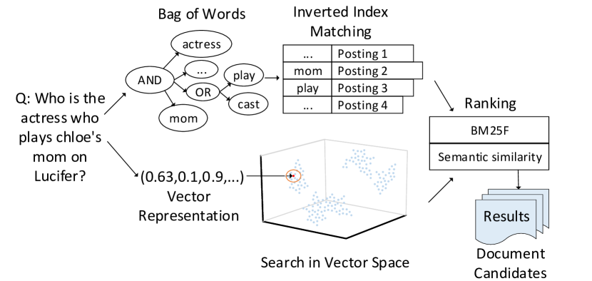
Figure 1: Example of traditional web search vs. semantic based vector search.

Searching for exact closest vectors is computationally expensive, especially when there are millions or even billions of vectors. In many cases, an approximate closest vector is almost as good as the exact one. Because of that, approximate nearest neighbor search (ANN) algorithms are often used for solving the high-dimensional vector search problem [3].

Real-world online services often pose stringent requirements on ANN search: high accuracy for effectiveness, low latency and small memory footprint for efficiency. High accuracy is clearly important because the approximation has to return true nearest neighbors with high probability (e.g., $>0.95$, or $>0.99)$; otherwise, users will not be able to find what they are looking for and the service is useless. Low latency is crucial because online systems often come with stringent service level agreement (SLA) that requires responses to be returned within a few or tens of milliseconds. Delayed responses could degrade user satisfaction and affect revenue [15]. Small memory footprint is another important factor because memory is a scarce machine resource — a memory efficient design is more scalable, e.g., reducing the number of machines needed to host billions of vectors, and empowering memory-constrained search on mobile devices and shared servers.

Popular existing approaches tackle ANN problems in high-dimensional space in two ways — graph-based and quantization-based, both of which face challenges to offer desired accuracy, latency and memory all together. The graph-based ANN approaches search nearest neighbors by exploring the proximity graph based on the closeness relation between nodes. They achieve high accuracy and are fast, but they yield high memory overhead as they need to maintain both the original vectors and additional graph structure in memory [34, 35]. Moreover, graph search requires many random accesses, which does not scale well on secondary storages such as SSDs. In a separate line of research, quantization-based ANN approaches, in particular product quantization (PQ) and its extensions, support low memory footprint index by compressing vectors into short code. They, however, suffer from accuracy degradation [22, 16, 25], as the approximated distances due to compression cannot always differentiate the vectors according to their true distances to queries.

In this paper, we tackle these challenges and propose an ANN solution, called Zoom, which collaboratively optimizes accuracy, latency and memory to offer both effectiveness and efficiency. In particular, we build Zoom based on a multi-view approach: a preview-step with quantized vectors in-memory, which quickly generates a small set of candidates that have a high probability of containing the true top-$K$ NNs, and a full-view step on SSDs to rerank those candidates with their full-length vectors. To improve efficiency, we design Zoom to reduce memory footprint through quantized representations and optimize latency through optimized routing and distance estimation; as for effectiveness, Zoom achieves high accuracy by reranking the close neighbors with full-length vectors to correctly identify the closest ones among them.

We evaluate Zoom on two popular datasets SIFT1M and Deep10M. We compare its effectiveness and efficiency with well-known ANN implementations including IVFPQ and HNSW. For efficiency, we not only measure classic metrics of latency and memory usage, we also propose and evaluate an ultimate efficiency/cost metric — VQ, i.e., VQ = number of Vectors per machine $\times$ Queries per second, inspired by DQ metric of web search engine [17]. For a given ANN workload with a total number of vectors $Y$ and total QPS of $Q$, an ANN solution requires $Y\times Q/VQ$ number of machines. The higher the VQ, the less machines and cost!

Our evaluation shows that, comparing with IVFPQ, Zoom obtains significantly higher accuracy (from about 0.58–0.68 to 0.90–0.99), while improving VQ by 1.7–8.0 times. To meet similar accuracy target, we improve VQ by 12.2–14.9 times, which is equivalent to saving 12.2–14.9 times of infrastructure cost. Comparing with HNSW, Zoom achieves 2.7–9.0 times VQ improvement with comparable accuracy. As online services like web search host billions of vectors and serve thousands of requests per second through vector search, a highly cost-efficient solution like Zoom could save thousands of machines and millions of infrastructure cost per year.

The main contributions of the paper are summarized as below:

• Identify important effectiveness and efficiency metrics (i.e., VQ) of ANN search to offer cost-efficient high-quality online services.

• Develop a novel ANN solution — Zoom— that strikes for the highest VQ and thus lowest infrastructure cost while obtaining desired latency, memory, and accuracy.

• Zoom is the first ANN index that intelligently leverages SSD to reduce memory consumption while attaining compatible latency and accuracy.

• Implement and evaluate Zoom: it collaboratively optimize latency, memory and accuracy, obtaining an order of magnitude improvements on VQ comparing with the state-of-the-art.

2 Background and Motivation

We first describe the vector search problem and then introduce the state-of-the-art ANN approaches. In particular, we describe NN proximity graph based approaches and quantization based approaches, which are two representative lines.

2.1 Vector Search and ANN

The vector search problem is formally defined as:

Definition 2.1.

Vector Search Problem. Let $Y=\{y_{1},...,y_{N}\}\in\mathds{R}^{D}$ represent a set of vectors in a $D$-dimensional space and $q\in\mathds{R}^{D}$ the query. Given a value $K$, vector search finds the $K$ closest vectors in $Y$ to $q$, according to a pair-wise distance function $d\langle q,y\rangle$, as defined below:

$$TopK_{q}=\underset{y\in Y}{\operatorname{K-argmin}}\ d\langle q,y\rangle$$ (1)

The result is a subset ${TopK_{q}}\subset Y$ such that (1) $|{TopK_{q}}|=K$ and (2) $\forall\ y\in Y-{TopK_{q}},and\ y_{q}\in TopK_{q}:d(q,y_{q})\leq d(q,y)$ [41].

In practice, the size $N$ of the set $Y$ is often large, so the computation cost of an exact solution is extremely high. To reduce the searching cost, approximate nearest neighbor (ANN) search is used, which returns the true nearest neighbors with high probability. Two lines of research have been conducted for high dimensional data: NN proximity graph based ANN and quantization based ANN, which are briefed below.

2.2 NN Proximity Graphs

The basic idea of NN proximity graph based methods is that a neighbor’s neighbor is also likely to be a neighbor [13]. It therefore relies on exploring the graph based on the closeness relation between a node and its neighbors and neighbors’ neighbors. Among those, the SWG (small world graph) approach builds an NN proximity graph with the small-world navigation property and obtains good accuracy and latency [34]. Such a graph is featured by short graph diameter and high local clustering coefficient. Yuri Malkov et al. introduced the most accomplished version of this algorithm, namely HNSW (Hierarchical Navigable Small World Graph), which is a multi-layer variant of SWG. Research shows that HNSW exhibits $O(\log N)$ search complexity ($N$ represents the number of nodes in the graph), and performs well in high dimensionality [34, 35, 27].

HNSW and other NN proximity graph based approaches store the full length vectors and the full graph structure in memory, which incurs a memory overhead of $O(N\times D)$. Such a requirement causes a high cost of memory.

2.3 Quantization-based ANN Search

Another popular line of research for ANN search in high-dimensional space involves compressing high-dimensional vectors into short codes using product quantization and its extensions [22, 16, 25].

2.3.1   Product quantization

Product quantization (PQ) takes high-dimensional vectors $y\in\mathds{R}^{D}$ as the input and splits them into $M$ subvectors: $y=[y^{1},...,y^{M}]$, where each $y^{m}\in\mathds{R}^{D^{\prime}},D^{\prime}=D/M$. Then these subvectors are quantized by $M$ distinct vector quantizers as: $pq(y)=[vq^{1}(y^{1}),...,vq^{M}(y^{M})]$. Each vector quantizer $vq^{m}$ has its own codebook, denoted by $C^{m}\subset\mathds{R}^{D^{\prime}}$, which is a collection of $L$ representative codewords $C^{m}=\{c^{m}_{1},...,c^{m}_{L}\}$. The codebook $C^{m}$ can be built using Lloyd’s algorithm [32]. The vector quantizer $vq^{m}$ maps each $y^{m}$ to its closest codeword in the codebook:

$$y^{m}\mapsto vq^{m}(y^{m})=\underset{c^{m}_{i}\in C^{m}}{\operatorname{argmin}}\ d\langle y^{m},c^{m}_{i}\rangle.$$ (2)

The codebook of the product quantizer is the Cartesian product of the $M$ codebooks of those vector quantizers:

$$C_{pq}=C^{1}\times...\times C^{M}$$ (3)

This method therefore could create $L^{M}$ codewords, but it only requires to store $L\times M\times D$ values for all its codebooks.

In practice, PQ maps the $m$-th subvecter of an input vector $y$ to an integer $(1,...,L)$, which is the index to the codebook $C^{m}$, and concatenates resultant $M$ integers to generate a PQ code of $y$. The memory cost of storing the PQ code of each vector is $B=M\ \times log_{2}{(L)}$ bits. Typically, $L$ is set to 256 so that each subvector index is represented by one byte, and $M$ is set to divide $D$ evenly.

2.3.2   Two-level quantization

PQ and its extensions reduce the memory usage per vector. However, the search is still exhaustive in the sense that the query is compared to all vectors. For large datasets, even reading highly quantized vectors is a severe performance bottleneck due to limited memory bandwidth. This leads to a two-level approach: at the first level, vectors are partitioned into $N_{cluster}$ clusters, represented by a set of cluster centroids $S_{centroid}=\{c_{1},...,c_{N_{cluster}}\}$. Each $y$ then is mapped to its nearest cluster centroid through a mapping function $f_{cluster}$:

$$y\mapsto c_{y}=\underset{c_{i}\in C_{cluster}}{\operatorname{argmin}}\ d\langle y,c_{i}\rangle.$$ (4)

The set of of vectors $V_{i}$ mapped to the same cluster is therefore defined as:

$$V_{i}=\{y\in\mathds{R}^{D}:f_{cluster}(y)=c_{i}\}.$$ (5)

At the second level, the approach uses a product quantizer $q_{pq}:\mathds{R}^{D}\mapsto C_{pq}\subset\mathds{R}^{D}$ to quantize the residual vector, defined as the difference between $y$ and its mapped cluster centroid $c_{i}$. A database vector $y$ is therefore approximated as

$$y\approx f_{cluster}(y)+q_{pq}(y-f_{cluster}(y))$$ (6)

Together we refer this two-level scheme as IVFPQ  [22]. While processing a query, IVFPQ enables non-exhaustive searches, by finding either the closest or several of the closest clusters and scanning associated vectors only in those selected clusters at the second level [22].

3 Challenges

Both graph-based and quantization-based prior work faces challenges to offer desired accuracy, latency, and memory all together.

Challenge I. Graph-based approaches are efficient, but they are memory consuming and do not scale well to SSDs.

While graph-based approaches attain good latency and accuracy, their indices are memory consuming in order to store both full-length vectors and the additional graph structure  [35]. As the number of vectors grows, its scalability is limited by the physical memory of the machine, and it becomes much harder to host all vectors on one machine. A distributed approach would suffer from poor load balancing because the intrinsic nature of power-law distribution of queries [39], making scale-out inefficient. On the other hand, SSDs have been widely used as secondary storage, and they are up to 8X cheaper and consume less than ten times power per bit than DRAM [43, 31, 36]. Many search engines such as Google and Bing already have SSDs to store the inverted index due to the factors such as cost, scalability, and energy [44, 37, 44, 45]. However, it is difficult to make HNSW work effectively on SSDs because the search of the graph structure generates many non-contiguous memory accesses, which are much slower on SSDs than memory and detrimental to the query latency.

Challenge II. Quantization helps memory saving but results in poor recall.

The recall metric measures the fraction of the top-$K$ nearest neighbors retrieved by the ANN search which are exact nearest neighbors.

Quantization-based approaches, including IVFPQ, suffer from low recall. As a point of reference, with 64 times compression ratio, both IVFPQ and its most advanced extension LOPQ achieve $<0.4$ recall when $K=1$  [22, 25].

To see the reason behind why IVFPQ and in general quantization-based approaches incur low recall, especially with large compression ratio, let us see a simple example as illustrated in Fig. 2.

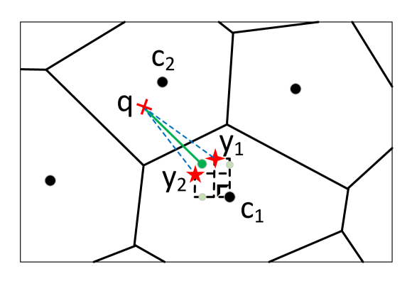
Figure 2: 2D IVFPQ example of the lossy procedure of quantization-based approaches. $q$ denotes the query, $y_{1}$ and $y_{2}$ (drawn as a red cross) denotes vectors. $c_{1}$ and $c_{2}$ represent cluster centroids.

Assume we have a 2D vector space with two vectors $y_{1}$ and $y_{2}$ assigned to the same first-level cluster represented by $c_{1}$. Because the quantization process is lossy, $y_{1}$ and $y_{2}$ might be quantized to have the same PQ code (represented by the green dot). Their distance to a query $q$ is the same, and it is impossible to differentiate which one is closer to the query using the quantized vectors. As a result, quantization generate non-negligible recall loss.

Challenge III. Quantization-based approaches face a dilemma on optimizing latency.

As one-level quantization suffers from exhaustive scan, we focus on two-level quantization, whose latency is decomposed into two parts: the cluster selection time ($T_{CS}$) and the vector scanning time ($T_{VS}$) in selected clusters. Both latency components depend on the number of the first-level clusters $N_{cluster}$. During cluster selection, an exhaustive search is used to find out a few clusters closest to the query to scan, and $T_{CS}$ in this case is linear in $N_{cluster}$. When $N_{cluster}$ is not too large, finding which cluster to scan is computationally inexpensive. Existing approaches rarely choose a large $N_{cluster}$, because as $N_{cluster}$ increases, $T_{CS}$ itself would become too long, prolonging query latency. Fig. 3 shows that for 1M vectors with $N_{cluster}$ $=16K$, $T_{CS}$ already takes a significant portion of execution time than $T_{VS}$.

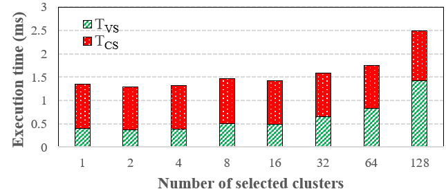
Figure 3: SIFT1M dataset: Evaluation of cluster selection time $T_{CS}$ and vector scanning time $T_{VS}$ with two-level quantization-based approach. The x-axis represents the number of selected clusters out of a total of 16K clusters.

On the other end, larger $N_{cluster}$ leads to a smaller percentage of vectors to be scanned at the second level to reach the same recall. Fig. 4a shows that given three different values of $N_{cluster}$ 1K, 4K, and 16K, scanning the same number of clusters (e.g., 64) all lead to close or very similar recall. This observation is kind of intuitive as top $K$ NNs would belong to at most $K$ clusters regardless of $N_{cluster}$ value. As larger $N_{cluster}$ has less (expected) number of vectors per cluster, this observation indicates that larger $N_{cluster}$ requires less number of vectors to be scanned at the second level. Figure 4b confirms that by scanning 64 clusters, only 0.4% cells need to be scanned when $N_{cluster}$ is $16K$ whereas it is 6.4% when $N_{cluster}=1K$, which means the search at the second level can take much longer time with smaller $N_{cluster}$.

The $N_{cluster}~{}$ dilemma makes it challenging to optimize both $T_{CS}$ and $T_{VS}$. The problem is beyond selecting a good value for $N_{cluster}$ ; it requires more fundamental change on ANN design for latency optimization.

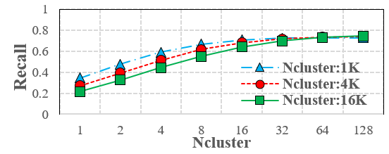
(a) Evaluation of recall of two-level quantization. All three configurations can reach almost the same recall by scanning the same number of clusters.

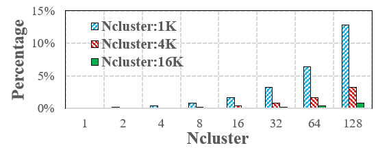
(b) Plot of the percentage of selected clusters to scan. Given the same number of clusters to select, larger $N_{cluster}$ requires a smaller percentage of clusters to be scanned.

Figure 4: SIFT1M dataset: Evaluation of recall and the percentage of scanned clusters with two-level quantization for three different number of clusters $N_{cluster}$. The x-axis is the number of selected clusters to scan.

4 Design Overview

In this section, we propose an ANN search solution to address the aforementioned challenges, offering low latency, high memory efficiency, and high recall all together. The software architecture overview is presented in Fig. 6.

First, a key empirical observation enlightened us to solve the poor recall challenge of quantization such that we can achieve high memory efficiency and high recall together — Although the approximated top-$K$ NNs might not always match the exact top-$K$ NNs due to the precision loss from quantization, the approximated top-$K$ NNs are more likely to fall within a list of top-$R$ candidates, where $R$ is larger but not too much larger than $K$.

Observation on quantization recall.

We made the observation through recall analysis of IVFPQ, and we found it general towards various datasets (more results in Section 7.2). Fig. 5a shows an example on SIFT1M dataset, where we apply IVFPQ by partitioning the vector space into $16K$ clusters and quantizes vectors with a compression ratio of 16X. By scanning 512 clusters ( 3% of the total clusters), the likelihood of finding the top-1 NN in top-10 candidates is 99.7%, whereas the probability of an exact match is only 71.8%. Similarly, Fig. 5b shows that the probability of finding the top-10 NNs in top-50 candidates is close to 1, whereas the recall (e.g., when R=10) is only 78.9%. This is presumably because quantization makes it impossible to differentiate true NNs from their neighbor vectors if they are quantized to have the same PQ code, as shown in Fig. 2 in Section 3. Therefore, the true NNs are included in top-$R$ but cannot be identified due to the precision loss. Our analysis indicates that such relation holds for $K>1$ as well.

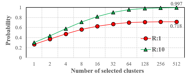
(a) Probabilties of top-1 NN falls within top-R candidate results. Although the approximated top-1 might not always match the exact top-1 NN, the top-1 NN has a high chance to be within the top-10 results.

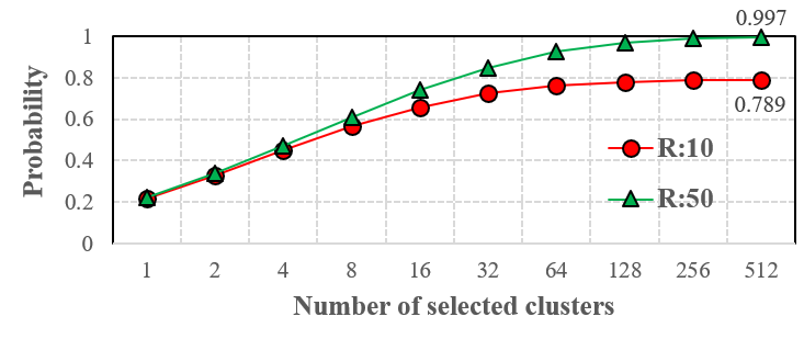
(b) Probabilties of top-10 NNs fall within top-R candidate results. The approximated top-10 results are more likely to be within the top-50 candidates.

Figure 5: A key observation from quantization recall analysis.

Overview.

Based on the observation, we propose an ANN design, called Zoom, that employs a "multi-view" approach as an accuracy enhancement procedure, contrasting it with a single-view approach (either quantized representation, as in IVFPQ, or full-length vectors, as in HNSW). The multi-view approach contains two steps:

• A preview step in memory that employs a preview index as a filter to generate a small candidate set of top-$R$ NNs based on quantized vectors;

• A full-view step on SSDs that reranks the selected NNs from the preview step based on their full-length vectors and selects top-$K$ NNs from the top-$R$ candidates.

Intuitively, such a multi-view design achieves memory savings, through in-memory preview on quantized data, and high recall, through SSD-based reranking on full-length vectors, but what about latency? The full-view step only needs to rerank a small set of candidates, so this part of latency is less of a big concern, but what about the preview step? To address the latency challenge of quantization, the preview step of Zoom is powered by a cluster routing layer (CRL) together with a product quantization layer (PQL). The cluster routing layer leverages HNSW to quickly and accurately dispatch a query to a few nearest clusters, instead of scanning centroids of all clusters. HNSW reduces the cluster selection cost from $O(N_{cluster})$ to $O(\log(N_{cluster}))$, and thus, Zoom can choose a relatively large value of $N_{cluster}$ with affordable $T_{CS}$ and small $T_{VS}$, addressing Challenge III and optimizing latency. The product quantization layer compresses vectors through product quantization with optimized distance computation that improves overall system efficiency.

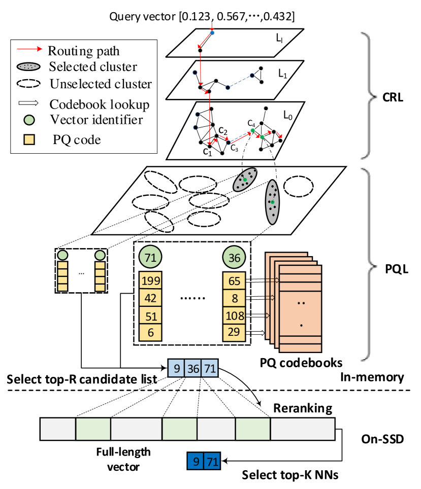
Figure 6: The Zoom architecture.

Next, we describe Zoom index construction in Section 5 and query processing in Section 6.

5 Index Construction

Given a set of vectors, Zoom builds the in-memory preview index using Algorithm 1, with 3 major steps:

• Clustering. Cluster on the set of data vectors $Y$ to divide the space into $N_{cluster}$ clusters. Zoom keeps the set of centroids of those clusters at $S_{centroid}$ (line 4).

• Routing layer construction. Use HNSW to build a routing structure on top of $S_{centroid}$ to quickly identify a few closest clusters to scan (line 5). Perform connectivity augmentation to ensure the reachability of clusters (line 6).

• PQ layer generation. The PQ layer leverages product quantization to generate PQ codebooks and PQ encoded vectors [22]. To generate PQ codebooks, Zoom first calculates the residual distance of each vector to the cluster it belongs to (line 7–line 10). It then splits the vector space into $M$ sub-dimensional spaces and constructs a separate codebook for each sub-dimension (line 11–line 13). Thus, Zoom has $D/M$ dimensional codebooks for $M$ sub-dimension, each with $L$ subspace codewords. Generating the codebooks based on residual vectors is a common technique to reduce the quantization error [24, 22]. Zoom then generates PQ encoded vectors by assigning the PQ code for each vector (i.e., a concatenation of $M$ indices) and adds each quantized vector to the cluster it belongs to (line 15–line 18). Furthermore, Zoom precomputes terms used for the PQ code distance computation and store the precomputed results into a cache (line 19–line 20). Such a precomputation helps reduce memory accesses during the search phase to obtain lower latency.

Full-view index. Zoom stores and uses full-length vectors for reranking. It keeps vectors as binary vectors byte-aligned as a file on SSDs (line 21), which allows each vector to be selected through random access (e.g., based on vector id/offset). Using HDDs is detrimental to query latency because the slow, mechanical sector seek time for random accesses.

Algorithm 1 Zoom index construction algorithm

1:Input: Vector set $Y$, vector dimension $D$.

2:Output: Zoom index.

3:Parameter: Number of sub-dimensional spaces $M$, number of sub-codewords $L$ in each sub-codebook, size of clusters $N_{cluster}$.

4:$index.S_{centroid}\leftarrow clustering(Y,D,N_{cluster})$ $\triangleright$ Partition the vector space using K-Means algorithm.

5:$index.routing\_layer\leftarrow CreateHnsw(S_{centroid},M)$

6:$connectivity\_augmentation(routing\_layer)$

7:for all $i$ in 0..($N-1$) do

8:     $cell\_id,codeword\leftarrow assign(Y[i],S_{centroid})$

9:     $R[i]\leftarrow compute\_residual(Y[i],codeword)$

10:     $CID[i]\leftarrow cell\_id$

11:for all $i$ in 0..($M-1$) do

12:     $codebook\leftarrow train\_residual(R[:i\times D/M,(i+1)\times D/M],L))$

13:     $pq\_codebook.set(i,codebook)$

14:$index.pq\_layer.add(pq\_codebook)$

15:for all $i$ in 0..($N-1$) do

16:     $cell\_id\leftarrow CID[i]$

17:     $Y_{pq\_code}[i]\leftarrow product\_quantizer(R[i])$

18:     $pq\_layer.lists[cell\_id].add(Y_{pq\_code}[i])$

19:for all $i$ in 0..($N-1$) do

20:     $index.cache[i]\leftarrow precompute\_term(R[i],CID[i])$

21:$store\_fullview\_vectors()$

5.1 Routing Layer Construction

Performing exact search to find the closest clusters incurs complexity of $O(N_{cluster}\times D)$. We explore HNSW as a routing scheme to perform approximate search, achieving $O(\log(N_{cluster})\times D)$ complexity while attaining close to unity recall with fast lookup [34, 35, 27].

HNSW index for routing

We describe the main ideas and refer readers to  [35] for more details. The routing layer is built incrementally by iteratively inserting each centroid $c_{i}$ of $S_{centroid}$ as a node. Each node generates $OutD$ (i.e., the neighbor degree) out-going edges. Among these, $OutD-1$ are short–range edges, which connect $c_{i}$ to $OutD-1$ closest centroids according to their pair-wise Euclidean distance to $c_{i}$ (e.g., the edge between $c_{1}$ and $c_{2}$ in Fig. 6). The rest is a long–range edge that connects $c_{i}$ to a randomly picked node, which does not necessarily connect two closest nodes but may connect other locally connected node clusters (e.g., the edge between $c_{3}$ and $c_{4}$ in Fig. 6). It is theoretically justified that constructing a proximity graph by inserting these two types of edges offers the graph small-world properties [46, 34, 35].

The constructed small world graph using all $c_{i}$ becomes the ground layer $L_{0}$ of CRL. Zoom then creates a hierarchical small world graph by creating a chain of subsets $V=L_{0}\supseteq L_{1}\supseteq\ldots\supseteq L_{l}$ of nodes as "layers", where each node in $L_{i}$ is randomly selected to be in $L_{i+1}$ with a fixed probability $1/OutD$. On each layer, the edges are defined so that the overall structure becomes a small world graph, and the number of layers is bounded by $O\left(\log(N_{cluster})/\log(OutD)\right)$ [34].

Connectivity augmentation.

HNSW does not guarantee the reachability of all nodes. There can be a large amount of "isolated nodes" at the ground layer, which are nodes with zero in-degree. When used as a routing scheme, it is crucial to ensure reachability as an entire cluster will be missed if HNSW cannot reach its centroid. Fig. 7 shows the frequency distributions of in-degree for all nodes in the routing layer . Without optimization (Fig. 7 (top)), there are around 1,000 nodes whose in-degree are zero. These nodes and their corresponding clusters cannot be reached during the search process.

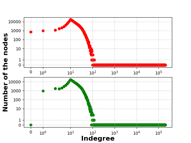
Figure 7: Indegree histogram of the HNSW routing layer.

We develop a new technique called connectivity augmentation to resolve the issue. We apply Kosaraju’s algorithm [18] against the constructed routing layer. This step (line 6) adjusts the routing layer by adding minimal number of edges to make the graph strongly connected without destroying its small world properties. Fig. 7 (bottom) shows that after connectivity augmentation, there are no zero in-degree nodes.

5.2 Towards Larger $N_{cluster}$

As shown in Fig. 4, the number of vectors to be scanned for a target accuracy is strongly determined by $N_{cluster}$. Choosing a large $N_{cluster}$ reduces that, so does the cluster scanning time.

A major challenge of having a large $N_{cluster}$ is the cluster selection time $T_{CS}$, which we address through the HNSW based routing. Another challenge is that the standard K-Means algorithm is prohibitively slow. To boost the speed of clustering with large $N_{cluster}$, we employ Yingyang $K$-Means and GPU to perform the clustering, which speedup normal $K$-Means by avoiding redundant distance computation if cluster centroids do not change drastically in between iterations [12] . One nice property of this approach is that it serves as a drop-in replacement and yields exactly the same results that would be achieved by ordinary $K$-Means.

Memory consumption is another concern, yet even a large $N_{cluster}$ is still relatively small compared to the quantized representation of the entire set of vectors. The memory cost of Zoom index is given by:

$$\begin{split}MO&=N\times(M\times\frac{log(L)}{8\textnormal{-}bit}+f)+L\times D\times f\\ &+N_{cluster}\times(D+OutD)\times f\ ,\end{split}$$ (7)

which is the sum of the size of cluster centroids ($N_{cluster}\times D\times f$), metadata for the routing layer ($N_{cluster}\times 2\times OutD\times f$), the PQ codebooks ($L\times D\times f$ bytes), and the PQ code ($M\times\frac{log(L)}{8\textnormal{-}bit}$) plus $f$-byte per vector for caching the precomputation result, where $f$ denotes the number of bytes of vector data type.

6 Query Processing

We describe how Zoom searches top-$K$ NNs. Algorithm 2 shows the online search process. Preview search happens in memory, starting from the routing layer, which returns the ids ($I^{Nscan}$) and distance ($D^{Nscan}$) of $Nscan$ selected clusters (line 4). For those selected clusters, Zoom scans vectors in each of them at the PQ layer and keeps track of the top-$R$ closest candidate NNs (line 5). The top-$R$ candidates are reranked during full view (line 6).

Algorithm 2 Zoom online search algorithm

1:Input: Query vector $q$, number of nearest neighbors $K$ to retrieve.

2:Output: Top-$K$ nearest neighbors.

3:Parameter: number of clusters to scan $Nscan$, size of HNSW search queue $efSearch$, size of candidate list $R$.

4:$I^{Nscan},D^{Nscan}\leftarrow index.routing\_layer.search(q,Nscan)$ $\triangleright$ Return top-$Nscan$ clusters with minimal distance to $q$.

5:$TopR\leftarrow scan\_pq\_vectors(q,I^{Nscan},D^{Nscan})$ $\triangleright$ Preview step.

6:$TopK\leftarrow rerank\_with\_fullview\_vectors(q,TopR)$ $\triangleright$ Full-view step.

6.1 Preview Step

Clusters selection. Zoom selects clusters using the search method from HNSW [35], which is briefly described below. The search starts from the top of the routing layer and uses greedy search to find the node with the closest distance to the query $q$ as an entry point to descend to the lower layers. The upper layers route $q$ to an entry point in the ground layer that is in a region close to the nearest neighbors to $q$. Once reaching the ground layer, Zoom employs prioritized breath-first search: It exams its neighbors and stores all the visited nodes in a priority queue based on their distances to the $q$. The length of the queue is bounded by $efSearch$, a system parameter that controls the trade-off between search time and accuracy. When the search reaches a termination condition (e.g., the number of distance calculation), Zoom returns $Nscan$ closest clusters.

PQ layer distance computation.

Zoom calculates the distance from query $q$ to a data point $y$ in cluster $V_{i}$ using its PQ code and asymmetric distance computation (ADC) [22]:

$$d\langle q,y\rangle\!\!\! = \!\!\!\!d\langle q-c,r\rangle\sim d_{ADC}\langle q-c,pq(r)\rangle$$ (8)

$$= \!\!\!\!\sum_{m=1}^{M}{d\langle(q-c)^{m},vq^{m}(r^{m})\rangle}$$ (9)

where $c$ is the cluster center and $r$ is the residual distance between $y$ and $c$, represented as $[r^{1}:,,,:r^{M}]$. It can be expanded into four terms for Euclidean norm calculation [4]:

$$\underset{Term-A}{\underline{\|x-c\|^{2}}}+\underset{Term-B}{\underline{\sum_{m=1}^{M}{\|c_{y^{m}}^{m}\|}^{2}}}+\underset{Term-C}{\underline{2\sum_{m=1}^{M}{\langle c^{m},c_{y^{m}}^{m}\rangle}}}-\underset{Term-D}{\underline{2\sum_{m=1}^{M}{\langle x^{m},c_{y^{m}}^{m}\rangle}}}$$ (10)

where $c_{y^{m}}^{m}=vq^{m}(r^{m})$, denoting the closest sub-codeword assigned to sub-vector $y^{m}$ in the $m$-th sub-dimension.

Existing approach calculates these terms on-the-fly for each query by calculating them and reusing the results with look-up tables (LUTs). Without optimization, it requires $2\times M$ lookup-add operations to estimate the distance per data point.

By looking close into these terms, we notice that each term can be query dependent (query-dep.), mapped centroid dependent (centroid-dep.), and/or PQ code dependent (PQ-code-dep.). Table 1 summaries these dependencies.

	Query-dep.	Centroid-dep.	PQ-code-dep.
Term-A	✓	✓	✗
Term-B	✗	✗	✓
Term-C	✗	✓	✓
Term-D	✓	✗	✓

Table 1: Dependencies of PQ distance computation.

Since both Term-B and Term-C are query independent, Zoom precomputes Term-B and Term-C and caches their sum for each data point as a post-training step. During query processing, it takes a single lookup to get the sum of Term-B and Term-C. It then requires only $M+1$ lookup-add operations to estimate the distance, with the trade-off of adding $f$-byte memory (e.g., 4-byte if vector type is float) per data point. The $scan\_pq\_vectors()$ method in Lst. 1 shows how Zoom scans a cluster with the optimized distance computation.

Listing 1: Method to scan PQ vectors

⬇

1scan_pq_vectors(q, $I^{Nscan}$, $D^{Nscan}$)

2 TopR = min_priority_queue()

3 // init LUTs for computing all possible Term-D

4 for m in M:

5 for l in L:

6 termD_LUT[m][l] = -2 x $\langle x^{m},c_{l}^{m}\rangle$

7 for n in 0..($Nscan-1$):

8 cluster = index.pq_layer.list$[I^{Nscan}[n]]$

9 // Compute Term-A

10 t1 = $\|q-D^{Nscan}[n]\|^{2}$

11 for v in cluster:

12 // M lookup-add Term-D

13 for m in M:

14 dist += termD_LUT[m]

15 // Lookup-add precomputed Term-B and Term-C in the index construction phase

16 dist += index.cache[v]

17 TopR.push(v, dist)

18 return TopR

6.2 Full-view Step

Zoom employs existing optimization techniques to reduce SSD access latency of reranking top-$R$ candidate NNs.

i) Batched, non-blocking multi-candidate reranking.

Synchronous IO is slow due to its round trip delay. Zoom leverage asynchronous batching by combining $B$ candidate vectors in the candidate list into one big batch and submit $S=\lceil R/B\rceil$ asynchronous batched requests to SSD. Batched requests allow Zoom to exploit the internal parallelism of SSD. Asynchronous IO avoids blocking Zoom search and allows it to recompute a vector as soon as its full-view vector has been loaded into memory. Zoom uses auto-tuning to identify the optimal combination of $B$ and $S$.

ii) OS buffered I/O bypass.

Zoom employs direct IO to bypass the system page cache to suppress the memory interference caused by loading full-view vectors stored on SSD. Modern operating systems often maintain page cache, where the OS kernel stores page-sized chunks of files first into unused areas of memory, which acts as a cache. In most cases, the introduction of page cache could achieve better performance. However, there are two main reasons we want Zoom to opt-out of system page cache: 1) the reranking of candidates mostly incur random reads, which increases cache competition with a poor cache reuse characteristics; 2) page caching fullview vectors increases the memory cost to host Zoom index, decreasing its memory efficiency.

Implementation.

We implement the SSD-based reranking using the Linux NVMe Driver. The implementation uses the Linux kernel asynchronous IO (AIO) syscall interface, io_submit, to submit IO requests and io_getevents to fetch completions of loaded full-length vectors on SSD. Batched requests are submitted through an array of iocb struct at one. We open the file that stores the full-length vectors in O_DIRECT mode to bypass kernel page cache. Apart from Linux, most modern operating systems, including Windows, allow application to issue asynchronous, batched, and direct IO requests [1, 2]. There are also other advanced NVMe drivers like SPDK [21] and NVMeDirect [26], which offers even better performance on SSD by moving drivers into userspace and enable optimizations such as zero-copy accesses. We choose AIO for its simplicity and compatibility.

7 Evaluation

We evaluate Zoom and show how its design and algorithms contribute to its goals.

7.1 Methodology

Workload.

We use SIFT1M and Deep10M datasets for the experiments.

• SIFT1M [22] is a classical dataset to evaluate nearest neighbor search [33]. It consists of one million 128-dimensional SIFT vectors, where each vector takes 512-byte to store .

• Deep10M is a dataset that consists of 10 millions of 96-dimensional feature vectors generated by deep neural network [5] . Each vector requires 384-byte memory.

	$N_{scan}$	IVFPQ						Zoom
		Recall	Lat.	Mem.	Recall	Lat.	Mem.	Recall	Lat.	Mem.	VQ im.	Recall	Lat.	Mem.	VQ im.
		$\approx$32 bytes per vector			$\approx$64 bytes per vector			$\approx$36 bytes per vector				$\approx$68 bytes per vector
SIFT1M	1024	0.679	8.8	40	0.850	10.3	71	0.894	0.5	49	12.3X	0.898	0.9	80	12.2X
								$(N_{scan}:32)$				$(N_{scan}:32)$
	512	0.678	5.4	40	0.849	6.1	71	0.989	1.8	49	2.5X	0.999	3.1	80	1.7X
	256	0.676	3.2	40	0.847	3.9	71	0.986	1.2	49	2.2X	0.995	1.8	80	1.9X
	128	0.672	2.5	40	0.840	2.7	71	0.976	0.8	49	2.4X	0.984	1.3	80	1.8X
	64	0.662	2.0	40	0.820	2.0	71	0.948	0.7	49	2.4X	0.955	0.9	80	1.9X
		$\approx$24 bytes per vector			$\approx$48 bytes per vector			$\approx$28 bytes per vector				$\approx$52 bytes per vector
Deep10M	1024	0.602	18.5	302	0.866	24.6	531	0.906	0.8	377	12.6X	0.921	1.4	606	14.9X
								$(N_{scan}:64)$				$(N_{scan}:64)$
	512	0.601	15.6	302	0.863	18.9	531	0.975	5.4	377	2.3X	0.994	4.6	606	3.6X
	256	0.599	14.1	302	0.856	15.7	531	0.965	3.4	377	3.3X	0.982	2.8	606	4.9X
	128	0.594	13.1	302	0.843	14.2	531	0.946	2.4	377	4.3X	0.963	1.9	606	6.4X
	64	0.580	12.8	302	0.812	13.1	531	0.906	2.0	377	5.2X	0.921	1.4	606	8.0X

Table 2: Recall, latency (ms), memory (MB), VQ improvement of Zoom in comparison with IVFPQ given different compression ratio and $N_{scan}$ for two datasets.

Evaluation metrics.

Latency, memory cost, and recall are important metrics for ANNs. We measure query latency as the average elapsed time of per-query execution time in millisecond. The memory cost is calculated as the total allocated DRAM for the ANN index. The recall of top-$K$ NNs is calculated as $\frac{|\xi(q)\bigcap\theta(q)|}{K}$, where $\xi(\cdot)$ and $\theta(\cdot)$ denote the set of exact NNs and the NNs given by the algorithm.

In this paper, we also employ VQ (Vector–Query) as an important cost metric for ANN, inspired by the DQ (Document–Query) metric from web search engine [17]. VQ is defined as the product of the number of vectors per machine and the queries per second. For a given ANN workload with a total number of vectors $Y$ and total QPS of $Q$, an ANN solution requires $Y\times Q/VQ$ number of machines. The higher the VQ, the less machines and cost! VQ improvement over baseline ANNs is calculated as a product of the latency speedup and memory cost reduction rate.

Implementation.

Zoom is implemented in C++ on Faiss , an open source library for approximate nearest neighbor search. The routing layer is implemented based on a C++ HNSW implementation from the HNSW authors . By default, Faiss evaluates latency with a very large batch size (10000) and report the execution time as the total execution time divided by the batch size. Such a configuration does not represent online serving scenarios, where requests often arrive one-by-one. We choose query batch size of 1 to represent a common case in online serving scenario. When batch size is small, Faiss has other performance limiting factors, e.g., unnecessary concurrency synchronization overhead, which we address in Zoom. Also, neither Faiss nor HNSW parallelizes the execution of single query request. To make results consistent and comparable, Zoom does the same.

Experiment platform.

We conduct the experiments on Intel Xeon Gold 6152 CPU (2.10GHz) with 64GB of memory and 1TB Samsung 960 Pro SSD. The server has one GPU (Nvidia GeForce GTX TITAN X) which is used for clustering during index construction.

7.2 ANN Search Performance Comparison

We first measure the performance results of Zoom and compare it with state-of-the-art ANN approaches: IVFPQ  and HNSW . Then we conduct a more detailed evaluation on the effect of different Zoom techniques.

7.2.1   Comparison to IVFPQ

	HNSW				Zoom				VQ
	Recall	efSearch	Latency	Memory	Recall	$N_{scan}$	Latency	Memory	Improvement
SIFT1M	0.993	1280	2.3	588	0.991	1024	3.1	49	9.0X
	0.984	640	1.2	588	0.989	512	1.8	49	8.2X
	0.973	320	0.6	588	0.976	128	0.8	49	8.6X
	0.947	160	0.3	588	0.948	64	0.7	49	5.3X
Deep10M	0.998	1280	3.1	4662	0.998	1024	6.7	377	5.8X
	0.993	640	1.6	4662	0.994	512	3.9	377	5.0X
	0.985	320	0.9	4662	0.983	256	2.6	377	4.2X
	0.969	160	0.4	4662	0.961	128	2.0	377	2.7X

Table 3: Latency (ms), memory (MB), and VQ improvement of Zoom in comparison with HNSW under comparable recall target.

Table 2 reports the recall (for $K=1$), latency, memory cost, and VQ improvement of Zoom, in comparison to IVFPQ, for two datasets. Both IVFPQ and Zoom partition the input vectors into $N_{cluster}$ clusters (20K for SIFT1M, and 200K for Deep10M ) and generate the same PQ codebooks to encode all vectors. We vary the selected clusters $N_{scan}$ from 64 to 1024. This is the range we start to see that further increasing $N_{scan}$ leads to diminishing return of recall from IVFPQ. We also vary memory requirement by quantizing vectors with two different compression ratios (16X and 8X): $\approx$32, 64 bytes per vector for SIFT1M, and $\approx$24, 48 bytes per vector for Deep10M, by choosing different $M$. Two main observations are in order.

First, the results show that Zoom provides significant improvement to the recall from about 0.58–0.68 to 0.90–0.99, while at the same time improving VQ by 1.7–8.0 times among tested configurations. As expected, by varying $N_{scan}$ from 64 to 512, the recall and latency increase for both implementations as scanning more clusters increases both the likelihood and time of finding top-$K$ NNs. The recall of IVFPQ is constantly lower than Zoom, and it starts to saturate at $N_{scan}=128$. In contrast, Zoom improves the recall by a large percentage. More importantly, it significantly improves the system’s effectiveness by bringing the recall to the $0.90+$ range. This is contributed by Zoom’s multi-view accuracy enhancement procedure. In terms of efficiency, Zoom overall speedups query latency in the range of 1.9–9.1 times, compared to IVFPQ, with a slightly higher memory cost due to the additional memory cost of storing the routing layer and caching precomputation results. The VQ im. column captures the VQ improvement where Zoom consistently outperforms IVFPQ.

Second, Zoom improves VQ by 12.2–14.9 times to meet similar or higher recall target. The highest recall IVFPQ can get is still far below 1 (e.g., at 0.679 when $N_{scan}=1024$ for SIFT1M). This is not because IVFPQ fails to scan clusters that include true NNs, but because some true NNs cannot be differentiated by their PQ code based distance to the query even when they get scanned. In contrast, Zoom does not suffer as much from this issue and can achieve similar or higher recall by scanning a much smaller number of clusters (e.g., 32 and 64 clusters as marked by the parentheses below the recall measure), which also leads to a lower latency.

7.2.2   Comparison to HNSW

We also compare Zoom with HNSW, the state-of-the-art NN proximity graph based approach. Since these two are very different solutions, we compare them by choosing configurations from both that achieve comparable recall targets (e.g., 0.95, 0.96, 0.97, 0.98, and 0.99) .

As reported by Table 3, Zoom significantly and consistently outperforms HNSW, with an average VQ improvement of 3.5–9.0 times among tested configurations. Zoom reduces the memory cost by around 12 times compared to HNSW. Although HNSW runs faster than Zoom in most cases, the latency gap between Zoom and HNSW decreases as we increase the recall target. This is presumably because for HNSW, further increasing $efSearch$ leads to little extra recall improvement but significantly more node exploration and distance computation when the recall is getting close to 1.

7.3 Effect of Different Components

Next, we conduct an in-depth evaluation across different design points of Zoom.

7.3.1   Latency of preview query processing

Fig. 8 shows the breakdown of query latency on searching the in-memory preview index.

Latency of the routing layer.

Our results show that HNSW based routing yields significant improvements on cluster selection time compared with the exact search in IVFPQ for both SIFT1M (Fig. LABEL:fig:in-memory-time-sift1m-cs) and Deep10M (Fig. LABEL:fig:in-memory-time-deep10m-cs). Overall, the HNSW routing layer speedups the cluster selection time by 3–6 times for SIFT1M ($N_{cluster}=20K$) and 10–22 times for Deep10M ($N_{cluster}=200K$). The HNSW routing layer offers higher speedup when the number of clusters $N_{cluster}$ is larger because the complexity of exact search is $O(D\times N_{cluster})$, whereas the complexity of HNSW based routing is $O(D\times\log{N_{cluster}})$, which is logarithmic to $N_{cluster}$. Therefore, the HNSW routing layer scales better as $N_{cluster}$ increases and the improvement becomes more significant with larger $N_{cluster}$ sizes.

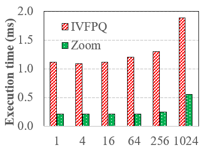
(a)

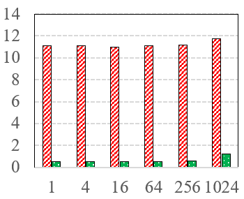
(b)

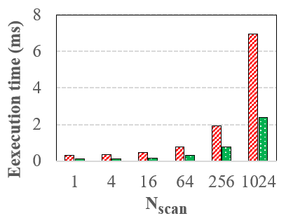
(c)

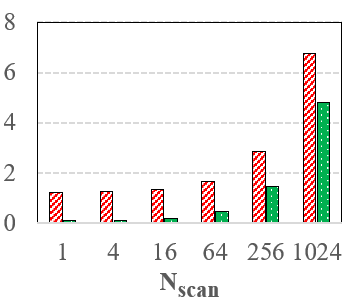
(d)

Figure 8: Effect of different components on the in-memory search query latency. The x-axis represents the number of selected and scanned clusters $N_{scan}$.

Latency of PQ layer.

Fig. LABEL:fig:in-memory-time-sift1m-vs and Fig. LABEL:fig:in-memory-time-deep10m-vs illustrate the improvements of query latency of the PQ layer compared to IVFPQ. As $N_{scan}$ increases, the execution time of the PQ layer increases almost linearly for both IVFPQ and Zoom. However, the PQ layer in Zoom consistently outperforms IVFPQ by 2–13 times. This is because Zoom optimizes the distance computation by reducing $2\times M$ lookup-add operations to $M+1$ lookup-add per vector, significantly reducing memory accesses and mitigating memory bandwidth consumption.

7.3.2   Accuracy of HNSW-based routing

Here we evaluate how accurately HNSW can identify $N_{scan}$ clusters compared with doing an exact search. The accuracy is the probability that $N_{scan}$ selected clusters are $N_{scan}$ true closest clusters to the query (essentially the same as recall). Fig. 9 reports accuracy of searching $200K$ clusters of the Deep10M dataset when $N_{scan}$ is 1, 16, 64, and 256, which correspond to performing $K$-NN search by HNSW with $K$ equals to 1, 16, 64, and 256 respectively. Overall, gradually increasing $efSearch$ leads to higher accuracy at the expense of increased routing latency. HNSW-based routing can achieve fairly high accuracy (e.g.. when $efSearch$ is 320) for various $N_{scan}$. Further increasing $efSearch$ (e.g., to 640) leads to little extra accuracy improvement but significantly longer latency because the accuracy is getting close to 1. We also observe that under the same $efSearch$, larger $N_{scan}$ sometimes leads to slightly worse accuracy if $efSearch$ is not big enough (e.g., $efSearch$ is less than 160), as the closest clusters not visited during the routing phase are definitely lost. In our experiments, we choose a sufficiently large $efSearh$ (e.g., 320) to get close to unity accuracy for the routing layer.

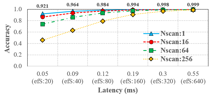
Figure 9: Trade-offs between HNSW routing accuracy and latency on 200K centroids of Deep10M. The y-axis represents the latency in millisecond. $(efS:X)$ in parentheses represents that the latency is obtained with $efSearch$ set to $X$.

7.3.3   Sensitivity of $K$ and $R$

In practice, different applications might require to retrieve different $K$ NNs. Table 4 shows the recall of Zoom at different $K$ and $R$ compared to IVFPQ varying $N_{scan}$ from 1 to 1024 on the Deep10M dataset. We make two observations. First, Zoom offers significant recall improvement for K=1 as well as K > 1. In both cases, the recall of IVFPQ has reached its plateau around 0.60 and 0.70, whereas Zoom consistently brings the recall to $0.98+$. Second, a small $R$ can sharply improve the recall. Although larger $R$ is better for getting higher recall, we observe that further increasing $R$ from 10 to 100 when $K=1$ or from 50 to 100 when $K=10$ does not bring a lot more improvement on recall, indicating that a small $R$ is often sufficient to get high recall.

$N_{scan}$	K=1			K=10
	IVFPQ	Zoom		IVFPQ	Zoom
		R=10	R=100		R=50	R=100
1	0.245	0.291	0.292	0.194	0.200	0.200
4	0.396	0.518	0.521	0.382	0.414	0.414
16	0.519	0.756	0.763	0.559	0.667	0.669
64	0.580	0.906	0.920	0.657	0.864	0.868
256	0.599	0.965	0.983	0.691	0.958	0.966
1024	0.602	0.978	0.998	0.697	0.983	0.994

Table 4: Effect of $K$ and $R$ on recall for IVFPQ and Zoom.

7.3.4   Performance of SSD-assisted reranking

We measure the reranking latency at the full-view step. Without optimizations, it takes 68us to rerank a single candidate vector using synchronous IO without batching. This is slow and it would take a few milliseconds to rerank 100 candidates.

Fig. 10 shows the latency impact of the batched, non-blocking multi-candidate reranking employed by Zoom, varying the size of candidate list $R$ from 10 to 100. For $R$ in this range, we have found that a simple strategy of setting batch size $B$ to $R$ and asynchronous submission count $S$ to 1 already performs much better than synchronous, non-batched reranking. As the candidate list size increases, the reranking time increases almost linearly. With Samsung Pro 960, Zoom can rerank up to 100 candidates of vector length 512-byte in less than 0.6ms. As Zoom requires only a small set of candidates to be reranked, 0.6ms can already cover a good range of $R$.

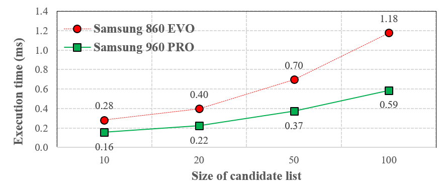
Figure 10: Latency of reranking on two SSDs varying $R$.

We also compare the reranking latency with another SSD Samsung 860 EVO (1TB), to evaluate the sensitivity of the latency on different SSDs. The conclusion still holds for this consumer-grade SSD. The reranking latency roughly get doubled, but it can still rerank 100 candidates in less than 1.2ms. Overall, the results indicate that Zoom can leverage SSDs for the full-view reranking with a small increase on overall latency.

8 Related Work

Tree-based ANN.

One large category of ANN algorithm is tree-based ANN, such as KD-tree [6] and VP-tree [48]. These approaches work well in low dimensions. However, the complexity of these approaches is $O(D\times N^{1-1/D})$, which is not more efficient than a brute-force distance computation at high dimension [29].

Other compact code based approaches.

Another large body of existing ANN work relies on hashing [11, 14], which approximates the similarity between two vectors using hashed codes or Hamming codes. One of the well-known representatives is Locality-Sensitive Hashing (LSH). LSH has the sound probabilistic theoretical guarantees on the query result quality, but product quantization and its extensions combined with inverted file index have been proven to be more effective on large-scale datasets than hashing-based approaches [30, 25].

Hardware accelerators.

Apart from CPU, researchers and practitioners are also looking into using GPU for vector search [23, 42, 47]. However, GPUs also face the same effectiveness and efficiency challenges as their memory is even more limited than CPUs. Although GPUs offer high throughput for offline ANN search, small batch size during online serving can hardly make full usage of massive GPU cores either, rendering low GPU efficiency. Furthermore, people propose to use specialized hardware such as FPGA [49] to serve ANN, but it often requires expert hardware designers and long development cycles to obtain high performance.

9 Conclusion

Vector search becomes instrumental with the major advances in deep learning based feature vector extraction techniques. It is used by many information retrieval services, and it is crucial to conduct search with high accuracy, low latency, and low memory cost. We present Zoom, an ANN solution that employs a multi-view approach and takes the full storage architecture into consideration that greatly enhance the effectiveness and efficiency of ANN search. Zoom uses SSD to maintain full-view vectors and performs reranking on a list of candidates selected by a preview step as an accuracy enhancement procedure. It also improves the overall system efficiency through efficient routing and optimized distance computation. Zoom achieves an order of magnitude improvements on efficiency while attaining equal or higher accuracy, compared with the-state-of-the-art. We conclude that Zoom is a promising approach to ANN. We hope that Zoom will enable future system optimization works on vector search in high dimensional space.

References

- [1] Kernel asynchronous i/o (aio) support for linux, 2018.
- [2] Windows synchronous and asynchronous i/o, 2018.
- [3] Alexandr Andoni, Piotr Indyk, and Ilya Razenshteyn. Approximate Nearest Neighbor Search in High Dimensions. arXiv preprint arXiv:1806.09823, 2018.
- [4] Artem Babenko and Victor S. Lempitsky. Improving Bilayer Product Quantization for Billion-Scale Approximate Nearest Neighbors in High Dimensions. CoRR, abs/1404.1831, 2014.
- [5] Artem Babenko and Victor S. Lempitsky. Efficient Indexing of Billion-Scale Datasets of Deep Descriptors. In 2016 IEEE Conference on Computer Vision and Pattern Recognition, CVPR 2016, Las Vegas, NV, USA, June 27-30, 2016, pages 2055–2063, 2016.
- [6] Jon Louis Bentley. Multidimensional Binary Search Trees Used for Associative Searching. Communications of the ACM, 18(9):509–517, September 1975.
- [7] Google AI Blog. Introducing Semantic Experiences with Talk to Books and Semantris, April 2018.
- [8] Bing blogs. Internet-Scale Deep Learning for Bing Image Search, May 2018.
- [9] Sergey Brin and Lawrence Page. The Anatomy of a Large-scale Hypertextual Web Search Engine. In Proceedings of the Seventh International Conference on World Wide Web 7, WWW7, pages 107–117, Amsterdam, The Netherlands, The Netherlands, 1998. Elsevier Science Publishers B. V.
- [10] B. Barla Cambazoglu and Ricardo Baeza-Yates. Scalability and Efficiency Challenges in Large-scale Web Search Engines. In Proceedings of the 37th International ACM SIGIR Conference on Research & Development in Information Retrieval, SIGIR ’14, pages 1285–1285, New York, NY, USA, 2014. ACM.
- [11] Mayur Datar, Nicole Immorlica, Piotr Indyk, and Vahab S. Mirrokni. Locality-sensitive hashing scheme based on p-stable distributions. In Proceedings of the 20th ACM Symposium on Computational Geometry, Brooklyn, New York, USA, June 8-11, 2004, pages 253–262, 2004.
- [12] Yufei Ding, Yue Zhao, Xipeng Shen, Madanlal Musuvathi, and Todd Mytkowicz. Yinyang k-means: A drop-in replacement of the classic k-means with consistent speedup. In International Conference on Machine Learning, pages 579–587, 2015.
- [13] Wei Dong, Moses Charikar, and Kai Li. Efficient k-nearest neighbor graph construction for generic similarity measures. In Proceedings of the 20th International Conference on World Wide Web, WWW 2011, Hyderabad, India, March 28 - April 1, 2011, pages 577–586, 2011.
- [14] Matthijs Douze, Hervé Jégou, and Florent Perronnin. Polysemous Codes. In Computer Vision - ECCV 2016 - 14th European Conference, Amsterdam, The Netherlands, October 11-14, 2016, Proceedings, Part II, pages 785–801, 2016.
- [15] Tobias Flach, Nandita Dukkipati, Andreas Terzis, Barath Raghavan, Neal Cardwell, Yuchung Cheng, Ankur Jain, Shuai Hao, Ethan Katz-Bassett, and Ramesh Govindan. Reducing Web Latency: The Virtue of Gentle Aggression. In Proceedings of the ACM Conference of the Special Interest Group on Data Communication, SIGCOMM ’13, pages 159–170, 2013.
- [16] Tiezheng Ge, Kaiming He, Qifa Ke, and Jian Sun. Optimized Product Quantization for Approximate Nearest Neighbor Search. In 2013 IEEE Conference on Computer Vision and Pattern Recognition, Portland, OR, USA, June 23-28, 2013, pages 2946–2953, 2013.
- [17] Bob Goodwin, Michael Hopcroft, Dan Luu, Alex Clemmer, Mihaela Curmei, Sameh Elnikety, and Yuxiong He. BitFunnel: Revisiting Signatures for Search. In Proceedings of the 40th International ACM SIGIR Conference on Research and Development in Information Retrieval, SIGIR ’17, pages 605–614, New York, NY, USA, 2017. ACM.
- [18] D. Frank Hsu, Xiaojie Lan, Gabriel Miller, and David Baird. A Comparative Study of Algorithm for Computing Strongly Connected Components. In 15th IEEE Intl Conf on Dependable, Autonomic and Secure Computing, 15th Intl Conf on Pervasive Intelligence and Computing, 3rd Intl Conf on Big Data Intelligence and Computing and Cyber Science and Technology Congress, DASC/PiCom/DataCom/CyberSciTech 2017, Orlando, FL, USA, November 6-10, 2017, pages 431–437, 2017.
- [19] Po-Sen Huang, Xiaodong He, Jianfeng Gao, Li Deng, Alex Acero, and Larry Heck. Learning deep structured semantic models for web search using clickthrough data. In Proceedings of the 22nd ACM international conference on Conference on information & knowledge management, CIKM ’13, pages 2333–2338, New York, NY, USA, 2013. ACM.
- [20] Hamel Husain. How To Create Natural Language Semantic Search For Arbitrary Objects With Deep Learning, May 2018.
- [21] Intel. Storage performance development kit, 2018.
- [22] Herve Jegou, Matthijs Douze, and Cordelia Schmid. Product Quantization for Nearest Neighbor Search. IEEE Transactions on Pattern Analysis and Machine Intelligence, 33(1):117–128, January 2011.
- [23] Jeff Johnson, Matthijs Douze, and Hervé Jégou. Billion-scale similarity search with GPUs. CoRR, abs/1702.08734, 2017.
- [24] Biing-Hwang Juang and Augustine H. Gray Jr. Multiple stage vector quantization for speech coding. In IEEE International Conference on Acoustics, Speech, and Signal Processing, ICASSP ’82, Paris, France, May 3-5, 1982, pages 597–600, 1982.
- [25] Yannis Kalantidis and Yannis S. Avrithis. Locally Optimized Product Quantization for Approximate Nearest Neighbor Search. In 2014 IEEE Conference on Computer Vision and Pattern Recognition, CVPR 2014, Columbus, OH, USA, June 23-28, 2014, pages 2329–2336, 2014.
- [26] Hyeong-Jun Kim, Young-Sik Lee, and Jin-Soo Kim. NVMeDirect: A User-space I/O Framework for Application-specific Optimization on NVMe SSDs. In Proceedings of the 8th USENIX Conference on Hot Topics in Storage and File Systems, HotStorage’16, pages 41–45, Berkeley, CA, USA, 2016. USENIX Association.
- [27] Jon Kleinberg. The Small-world Phenomenon: An Algorithmic Perspective. In Proceedings of the 32 Annual ACM Symposium on Theory of Computing, STOC ’00, pages 163–170, 2000.
- [28] Adaline Lau. Baidu: We Do Semantic Search Better Than Google, May 2018.
- [29] D. T. Lee and C. K. Wong. Worst-case Analysis for Region and Partial Region Searches in Multidimensional Binary Search Trees and Balanced Quad Trees. Acta Informatica, 9(1):23–29, March 1977.
- [30] Wen Li, Ying Zhang, Yifang Sun, Wei Wang, Wenjie Zhang, and Xuemin Lin. Approximate Nearest Neighbor Search on High Dimensional Data - Experiments, Analyses, and Improvement (v1.0). CoRR, abs/1610.02455, 2016.
- [31] Hyeontaek Lim, Bin Fan, David G. Andersen, and Michael Kaminsky. SILT: a memory-efficient, high-performance key-value store. In Proceedings of the 23rd ACM Symposium on Operating Systems Principles 2011, SOSP 2011, Cascais, Portugal, October 23-26, 2011, pages 1–13, 2011.
- [32] Stuart P. Lloyd. Least squares quantization in PCM. IEEE Trans. Information Theory, 28(2):129–136, 1982.
- [33] David G. Lowe. Distinctive Image Features from Scale-Invariant Keypoints. Int. J. Comput. Vision, 60(2):91–110, November 2004.
- [34] Yury Malkov, Alexander Ponomarenko, Andrey Logvinov, and Vladimir Krylov. Approximate nearest neighbor algorithm based on navigable small world graphs. Information Systems, pages 61–68, 2014.
- [35] Yury A. Malkov and D. A. Yashunin. Efficient and robust approximate nearest neighbor search using Hierarchical Navigable Small World graphs. CoRR, arXiv preprint abs/1603.09320, 2016.
- [36] Krishna T. Malladi, Ian Shaeffer, Liji Gopalakrishnan, David Lo, Benjamin C. Lee, and Mark Horowitz. Rethinking DRAM Power Modes for Energy Proportionality. In Proceedings of the 2012 45th Annual IEEE/ACM International Symposium on Microarchitecture, MICRO-45, pages 131–142, Washington, DC, USA, 2012. IEEE Computer Society.
- [37] Miranda Miller. Bing’s New Back-end: Cosmos and Tigers and Scope, Oh My, May 2008.
- [38] Jonas Mueller and Aditya Thyagarajan. Siamese Recurrent Architectures for Learning Sentence Similarity. AAAI’16, pages 2786–2792, 2016.
- [39] Casper Petersen, Jakob Grue Simonsen, and Christina Lioma. Power Law Distributions in Information Retrieval, journal = ACM Trans. Inf. Syst. 34(2):8:1–8:37, February 2016.
- [40] Knut Magne Risvik, Trishul Chilimbi, Henry Tan, Karthik Kalyanaraman, and Chris Anderson. Maguro, a System for Indexing and Searching over Very Large Text Collections. In Proceedings of the Sixth ACM International Conference on Web Search and Data Mining, WSDM ’13, pages 727–736, New York, NY, USA, 2013. ACM.
- [41] Nick Roussopoulos, Stephen Kelley, and Frédéric Vincent. Nearest Neighbor Queries. In Proceedings of the 1995 ACM SIGMOD International Conference on Management of Data, SIGMOD ’95, pages 71–79, 1995.
- [42] Ying Shan, Jian Jiao, Jie Zhu, and J. C. Mao. Recurrent Binary Embedding for GPU-Enabled Exhaustive Retrieval from Billion-Scale Semantic Vectors. CoRR, abs/1802.06466, 2018.
- [43] Junaid Shuja, Kashif Bilal, Sajjad Ahmad Madani, Mazliza Othman, Rajiv Ranjan, Pavan Balaji, and Samee Ullah Khan. Survey of Techniques and Architectures for Designing Energy-Efficient Data Centers. IEEE Systems Journal, 10(2):507–519, 2016.
- [44] Jianguo Wang, Eric Lo, Man Lung Yiu, Jiancong Tong, Gang Wang, and Xiaoguang Liu. The Impact of Solid State Drive on Search Engine Cache Management. In Proceedings of the 36th International ACM SIGIR Conference on Research and Development in Information Retrieval, SIGIR ’13, pages 693–702, New York, NY, USA, 2013. ACM.
- [45] Jianguo Wang, Eric Lo, Man Lung Yiu, Jiancong Tong, Gang Wang, and Xiaoguang Liu. Cache Design of SSD-Based Search Engine Architectures: An Experimental Study. ACM Trans. Inf. Syst., 32(4):21:1–21:26, October 2014.
- [46] Duncan J. Watts. Small Worlds: The Dynamics of Networks Between Order and Randomness. 1999.
- [47] Patrick Wieschollek, Oliver Wang, Alexander Sorkine-Hornung, and Hendrik P. A. Lensch. Efficient Large-scale Approximate Nearest Neighbor Search on the GPU. CoRR, abs/1702.05911, 2017.
- [48] Peter N. Yianilos. Data Structures and Algorithms for Nearest Neighbor Search in General Metric Spaces. In Proceedings of the Fourth Annual ACM-SIAM Symposium on Discrete Algorithms, SODA ’93, pages 311–321, 1993.
- [49] Jialiang Zhang, Soroosh Khoram, and Jing Li. Efficient Large-Scale Approximate Nearest Neighbor Search on OpenCL FPGA. In Proceedings of the IEEE Conference on Computer Vision and Pattern Recognition, pages 4924–4932, 2018.