SNS: a solution-based nonlinear subspace method for time-dependent model order reduction

Abstract

Several reduced order models have been successfully developed for nonlinear dynamical systems. To achieve a considerable speed-up, a hyper-reduction step is needed to reduce the computational complexity due to nonlinear terms. Many hyper-reduction techniques require the construction of nonlinear term basis, which introduces a computationally expensive offline phase. A novel way of constructing nonlinear term basis within the hyper-reduction process is introduced. In contrast to the traditional hyper-reduction techniques where the collection of nonlinear term snapshots is required, the SNS method avoids collecting the nonlinear term snapshots. Instead, it uses the solution snapshots that are used for building a solution basis, which enables avoiding an extra data compression of nonlinear term snapshots. As a result, the SNS method provides a more efficient offline strategy than the traditional model order reduction techniques, such as the DEIM, GNAT, and ST-GNAT methods. The SNS method is theoretically justified by the conforming subspace condition and the subspace inclusion relation. It is useful for model order reduction of large-scale nonlinear dynamical problems to reduce the offline cost. It is especially useful for ST-GNAT that has shown promising results, such as a good accuracy with a considerable online speed-up for hyperbolic problems in a recent paper by Choi and Carlberg in SISC 2019, because ST-GNAT involves an expensive offline cost related to collecting nonlinear term snapshots. Error analysis shows that the oblique projection error bound of the SNS method depends on the condition number of the matrix $\boldsymbol{M}$ (e.g., a volume matrix generated from a discretization of a specific numerical scheme). Numerical results support that the accuracy of the solution from the SNS method is comparable to the traditional methods and a considerable speed-up (i.e., a factor of two to a hundred) is achieved in the offline phase.

1 Introduction

Time-dependent nonlinear problems arise in many important disciplines such as engineering, science, and technologies. They are numerically solved if it is not possible to solve them analytically. Depending on the complexity and size of the governing equations and problem domains, the problems can be computationally expensive to solve. It may take a long time to run one forward simulation even with high performance computing. For example, a simulation of the powder bed fusion additive manufacturing procedure shown in [26] takes a week to finish with $108$ cores. Other computationally expensive simulations include the 3D shocked spherical Helium bubble simulation appeared in [4] and the inertial confinement fusion implosion dynamics simulations appeared in [1]. The computationally expensive simulations are not desirable in the context of parameter study, design optimization, uncertainty quantification, and inverse problems where several forward simulations are needed. A Reduced Order Model (ROM) can be useful in this context to accelerate the computationally expensive forward simulations with good enough approximate solutions.

We consider projection-based ROMs for nonlinear dynamical systems. Such ROMs include the Empirical Interpolation method (EIM) [6, 21], the Discrete Empirical Interpolation Method (DEIM) [12, 15] and the Gauss–Newton with Approximated Tensors [10, 11], the Best Point Interpolation Method (BPIM) [30], the Missing Point Estimation (MPE) [5], and Cubature Methods [3, 19, 20, 23]. There a hyper-reduction (The term first used in the context of ROMs by Ryckelynck in [32]) is necessary to efficiently reduce the complexity of nonlinear terms for a considerable speed-up compared to a corresponding full order model. The DEIM and GNAT approaches take discrete nonlinear term snapshots to build a nonlinear term basis. Then, they select a subset of each nonlinear term basis vector to either interpolate or data-fit in a least-squares sense. In this way, they reduce the computational complexity of updating nonlinear terms in an iterative solver for nonlinear problems. The EIM, BPIM, and MPE approaches take the similar hyper-reduction to the ones in DEIM and GNAT except for the fact that they build nonlinear term basis functions in a continuous space. Whether they work on a discrete or continuous space, they follow the framework of reconstructing “gappy” data, first introduced in the context of reduced order models by [18]. The cubature methods, in contrast, take a different approach. They approximate nonlinear integral as a finite sum of positive scalar weights multiplied by the integrand evaluated at sampled elements. The cubature methods developed in [3, 19, 20] do not require building nonlinear term basis. They solve the Non-Negative Least-Squares (NNLS) problem directly with the nonlinear term snapshots. Recently, Hernandez, et al., in [23] developed the Empirical Cubature Method (ECM) approach that builds nonlinear term basis to solve a smaller NNLS problem. The requirement of building nonlinear term basis in hyper-reduction results in computational cost and storage in addition to solution basis construction. The cost is significant if the corresponding Full Order Models (FOMs) are large-scale. The large-scale problem requires large additional storage for nonlinear term snapshots and large-scale compression techniques to build a basis. In particular, the cost of the hyper-reduction in the recently-developed space–time ROM (i.e., ST-GNAT) [13] is even more significant than aforementioned spatial ROMs (e.g., EIM, DEIM, GNAT, BPIM, MPE, and ECM). The best nonlinear term snapshots of the ST-GNAT method are obtained from the corresponding space–time ROMs without hyper-reduction (i.e., ST-LSPG) [13], which is not practical for a large-scale problem due to the cumbersome size. Therefore, a novel and efficient way of constructing nonlinear term basis needs to be developed.

This paper shows a practical way of avoiding nonlinear term snapshots for the construction of nonlinear term basis. The idea comes from a simple fact that the nonlinear terms are related with solution snapshots through underlying time integrators. In fact, many time integrators approximate time derivative terms as a linear combination of the solution snapshots. It implies that the nonlinear term snapshots belong to the subspace spanned by the solution snapshots. Furthermore, a subspace needed for nonlinear terms in a hyper-reduction is determined by the range space of the solution basis matrix possibly multiplied by a nonsingular matrix (e.g., the volume matrix). Therefore, the solution snapshots can be used to construct nonlinear term basis. This leads to our proposed method, the Solution-based Nonlinear Subspace (SNS) method, that provides two savings for constructing nonlinear term basis because of

1. no additional collection of nonlinear term snapshots (i.e., storage saving).

2. no additional compression of snapshots (e.g., no additional singular value decomposition of nonlinear term snapshots, implying computational cost saving).

The first saving is especially big for GNAT and ST-GNAT becuase they involve expensive collection procedure for their best performace.

1.1 Organization of the paper

We start our discussion by describing the time-continuous representation of the FOM in Section 2. Section 2 also describes the time-discrete representation of the FOM with one-step Euler time integrators. The subspace inclusion relation between the subspaces spanned by the solution and nonlinear term snapshots is described for the Euler time integrators. Several projection-based ROMs (i.e., the DEIM, GNAT, and ST-GNAT models) are considered in Section 3 for the SNS method to be applied. If a reader is familiar with DEIM, GNAT, and ST-GNAT, then the one can skip Section 2 and 3 and start with Section 4. The SNS method is described in Section 4 and applied to those ROMs. Section 4 also introduces the conforming subspace condition to justify the SNS method. Section 5 shows an error analysis for the SNS method regarding the oblique projection error bound. It analyzes the effect of the nonsingular matrix that is used to form a nonlinear term basis. Section 6 reports numerical results that support benefits of the SNS method and Section 7 concludes the paper with summary and future work. Although the SNS method is mainly illustrated with the Euler time integrators throughout the paper, it is applicable to other time integrators. Appendix A considers several other time integrators and the subspace inclusion relation for each time integrator. The following time integrators are included: the Adams–Bashforth, Adams–Moulton, BDF, and midpoint Runge–Kutta methods.

2 Full order model

A parameterized nonlinear dynamical system is considered, characterized by a system of nonlinear ordinary differential equations (ODEs), which can be considered as a resultant system from semi-discretization of Partial Differential Equations (PDEs) in space domains

(2.1) $$\boldsymbol{M}\frac{d\boldsymbol{x}}{dt}=\boldsymbol{f}(\boldsymbol{x},t;\boldsymbol{\mu}),\quad\quad\boldsymbol{x}(0;\boldsymbol{\mu})=\boldsymbol{x}^{0}(\boldsymbol{\mu}),$$

where $\boldsymbol{M}\in\mathbb{R}^{N_{s}\times N_{s}}$ denotes a nonsingular matrix, $t\in[0,T]$ denotes time with the final time $T\in\mathbb{R}_{+}$, and $\boldsymbol{x}(t;\boldsymbol{\mu})$ denotes the time-dependent, parameterized state implicitly defined as the solution to problem (2.1) with $\boldsymbol{x}:[0,T]\times\mathcal{D}\rightarrow\mathbb{R}^{N_{s}}$. Further, $\boldsymbol{f}:\mathbb{R}^{N_{s}}\times[0,T]\times\mathcal{D}\rightarrow\mathbb{R}^{N_{s}}$ with $(\boldsymbol{w},\tau;\boldsymbol{\nu})\mapsto\boldsymbol{f}(\boldsymbol{w},\tau;\boldsymbol{\nu})$ denotes the scaled velocity of $\boldsymbol{M}\boldsymbol{x}$, which we assume to be nonlinear in at least its first argument. The initial state is denoted by $\boldsymbol{x}^{0}:\mathcal{D}\rightarrow\mathbb{R}^{N_{s}}$, and $\boldsymbol{\mu}\in\mathcal{D}$ denotes the parameters with parameter domain $\mathcal{D}\subseteq\mathbb{R}^{n_{\mu}}$.

A uniform time discretization is assumed throughout the paper, characterized by time step $\Delta t\in\mathbb{R}_{+}$ and time instances $t^{n}=t^{n-1}+\Delta t$ for $n\in{\rm Nature}{{N_{t}}}$ with $t^{0}=0$, ${N_{t}}\in\mathbb{N}$, and ${\rm Nature}{N}:=\{1,\ldots,N\}$. To avoid notational clutter, we introduce the following time discretization-related notations: $\boldsymbol{x}_{n}:=\boldsymbol{x}(t^{n};\boldsymbol{\mu})$, $\tilde{\boldsymbol{x}}_{n}:=\tilde{\boldsymbol{x}}(t^{n};\boldsymbol{\mu})$, $\hat{\boldsymbol{x}}_{n}:=\hat{\boldsymbol{x}}(t^{n};\boldsymbol{\mu})$, and $\boldsymbol{f}_{n}:=\boldsymbol{f}(\boldsymbol{x}(t^{n};\boldsymbol{\mu}),t^{n};\boldsymbol{\mu})$.

Two different types of time discretization methods are considered: explicit and implicit time integrators. As an illustration purpose, we mainly consider the forward Euler time integrator for an explicit scheme and the backward Euler time integrator for an implicit scheme. Several other time integrators are shown in Appendix A.

The explicit Forward Euler (FE) method numerically solves Eq. (2.1), by time-marching with the following update:

(2.2) $$\boldsymbol{M}\boldsymbol{x}_{n}-\boldsymbol{M}\boldsymbol{x}_{n-1}=\Delta t\boldsymbol{f}_{n-1}.$$

Eq. (2.2) implies the following subspace inclusion:

(2.3) $$\mathrm{span}\{\boldsymbol{f}_{n-1}\}\subseteq\mathrm{span}\{\boldsymbol{M}\boldsymbol{x}_{n-1},\boldsymbol{M}\boldsymbol{x}_{n}\}.$$

By induction, we conclude the following subspace inclusion relation:

(2.4) $$\mathrm{span}\{\boldsymbol{f}_{0},\dots,\boldsymbol{f}_{{N_{t}}-1}\}\subseteq\mathrm{span}\{\boldsymbol{M}\boldsymbol{x}_{0},\ldots,\boldsymbol{M}\boldsymbol{x}_{{N_{t}}}\},$$

which shows that the span of nonlinear term snapshots is included in the span of $\boldsymbol{M}$-scaled solution snapshots. The residual function with the forward Euler time integrator is defined as

(2.5) $$\begin{split}\boldsymbol{r}^{n}_{\mathrm{FE}}(\boldsymbol{x}_{n};\boldsymbol{x}_{n-1},\boldsymbol{\mu})&:=\boldsymbol{M}(\boldsymbol{x}_{n}-\boldsymbol{x}_{n-1})-\Delta t\boldsymbol{f}_{n-1}\end{split}$$

The implicit Backward Euler (BE) method numerically solves Eq. (2.1), by solving the following nonlinear system of equations for $\boldsymbol{x}_{n}$ at $n$-th time step:

(2.6) $$\boldsymbol{M}\boldsymbol{x}_{n}-\boldsymbol{M}\boldsymbol{x}_{n-1}=\Delta t\boldsymbol{f}_{n}.$$

Eq. (2.6) implies the following subspace inclusion:

(2.7) $$\mathrm{span}\{\boldsymbol{f}_{n}\}\subseteq\mathrm{span}\{\boldsymbol{M}\boldsymbol{x}_{n-1},\boldsymbol{M}\boldsymbol{x}_{n}\}.$$

By induction, we conclude the following subspace inclusion relation:

(2.8) $$\mathrm{span}\{\boldsymbol{f}_{1},\dots,\boldsymbol{f}_{{N_{t}}}\}\subseteq\mathrm{span}\{\boldsymbol{M}\boldsymbol{x}_{0},\ldots,\boldsymbol{M}\boldsymbol{x}_{{N_{t}}}\},$$

which shows that the span of nonlinear term snapshots is included in the span of $\boldsymbol{M}$-scaled solution snapshots. The residual function with the backward Euler time integrator is defined as

(2.9) $$\begin{split}\boldsymbol{r}^{n}_{\mathrm{BE}}(\boldsymbol{x}_{n};\boldsymbol{x}_{n-1},\boldsymbol{\mu})&:=\boldsymbol{M}(\boldsymbol{x}_{n}-\boldsymbol{x}_{n-1})-\Delta t\boldsymbol{f}_{n}.\end{split}$$

3 Projection-based reduced order models

Projection-based reduced order models are considered for nonlinear dynamical systems. Especially, the ones that require building a nonlinear term basis are of our interest: the DEIM, GNAT, and ST-GNAT approaches.

3.1 DEIM

The DEIM approach applies spatial projection using a subspace $\mathcal{S}:=\mathrm{span}\{\boldsymbol{\phi}_{i}\}_{i=1}^{n_{s}}\subseteq\mathbb{R}^{N_{s}}$ with $\dim(\mathcal{S})={n_{s}}\ll N_{s}$. Using this subspace, it approximates the solution as $\boldsymbol{x}\approx\tilde{\boldsymbol{x}}\in\boldsymbol{x}_{0}+\mathcal{S}$ (i.e., in a trial subspace) or equivalently

(3.1) $$\tilde{\boldsymbol{x}}=\boldsymbol{x}_{0}+\boldsymbol{\Phi}\hat{\boldsymbol{x}}$$

where $\boldsymbol{\Phi}:=[\boldsymbol{\phi}_{1}\cdots\boldsymbol{\phi}_{{n_{s}}}]\in\mathbb{R}^{N_{s}\times{n_{s}}}$ denotes a basis matrix and $\hat{\boldsymbol{x}}\in\mathbb{R}^{{n_{s}}}$ with $\hat{\boldsymbol{x}}_{0}={\boldsymbol{0}}$ denotes the generalized coordinates. Replacing $\boldsymbol{x}$ with $\tilde{\boldsymbol{x}}$ in Eq. (2.1) leads to the following system of equations with reduced number of unknowns:

(3.2) $$\boldsymbol{M}\boldsymbol{\Phi}\frac{d\hat{\boldsymbol{x}}}{dt}=\boldsymbol{f}(\boldsymbol{x}_{0}+\boldsymbol{\Phi}\hat{\boldsymbol{x}},t;\boldsymbol{\mu}).$$

For constructing $\boldsymbol{\Phi}$, Proper Orthogonal Decomposition (POD) is commonly used. POD [7] obtains $\boldsymbol{\Phi}$ from a truncated Singular Value Decomposition (SVD) approximation to a FOM solution snapshot matrix. It is related to principal component analysis in statistical analysis [25] and Karhunen–Loève expansion [28] in stochastic analysis. POD forms a solution snapshot matrix, $\boldsymbol{X}:=\begin{bmatrix}\boldsymbol{x}_{0}^{\boldsymbol{\mu}_{1}}&\cdots&\boldsymbol{x}_{{N_{t}}}^{\boldsymbol{\mu}_{n_{\mu}}}\end{bmatrix}\in\mathbb{R}^{N_{s}\times n_{\mu}({N_{t}}+1)}$, where $\boldsymbol{x}_{n}^{\boldsymbol{\mu}_{k}}$ is a solution state at $n$th time step with parameter $\boldsymbol{\mu}_{k}$ for $n\in{\rm Nature}{{N_{t}}}$ and $k\in{\rm Nature}{n_{\mu}}$. Then, POD computes its thin SVD:

(3.3) $$\boldsymbol{X}=\boldsymbol{U}\boldsymbol{\Sigma}\boldsymbol{V}^{T},$$

where $\boldsymbol{U}\in\mathbb{R}^{N_{s}\times{N_{t}}}$ and $\boldsymbol{V}\in\mathbb{R}^{{N_{t}}\times{N_{t}}}$ are orthogonal matrices and $\boldsymbol{\Sigma}\in\mathbb{R}^{{N_{t}}\times{N_{t}}}$ is a diagonal matrix with singular values on its diagonals. Then POD chooses the leading ${n_{s}}$ columns of $\boldsymbol{U}$ to set $\boldsymbol{\Phi}$ (i.e., $\boldsymbol{\Phi}=\boldsymbol{U}(:,1:{n_{s}})$ in MATLAB notation). The POD basis minimizes $\|\boldsymbol{X}-\boldsymbol{\Phi}\boldsymbol{\Phi}^{T}\boldsymbol{X}\|_{F}^{2}$ over all $\boldsymbol{\Phi}\in\mathbb{R}^{N_{s}\times{n_{s}}}$ with orthonormal columns, where $\|\boldsymbol{A}\|_{F}$ denotes the Frobenius norm of a matrix $\boldsymbol{A}\in\mathbb{R}^{I\times J}$, defined as $\|\boldsymbol{A}\|_{F}=\sqrt{\sum_{i=1}^{I}\sum_{j=1}^{J}a_{ij}}$ with $a_{ij}$ being an $(i,j)$-th element of $\boldsymbol{A}$. Since the objective function does not change if $\boldsymbol{\Phi}$ is post-multiplied by an arbitrary ${n_{s}}\times{n_{s}}$ orthogonal matrix, the POD procedure seeks the optimal ${n_{s}}$–-dimensional subspace that captures the snapshots in the least-squares sense. For more details on POD, we refer to [24, 27].

Note that Eq. (3.2) has more equations than unknowns (i.e., an overdetermined system). It is likely that there is no solution satisfying Eq. (3.2). In order to close the system, the Galerkin projection solves the following reduced system with $\hat{\boldsymbol{x}}_{0}={\boldsymbol{0}}$:

(3.4) $$\boldsymbol{\Phi}^{T}\boldsymbol{M}\boldsymbol{\Phi}\frac{d\hat{\boldsymbol{x}}}{dt}=\boldsymbol{\Phi}^{T}\boldsymbol{f}(\boldsymbol{x}_{0}+\boldsymbol{\Phi}\hat{\boldsymbol{x}},t;\boldsymbol{\mu}).$$

Applying a time integrator to Eq. (3.4) leads to a fully discretized reduced system, denoted as the reduced O$\Delta$E. Note that the reduced O$\Delta$E has ${n_{s}}$ unknowns and ${n_{s}}$ equations. If an implicit time integrator is applied, a Newton–type method can be applied to solve for unknown generalized coordinates each time step. If an explicit time integrator is applied, time marching updates will solve the system. However, we cannot expect any speed-up because the size of the nonlinear term $\boldsymbol{f}$ and its Jacobian, which need to be updated for every Newton step, scales with the FOM size. Thus, to overcome this issue, the DEIM approach applies a hyper-reduction technique. That is, it projects $\boldsymbol{f}$ onto a subspace $\mathcal{F}:=\mathrm{span}\{\boldsymbol{\phi}_{f,{i}}\}_{i=1}^{n_{f}}$ and approximates $\boldsymbol{f}$ as

(3.5) $$\boldsymbol{f}\approx\boldsymbol{\Phi}_{f}\hat{\boldsymbol{f}},$$

where $\boldsymbol{\Phi}_{f}:=[\boldsymbol{\phi}_{f,{1}},\ldots,\boldsymbol{\phi}_{f,{n_{f}}}]\in\mathbb{R}^{N_{s}\times n_{f}}$, $n_{f}\ll N_{s}$, denotes the nonlinear term basis matrix and $\hat{\boldsymbol{f}}\in\mathbb{R}^{n_{f}}$ denotes the generalized coordinates of the nonlinear term. The generalized coordinates, $\hat{\boldsymbol{f}}$, can be determined by the following interpolation:

(3.6) $$\boldsymbol{Z}^{T}\boldsymbol{f}=\boldsymbol{Z}^{T}\boldsymbol{\Phi}_{f}\hat{\boldsymbol{f}},$$

where $\boldsymbol{Z}^{T}:=[{\boldsymbol{e}}_{p_{1}},\ldots,{\boldsymbol{e}}_{p_{n_{f}}}]^{T}\in\mathbb{R}^{n_{f}\times N_{s}}$ is the sampling matrix and ${\boldsymbol{e}}_{p_{i}}$ is the $p_{i}$th column of the identity matrix $\boldsymbol{I}_{N_{s}}\in\mathbb{R}^{N_{s}\times N_{s}}$. Therefore, Eq. (3.5) becomes

(3.7) $$\boldsymbol{f}\approx\mathcal{P}_{\text{DEIM}}\boldsymbol{f},$$

where $\mathcal{P}_{\text{DEIM}}:=\boldsymbol{\Phi}_{f}(\boldsymbol{Z}^{T}\boldsymbol{\Phi}_{f})^{-1}\boldsymbol{Z}^{T}\in\mathbb{R}^{n_{f}\times n_{f}}$ is the DEIM oblique projection matrix. The DEIM approach does not construct the sampling matrix $\boldsymbol{Z}$. Instead, it maintains the sampling indices $\{p_{1},\ldots,p_{n_{f}}\}$ and corresponding rows of $\boldsymbol{\Phi}_{f}$ and $\boldsymbol{f}$. This enables DEIM to achieve a speed-up when it is applied to nonlinear problems.

The original DEIM paper [12] constructs the nonlinear term basis $\{\boldsymbol{\phi}_{f,{1}},\ldots,\boldsymbol{\phi}_{f,{n_{f}}}\}$ by applying another POD on the nonlinear term snapshots obtained from the FOM simulation at every time step. This implies that DEIM requires two separate SVDs and storage for two different snapshots (i.e., solution state and nonlinear term snapshots). Section 4 discusses how to avoid the collection of nonlinear term snapshots and an extra SVD without losing the quality of the hyper-reduction.

The sampling indices (i.e., $\boldsymbol{Z}$) can be found either by a row pivoted LU decomposition [12] or the strong column pivoted rank-revealing QR (sRRQR) decomposition [15, 16]. Depending on the algorithm of selecting the sampling indices, the DEIM projection error bound is determined. For example, the row pivoted LU decomposition in [12] results in the following error bound:

(3.8) $$\|\boldsymbol{f}-\mathcal{P}\boldsymbol{f}\|_{2}\leq\kappa\|(\boldsymbol{I}_{N_{s}}-\boldsymbol{\Phi}_{f}\boldsymbol{\Phi}_{f}^{T})\boldsymbol{f}\|_{2},$$

where $\|\cdot\|_{2}$ denotes $\ell_{2}$ norm of a vector and $\kappa$ is the condition number of $(\boldsymbol{Z}^{T}\boldsymbol{\Phi}_{f})^{-1}$ and it is bounded by

(3.9) $$\kappa\leq(1+\sqrt{2N_{s}})^{n_{f}-1}\|\boldsymbol{\phi}_{f,{1}}\|_{\infty}^{-1}.$$

On the other hand, the sRRQR factorization in [16] reveals tighter bound than (3.9):

(3.10) $$\kappa\leq\sqrt{1+\eta^{2}n_{f}(N_{s}-n_{f})}$$

where $\eta$ is a tuning parameter in the sRRQR factorization (i.e., $f$ in Algorithm 4 of [22]).

3.2 GNAT

In contrast to DEIM, the GNAT method takes the Least-Squares Petrov–Galerkin (LSPG) approach. The LSPG method projects a fully discretized solution space onto a trial subspace. That is, it discretizes Eq. (2.1) in time domain and replaces $\boldsymbol{x}_{n}$ with $\tilde{\boldsymbol{x}}_{n}:=\boldsymbol{x}_{0}+\boldsymbol{\Phi}\hat{\boldsymbol{x}}_{n}$ for $n\in{\rm Nature}{{N_{t}}}$ in residual functions defined in Section 2 and Appendix A. Here, we consider only implicit time integrators because the LSPG projection is equivalent to the Galerkin projection when an explicit time integrator is used as shown in Section 5.1 in [9]. The residual functions for implicit time integrators are defined in (2.9), (A.8), and (A.12) for various time integrators. For example, the residual function with the backward Euler time integrator after the trial subspace projection becomes

(3.11) $$\begin{split}\tilde{\boldsymbol{{\mathsf{r}}}}^{n}_{\mathrm{BE}}(\hat{\boldsymbol{x}}_{n};\hat{\boldsymbol{x}}_{n-1},\boldsymbol{\mu})&:=\boldsymbol{r}^{n}_{\mathrm{BE}}(\boldsymbol{x}_{0}+\boldsymbol{\Phi}\hat{\boldsymbol{x}}_{n};\boldsymbol{x}_{0}+\boldsymbol{\Phi}\hat{\boldsymbol{x}}_{n-1},\boldsymbol{\mu})\\ &=\boldsymbol{M}\boldsymbol{\Phi}(\hat{\boldsymbol{x}}_{n}-\hat{\boldsymbol{x}}_{n-1})-\Delta t\boldsymbol{f}(\boldsymbol{x}_{0}+\boldsymbol{\Phi}\hat{\boldsymbol{x}}_{n},t;\boldsymbol{\mu}).\end{split}$$

The basis matrix $\boldsymbol{\Phi}$ can be found by the POD as in the DEIM approach. Note that Eq. (3.11) is an over-determined system. To close the system and solve for the unknown generalized coordinates, $\hat{\boldsymbol{x}}_{n}$, the LSPG ROM takes the squared norm of the residual vector function and minimize it at every time step:

(3.12) $$\begin{split}\hat{\boldsymbol{x}}_{n}=\underset{\hat{\boldsymbol{v}}\in\mathbb{R}^{{n_{s}}}}{\text{argmin}}\quad&\frac{1}{2}\left\|\boldsymbol{r}^{n}_{\mathrm{BE}}(\hat{\boldsymbol{v}};\hat{\boldsymbol{x}}_{n-1},\boldsymbol{\mu})\right\|_{2}^{2}.\end{split}$$

The Gauss–Newton method with the starting point $\hat{\boldsymbol{x}}_{n-1}$ is applied to solve the minimization problem (3.12) in GNAT. However, as in the DEIM approach, a hyper-reduction is required for a speed-up due to the presence of the nonlinear residual vector function. The GNAT method approximates the nonlinear residual term with gappy POD [18], whose procedure is similar to DEIM, as

(3.13) $$\boldsymbol{r}\approx\boldsymbol{\Phi}_{r}\hat{\boldsymbol{r}},$$

where $\boldsymbol{\Phi}_{r}:=[\boldsymbol{\phi}_{r,1},\ldots,\boldsymbol{\phi}_{r,n_{r}}]\in\mathbb{R}^{N_{s}\times n_{r}}$, ${n_{s}}\leq n_{r}\ll N_{s}$, denotes the residual basis matrix and $\hat{\boldsymbol{r}}\in\mathbb{R}^{n_{r}}$ denotes the generalized coordinates of the nonlinear residual term. In contrast to DEIM, the GNAT method solves the following least-squares problem to obtain the generalized coordinates $\hat{\boldsymbol{r}}_{n}$ at $n$-th time step:

(3.14) $$\begin{split}\hat{\boldsymbol{r}}_{n}=\underset{\hat{\boldsymbol{v}}\in\mathbb{R}^{n_{r}}}{\text{argmin}}\quad&\frac{1}{2}\left\|\boldsymbol{Z}^{T}(\boldsymbol{r}-\boldsymbol{\Phi}_{r}\hat{\boldsymbol{v}})\right\|_{2}^{2}.\end{split}$$

where $\boldsymbol{Z}^{T}:=[{\boldsymbol{e}}_{p_{1}},\ldots,{\boldsymbol{e}}_{p_{n_{z}}}]^{T}\in\mathbb{R}^{n_{z}\times N_{s}}$, ${n_{s}}\leq n_{r}\leq n_{z}\ll N_{s}$, is the sampling matrix and ${\boldsymbol{e}}_{p_{i}}$ is the $p_{i}$th column of the identity matrix $\boldsymbol{I}_{N_{s}}\in\mathbb{R}^{N_{s}\times N_{s}}$. The solution to Eq. (3.14) is given as

(3.15) $$\hat{\boldsymbol{r}}_{n}=(\boldsymbol{Z}^{T}\boldsymbol{\Phi}_{r})^{\dagger}\boldsymbol{Z}^{T}\boldsymbol{r},$$

where the Moore–Penrose inverse of a matrix $\boldsymbol{A}\in\mathbb{R}^{n_{z}\times n_{r}}$ with full column rank is defined as $\boldsymbol{A}^{\dagger}:=(\boldsymbol{A}^{T}\boldsymbol{A})^{-1}\boldsymbol{A}^{T}$. Therefore, Eq. (3.13) becomes

(3.16) $$\boldsymbol{r}\approx\mathcal{P}_{\text{GNAT}}\boldsymbol{r},$$

where $\mathcal{P}_{\text{GNAT}}:=\boldsymbol{\Phi}_{r}(\boldsymbol{Z}^{T}\boldsymbol{\Phi}_{r})^{\dagger}\boldsymbol{Z}^{T}$ is the GNAT oblique projection matrix. Note that it has a similar structure to $\mathcal{P}_{\text{DEIM}}$. The GNAT projection matrix has a pseudo-inverse instead of the inverse becuase it allows $n_{r}<n_{z}$. The GNAT method does not construct the sampling matrix $\boldsymbol{Z}$. Instead, it maintains the sampling indices $\{p_{1},\ldots,p_{n_{f}}\}$ and corresponding rows of $\boldsymbol{\Phi}_{r}$ and $\boldsymbol{r}$. This enables GNAT to achieve a speed-up when it is applied to nonlinear problems.

The sampling indices (i.e., $\boldsymbol{Z}$) can be determined by Algorithm 3 of [11] for computational fluid dynamics problems and Algorithm 5 of [10] for other problems. These two algorithms take greedy procedure to minimize the error in the gappy reconstruction of the POD basis vectors $\boldsymbol{\Phi}_{r}$. The major difference between these sampling algorithms and the ones for the DEIM method is that these algorithms for the GNAT method allows oversampling (i.e., $n_{z}>n_{r}$), resulting in solving least-squares problems in the greedy procedure. These selection algorithms can be viewed as the extension of Algorithm 1 in [12] (i.e., a row pivoted LU decomposition) to the oversampling case. The nonlinaer residual term projection error associated with these sampling algorithms is presented in Appendix D of [11]. That is,

(3.17) $$\|\boldsymbol{r}-\mathcal{P}_{\text{GNAT}}\boldsymbol{r}\|_{2}\leq\|\boldsymbol{R}^{-1}\|_{2}\|\boldsymbol{r}-\boldsymbol{\Phi}_{r}\boldsymbol{\Phi}_{r}^{T}\boldsymbol{r}\|_{2}$$

where $\boldsymbol{R}$ is the triangular factor from the QR factorization of $\boldsymbol{Z}^{T}\boldsymbol{\Phi}_{r}$ (i.e., $\boldsymbol{Z}^{T}\boldsymbol{\Phi}_{r}=\boldsymbol{Q}\boldsymbol{R}$).

We present another sampling selection algorithm that was not considered in any GNAT papers (e.g., [10, 11]). It is to use the sRRQR factorization developed originally in [22] and further utilized in the W-DEIM method of [16] for the case of $n_{z}\geq n_{r}$. That is, applying Algorithm 4 of [22] to $\boldsymbol{\Phi}_{r}^{T}$ produces an index selection operator $\boldsymbol{Z}$ whose projection error satisfies

(3.18) $$\|\boldsymbol{r}-\mathcal{P}_{\text{GNAT}}\boldsymbol{r}\|_{2}\leq\sqrt{1+\eta^{2}n_{r}(N_{s}-n_{r})}\|\boldsymbol{r}-\boldsymbol{\Phi}_{r}\boldsymbol{\Phi}_{r}^{T}\boldsymbol{r}\|_{2}.$$

This error bound can be obtained by setting the identity matrix as a weight matrix in Theorem 4.8 of [16].

Finally, the GNAT method minimizes the following least-squares problem at every time step, for example, with the backward Euler time integrator:

(3.19) $$\begin{split}\hat{\boldsymbol{x}}_{n}=\underset{\hat{\boldsymbol{v}}\in\mathbb{R}^{{n_{s}}}}{\text{argmin}}\quad&\frac{1}{2}\left\|\ (\boldsymbol{Z}^{T}\boldsymbol{\Phi}_{r})^{\dagger}\boldsymbol{Z}^{T}\boldsymbol{r}^{n}_{\mathrm{BE}}(\hat{\boldsymbol{v}};\hat{\boldsymbol{x}}_{n-1},\boldsymbol{\mu})\right\|_{2}^{2}.\end{split}$$

The GNAT method applies another POD to a nonlinear residual term snapshots to construct $\boldsymbol{\Phi}_{r}$. The original GNAT paper [11] collects residual snapshots at every Newton iteration from the LSPG simulations for several reasons:

1. The GNAT method takes LSPG as a reference model (i.e., denoted as Model II in [11]). Its ultimate goal is to achieve the accuracy of Model II.

2. The residual snapshots taken every time step (i.e., at the end of Newton iterations at every time step) of the FOM are small in magnitude.

3. The residual snapshots taken from every Newton step gives information about the path that the Newton iterations in Model II take. GNAT tries to mimic the Newton path that LSPG takes.

Some disadvantages of the original GNAT approach include:

1. The GNAT method requires more storage than DEIM to store residual snapshots from every Newton iteration (cf., The DEIM approach stores only one nonlinear term snapshot per each time step).

2. The GNAT method requires more expensive SVD for nonlinear residual basis construction than the DEIM approach because the number of nonlinear residual snapshots in the GNAT method is larger than the number of nonlinear term snapshots in DEIM.

3. The GNAT method requires the simulations of Model II which are computationally expensive. For a parametric global ROM, it is computationally expensive because it requires as many Model II simulations as there are training points in a given parameter domain.

Section 4 discusses how to avoid the collection of nonlinear term snapshots and the extra SVD without losing the quality of the hyper-reduction.

3.3 Space–time GNAT

The ST-GNAT method takes the space–time LSPG (ST-LSPG) approach. Given a time integrator, one can rewrite a fully discretized system of equations to Eq. (2.1) in a space–time form. For example, if the backward Euler time integrator is used for time domain discretization, then the corresponding space–time formulation to Eq. (2.6) becomes

(3.20) $$\boldsymbol{A}_{\text{BE}}\bar{\boldsymbol{x}}=\Delta t\bar{\boldsymbol{f}}+\bar{\boldsymbol{q}}^{0},$$

where

(3.21) $$\boldsymbol{A}_{\text{BE}}=\begin{bmatrix}\boldsymbol{M}&&&\\ -\boldsymbol{M}&\boldsymbol{M}&&\\ &\ddots&\ddots&\\ &&-\boldsymbol{M}&\boldsymbol{M}\end{bmatrix},\quad\bar{\boldsymbol{x}}=\begin{pmatrix}\boldsymbol{x}_{1}\\ \boldsymbol{x}_{2}\\ \vdots\\ \boldsymbol{x}_{{N_{t}}}\end{pmatrix},\quad\bar{\boldsymbol{f}}=\begin{pmatrix}\boldsymbol{f}_{1}\\ \boldsymbol{f}_{2}\\ \vdots\\ \boldsymbol{f}_{{N_{t}}}\end{pmatrix},\quad\bar{\boldsymbol{q}}^{0}=\begin{pmatrix}\boldsymbol{M}\boldsymbol{x}^{0}\\ {\bf 0}\\ \vdots\\ {\bf 0}\end{pmatrix}.$$

Note that $\bar{\boldsymbol{x}}(\boldsymbol{\mu})$ denotes the parameterized space–time state implicitly defined as the solution to the problem (3.20) with $\bar{\boldsymbol{x}}:\mathcal{D}\rightarrow\mathbb{R}^{N_{s}{N_{t}}}$ and $\bar{\boldsymbol{x}}(\boldsymbol{\mu})\in\mathbb{R}^{N_{s}{N_{t}}}$. Further, $\bar{\boldsymbol{f}}(\bar{\boldsymbol{x}};\boldsymbol{\mu})\in\mathbb{R}^{N_{s}{N_{t}}}$ denotes the space–time nonlinear term that is nonlinear in at least its first argument with $\bar{\boldsymbol{f}}:\mathbb{R}^{N_{s}{N_{t}}}\times\mathcal{D}\rightarrow\mathbb{R}^{N_{s}{N_{t}}}$. The space–time residual function $\boldsymbol{\bar{r}}\in\mathbb{R}^{N_{s}{N_{t}}}$ corresponding to Eq. (3.20) is defined as

(3.22) $$\begin{split}\boldsymbol{\bar{r}}_{\text{BE}}(\bar{\boldsymbol{x}};\boldsymbol{\mu})&:=\boldsymbol{A}_{\text{BE}}\bar{\boldsymbol{x}}(\boldsymbol{\mu})-\Delta t\bar{\boldsymbol{f}}(\bar{\boldsymbol{x}};\boldsymbol{\mu})-\bar{\boldsymbol{q}}^{0}(\boldsymbol{\mu}).\\ &={\bf 0}\end{split}$$

To reduce both the spatial and temporal dimensions of the full-order model, the ST-LSPG method enforces the approximated numerical solution $\tilde{\boldsymbol{y}}\in\mathbb{R}^{N_{s}{N_{t}}}$ to reside in an affine ‘space–time trial subspace’

(3.23) $$\tilde{\boldsymbol{y}}\in\mathcal{ST}\subseteq\mathbb{R}^{N_{s}{N_{t}}},$$

where $\mathcal{ST}:=\boldsymbol{1}_{{N_{t}}}\otimes\boldsymbol{x}^{0}(\boldsymbol{\mu})+\mathrm{span}\{\bar{\boldsymbol{\phi}}_{i}\}_{i=1}^{n_{st}}\subseteq\mathbb{R}^{N_{s}{N_{t}}}$ with $\dim(\mathcal{ST})={n_{st}}\ll N_{s}{N_{t}}$ and $\boldsymbol{1}_{{N_{t}}}\in\mathbb{R}^{{N_{t}}}$ whose elements are all one. Here, $\otimes$ denotes the Kronecker product of two matrices and the product of two matrices $\boldsymbol{A}\in\mathbb{R}^{I\times J}$ and $\boldsymbol{B}\in\mathbb{R}^{K\times L}$ is defined as

(3.24) $$\boldsymbol{A}\otimes\boldsymbol{B}=\begin{bmatrix}a_{11}\boldsymbol{B}&\cdots&a_{1J}\boldsymbol{B}\\ \vdots&\ddots&\vdots\\ a_{I1}\boldsymbol{B}&\cdots&a_{IJ}\boldsymbol{B}\end{bmatrix}.$$

Further, $\bar{\boldsymbol{\phi}}_{i}\in\mathbb{R}^{N_{s}{N_{t}}}$ denotes a space–time basis vector. Thus, the ST-LSPG method approximates the numerical solution as

(3.25) $$\begin{split}\bar{\boldsymbol{x}}(\boldsymbol{\mu})\approx\tilde{\boldsymbol{y}}(\boldsymbol{\mu})&=\boldsymbol{1}_{{N_{t}}}\otimes\boldsymbol{x}^{0}(\boldsymbol{\mu})+\sum_{i=1}^{{n_{st}}}\bar{\boldsymbol{\phi}}_{i}\hat{y}_{i}(\boldsymbol{\mu})\end{split}$$

where $\hat{y}_{i}(\boldsymbol{\mu})\in\mathbb{R}$, $i\in{\rm Nature}{{n_{st}}}$ denotes the generalized coordinate of the ST-LSPG solution.

A space–time residual vector function can now be defined with the generalized coordinates as an argument. Replacing $\bar{\boldsymbol{x}}$ in Eq. (3.22) with $\tilde{\boldsymbol{y}}$ gives the residual vector function

(3.26) $$\boldsymbol{\bar{{\mathsf{r}}}}_{\text{BE}}(\hat{\boldsymbol{y}};\boldsymbol{\mu}):=\boldsymbol{A}_{\text{BE}}\bar{\boldsymbol{\Phi}}\hat{\boldsymbol{y}}-\Delta t\bar{\boldsymbol{f}}(\bar{\boldsymbol{x}}^{0}+\bar{\boldsymbol{\Phi}}\hat{\boldsymbol{y}};\boldsymbol{\mu})-\bar{\boldsymbol{q}}^{0}(\boldsymbol{\mu})+\boldsymbol{A}_{\text{BE}}\bar{\boldsymbol{x}}^{0}(\boldsymbol{\mu}),$$

where $\bar{\boldsymbol{x}}^{0}:=\boldsymbol{1}_{{N_{t}}}\otimes\boldsymbol{x}^{0}$ and $\bar{\boldsymbol{\Phi}}\in\mathbb{R}^{N_{s}{N_{t}}\times{n_{st}}}$ denotes a space–time basis matrix that is defined as $\bar{\boldsymbol{\Phi}}:=\begin{bmatrix}\bar{\boldsymbol{\phi}}_{1}&\cdots&\bar{\boldsymbol{\phi}}_{{n_{st}}}\end{bmatrix}$ and $\hat{\boldsymbol{y}}\in\mathbb{R}^{{n_{st}}}$ denotes the generalized coordinate vector that is defined as

(3.27) $$\hat{\boldsymbol{y}}:=\begin{bmatrix}\hat{y}_{1}(\boldsymbol{\mu})&\cdots&\hat{y}_{{n_{st}}}(\boldsymbol{\mu})\end{bmatrix}^{T}.$$

Note that $\bar{\boldsymbol{q}}^{0}(\boldsymbol{\mu})+\boldsymbol{A}_{\text{BE}}\bar{\boldsymbol{x}}^{0}(\boldsymbol{\mu})$ vanishes. Eq. (3.26) becomes

(3.28) $$\boldsymbol{\bar{{\mathsf{r}}}}_{\text{BE}}(\hat{\boldsymbol{y}};\boldsymbol{\mu}):=\boldsymbol{A}_{\text{BE}}\bar{\boldsymbol{\Phi}}\hat{\boldsymbol{y}}-\Delta t\bar{\boldsymbol{f}}(\bar{\boldsymbol{x}}^{0}+\bar{\boldsymbol{\Phi}}\hat{\boldsymbol{y}};\boldsymbol{\mu}).$$

Reduced space–time residual vector functions for other time integrators can be defined similarly. We denote $\boldsymbol{\bar{{\mathsf{r}}}}$ as a reduced spate–time residual vector function with a generic time integrator.

The space–time basis matrix $\bar{\boldsymbol{\Phi}}$ can be obtained by tensor product of spatial and temporal basis vectors. The spatial basis vectors can be obtained via POD as in the DEIM and GNAT approaches. The temporal basis vectors can be obtained via the following three tensor decompositions described in [13]:

• Fixed temporal subspace via T-HOSVD

• Fixed temporal subspace via ST-HOSVD

• Tailored temporal subspace via ST-HOSVD

The ST-HOSVD method is a more efficient version of T-HOSVD. Thus, we will not consider T-HOSVD. The tailored temporal subspace via ST-HOSVD has a LL1 form that has appeared, for example, in [33, 14]. Therefore, we will refer to it as the LL1 decomposition.

Because of the reduction in spatial and temporal dimension, the space–time residual vector $\boldsymbol{\bar{{\mathsf{r}}}}$ cannot achieve zero most likely. Thus, the ST-LSPG method minimizes the square norm of $\boldsymbol{\bar{{\mathsf{r}}}}$ and computes the ST-LSPG solution:

(3.29) $$\begin{split}\hat{\boldsymbol{y}}(\boldsymbol{\mu})&=\underset{\hat{\boldsymbol{v}}\in\mathbb{R}^{{n_{st}}}}{\arg\min}\left\|\boldsymbol{\bar{{\mathsf{r}}}}(\hat{\boldsymbol{v}};\boldsymbol{\mu})\right\|_{2}^{2}.\end{split}$$

The ST-LSPG ROM solves Eq. (3.29) without any hyper-reduction. As in the DEIM and GNAT approaches, a hyper-reduction is required for a considerable speed-up due to the presence of the space–time nonlinear residual vector. Therefore, the ST-GNAT method approximates the space–time nonlinear residual terms with gappy POD [18], which in turn requires construction of a space–time residual basis. Similar to the GNAT method, the ST-GNAT method approximates the space–time nonlinear residual term as

(3.30) $$\boldsymbol{\bar{{\mathsf{r}}}}\approx{\bar{\boldsymbol{\Phi}}}_{r}\hat{\boldsymbol{r}},$$

where ${\bar{\boldsymbol{\Phi}}}_{r}:=[{\bar{\boldsymbol{\phi}}_{r,1}},\ldots,{\bar{\boldsymbol{\phi}}_{r,n_{r}}}]\in\mathbb{R}^{N_{s}{N_{t}}\times n_{r}}$, ${n_{st}}\leq n_{r}\ll N_{s}{N_{t}}$, denotes the space–time residual basis matrix and $\hat{\boldsymbol{r}}\in\mathbb{R}^{n_{r}}$ denotes the generalized coordinates of the nonlinear residual term. The ST-GNAT solves the following space–time least-squares problem to obtain the generalized coordinates, $\hat{\boldsymbol{r}}$:

(3.31) $$\begin{split}\hat{\boldsymbol{r}}=\underset{\hat{\boldsymbol{v}}\in\mathbb{R}^{n_{r}}}{\text{argmin}}\quad&\frac{1}{2}\left\|\bar{\boldsymbol{Z}}^{T}(\boldsymbol{\bar{{\mathsf{r}}}}-{\bar{\boldsymbol{\Phi}}}_{r}\hat{\boldsymbol{v}})\right\|_{2}^{2}.\end{split}$$

where $\bar{\boldsymbol{Z}}^{T}:=[{\boldsymbol{e}}_{p_{1}},\ldots,{\boldsymbol{e}}_{p_{n_{z}}}]^{T}\in\mathbb{R}^{n_{z}\times N_{s}{N_{t}}}$, ${n_{st}}\leq n_{r}\leq n_{z}\ll N_{s}{N_{t}}$, is the sampling matrix and ${\boldsymbol{e}}_{p_{i}}$ is the $p_{i}$th column of the identity matrix $\boldsymbol{I}_{N_{s}{N_{t}}}\in\mathbb{R}^{N_{s}{N_{t}}\times N_{s}{N_{t}}}$. The solution to Eq. (3.31) is given by

(3.32) $$\hat{\boldsymbol{r}}=(\bar{\boldsymbol{Z}}^{T}{\bar{\boldsymbol{\Phi}}}_{r})^{\dagger}\bar{\boldsymbol{Z}}^{T}\boldsymbol{\bar{{\mathsf{r}}}}.$$

Therefore, Eq. (3.30) becomes

(3.33) $$\boldsymbol{\bar{{\mathsf{r}}}}\approx\mathcal{P}_{\text{ST-GNAT}}\boldsymbol{\bar{{\mathsf{r}}}},$$

where $\mathcal{P}_{\text{ST-GNAT}}:={\bar{\boldsymbol{\Phi}}}_{r}(\bar{\boldsymbol{Z}}^{T}{\bar{\boldsymbol{\Phi}}}_{r})^{\dagger}\bar{\boldsymbol{Z}}^{T}$ is the ST-GNAT oblique projection matrix. Note that $\mathcal{P}_{\text{ST-GNAT}}$ has the same structure as $\mathcal{P}_{\text{GNAT}}$. The ST-GNAT method does not construct the sampling matrix $\bar{\boldsymbol{Z}}$. Instead, it maintains the sampling indices $\{p_{1},\ldots,p_{n_{f}}\}$ and corresponding rows of ${\bar{\boldsymbol{\Phi}}}_{r}$ and $\boldsymbol{\bar{{\mathsf{r}}}}$. This enables the ST-GNAT to achieve a speed-up when it is applied to nonlinear problems.

Section 5.3 in [13] discusses three different options to determine the sampling indices (i.e., $\bar{\boldsymbol{Z}}$). However, all these three options are simple variations of Algorithm 3 in [11] and Algorithm 5 in [10]. They all minimize the error in the gappy reconstruction of the POD basis vectors for nonlinear space and time residuals. Therefore, the space–time nonlinear residual projection error due to (3.33) is similar to the ones in the GNAT method. That is,

(3.34) $$\|\boldsymbol{\bar{{\mathsf{r}}}}-{\bar{\boldsymbol{\Phi}}}_{r}(\bar{\boldsymbol{Z}}^{T}{\bar{\boldsymbol{\Phi}}}_{r})^{\dagger}\bar{\boldsymbol{Z}}^{T}\boldsymbol{\bar{{\mathsf{r}}}}\|_{2}\leq\|\boldsymbol{R}^{-1}\|_{2}\|\boldsymbol{\bar{{\mathsf{r}}}}-{\bar{\boldsymbol{\Phi}}}_{r}{\bar{\boldsymbol{\Phi}}}_{r}^{T}\boldsymbol{\bar{{\mathsf{r}}}}\|_{2},$$

where $\boldsymbol{R}$ is a triangle matrix from QR factorization of $\bar{\boldsymbol{Z}}^{T}{\bar{\boldsymbol{\Phi}}}_{r}$ (i.e., $\bar{\boldsymbol{Z}}^{T}{\bar{\boldsymbol{\Phi}}}_{r}=\boldsymbol{Q}\boldsymbol{R}$). On the other hand, one can also apply the sRRQR factorization in Algorithm 4 with a tuning parameter $\eta$ of [22] to ${\bar{\boldsymbol{\Phi}}}_{r}^{T}$ to obtain $\bar{\boldsymbol{Z}}$ that is associated with a tighter error bound for the projection error:

(3.35) $$\|\boldsymbol{\bar{{\mathsf{r}}}}-{\bar{\boldsymbol{\Phi}}}_{r}(\bar{\boldsymbol{Z}}^{T}{\bar{\boldsymbol{\Phi}}}_{r})^{\dagger}\bar{\boldsymbol{Z}}^{T}\boldsymbol{\bar{{\mathsf{r}}}}\|_{2}\leq\sqrt{1+\eta^{2}n_{r}(N_{s}-n_{r})}\|\boldsymbol{\bar{{\mathsf{r}}}}-{\bar{\boldsymbol{\Phi}}}_{r}{\bar{\boldsymbol{\Phi}}}_{r}^{T}\boldsymbol{\bar{{\mathsf{r}}}}\|_{2}.$$

This error bound can be obtained by setting the identity matrix as a weight matrix in Theorem 4.8 of [16].

Finally, the ST-GNAT solves the following least-squares problem at every time step, for example, with the backward Euler time integrator:

(3.36) $$\begin{split}\hat{\boldsymbol{y}}(\boldsymbol{\mu})=\underset{\hat{\boldsymbol{v}}\in\mathbb{R}^{{n_{s}}}}{\text{argmin}}\quad&\frac{1}{2}\left\|\ (\bar{\boldsymbol{Z}}^{T}{\bar{\boldsymbol{\Phi}}}_{r})^{\dagger}\bar{\boldsymbol{Z}}^{T}\boldsymbol{\bar{{\mathsf{r}}}}_{\mathrm{BE}}(\hat{\boldsymbol{v}};\boldsymbol{\mu})\right\|_{2}^{2}.\end{split}$$

The original ST-GNAT paper introduces three different ways of collecting space–time residual snapshots, that are in turn used for the space–time residual basis construction (see Section 5.2 in [13]). Below is a list of the approaches introduced in [13] and explains advantages and disadvantages of each:

1. ST-LSPG ROM training iterations. This approach takes the space–time residual snapshot from every Newton iteration of the ST-LSPG simulations at training points in $\mathcal{D}_{\text{train}}$. This case leads to the number of residual snapshots, $n_{\text{res}}=\sum_{\boldsymbol{\mu}\in\mathcal{D}_{\text{train}}}(k_{\text{max}}(\boldsymbol{\mu})+1)$, where $k_{\text{max}}(\boldsymbol{\mu})$ is the number of Newton iterations taken to solve the ST-LSPG simulation for the training point $\boldsymbol{\mu}$. This approach is not realistic for a large-scale problem because it requires $|\mathcal{D}_{\text{train}}|$ training simulations of the computationally expensive ST-LSPG ROM, where $|\mathcal{D}_{\text{train}}|$ denotes the cardinality of the set $\mathcal{D}_{\text{train}}$. Furthermore, it requires the extra SVD on the residual snapshots, which is not necessary for our proposed method.

2. Projection of FOM training solutions. This approach takes the following steps:

   1. take FOM state solution at every Newton iteration.

   2. re-arrange them in the space–time form (i.e., $\bar{\boldsymbol{x}}$ in Eq. (3.21)).

   3. project them onto the space–time subspace, $\mathcal{ST}$ (i.e., $\tilde{\boldsymbol{y}}=\bar{\boldsymbol{\Phi}}(\bar{\boldsymbol{\Phi}}^{T}\bar{\boldsymbol{\Phi}})^{-1}\bar{\boldsymbol{\Phi}}^{T}(\bar{\boldsymbol{x}}-\bar{\boldsymbol{x}}^{0})$).

   4. compute the corresponding space–time residual (e.g., $\boldsymbol{\bar{r}}(\tilde{\boldsymbol{y}};\boldsymbol{\mu})$ in Eq. (3.22) in the case of the backward Euler time integrator).

   5. use those residuals as residual snapshots.

   This approach simply requires $n_{\text{res}}$ projections and evaluations of the space–time residual. However, it requires the extra SVD on the residual snapshots, which is not necessary for our proposed method.

3. Random samples. This approach generates a random space–time solution state samples (e.g., via Latin hypercube sampling or random sampling from uniform distribution) and computes the corresponding space–time residual (e.g., $\boldsymbol{\bar{r}}(\tilde{\boldsymbol{y}};\boldsymbol{\mu})$ in Eq. (3.22) in the case of the backward Euler time integrator). This approach simply requires $n_{\text{res}}$ random sample generations and evaluations of the space–time residual. However, random samples are hardly correlated with actual data. Therefore, it is likely to generate poor space–time residual subspace. Furthermore, it requires the extra SVD on the residual snapshots, which is not necessary for our proposed method.

4 Solution-based Nonlinear Subspace (SNS) method

Finally, we state our proposed method that avoids collecting nonlinear term snapshots and additional POD for the DEIM and GNAT approaches or additional tensor decomposition for the ST-GNAT method. We propose to use solution snapshots to construct nonlinear term basis in the DEIM, GNAT, and ST-GNAT approaches. A justification for using the solution snapshots comes from the subspace inclusion relation between the subspace spanned by the solution snapshots and the subspace spanned by the nonlinear term snapshots as shown in Eqs. (2.4) and (2.8) with the forward and backward Euler time integrators.

4.1 DEIM-SNS

We are going back to Eq. (3.2) and replace the nonlinear term with the approximation in Eq. (3.7):

(4.1) $$\boldsymbol{M}\boldsymbol{\Phi}\frac{d\hat{\boldsymbol{x}}}{dt}=\boldsymbol{\Phi}_{f}(\boldsymbol{Z}^{T}\boldsymbol{\Phi}_{f})^{-1}\boldsymbol{Z}^{T}\boldsymbol{f}(\boldsymbol{x}_{0}+\boldsymbol{\Phi}\hat{\boldsymbol{x}},t;\boldsymbol{\mu}).$$

Eq. (4.1) is an over-determined system, so it is likely that it will not have a solution. However, if there is a solution, then necessary conditions for Eq. (4.1) to have a non-trivial solution (i.e., $\hat{\boldsymbol{x}}\neq{\bf 0}$) are $\boldsymbol{f}(\boldsymbol{x}_{0},t;\boldsymbol{\mu})\neq{\bf 0}$ and

(4.2) $$\mathrm{Ran}\left(\boldsymbol{M}\boldsymbol{\Phi}\right)\cap\mathrm{Ran}\left(\boldsymbol{\Phi}_{f}\right)\neq\{{\boldsymbol{0}}\}.$$

The second condition says that the intersection of $\mathrm{Ran}\left(\boldsymbol{M}\boldsymbol{\Phi}\right)$ and $\mathrm{Ran}\left(\boldsymbol{\Phi}_{f}\right)$ needs to be non-trivial if there is a non-trivial solution to Eq. (4.1). Typically, we build $\boldsymbol{\Phi}$ first, using the POD approach explained in Section 3.1 and $\mathrm{Ran}\left(\boldsymbol{M}\boldsymbol{\Phi}\right)$ is set by $\boldsymbol{\Phi}$. Therefore, the intersection of $\mathrm{Ran}\left(\boldsymbol{M}\boldsymbol{\Phi}\right)$ and $\mathrm{Ran}\left(\boldsymbol{\Phi}_{f}\right)$ can be controlled by the choice of $\boldsymbol{\Phi}_{f}$ we made. The larger the intersection of those two range spaces are, the more likely it is that there is a solution to Eq. (4.1). Given $\boldsymbol{\Phi}$, the largest subspace intersection it can be is $\mathrm{Ran}\left(\boldsymbol{M}\boldsymbol{\Phi}\right)$, i.e.,

(4.3) $$\mathrm{Ran}\left(\boldsymbol{M}\boldsymbol{\Phi}\right)\cap\mathrm{Ran}\left(\boldsymbol{\Phi}_{f}\right)=\mathrm{Ran}\left(\boldsymbol{M}\boldsymbol{\Phi}\right).$$

We call this condition as the conforming subspace condition. The conforming subspace condition leads to two obvious choices for $\boldsymbol{\Phi}_{f}$:

• The first choice is to ensure $\mathrm{Ran}\left(\boldsymbol{M}\boldsymbol{\Phi}\right)=\mathrm{Ran}\left(\boldsymbol{\Phi}_{f}\right)$. If $\boldsymbol{\Phi}_{f}=\boldsymbol{M}\boldsymbol{\Phi}$, then the range space of the left and right-hand sides of Eq. (4.1) are the same. This leads Eq. (4.1) to become

  (4.4) $$\boldsymbol{M}\boldsymbol{\Phi}\frac{d\hat{\boldsymbol{x}}}{dt}=\boldsymbol{M}\boldsymbol{\Phi}(\boldsymbol{Z}^{T}\boldsymbol{M}\boldsymbol{\Phi})^{-1}\boldsymbol{Z}^{T}\boldsymbol{f}(\boldsymbol{x}_{0}+\boldsymbol{\Phi}\hat{\boldsymbol{x}},t;\boldsymbol{\mu}).$$

  Because Eq. (4.4) is an over-determined system and unlikely to have a solution, applying the Galerkin projection to Eq. (4.4) becomes:

  (4.5) $$\boldsymbol{\Phi}^{T}\boldsymbol{M}\boldsymbol{\Phi}\frac{d\hat{\boldsymbol{x}}}{dt}=\boldsymbol{\Phi}^{T}\boldsymbol{M}\boldsymbol{\Phi}(\boldsymbol{Z}^{T}\boldsymbol{M}\boldsymbol{\Phi})^{-1}\boldsymbol{Z}^{T}\boldsymbol{f}(\boldsymbol{x}_{0}+\boldsymbol{\Phi}\hat{\boldsymbol{x}},t;\boldsymbol{\mu}).$$

  Assuming $\boldsymbol{\Phi}^{T}\boldsymbol{M}\boldsymbol{\Phi}$ is invertible, Eq. (4.5) becomes:

  (4.6) $$\frac{d\hat{\boldsymbol{x}}}{dt}=(\boldsymbol{Z}^{T}\boldsymbol{M}\boldsymbol{\Phi})^{-1}\boldsymbol{Z}^{T}\boldsymbol{f}(\boldsymbol{x}_{0}+\boldsymbol{\Phi}\hat{\boldsymbol{x}},t;\boldsymbol{\mu}).$$

  For the special case of $\boldsymbol{M}$ being an identity matrix, Eq. (4.6) becomes:

  (4.7) $$\frac{d\hat{\boldsymbol{x}}}{dt}=(\boldsymbol{Z}^{T}\boldsymbol{\Phi})^{-1}\boldsymbol{Z}^{T}\boldsymbol{f}(\boldsymbol{x}_{0}+\boldsymbol{\Phi}\hat{\boldsymbol{x}},t;\boldsymbol{\mu}).$$

• The second choice is to ensure $\mathrm{Ran}\left(\boldsymbol{M}\boldsymbol{\Phi}\right)\subset\mathrm{Ran}\left(\boldsymbol{\Phi}_{f}\right)$. This can be achieved by taking an extended solution basis, $\boldsymbol{\Phi}_{e}\in\mathbb{R}^{N_{s}\times{n_{e}}}$ with ${n_{s}}<{n_{e}}\ll N_{s}$ and $\mathrm{Ran}\left(\boldsymbol{\Phi}\right)\subset\mathrm{Ran}\left(\boldsymbol{\Phi}_{e}\right)$. Then we set $\boldsymbol{\Phi}_{f}=\boldsymbol{M}\boldsymbol{\Phi}_{e}$, which leads to $\mathrm{Ran}\left(\boldsymbol{M}\boldsymbol{\Phi}\right)\subset\mathrm{Ran}\left(\boldsymbol{M}\boldsymbol{\Phi}_{e}\right)$. The obvious choice for $\boldsymbol{\Phi}_{e}$ is to take a larger truncation of the left singular matrix from SVD of the solution snapshot matrix than $\boldsymbol{\Phi}$. Note that this particular choice of $\boldsymbol{\Phi}_{e}$ results in the first ${n_{s}}$ columns of $\boldsymbol{\Phi}_{e}$ being the same as $\boldsymbol{\Phi}$ (i.e., $\boldsymbol{\Phi}_{e}=\begin{bmatrix}\boldsymbol{\Phi}&\boldsymbol{\Phi}_{E}\end{bmatrix}$ where $\boldsymbol{\Phi}_{E}\in\mathbb{R}^{N_{s}\times{n_{E}}}$ with ${n_{E}}={n_{e}}-{n_{s}}$ and $\boldsymbol{\Phi}^{T}\boldsymbol{\Phi}_{E}={\bf 0}\in\mathbb{R}^{{n_{s}}\times{n_{E}}}$). By setting $\boldsymbol{\Phi}_{f}=\boldsymbol{M}\boldsymbol{\Phi}_{e}$, Eq. (4.1) becomes

  (4.8) $$\boldsymbol{M}\boldsymbol{\Phi}\frac{d\hat{\boldsymbol{x}}}{dt}=\boldsymbol{M}\boldsymbol{\Phi}_{e}(\boldsymbol{Z}^{T}\boldsymbol{M}\boldsymbol{\Phi}_{e})^{-1}\boldsymbol{Z}^{T}\boldsymbol{f}(\boldsymbol{x}_{0}+\boldsymbol{\Phi}\hat{\boldsymbol{x}},t;\boldsymbol{\mu}).$$

  Because Eq. (4.8) is unlikely to have a solution, applying the Galerkin projection to Eq. (4.8) becomes:

  (4.9) $$\boldsymbol{\Phi}^{T}\boldsymbol{M}\boldsymbol{\Phi}\frac{d\hat{\boldsymbol{x}}}{dt} =\boldsymbol{\Phi}^{T}\boldsymbol{M}\boldsymbol{\Phi}_{e}(\boldsymbol{Z}^{T}\boldsymbol{M}\boldsymbol{\Phi}_{e})^{-1}\boldsymbol{Z}^{T}\boldsymbol{f}(\boldsymbol{x}_{0}+\boldsymbol{\Phi}\hat{\boldsymbol{x}},t;\boldsymbol{\mu})$$

  (4.10) $$=\boldsymbol{\Phi}^{T}\boldsymbol{M}\begin{bmatrix}\boldsymbol{\Phi}&\boldsymbol{\Phi}_{E}\end{bmatrix}(\boldsymbol{Z}^{T}\boldsymbol{M}\boldsymbol{\Phi}_{e})^{-1}\boldsymbol{Z}^{T}\boldsymbol{f}(\boldsymbol{x}_{0}+\boldsymbol{\Phi}\hat{\boldsymbol{x}},t;\boldsymbol{\mu}).$$

  Assuming $\boldsymbol{\Phi}^{T}\boldsymbol{M}\boldsymbol{\Phi}$ is invertible, Eq. (4.9) becomes:

  (4.11) $$\frac{d\hat{\boldsymbol{x}}}{dt}=\begin{bmatrix}\boldsymbol{I}_{{n_{s}}}&(\boldsymbol{\Phi}^{T}\boldsymbol{M}\boldsymbol{\Phi})^{-1}(\boldsymbol{\Phi}^{T}\boldsymbol{M}\boldsymbol{\Phi}_{E})\end{bmatrix}(\boldsymbol{Z}^{T}\boldsymbol{M}\boldsymbol{\Phi}_{e})^{-1}\boldsymbol{Z}^{T}\boldsymbol{f}(\boldsymbol{x}_{0}+\boldsymbol{\Phi}\hat{\boldsymbol{x}},t;\boldsymbol{\mu}).$$

  For the special case of $\boldsymbol{M}$ being an identity matrix, Eq. (4.11) becomes

  (4.12) $$\frac{d\hat{\boldsymbol{x}}}{dt}=\begin{bmatrix}\boldsymbol{I}_{{n_{s}}}&{\bf 0}\end{bmatrix}(\boldsymbol{Z}^{T}\boldsymbol{\Phi}_{e})^{-1}\boldsymbol{Z}^{T}\boldsymbol{f}(\boldsymbol{x}_{0}+\boldsymbol{\Phi}\hat{\boldsymbol{x}},t;\boldsymbol{\mu}).$$

The DEIM-SNS approach solves either Eq. (4.6) or Eq. (4.11) depending on the choice of $\boldsymbol{\Phi}_{f}$ above. Applying a time integrator to Eq. (4.6) or Eq. (4.12) leads to a reduced O$\Delta$E, whose solution, $\hat{\boldsymbol{x}}_{\star}$, can be lifted to find the full order approximate solution via $\tilde{\boldsymbol{x}}_{\star}=\boldsymbol{x}_{0}+\boldsymbol{\Phi}\hat{\boldsymbol{x}}_{\star}$.

Additionally, the subspace inclusion relations show that the subspace spanned by the solution snapshots include the subspace spanned by the nonlinear term snapshots. This fact further motivates the use of solution snapshots to build a nonlinear term basis. Indeed, numerical experiments show that the solution accuracy obtained by the DEIM-SNS approach is comparable to the one obtained by the traditional DEIM approach. For example, see Figs. 3, and 4 in Section 6.1.1.

The obvious advantage of the DEIM-SNS approach over DEIM is that no additional SVD or eigenvalue decomposition is required, which can save the computational cost of the offline phase.

Remark 4.1.

Although the numerical experiments show that the two choices of $\boldsymbol{\Phi}_{f}$ above give promising results, the error analysis in Section 5 shows that the nonlinear term projection error bound increases by the condition number of $\boldsymbol{M}$ (see Theorem 2). This is mainly because the orthogonality of $\boldsymbol{\Phi}_{f}$ is lost when $\boldsymbol{\Phi}_{f}=\boldsymbol{M}\boldsymbol{\Phi}$ or $\boldsymbol{M}\boldsymbol{\Phi}_{e}$. This issue is resolved by orthogonalizing $\boldsymbol{\Phi}_{f}$ (e.g., apply economic QR factorization $\boldsymbol{\Phi}_{f}=\boldsymbol{Q}\boldsymbol{R}$) before using it as nonlinear term basis. Then apply, for example, Algorithm 4 of [22] to the transpose of orthogonalized one (e.g., $\boldsymbol{Q}^{T}$) to generate a sampling matrix $\boldsymbol{Z}$. This procedure eliminates the condition number of $\boldsymbol{M}$ in the error bound because (3.10) is valid.

Remark 4.2.

Inspired by the weighted inner product space introduced for DEIM in [16], another oblique DEIM-SNS projection is possible. With the weight matrix $\boldsymbol{W}=\boldsymbol{M}^{-T}\boldsymbol{M}^{-1}$, the selection operator $\boldsymbol{S}^{T}=\boldsymbol{Z}^{T}\boldsymbol{M}^{T}$, and the basis $\hat{\boldsymbol{U}}=\boldsymbol{M}\boldsymbol{\Phi}$ according to Section 4.2 of [16], the weighted oblique DEIM-SNS projection can be defined as:

(4.13) $$\mathcal{P}_{\text{SNS}} =\hat{\boldsymbol{U}}(\boldsymbol{S}^{T}\boldsymbol{W}\hat{\boldsymbol{U}})^{\dagger}\boldsymbol{S}^{T}\boldsymbol{W}$$

(4.14) $$=\boldsymbol{M}\boldsymbol{\Phi}(\boldsymbol{Z}^{T}\boldsymbol{\Phi})^{\dagger}\boldsymbol{Z}^{T}\boldsymbol{M}^{-1}.$$

4.2 GNAT-SNS

The GNAT method needs to build a nonlinear residual term basis, $\boldsymbol{\Phi}_{r}$, as described in Section 3.2. The nonlinear residual term is nothing more than linear combinations of the nonlinear term and the time derivative approximation as in Eq. (3.11). Thus, the subspace spanned by the nonlinear term residual snapshots are included in the subspace spanned by the solution snapshots. This motivates the use of the solution snapshots for the construction of a nonlinear residual term basis. Therefore, the same type of the nonlinear term basis in the DEIM-SNS approach can be used to construct the nonlinear residual term basis in the GNAT-SNS method:

• The first choice is to set $\boldsymbol{\Phi}_{r}=\boldsymbol{M}\boldsymbol{\Phi}$. Thus, for example, the GNAT-SNS method solves the following least-squares problem with the backward Euler time integrator:

  (4.15) $$\begin{split}\hat{\boldsymbol{x}}_{n}=\underset{\hat{\boldsymbol{v}}\in\mathbb{R}^{{n_{s}}}}{\text{argmin}}\quad&\frac{1}{2}\left\|\boldsymbol{M}\boldsymbol{\Phi}(\boldsymbol{Z}^{T}\boldsymbol{M}\boldsymbol{\Phi})^{\dagger}\boldsymbol{Z}^{T}(\boldsymbol{M}\boldsymbol{\Phi}(\hat{\boldsymbol{v}}-\hat{\boldsymbol{x}}_{n-1})-\Delta t\boldsymbol{f}(\boldsymbol{x}_{0}+\boldsymbol{\Phi}\hat{\boldsymbol{x}}_{n},t;\boldsymbol{\mu}))\right\|_{2}^{2},\end{split}$$

  which can be manipulated to

  (4.16) $$\begin{split}\hat{\boldsymbol{x}}_{n}=\underset{\hat{\boldsymbol{v}}\in\mathbb{R}^{{n_{s}}}}{\text{argmin}}\quad&\frac{1}{2}\left\|\boldsymbol{M}\boldsymbol{\Phi}(\hat{\boldsymbol{v}}-\hat{\boldsymbol{x}}_{n-1})-\Delta t\boldsymbol{M}\boldsymbol{\Phi}(\boldsymbol{Z}^{T}\boldsymbol{M}\boldsymbol{\Phi})^{\dagger}\boldsymbol{Z}^{T}\boldsymbol{f}(\boldsymbol{x}_{0}+\boldsymbol{\Phi}\hat{\boldsymbol{x}}_{n},t;\boldsymbol{\mu})\right\|_{2}^{2}.\end{split}$$

  Note that the terms in $\ell_{2}$ norm in Eq. (4.16) is very similar to the discretized DEIM residual before Galerkin projection (i.e., applying the backward Euler time integrator to Eq. (4.4) gives the terms in $\ell_{2}$ norm in Eq. (4.16)). They are only different by the fact that one is an inverse and the other one is the Moore–Penrose inverse. In fact, if $n_{z}=n_{r}$, then Eq. (4.16) is equivalent to applying the backward Euler time integrator to Eq. (4.4) and minimize the $\ell_{2}$ norm of the corresponding residual.

  For the special case of $\boldsymbol{M}$ being an identity matrix, Eq. (4.16) becomes

  (4.17) $$\begin{split}\hat{\boldsymbol{x}}_{n}=\underset{\hat{\boldsymbol{v}}\in\mathbb{R}^{{n_{s}}}}{\text{argmin}}\quad&\frac{1}{2}\left\|\hat{\boldsymbol{v}}-\hat{\boldsymbol{x}}_{n-1}-\Delta t(\boldsymbol{Z}^{T}\boldsymbol{\Phi})^{\dagger}\boldsymbol{Z}^{T}\boldsymbol{f}(\boldsymbol{x}_{0}+\boldsymbol{\Phi}\hat{\boldsymbol{x}}_{n},t;\boldsymbol{\mu})\right\|_{2}^{2}.\end{split}$$

• The second choice is to set $\boldsymbol{\Phi}_{r}=\boldsymbol{M}\boldsymbol{\Phi}_{e}$ where $\boldsymbol{\Phi}_{e}=\begin{bmatrix}\boldsymbol{\Phi}&\boldsymbol{\Phi}_{E}\end{bmatrix}$ as in Section 4.1. This leads to the following least-squares problem, for example, using the backward Euler time integrator:

  (4.18) $$\begin{split}\hat{\boldsymbol{x}}_{n}=\underset{\hat{\boldsymbol{v}}\in\mathbb{R}^{{n_{s}}}}{\text{argmin}}\quad&\frac{1}{2}\left\|\boldsymbol{M}\boldsymbol{\Phi}_{e}(\boldsymbol{Z}^{T}\boldsymbol{M}\boldsymbol{\Phi}_{e})^{\dagger}\boldsymbol{Z}^{T}(\boldsymbol{M}\boldsymbol{\Phi}(\hat{\boldsymbol{v}}-\hat{\boldsymbol{x}}_{n-1})-\Delta t\boldsymbol{f}(\boldsymbol{x}_{0}+\boldsymbol{\Phi}\hat{\boldsymbol{x}}_{n},t;\boldsymbol{\mu}))\right\|_{2}^{2}.\end{split}$$

  For the special case of $\boldsymbol{M}$ being an identity matrix, Eq. (4.18) becomes

  (4.19) $$\begin{split}\hat{\boldsymbol{x}}_{n}=\underset{\hat{\boldsymbol{v}}\in\mathbb{R}^{{n_{s}}}}{\text{argmin}}\quad&\frac{1}{2}\left\|(\boldsymbol{Z}^{T}\boldsymbol{\Phi}_{e})^{\dagger}\boldsymbol{Z}^{T}(\boldsymbol{\Phi}(\hat{\boldsymbol{v}}-\hat{\boldsymbol{x}}_{n-1})-\Delta t\boldsymbol{f}(\boldsymbol{x}_{0}+\boldsymbol{\Phi}\hat{\boldsymbol{x}}_{n},t;\boldsymbol{\mu}))\right\|_{2}^{2}.\end{split}$$

The GNAT-SNS method solves either Eq. (4.16) or Eq. (4.18) depending on the choice of $\boldsymbol{\Phi}_{r}$ above. For the special case of $\boldsymbol{M}$ being an identity matrix, the GNAT-SNS method solves either Eq. (4.17) or Eq. (4.19) depending on the choice of $\boldsymbol{\Phi}_{r}$. The reduced solution $\hat{\boldsymbol{x}}_{n}$ can be lifted to find the full order approximate solution via $\tilde{\boldsymbol{x}}_{n}=\boldsymbol{x}_{0}+\boldsymbol{\Phi}\hat{\boldsymbol{x}}_{n}$.

Remark 4.3.

Similar to Remark 4.1, the error analysis in Section 5 shows that the nonlinear residual projection error bound, regarding the two choices of $\boldsymbol{\Phi}_{r}$ above, increases by the condition number of $\boldsymbol{M}$ (see Theorem 3). This is mainly because the orthogonality of $\boldsymbol{\Phi}_{r}$ is lost when $\boldsymbol{\Phi}_{r}=\boldsymbol{M}\boldsymbol{\Phi}$ or $\boldsymbol{M}\boldsymbol{\Phi}_{e}$. This issue is resolved by orthogonalizing $\boldsymbol{\Phi}_{r}$ (e.g., apply economic QR factorization $\boldsymbol{\Phi}_{r}=\boldsymbol{Q}\boldsymbol{R}$) before using it as nonlinear residual basis. Then apply, for example, Algorithm 4 of [22] to the transpose of orthogonalized one (e.g., $\boldsymbol{Q}^{T}$) to generate a sampling matrix $\boldsymbol{Z}$. This procedure eliminates the condition number of $\boldsymbol{M}$ in the error bound because (3.18) is valid.

4.3 ST-GNAT-SNS

The ST-GNAT method needs to build a space–time nonlinear residual term basis, ${\bar{\boldsymbol{\Phi}}}_{r}$, as described in Section 3.3. We are going back to Eq. (3.28) to find the conforming subspace condition for ST-GNAT-SNS. In order to increase the chance of making the space–time residual function defined in Eq. (3.28) zero, the following conforming subspace condition can be made:

(4.20) $$\mathrm{Ran}\left(\boldsymbol{A}_{\text{BE}}\bar{\boldsymbol{\Phi}}\right)\cap\mathrm{Ran}\left({\bar{\boldsymbol{\Phi}}}_{r}\right)=\mathrm{Ran}\left(\boldsymbol{A}_{\text{BE}}\bar{\boldsymbol{\Phi}}\right).$$

Therefore, we propose the following bases of the space–time nonlinear residual term:

• The first choice is to set ${\bar{\boldsymbol{\Phi}}}_{r}=\boldsymbol{A}_{\text{BE}}\bar{\boldsymbol{\Phi}}$. Thus, for example, the ST-GNAT-SNS method solves the following least-squares problem with the backward Euler time integrator:

  (4.21) $$\begin{split}\hat{\boldsymbol{y}}(\boldsymbol{\mu})=\underset{\hat{\boldsymbol{v}}\in\mathbb{R}^{{n_{s}}}}{\text{argmin}}\quad&\frac{1}{2}\left\|\ (\bar{\boldsymbol{Z}}^{T}\boldsymbol{A}_{\text{BE}}\bar{\boldsymbol{\Phi}})^{\dagger}\bar{\boldsymbol{Z}}^{T}(\boldsymbol{A}_{\text{BE}}\bar{\boldsymbol{\Phi}}\hat{\boldsymbol{y}}-\Delta t\bar{\boldsymbol{f}}(\boldsymbol{A}_{\text{BE}}\bar{\boldsymbol{x}}^{0}+\bar{\boldsymbol{\Phi}}\hat{\boldsymbol{y}};\boldsymbol{\mu}))\right\|_{2}^{2},\end{split}$$

  which can be rewritten as

  (4.22) $$\begin{split}\hat{\boldsymbol{y}}(\boldsymbol{\mu})=\underset{\hat{\boldsymbol{v}}\in\mathbb{R}^{{n_{s}}}}{\text{argmin}}\quad&\frac{1}{2}\left\|\ \hat{\boldsymbol{y}}-\Delta t(\bar{\boldsymbol{Z}}^{T}\boldsymbol{A}_{\text{BE}}\bar{\boldsymbol{\Phi}})^{\dagger}\bar{\boldsymbol{Z}}^{T}\bar{\boldsymbol{f}}(\boldsymbol{A}_{\text{BE}}\bar{\boldsymbol{x}}^{0}+\bar{\boldsymbol{\Phi}}\hat{\boldsymbol{y}};\boldsymbol{\mu})\right\|_{2}^{2}.\end{split}$$

  This is what the ST-GNAT-SNS method solves if ${\bar{\boldsymbol{\Phi}}}_{r}=\boldsymbol{A}_{\text{BE}}\bar{\boldsymbol{\Phi}}$.

• The second choice is to set ${\bar{\boldsymbol{\Phi}}}_{r}=\boldsymbol{A}_{\text{BE}}\bar{\boldsymbol{\Phi}}_{e}$ where $\bar{\boldsymbol{\Phi}}_{e}\in\mathbb{R}^{N_{s}{N_{t}}\times{n_{e}}}$ with $N_{s}{N_{t}}\gg n_{z}\geq{n_{e}}>{n_{st}}$ and $\mathrm{Ran}\left(\bar{\boldsymbol{\Phi}}\right)\subset\mathrm{Ran}\left(\bar{\boldsymbol{\Phi}}_{e}\right)$. The obvious choice for $\bar{\boldsymbol{\Phi}}_{e}$ is to take a larger truncation of the factor matrices from the tensor decomposition (e.g., ST-HOSVD and LL1) of the solution snapshot tensor than $\bar{\boldsymbol{\Phi}}$. Note that this particular choice of $\bar{\boldsymbol{\Phi}}_{e}$ results in the first ${n_{st}}$ columns of $\bar{\boldsymbol{\Phi}}_{e}$ being the same as $\bar{\boldsymbol{\Phi}}$ (i.e., $\bar{\boldsymbol{\Phi}}_{e}=\begin{bmatrix}\bar{\boldsymbol{\Phi}}&\bar{\boldsymbol{\Phi}}_{E}\end{bmatrix}$ where $\bar{\boldsymbol{\Phi}}_{E}\in\mathbb{R}^{N_{s}{N_{t}}\times{n_{E}}}$ with ${n_{E}}={n_{e}}-{n_{st}}$). In this case, the ST-GNAT-SNS method solves the following least-squares problem:

  (4.23) $$\begin{split}\hat{\boldsymbol{y}}(\boldsymbol{\mu})=\underset{\hat{\boldsymbol{v}}\in\mathbb{R}^{{n_{s}}}}{\text{argmin}}\quad&\frac{1}{2}\left\|\ (\bar{\boldsymbol{Z}}^{T}\boldsymbol{A}_{\text{BE}}\bar{\boldsymbol{\Phi}}_{e})^{\dagger}\bar{\boldsymbol{Z}}^{T}(\boldsymbol{A}_{\text{BE}}\bar{\boldsymbol{\Phi}}\hat{\boldsymbol{y}}-\Delta t\bar{\boldsymbol{f}}(\boldsymbol{A}_{\text{BE}}\bar{\boldsymbol{x}}^{0}+\bar{\boldsymbol{\Phi}}\hat{\boldsymbol{y}};\boldsymbol{\mu}))\right\|_{2}^{2},\end{split}$$

In addition to the choices above, we propose the following two choices for the special case of $\boldsymbol{M}$ being an identity matrix:

• The first choice is to set ${\bar{\boldsymbol{\Phi}}}_{r}=\bar{\boldsymbol{\Phi}}$. Thus, for example, the ST-GNAT-SNS method solves the following least-squares problem with the backward Euler time integrator:

  (4.24) $$\begin{split}\hat{\boldsymbol{y}}(\boldsymbol{\mu})=\underset{\hat{\boldsymbol{v}}\in\mathbb{R}^{{n_{s}}}}{\text{argmin}}\quad&\frac{1}{2}\left\|\ (\bar{\boldsymbol{Z}}^{T}\bar{\boldsymbol{\Phi}})^{\dagger}\bar{\boldsymbol{Z}}^{T}(\boldsymbol{A}_{\text{BE}}\bar{\boldsymbol{\Phi}}\hat{\boldsymbol{y}}-\Delta t\bar{\boldsymbol{f}}(\boldsymbol{A}_{\text{BE}}\bar{\boldsymbol{x}}^{0}+\bar{\boldsymbol{\Phi}}\hat{\boldsymbol{y}};\boldsymbol{\mu}))\right\|_{2}^{2},\end{split}$$

• The second choice is to set ${\bar{\boldsymbol{\Phi}}}_{r}=\bar{\boldsymbol{\Phi}}_{e}$. In this case, the ST-GNAT-SNS method solves the following least-squares problem:

  (4.25) $$\begin{split}\hat{\boldsymbol{y}}(\boldsymbol{\mu})=\underset{\hat{\boldsymbol{v}}\in\mathbb{R}^{{n_{s}}}}{\text{argmin}}\quad&\frac{1}{2}\left\|\ (\bar{\boldsymbol{Z}}^{T}\bar{\boldsymbol{\Phi}}_{e})^{\dagger}\bar{\boldsymbol{Z}}^{T}(\boldsymbol{A}_{\text{BE}}\bar{\boldsymbol{\Phi}}\hat{\boldsymbol{y}}-\Delta t\bar{\boldsymbol{f}}(\boldsymbol{A}_{\text{BE}}\bar{\boldsymbol{x}}^{0}+\bar{\boldsymbol{\Phi}}\hat{\boldsymbol{y}};\boldsymbol{\mu}))\right\|_{2}^{2},\end{split}$$

The space–time generalized coordinates, $\hat{\boldsymbol{y}}$, can be lifted to the approximate full space–time solution $\tilde{\boldsymbol{y}}(\boldsymbol{\mu})$ via Eq. (3.25).

Remark 4.4.

Similar to Remarks 4.1 and 4.3, the error analysis in Section 5 shows that the nonlinear space–time residual projection error bound, regarding the first two choices of ${\bar{\boldsymbol{\Phi}}}_{r}$ above, increases by the condition number of $\boldsymbol{A}_{\text{BE}}$ (see Theorem 4). This is mainly because the orthogonality of ${\bar{\boldsymbol{\Phi}}}_{r}$ is lost when ${\bar{\boldsymbol{\Phi}}}_{r}=\boldsymbol{A}_{\text{BE}}\bar{\boldsymbol{\Phi}}$ or $\boldsymbol{A}_{\text{BE}}\bar{\boldsymbol{\Phi}}_{e}$. This issue is resolved by orthogonalizing ${\bar{\boldsymbol{\Phi}}}_{r}$ (e.g., apply economic QR factorization ${\bar{\boldsymbol{\Phi}}}_{r}=\boldsymbol{Q}\boldsymbol{R}$) before using it as nonlinear residual basis. Then apply, for example, Algorithm 4 of [22] to the transpose of orthogonalized one (e.g., $\boldsymbol{Q}^{T}$) to generate a sampling matrix $\bar{\boldsymbol{Z}}$. This procedure eliminates the condition number of $\boldsymbol{A}_{\text{BE}}$ in the error bound because (3.35) is valid.

5 Error analysis

Section 4 introduced the SNS method. If $\boldsymbol{M}=\boldsymbol{I}$, then all the same error analysis presented in Section 3 holds by replacing $\boldsymbol{\Phi}_{f}$, $\boldsymbol{\Phi}_{r}$ with $\boldsymbol{\Phi}$ or $\boldsymbol{\Phi}_{e}$ for DEIM-SNS and GNAT-SNS and ${\bar{\boldsymbol{\Phi}}}_{r}$ with $\bar{\boldsymbol{\Phi}}$ or $\bar{\boldsymbol{\Phi}}_{e}$ for ST-GNAT-SNS. However, if $\boldsymbol{M}\neq\boldsymbol{I}$ is a general non-singular matrix, then the error analysis has to be revisited. The error analysis below is inspired by [12, 15, 16].

Lemma 1.

Let $\boldsymbol{v}\in\mathbb{R}^{N}$ is an arbitrary vector; $\boldsymbol{K}\in\mathbb{R}^{N\times N}$ is a non-singular matrix; $\boldsymbol{\Upsilon}\in\mathbb{R}^{N\times n}$ denotes a full rank matrix; $\boldsymbol{Z}\in\mathbb{R}^{N\times s}$, $N>s\geq n$ denotes a sampling matrix, defined in Section 3. Let $\mathbb{P}\in\mathbb{R}^{N\times N}$ be an oblique projection matrix, defined as $\mathbb{P}:=\boldsymbol{K}\boldsymbol{\Upsilon}(\boldsymbol{Z}^{T}\boldsymbol{K}\boldsymbol{\Upsilon})^{\dagger}\boldsymbol{Z}^{T}$; let $\mathbb{P}_{\star}\in\mathbb{R}^{N\times N}$ be another oblique projection matrix onto $\text{range}(\boldsymbol{K}\boldsymbol{\Upsilon})$ (i.e., $\mathbb{P}_{\star}:=\boldsymbol{K}\boldsymbol{\Upsilon}(\boldsymbol{K}\boldsymbol{\Upsilon})^{\dagger}$). Then, a projection error bound is given by

(5.1) $$\|(\boldsymbol{I}_{N}-\mathbb{P})\boldsymbol{v}\|_{2}\leq\|(\boldsymbol{Z}^{T}\boldsymbol{Q})^{\dagger}\|_{2}\|(\boldsymbol{I}_{N}-\mathbb{P}_{\star})\boldsymbol{v}\|_{2},$$

where $\boldsymbol{Q}$ is obtained from a QR factorization of $\boldsymbol{K}\boldsymbol{\Upsilon}$, i.e., $\boldsymbol{K}\boldsymbol{\Upsilon}:=\boldsymbol{Q}\boldsymbol{R}$.

Proof.

Note that $\mathbb{P}\mathbb{P}_{\star}=\mathbb{P}_{\star}$ is true becuase $\boldsymbol{Z}^{T}\boldsymbol{K}\boldsymbol{\Upsilon}$ has full column rank. Thus, $(\boldsymbol{I}_{N}-\mathbb{P})\mathbb{P}_{\star}={\bf 0}$. This leads to

$$(\boldsymbol{I}_{N}-\mathbb{P})\boldsymbol{v}=(\boldsymbol{I}_{N}-\mathbb{P})(\boldsymbol{I}_{N}-\mathbb{P}_{\star})\boldsymbol{v}.$$

Because $\mathbb{P}\neq{\bf 0}$, $\mathbb{P}\neq\boldsymbol{I}_{N}$, it holds that $\|\mathbb{P}\|_{2}=\|\boldsymbol{I}_{N}-\mathbb{P}\|_{2}$. Note also that $\|\mathbb{P}\|_{2}\leq\|(\boldsymbol{Z}^{T}\boldsymbol{Q})^{\dagger}\|_{2}$ is true because $\mathbb{P}=\boldsymbol{Q}(\boldsymbol{Z}^{T}\boldsymbol{Q})^{\dagger}\boldsymbol{Z}^{T}$, which gives (5.1).    ∎

Theorem 2.

Let the DEIM-SNS projection matrix be $\mathbb{P}=\boldsymbol{\Phi}_{f}(\boldsymbol{Z}^{T}\boldsymbol{\Phi}_{f})^{-1}\boldsymbol{Z}^{T}\in\mathbb{R}^{N_{s}\times N_{s}}$ and $\mathbb{P}_{\star}=\boldsymbol{\Phi}_{f}(\boldsymbol{\Phi}_{f})^{\dagger}$. If the sampling matrix $\boldsymbol{Z}\in\mathbb{R}^{N_{s}\times s}$ is constructed using sRRQR factorization of $\boldsymbol{Q}$ or $\boldsymbol{Q}_{e}$, where $\boldsymbol{Q}$ and $\boldsymbol{Q}_{e}$ are obtained from QR factorizations of $\boldsymbol{M}\boldsymbol{\Phi}$ and $\boldsymbol{M}\boldsymbol{\Phi}_{e}$, respectively, with a tuning parameter, $\eta$, as in [16] (i.e., $s=n_{f}$) or oversampled (i.e., $N_{s}\geq s>n_{f}$), then the DEIM-SNS method with either $\boldsymbol{\Phi}_{f}=\boldsymbol{M}\boldsymbol{\Phi}$ or $\boldsymbol{\Phi}_{f}=\boldsymbol{M}\boldsymbol{\Phi}_{e}$ has a nonlinear term projection error bound for a given vector $\boldsymbol{f}\in\mathbb{R}^{N_{s}}$:

(5.2) $$\|(\boldsymbol{I}_{N_{s}}-\mathbb{P})\boldsymbol{f}\|_{2}\leq\sqrt{1+\eta^{2}n_{f}(N_{s}-n_{f})}\|(\boldsymbol{I}_{N_{s}}-\mathbb{P}_{\star})\boldsymbol{f}\|_{2}.$$

Proof.

Combining Lemmas 1 with $\boldsymbol{K}=\boldsymbol{M}$, $\boldsymbol{\Upsilon}=\boldsymbol{\Phi}$ or $\boldsymbol{\Phi}_{e}$ in Section 4.1 and $N=N_{s}$, and $n=n_{f}$ in Section 3.1 and applying sPPQR factorization of [16] to either $\boldsymbol{Q}$ or $\boldsymbol{Q}_{e}$ and noting that $\|(\boldsymbol{Z}^{T}\boldsymbol{Q}_{e})^{\dagger}\|_{2}\leq\|(\boldsymbol{Z}^{T}\boldsymbol{Q})^{-1}\|_{2}$ proves the bound.    ∎

Theorem 3.

Let the GNAT-SNS projection matrix be $\mathbb{P}=\boldsymbol{\Phi}_{r}(\boldsymbol{Z}^{T}\boldsymbol{\Phi}_{r})^{-1}\boldsymbol{Z}^{T}\in\mathbb{R}^{N_{s}\times N_{s}}$ and $\mathbb{P}_{\star}=\boldsymbol{\Phi}_{r}(\boldsymbol{\Phi}_{r})^{\dagger}$. set the sampling matrix $\boldsymbol{Z}$, If the sampling matrix $\boldsymbol{Z}\in\mathbb{R}^{N_{s}\times s}$ is constructed using sRRQR factorization of $\boldsymbol{Q}$ or $\boldsymbol{Q}_{e}$, where $\boldsymbol{Q}$ and $\boldsymbol{Q}_{e}$ are obtained from QR factorizations of $\boldsymbol{M}\boldsymbol{\Phi}$ and $\boldsymbol{M}\boldsymbol{\Phi}_{e}$, respectively, with a tuning parameter, $\eta$, as in [16] (i.e., $s=n_{r}$) or oversampled (i.e., $N_{s}\geq s>n_{r}$), then the GNAT-SNS method with either $\boldsymbol{\Phi}_{r}=\boldsymbol{M}\boldsymbol{\Phi}$ or $\boldsymbol{\Phi}_{r}=\boldsymbol{M}\boldsymbol{\Phi}_{e}$ has a nonlinear residual term projection error bound for a given vector $\boldsymbol{r}\in\mathbb{R}^{N_{s}}$:

(5.3) $$\|(\boldsymbol{I}_{N_{s}}-\mathbb{P})\boldsymbol{r}\|_{2}\leq\sqrt{1+\eta^{2}n_{r}(N_{s}-n_{r})}\|(\boldsymbol{I}_{N_{s}}-\mathbb{P}_{\star})\boldsymbol{r}\|_{2}.$$

Proof.

Combining Lemmas 1 with $\boldsymbol{K}=\boldsymbol{M}$, $\boldsymbol{\Upsilon}=\boldsymbol{\Phi}$ or $\boldsymbol{\Phi}_{e}$ in Section 4.2 and $N=N_{s}$, and $n=n_{r}$ in Section 3.2 and applying sPPQR factorization of [16] to either $\boldsymbol{Q}$ or $\boldsymbol{Q}_{e}$ and noting that $\|(\boldsymbol{Z}^{T}\boldsymbol{Q}_{e})^{\dagger}\|_{2}\leq\|(\boldsymbol{Z}^{T}\boldsymbol{Q})^{-1}\|_{2}$ proves the bound.    ∎

Theorem 4.

Let the ST-GNAT-SNS projection matrix be $\mathbb{P}={\bar{\boldsymbol{\Phi}}}_{r}(\bar{\boldsymbol{Z}}^{T}{\bar{\boldsymbol{\Phi}}}_{r})^{-1}\bar{\boldsymbol{Z}}^{T}\in\mathbb{R}^{N_{s}{N_{t}}\times N_{s}{N_{t}}}$ and $\mathbb{P}_{\star}={\bar{\boldsymbol{\Phi}}}_{r}({\bar{\boldsymbol{\Phi}}}_{r})^{\dagger}$. If the sampling matrix $\bar{\boldsymbol{Z}}^{T}\in\mathbb{R}^{N_{s}{N_{t}}\times s}$ is constructed using sRRQR factorization of $\bar{\boldsymbol{Q}}$ or $\bar{\boldsymbol{Q}}_{e}$, where $\bar{\boldsymbol{Q}}$ and $\bar{\boldsymbol{Q}}_{e}$ are obtained from QR factorizations of $\boldsymbol{A}_{\text{BE}}\bar{\boldsymbol{\Phi}}$ and $\boldsymbol{A}_{\text{BE}}\bar{\boldsymbol{\Phi}}_{e}$, respectively, with a tuning parameter, $\eta$, as in [16] (i.e., $s=n_{r}$) or oversampled (i.e., $N_{s}{N_{t}}\geq s>n_{r}$), then the ST-GNAT-SNS method with either ${\bar{\boldsymbol{\Phi}}}_{r}=\boldsymbol{A}_{\text{BE}}\bar{\boldsymbol{\Phi}}$ or ${\bar{\boldsymbol{\Phi}}}_{r}=\boldsymbol{A}_{\text{BE}}\bar{\boldsymbol{\Phi}}_{e}$ has a nonlinear space–time residual term projection error bound for a given vector $\boldsymbol{\bar{r}}\in\mathbb{R}^{N_{s}{N_{t}}}$:

(5.4) $$\|(\boldsymbol{I}_{N_{s}{N_{t}}}-\mathbb{P})\boldsymbol{\bar{r}}\|_{2}\leq\sqrt{1+\eta^{2}n_{r}(N_{s}{N_{t}}-n_{r})}\|(\boldsymbol{I}_{N_{s}{N_{t}}}-\mathbb{P}_{\star})\boldsymbol{\bar{r}}\|_{2}.$$

Proof.

Combining Lemmas 1 with $\boldsymbol{K}=\boldsymbol{A}_{\text{BE}}$, $\boldsymbol{\Upsilon}=\bar{\boldsymbol{\Phi}}$ or $\bar{\boldsymbol{\Phi}}_{e}$ in Section 4.3 and $N=N_{s}{N_{t}}$, and $n=n_{r}$ in Section 3.3 and applying sPPQR factorization to either $\bar{\boldsymbol{Q}}$ or $\bar{\boldsymbol{Q}}_{e}$ and noting that $\|(\bar{\boldsymbol{Z}}^{T}\bar{\boldsymbol{Q}}_{e})^{\dagger}\|_{2}\leq\|(\bar{\boldsymbol{Z}}^{T}\bar{\boldsymbol{Q}})^{-1}\|_{2}$ proves the bound.    ∎

6 Numerical Results

In this section, we demonstrate that the SNS methods reduce the offline computational time without losing accuracy of the DEIM, GNAT, and ST-GNAT approaches. The focus of the numerical experiments is not to show the accuracy and speed-up of all the model order reduction techniques considered in the paper. For the benefits of the DEIM, GNAT, and ST-GNAT methods in terms of accuracy and speed-up, we refer to their original papers: [12, 11, 13]. For the DEIM method, which does not require to collect the nonlinear term snapshots from other simulations than the corresponding FOM, the only offline computational time reduction comes from the fact that the SNS methods require only one compression of the only solution snapshots instead of two compressions that are requried in the DEIM method. Therefore, the compression computational time reduction due to the DEIM-SNS method is about a factor of two (e.g., see Figs. 3(c) and 4(c)). For the GNAT and ST-GNAT methods, on the other hand, the offline computational time reduction due to the SNS methods is large because the GNAT and ST-GNAT require to collect nonlinear residual term snapshots from their corresponding LSPG and ST-LSPG simulations for the best performance, but the SNS methods do not require that. Therefore, the numerical experiments show that the offline computational time reduction is from a factor of three to a hundred (e.g., see Figs. 8, 9, 11, 14(b), and 16).

We consider three different problems: a 2D nonlinear diffusion problem is solved in Section 6.1, a parameterized 1D Burgers’ equation is solved in Section 6.2, and a parameterized quasi-1D Euler equation is solved in Section 6.3. The performance of the DEIM and DEIM-SNS approaches are compared in Section 6.1. The performance of the GNAT and GNAT-SNS methods are compared in Sections 6.2 and 6.3. The performance of the ST-GNAT and ST-GNAT-SNS methods are compared in Sections 6.2 and 6.3.

The following greedy algorithms for constructing sample indices are used for each method:

• Algorithm 1 in [12] with the DEIM and DEIM-SNS approaches.

• Algorithm 3 in [11] with the GNAT and GNAT-SNS methods.

• Algorithm 1 and 2 in [13] with the ST-GNAT and ST-GNAT-SNS methods.

Procedure identifier 1 in Table 1 of [11] is used for residual snapshot-collection procedures for GNAT. The accuracy of any ROM solution $\tilde{\boldsymbol{x}}(\cdot;\boldsymbol{\mu})$ is assessed from its mean squared state-space error:

(6.1) $$\text{relative error}=\left.\sqrt{\sum_{n=1}^{N_{t}}\|\tilde{\boldsymbol{x}}(t^{n};\boldsymbol{\mu})-\boldsymbol{x}(t^{n};\boldsymbol{\mu})\|_{2}^{2}}\middle/\sqrt{\sum_{n=1}^{N_{t}}\|\boldsymbol{x}(t^{n};\boldsymbol{\mu})\|_{2}^{2}}\right..$$

We measure the computational offline cost in terms of the wall time. All timings with the GNAT, ST-GNAT, GNAT-SNS, and ST-GNAT-SNS methods are obtained by performing calculations on an Intel Core i7 CPU @ $2.5$ GHz, $16$ GB $1\,600$ MHz DDR3 using the modified version of MORTestbed[34] in MATLAB. All the timings with the DEIM and DEIM-SNS approaches are obtained by performing calculations on the Quartz cluster at Lawrence Livermore National Laboratory using MFEM-based reduced order model house code [2]. Quartz has $2\,634$ nodes, each with an Intel Xeon E5-2695 with $36$ cores operating at $2.1$ Ghz and $128$ Gb RAM memory. The time units of Figures 8, 9, 11, and 16 are seconds.

6.1 Nonlinear diffusion equation

We now consider a parameterized 2D nonlinear diffusion equation associated with the problem of time dependent nonlinear heat conduction. The problem corresponds to the following initial boundary value problem on the unit square and $t\in[0,T]$:

(6.2) $$\begin{split}\frac{\partial u}{\partial t}=\nabla\cdot(\kappa+\alpha u)\nabla u,\quad\forall(x,y)\in D=[0,1]m\times[0,1]m,\quad\forall t\in[0,T]\\ \end{split}$$

where $u((x,y),t)\in H^{1}(D)$ denotes the space and time dependent temperature function with $u:D\times[0,1]\rightarrow\mathbb{R}$ implicitly defined as the solution to Eq. (6.2). The diffusivity depends linearly on $u$ with coefficients, $\kappa=0.5$ $m^{2}/s$ and $\alpha=0.01$ $m^{2}/(s\cdot K)$. Zero temperature gradient boundaries are employed and the simulation is initialized by a step function defined on a quarter circle given by:

(6.3) $$\frac{\partial u}{\partial n}=0,\quad\text{on}\quad\Gamma=\left\{(x,y)|x\in\left\{0,1\right\},y\in\left\{0,1\right\}\right\}$$

(6.4) $$u(x,y,0;\mu)=\left\{\begin{array}[]{ll}2\quad\text{if }x^{2}+y^{2}\leq 0.5^{2}\\ 1\quad\text{if otherwise}\end{array}\right.$$

After applying a linear finite-element spatial discretization with $N_{s}=1089$ ($32$ elements at each side. See Fig. 1 for the mesh). Eq. (6.2) lead to an initial-value ODE problem consistent with Eq. (2.1) with $\boldsymbol{M}$ being a volume matrix. For time discretization, the forward and backward Euler schemes are applied with a uniform time step. The solution basis dimension is set ${n_{s}}=20$.

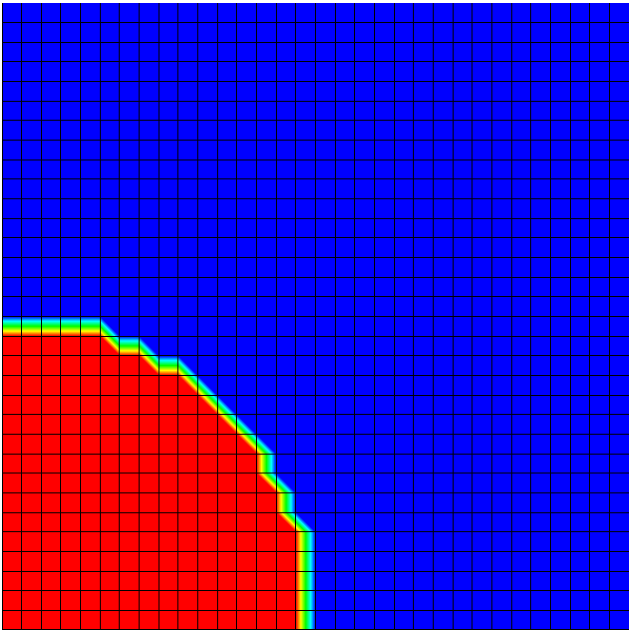
(a) initial temperature and mesh

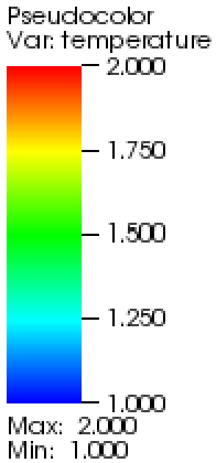
(b) temperature legend

Fig. 1: Initial temperature distribution, mesh, and legend

6.1.1 DEIM versus DEIM-SNS

The DEIM and DEIM-SNS approaches are compared numerically. For this parabolic problem, the DEIM and DEIM-SNS approach tries to reproduce the solution of the corresponding high fidelity model with the same problem parameter settings. For a parametric case, where the DEIM and DEIM-SNS approaches are trained with a number of sample points in a parameter space and are used to predict the solution of a new parameter point, is considered for the hyperbolic problems in Sections 6.2 and 6.3. Figs. 2, 3 and 4 are generated by setting $T=0.01$ s and $\Delta t=1.0\times 10^{-4}$ s, leading to ${N_{t}}=100$. The relative error and the offline time are plotted as the dimension of nonlinear term basis $n_{f}$ increases. For DEIM-SNS, $\boldsymbol{\Phi}_{f}=\boldsymbol{M}\boldsymbol{\Phi}$ is used if $n_{f}={n_{s}}$ while $\boldsymbol{\Phi}_{f}=\boldsymbol{M}\boldsymbol{\Phi}_{e}$ is used for $n_{f}>{n_{s}}$, where $\boldsymbol{M}$ is a volume matrix.

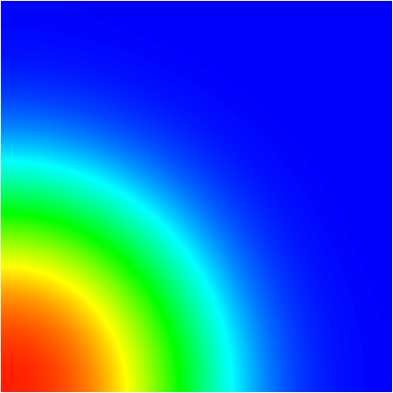
(a) FOM temperature

(b) DEIM temperature

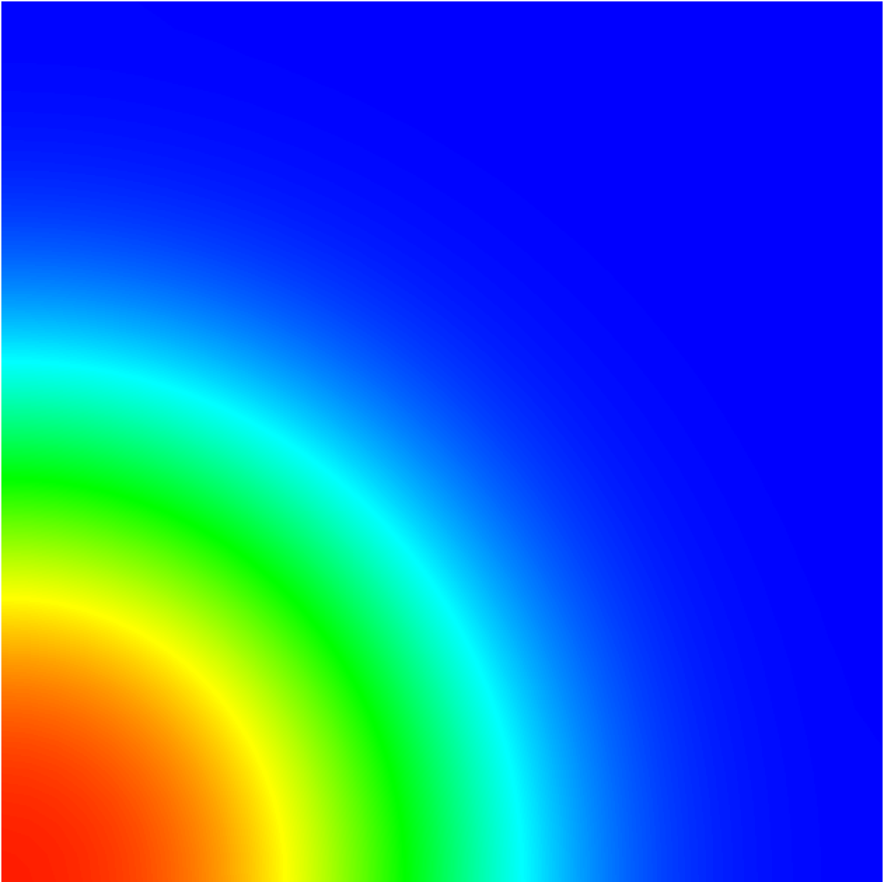
(c) DEIM-SNS temperature

Fig. 2: Temperature distribution using the forward Euler time integrator. For the DEIM and DEIM-SNS approaches, ${n_{s}}=20$ and $n_{r}=20$ are used.

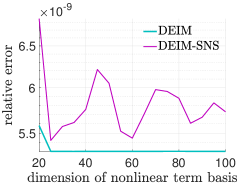
(a) relative error

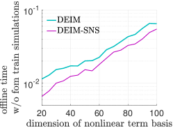
(b) offline time

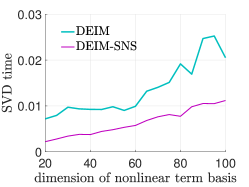
(c) SVD time

Fig. 3: Relative errors and offline time with the forward Euler time integrator, a number of time steps (${N_{t}}=100$).

In Fig. 3(a), the relative errors of both the DEIM and DEIM-SNS approaches are plotted as the dimension of nonlinear term basis increases from 20 to 100 by 5 with the forward Euler time integrator. The figure shows that DEIM-SNS is comparable to DEIM in terms of accuracy. Note that the order of relative errors both with DEIM and DEIM-SNS is $10^{-9}$ for the whole range of the nonlinear term basis dimension considered here. This implies that setting the dimension of the nonlinear term basis $n_{f}$ as small as the dimension of the solution basis ${n_{s}}$ is sufficient to achieve a good accuracy.

Fig. 3(b) shows the offline times required by DEIM and DEIM-SNS. The offline time of the DEIM approach includes the time of two SVDs for the solution and nonlinear term bases construction and the time of constructing sample indices. The offline time of DEIM-SNS includes the time of ‘one’ SVD for the solution basis and nonlinear term basis and the time of constructing sample indices. Because DEIM-SNS requires only one SVD, the offline time of the DEIM-SNS approach is less than the one of the DEIM approach. This fact is shown more clearly in Fig. 3(c) that shows the SVD times only, where DEIM-SNS achieves a speed-up of around two with respect to DEIM. This excludes the time of constructing sample indices from Fig. 3(b).

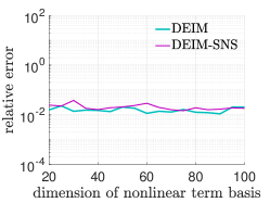
(a) relative error

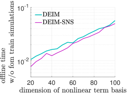
(b) offline time

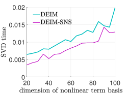
(c) SVD time

Fig. 4: Relative errors and offline time with the backward Euler time integrator, a number of time steps (${N_{t}}=100$).

In Fig. 4(a), the relative errors of both the DEIM and DEIM-SNS approaches are plotted as the dimension of the nonlinear term basis increases from 20 to 100 by 5 with the backward Euler time integrator. The figure shows that the DEIM-SNS approach is comparable to the DEIM approach in terms of accuracy. The order of relative errors of both DEIM and DEIM-SNS is $10^{-2}$ for the whole range of the nonlinear term basis dimensions considered here.

Fig. 4(b) shows the offline time required by DEIM and DEIM-SNS. The offline time of the DEIM approach includes the time of two SVDs for the solution and nonlinear term bases construction and the time of constructing sample indices. The offline time of the DEIM-SNS approach includes the time of ‘one’ SVD for the solution and nonlinear term bases construction and the time of constructing sample indices. Because DEIM-SNS requires only one SVD, the offline time of DEIM-SNS is less than the one of DEIM. This fact is shown more clearly in Fig. 4(c) that shows the SVD times only. This excludes the time of constructing sample indices from Fig. 4(b).

6.2 Parameterized 1D Burgers’ equation

We first consider the parameterized inviscid Burgers’ equation described in Ref. [31], which corresponds to the following initial boundary value problem for $x\in[0,1]$ m and $t\in[0,T]$ with $T=0.5$ s:

(6.5) $$\begin{split}\frac{\partial w(x,t;\mu)}{\partial t}+\frac{\partial f(w(x,t;\mu))}{\partial x}&=0.02e^{\mu_{2}x},\quad\forall x\in[0,1],\quad\forall t\in[0,T]\\ w(0,t;\boldsymbol{\mu})&=\mu_{1},\quad\forall t\in[0,T]\\ w(x,0)&=1,\quad\forall x\in[0,1]\end{split}$$

where $w:[0,1]\times[0,T]\times\mathcal{D}\rightarrow\mathbb{R}$ is a conserved quantity and the $n_{\mu}=2$ parameters comprise the left boundary value and source-term coefficient with $\boldsymbol{\mu}\equiv(\mu_{1},\mu_{2})\in\mathcal{D}=[1.2,1.5]\times[0.02,0.025]$.

After applying Godunov’s scheme for spatial discretization, Eqs. (6.5) lead to a parameterized initial-value ODE problem consistent with Eq. (2.1) with $\boldsymbol{M}$ being an identity matrix. For this problem, all ROMs employ a training set $\mathcal{D}_{\text{train}}=\{1.2,1.3,1.4,1.5\}\times\{0.02,0.025\}$ such that $n_{\text{train}}=8$ at which the FOM is solved. Then, the target parameter, $\boldsymbol{\mu}=(1.45,0.0201)$, is pursued.

6.2.1 GNAT-SNS versus GNAT

For the spatial ROMs the domain is discretized with $1\,000$ control volumes, for $N_{s}=1\,000$ spatial degrees of freedom. We employ ${N_{t}}=2\,000$, leading to a uniform time step of $\Delta t=2.5\times 10^{-4}$. The solution basis dimension of ${n_{s}}=100$ is used. The relative error and the offline time are plotted as the dimension of nonlinear residual term basis $n_{r}$ increases. For the GNAT-SNS method, $\boldsymbol{\Phi}_{r}=\boldsymbol{M}\boldsymbol{\Phi}$ is set if $n_{r}={n_{s}}$, while $\boldsymbol{\Phi}_{r}=\boldsymbol{M}\boldsymbol{\Phi}_{e}$ is set for $n_{r}>{n_{s}}$.

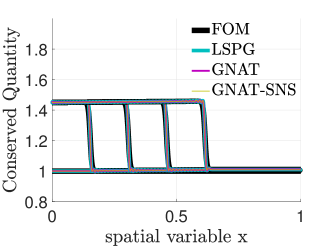
(a) forward Euler time integrator

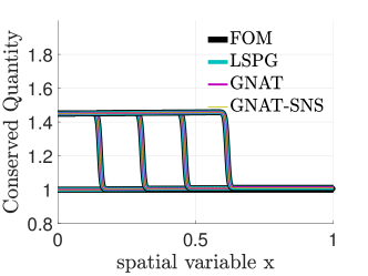
(b) backward Euler time integrator

Fig. 5: Solution snapshots at $t\in\{0,0.125,0.25,0.375,0.5\}$, $n_{r}=100$, $n_{z}=300$

Figs. 5 compare the solution snapshots of several methods: the LSPG, GNAT, and GNAT-SNS methods with the FOM solution snapshots. Fig. 5(a) is generated with the forward Euler time integrator, while Fig. 5(b) is generated with the backward Euler time integrator. All the methods are able to generate almost the same solutions as the FOM solutions.

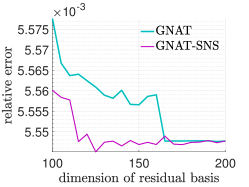
(a) forward Euler

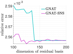
(b) Adams–Bashforth

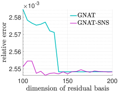
(c) midpoint Runge–Kutta

Fig. 6: Relative errors with respect to FOM solution for explicit time integrators

In Figs. 6, the relative errors of both the GNAT and GNAT-SNS methods are plotted as the dimension of the residual basis ($n_{r}$) increases from 100 to 200 by 5 with a fixed number of sample indices, $n_{z}=300$, with the three different explicit time integrators: the forward Euler, the Adams–Bashforth, and the midpoint Runge–Kutta time integrators. The figures show that the GNAT-SNS method is comparable to the GNAT method in terms of accuracy; the order of relative errors are $10^{-3}$ for the whole range of the residual basis dimensions considered here.

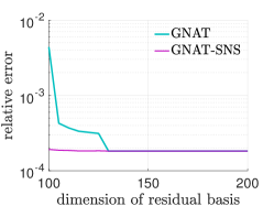
(a) backward Euler

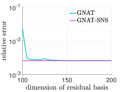
(b) Adams–Moulton

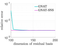
(c) backward differentiation formula

Fig. 7: Relative errors with respect to FOM solution for implicit time integrators

In Figs. 7, the relative errors of both the GNAT and GNAT-SNS methods are plotted as the dimension of residual basis ($n_{r}$) increases from 100 to 200 by 5 with a fixed number of sample indices, $n_{z}=300$, with the three different implicit time integrators: the backward Euler, the Adams–Moulton, and the BDF time integrators. The figures show that the GNAT-SNS method produces results with better accuracy than the GNAT method when the residual basis dimensions are between 100 and 120 (i.e., $n_{r}\approx{n_{s}}$). In fact, the GNAT-SNS achieves an accuracy as good as the LSPG can achieve. We are not sure why this is so at this time, but it would be interesting to investigate the cause of it in the future work.

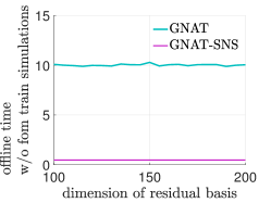
(a) forward Euler

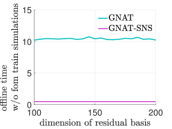
(b) Adams–Bashforth

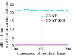
(c) midpoint Runge–Kutta

Fig. 8: Offline time for explicit time integrators

Figs. 8 show the offline time of the GNAT and GNAT-SNS methods for the three different explicit time integrators. The offline time of the GNAT method includes the time of two SVDs for the solution and residual bases construction, the time of the training LSPG simulations for collecting residual snapshots, and the time of constructing sample indices. The offline time of the GNAT-SNS method includes the time of ‘one’ SVD for the solution and residual bases and the time of constructing sample indices. Because the GNAT-SNS method does not need to solve the training LSPG simulations for collecting residual snapshots and it requires only one SVD, the offline time of the GNAT-SNS is less than the one of the GNAT method. Here, we obtain the offline computational time speed-up, a factor of 20 to 40 with the SNS methods.

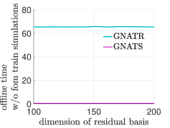
(a) backward Euler

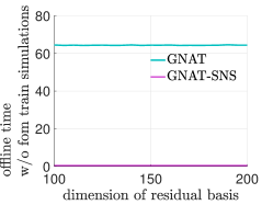
(b) Adams–Moulton

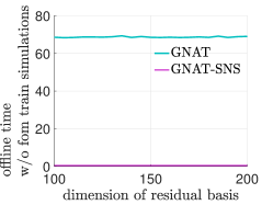
(c) backward differentiation formula

Fig. 9: Offline time for implicit time integrators

Figs. 9 show the offline time of the GNAT and GNAT-SNS methods for the three different implicit time integrators. Because the GNAT-SNS method does not need to solve the training LSPG simulations for collecting residual snapshots and it requires only one SVD, the offline time of the GNAT-SNS method is less than the one of the GNAT method. Here, we obtain the offline computational time speed-up, an order of 100 with the SNS methods.

6.2.2 ST-GNAT-SNS versus ST-GNAT

For the space–time ROMs, the domain is discretized with $100$ control volumes, for $N_{s}=100$ spatial degrees of freedom. The time discretization used in the space–time ROMs is the backward Euler time integrator. We employ ${N_{t}}=2\,000$, leading to a uniform time step of $\Delta t=2.5\times 10^{-4}$ s. The description for the various ways of collecting the space–time residual snapshots are shown in Sections 3.3 and 4.3. We use ST-LSPG ROM training iterations to collect the ST-GNAT residual basis snapshots. The relative error and the offline time are plotted as the dimension of nonlinear residual term basis $n_{r}$ increases. For the ST-GNAT-SNS method, we set ${\bar{\boldsymbol{\Phi}}}_{r}=\bar{\boldsymbol{\Phi}}$ if ${n_{st}}=n_{r}$, while ${\bar{\boldsymbol{\Phi}}}_{r}=\bar{\boldsymbol{\Phi}}_{e}$ is used if ${n_{st}}<n_{r}$.

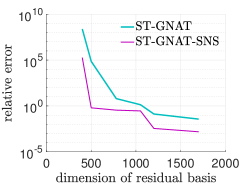
(a) ST-HOSVD

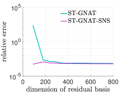
(b) LL1

Fig. 10: Relative errors of the space–time ROMs for solving Burgers’ equation

Figs. 10 show the relative error for the two different space–time basis generation methods, namely two different tensor decompositions: ST-HOSVD and LL1. For each case, the dimension of residual basis $n_{r}$ varies. For the ST-HOSVD, we use ${n_{st}}=400$ and $n_{r}\in\{400$, $500$, $780$, $1\,050$, $1\,200$, $1\,700\}$. For the LL1, we use ${n_{st}}=90$ and $n_{r}\in\{90$, $180$, $240$, $280$, $350$, $400$, $480$, $540$, $630$, $700$, $800\}$. For all the cases, the ST-GNAT-SNS method is comparable to the ST-GNAT method.

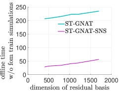
(a) ST-HOSVD

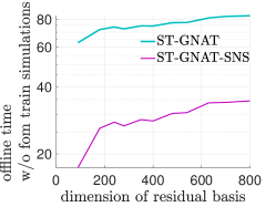
(b) LL1

Fig. 11: Offline time of the space–time ROMs for solving Burgers’ equation

Figs. 11 show the offline time of the ST-GNAT and ST-GNAT-SNS methods. The offline time of the ST-GNAT method includes the time of two tensor decompositions (e.g., ST-HOSVD or LL1) for the solution and residual bases construction, the time of the training ST-LSPG simulations for collecting residual snapshots, and the time of constructing sample indices. The offline time of the ST-GNAT-SNS method includes the time of ‘one’ tensor decomposition for the solution and residual bases and the time of constructing sample indices. Because the ST-GNAT-SNS does not need to solve the training ST-LSPG simulations for collecting residual snapshots and it only requires one tensor decomposition, the offline time of the ST-GNAT-SNS method is less than the one of the ST-GNAT method. Here, we obtain the offline computational time speed-up, a factor of three to seven with the SNS methods.

6.3 Parameterized quasi-1D Euler equation

We now consider a parameterized quasi-1D Euler equation associated with modeling inviscid compressible flow in a one-dimensional converging–diverging nozzle with a continuously varying cross-sectional area [29, Chapter 13]; Figure 12 depicts the problem geometry.

Fig. 12: Quasi-1D Euler. Schematic figures of converging-diverging nozzle.

The governing system of nonlinear partial differential equations is

(6.6) $$\frac{\partial\boldsymbol{w}}{\partial t}+\frac{1}{A}\frac{\partial(\boldsymbol{f}(\boldsymbol{w})A)}{\partial x}=\boldsymbol{q}(\boldsymbol{w}),\quad\forall x\in[0,1]\ \text{m},\quad\forall t\in[0,T],$$

where $T=0.6$ s and

(6.7) $$\boldsymbol{w}=\begin{bmatrix}\rho\\ \rho u\\ e\end{bmatrix},\quad\boldsymbol{f}(\boldsymbol{w})=\begin{bmatrix}\rho u\\ \rho u^{2}+p\\ (e+p)u\end{bmatrix},\quad\boldsymbol{q}(\boldsymbol{w})=\begin{bmatrix}0\\ \frac{p}{A}\frac{\partial A}{\partial x}\\ 0\end{bmatrix},\quad p=(\gamma-1)\rho\epsilon,\quad\epsilon=\frac{e}{\rho}-\frac{u^{2}}{2},\quad A=A(x).$$

Here, $\rho$ denotes density, $u$ denotes velocity, $p$ denotes pressure, $\epsilon$ denotes potential energy per unit mass, $e$ denotes total energy density, $\gamma$ denotes the specific heat ratio, and $A$ denotes the converging–diverging nozzle cross-sectional area. We employ a specific heat ratio of $\gamma=1.3$, a specific gas constant of $R=355.4$ $\text{m}^{2}/\text{s}^{2}/\text{K}$, a total temperature of $T_{t}=300$ K, and a total pressure of $p_{t}=10^{6}$ $\text{N}/\text{m}^{2}$. The cross-sectional area $A(x)$ is determined by a cubic spline interpolation over the points $(x,A(x))\in\{(0,0.2)$, $(0.25,0.173)$, $(0.5,0.17)$, $(0.75,0.173)$, $(1,0.2)\}$, which results in

(6.8) $$A(x)=\left\{\begin{array}[]{ll}-0.288x^{3}+0.4080x^{2}-0.1920x+0.2,&x\in[0,0.25)\ \text{m}\\ -0.288(x-0.25)^{3}+0.1920(x-0.25)^{2}-0.0420(x-0.25)+0.1730,&x\in[0.25,0.5)\ \text{m}\\ 0.288(x-0.5)^{3}-0.0240(x-0.5)^{2}+0.17,&x\in[0.5,0.75)\ \text{m}\\ 0.288(x-0.75)^{3}+0.1920(x-0.75)^{2}+0.0420(x-0.75)+0.1730,&x\in[0.75,1]\ \text{m}.\end{array}\right.$$

A perfect gas is assumed that obeys the ideal gas law (i.e., $p=\rho RT$). The initial flow field is created in several steps. First, the following isentropic relations are used to generate a zero pressure-gradient flow field:

(6.9) $$\begin{split}M(x)&=\frac{M_{m}A_{m}}{A(x)}\left(\frac{1+\frac{\gamma-1}{2}M(x)^{2}}{1+\frac{\gamma-1}{2}M_{m}^{2}}\right)^{\frac{\gamma+1}{2(\gamma-1)}},\quad p(x)=p_{t}\left(1+\frac{\gamma-1}{2}M(x)^{2}\right)^{\frac{-\gamma}{\gamma-1}}\\ T(x)&=T_{t}\left(1+\frac{\gamma-1}{2}M(x)^{2}\right)^{-1},\quad\rho(x)=\frac{p(x)}{RT(x)},\quad c(x)=\sqrt{\gamma\frac{p(x)}{\rho(x)}},\quad u(x)=M(x)c(x),\end{split}$$

where a subscript $m$ indicates the flow quantity at $x=0.5$ m, and $M$ denotes the Mach number. Then, a shock is placed at $x=0.85$ m of the flow field. The jump relations for a stationary shock and the perfect gas equation of state are used to derive the velocity across the shock $u_{2}$, which satisfies the quadratic equation

(6.10) $$\left(\frac{1}{2}-\frac{\gamma}{\gamma-1}\right)u_{2}^{2}+\frac{\gamma}{\gamma-1}\frac{n}{m}u_{2}-h=0.$$

Here, $m:=\rho_{2}u_{2}=\rho_{1}u_{1}$, $n:=\rho_{2}u_{2}^{2}+p_{2}=\rho_{1}u_{1}^{2}+p_{1}$, $h:=(e_{2}+p_{2})/\rho_{2}=(e_{1}+p_{1})/\rho_{1}$, and subscripts $1$ and $2$ denote a flow quantity to the left and to the right of the shock, respectively. The solution $u_{2}$ is employed to Eq. (6.10) that leads to a discontinuity (i.e., shock). Finally, the exit pressure is increased to a factor $P_{\text{exit}}$ of its original value in order to generate transient dynamics.

Applying a finite-volume spatial discretization with 50 equally spaced control volumes and fully implicit boundary conditions leads to a parameterized system of nonlinear ODEs consistent with Eq. (2.1) with $N_{s}=150$ spatial degrees of freedom. The Roe flux difference vector splitting method is used to compute the flux at each intercell face [29, Chapter 9]. For time discretization, we apply the backward Euler scheme and a uniform time step of $\Delta t=0.001$ s, leading to ${N_{t}}=600$.

For this problem, we use the following two parameters: the pressure factor $\mu_{1}=P_{\text{exit}}$ and the Mach number at the middle of the nozzle $\mu_{2}=M_{m}$. All ROMs employ a training set at which the FOM is solved of $\mathcal{D}_{\text{train}}=\{1.7+0.01i\}_{i=0}^{3}\times\{1.7,1.72\}$ such that $n_{\text{train}}=8$. Then the target parameter, $\boldsymbol{\mu}=(1.7225,1.705)$, is pursued.

6.3.1 GNAT-SNS versus GNAT

The solution basis dimension of ${n_{s}}=30$ is used. The relative error and the offline time are plotted as the dimension of nonlinear residual term basis $n_{r}$ increases. For the GNAT-SNS method, $\boldsymbol{\Phi}_{r}=\boldsymbol{M}\boldsymbol{\Phi}$ is used if $n_{r}={n_{s}}$, while $\boldsymbol{\Phi}_{r}=\boldsymbol{M}\boldsymbol{\Phi}_{e}$ is used if $n_{r}>{n_{s}}$.

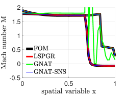
(a) $n_{r}=30$

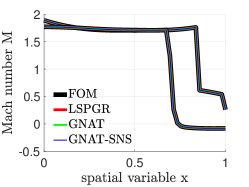
(b) $n_{r}=60$

Fig. 13: Solution snapshots at $t\in\{0,0.6\}$, $n_{z}=90$ with the backward Euler time integrator.

Figs. 13 compare the solution snapshots of several methods: the LSPG, GNAT, and GNAT-SNS methods with the FOM solution snapshots. Fig. 13(a) is generated with $n_{r}=30$ and $n_{z}=90$, while Fig. 13(b) is generated with $n_{r}=60$ and $n_{z}=90$. All the methods are able to generate almost the same solutions as the FOM solutions except for the GNAT method with ${n_{s}}=n_{r}=30$. Surprisingly, the GNAT-SNS method does not suffer when ${n_{s}}=n_{r}$ as shown in Figs. 7 of the Burgers’ example. Again, we do not know why the GNAT-SNS the achieve an accuracy as good as the the one of the LSPG method in this particular example.

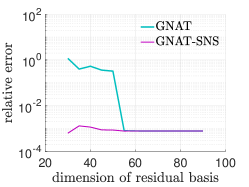
(a) relative error

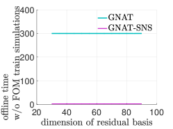
(b) offline time

Fig. 14: Relative errors and offline time with the backward Euler time integrator

In Fig. 14(a), the relative errors of both the GNAT and GNAT-SNS methods are plotted as the dimension of residual basis increases from 30 to 90 by 5 with a fixed number of sample indices, 90. The figures show that the GNAT-SNS method is comparable to the GNAT method in terms of accuracy; the order of relative errors of the GNAT-SNS method is $10^{-3}$ for the whole range of the residual basis dimensions considered here. On the other hand, the relative errors of the GNAT method are bigger than the ones of the GNAT-SNS method when the residual basis dimensions are between 30 and 55. Fig. 14(b) shows the offline time of the GNAT and GNAT-SNS methods. The offline time of the GNAT method includes the time of two SVDs for the solution and residual bases construction, the time of the training LSPG simulations for collecting residual snapshots, and the time of constructing sample indices. The offline time of the GNAT-SNS method includes the time of ‘one’ SVD for the solution and residual bases construction and the time of constructing sample indices. Because the GNAT-SNS method does not need to solve the training LSPG simulations for collecting residual snapshots and it requires only one SVD, the offline time of the GNAT-SNS method is less than the one of the GNAT method. Here, we get a factor of 130 speed-up in the offline computational time with the GNAT-SNS method.

6.3.2 ST-GNAT-SNS versus ST-GNAT

The relative error and the offline time of both the ST-GNAT and ST-GNAT-SNS methods are plotted as the dimension of nonlinear residual term basis $n_{r}$ increases. For the ST-GNAT-SNS method, we set ${\bar{\boldsymbol{\Phi}}}_{r}=\bar{\boldsymbol{\Phi}}$ if ${n_{st}}=n_{r}$, while ${\bar{\boldsymbol{\Phi}}}_{r}=\bar{\boldsymbol{\Phi}}_{e}$ is used if ${n_{st}}<n_{r}$.

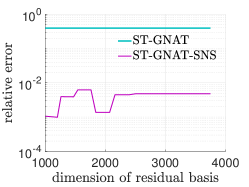
(a) ST-HOSVD

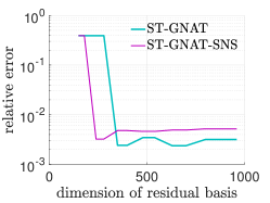
(b) LL1

Fig. 15: Relative errors and offline time with the backward Euler time integrator

In Figs. 15, the relative errors of both the ST-GNAT and ST-GNAT-SNS methods are shown for two different tensor decompositions: ST-HOSVD and LL1. For the ST-HOSVD, we use ${n_{st}}=1\,000$ and $n_{r}\in\{1\,000$, $1\,200$, $1\,260$, $1\,470$, $1\,540$, $1\,760$, $1\,840$, $2\,070$, $2\,160$, $2\,400$, $2\,500$, $3\,000$, $3\,500$, $3\,750\}$. For the LL1 decomposition, we use ${n_{st}}=150$ and $n_{r}\in\{150$, $180$, $240$, $280$, $350$, $400$, $480$, $540$, $630$, $700$, $800$, $960\}$. For the ST-HOSVD, the ST-GNAT-SNS method achieves two orders of magnitude better accuracy than the ST-GNAT method. For the LL1 decomposition, the ST-GNAT-SNS method generate results as good as the ST-GNAT method.

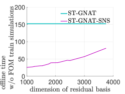
(a) ST-HOSVD

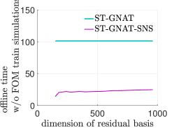
(b) LL1

Fig. 16: Offline time of the space–time ROMs for solving Euler equation

Figs. 16 show the offline time of the ST-GNAT and ST-GNAT-SNS methods. The offline time of the ST-GNAT method includes the time of two tensor decompositions (e.g., ST-HOSVD or LL1) for the solution and residual bases construction, the time of the training ST-LSPG simulations for collecting residual snapshots, and the time of constructing sample indices. The offline time of the ST-GNAT-SNS method includes the time of ‘one’ tensor decomposition for the solution and residual bases construction and the time of constructing sample indices. Because the ST-GNAT-SNS does not need to solve the training ST-LSPG simulations for collecting residual snapshots and it only requires one tensor decomposition, the offline time of the ST-GNAT-SNS method is less than the one of the ST-GNAT method. Here, we get a factor of six to seven speed-up in the offline computational time with the SNS methods.

7 Conclusion

We have introduced a new way of constructing nonlinear term basis using solution snapshots to construct a projection-based reduced order model for solving a nonlinear dynamical system of equations, which is characterized by an ordinary differential equation. Our proposed method, the SNS method, is theoretically justified by the conforming subspace condition and the subspace inclusion relation.

The two main advantages of the SNS method over the traditional hyper-reduction methods considered here are 1) the avoidance of collecting nonlinear term snapshots and 2) the avoidance of the second data compression process. These advantages result in the offline computational time reduction, which is demonstrated in numerical experiments. The benefits of the SNS method are more vivid when it is compared with GNAT and ST-GNAT than DEIM because the GNAT and ST-GNAT methods require collecting the nonlinear residual snapshots from the corrsponding LSPG and ST-LSPG simulations. These benefits are also demonstrated in numerical experiments, where parametric GNAT and ST-GNAT are compared with the SNS methods. There, we have shown that a considerable speed-up in the offline computational time is achieved by the SNS methods. Also, the error analysis contributes to the theoretical insight about the effects of the volume matrix $\boldsymbol{M}$ on the oblique projection of the SNS method, revealing that the conditioner number of $\boldsymbol{M}$ can affect the error due to the oblique projection. This issue can be addressed by pre-orthogonalization process.

In numerical experiments, we observe that the SNS methods produce a more accurate solution than the DEIM, GNAT, and ST-GNAT methods with a smaller number of nonlinear term basis vectors, especially for the GNAT-SNS method. The reason for this attractive feature of the GNAT-SNS method will be investigated in future work.

Appendix A Subspace inclusion relation

The forward and backward Euler time integrators and their corresponding subspace inclusion relations are shown in Section 2. Here, we show several other time integrators and corresponding subspace inclusion relation between the subspace spanned by the nonlinear term snapshots and the subspace spanned by the solution snapshots.

A.1 The Adams–Bashforth methods

The second order Adams–Bashforth (AB) method numerically solves Eq. (2.1), by solving the following nonlinear system of equations for $\boldsymbol{x}_{n}$ at $n$-th time step:

(A.1) $$\boldsymbol{M}\boldsymbol{x}_{n}-\boldsymbol{M}\boldsymbol{x}_{n-1}=\Delta t\left(\frac{3}{2}\boldsymbol{f}_{n-1}-\frac{1}{2}\boldsymbol{f}_{n-2}\right),$$

Eq. (A.1) implies the following subspace inclusions:

(A.2) $$\mathrm{span}\{\boldsymbol{f}_{n-2},\boldsymbol{f}_{n-1}\}\subseteq\mathrm{span}\{\boldsymbol{M}\boldsymbol{x}_{n-1},\boldsymbol{M}\boldsymbol{x}_{n}\}.$$

By induction, we conclude that

(A.3) $$\mathrm{span}\{\boldsymbol{f}_{0},\dots,\boldsymbol{f}_{{N_{t}}-1}\}\subseteq\mathrm{span}\{\boldsymbol{M}\boldsymbol{x}_{0},\ldots,\boldsymbol{M}\boldsymbol{x}_{{N_{t}}}\},$$

which shows that the span of nonlinear term snapshots is a subspace of the span of $\boldsymbol{M}$-scaled solution snapshots. The residual function of the second AB method is defined as

(A.4) $$\begin{split}\boldsymbol{r}^{n}_{\mathrm{AB}}(\boldsymbol{x}_{n};\boldsymbol{x}_{n-1},\boldsymbol{\mu})&:=\boldsymbol{M}(\boldsymbol{x}_{n}-\boldsymbol{x}_{n-1})-\Delta t\left(\frac{3}{2}\boldsymbol{f}_{n-1}-\frac{1}{2}\boldsymbol{f}_{n-2}\right).\end{split}$$

A.2 The Adams–Moulton methods

The second order Adams–Moulton (AM) method numerically solves Eq. (2.1), by solving the following nonlinear system of equations for $\boldsymbol{x}_{n}$ at $n$-th time step:

(A.5) $$\boldsymbol{M}\boldsymbol{x}_{n}-\boldsymbol{M}\boldsymbol{x}_{n-1}=\frac{1}{2}\Delta t(\boldsymbol{f}_{n}+\boldsymbol{f}_{n-1}),$$

Eq. (A.5) implies the following subspace inclusions:

(A.6) $$\mathrm{span}\{\boldsymbol{f}_{n-1},\boldsymbol{f}_{n}\}\subseteq\mathrm{span}\{\boldsymbol{M}\boldsymbol{x}_{n-1},\boldsymbol{M}\boldsymbol{x}_{n}\}.$$

By induction, we conclude that

(A.7) $$\mathrm{span}\{\boldsymbol{f}_{0},\dots,\boldsymbol{f}_{{N_{t}}}\}\subseteq\mathrm{span}\{\boldsymbol{M}\boldsymbol{x}_{0},\ldots,\boldsymbol{M}\boldsymbol{x}_{{N_{t}}}\},$$

which shows that the span of nonlinear term snapshots is a subspace of the span of $\boldsymbol{M}$-scaled solution snapshots. The residual function of the second AM method is defined as

(A.8) $$\begin{split}\boldsymbol{r}^{n}_{\mathrm{AM}}(\boldsymbol{x}_{n};\boldsymbol{x}_{n-1},\boldsymbol{\mu})&:=\boldsymbol{M}(\boldsymbol{x}_{n}-\boldsymbol{x}_{n-1})-\Delta t\frac{1}{2}(\boldsymbol{f}_{n}+\boldsymbol{f}_{n-1}).\end{split}$$

A.3 The backward differentiation formulas

The 2-step BDF numerically solves Eq. (2.1), by solving the following nonlinear system of equations for $\boldsymbol{x}_{n}$ at n-th time step:

(A.9) $$\boldsymbol{M}\boldsymbol{x}_{n}-\frac{4}{3}\boldsymbol{M}\boldsymbol{x}_{n-1}+\frac{1}{3}\boldsymbol{M}\boldsymbol{x}_{n-2}=\frac{2}{3}\Delta t\boldsymbol{f}_{n},$$

Eq. (A.9) implies the following subspace inclusions:

(A.10) $$\mathrm{span}\{\boldsymbol{f}_{n}\}\subseteq\mathrm{span}\{\boldsymbol{M}\boldsymbol{x}_{n-2},\boldsymbol{M}\boldsymbol{x}_{n-1},\boldsymbol{M}\boldsymbol{x}_{n}\}.$$

By induction, we conclude that

(A.11) $$\mathrm{span}\{\boldsymbol{f}_{1},\dots,\boldsymbol{f}_{{N_{t}}-1}\}\subseteq\mathrm{span}\{\boldsymbol{M}\boldsymbol{x}_{0},\ldots,\boldsymbol{M}\boldsymbol{x}_{{N_{t}}}\},$$

which shows that the span of nonlinear term snapshots is a subspace of the span of $\boldsymbol{M}$-scaled solution snapshots. The residual function of the two-step BDF method is defined as

(A.12) $$\begin{split}\boldsymbol{r}^{n}_{\mathrm{BDF}}(\boldsymbol{x}_{n};\boldsymbol{x}_{n-1},\boldsymbol{x}_{n-2},\boldsymbol{\mu})&:=\boldsymbol{M}(\boldsymbol{x}_{n}-\frac{4}{3}\boldsymbol{x}_{n-1}+\frac{1}{3}\boldsymbol{x}_{n-2})-\frac{2}{3}\Delta t\boldsymbol{f}_{n}.\end{split}$$

A.4 The midpoint Runge–Kutta method

The midpoint method, a $2$-stage Runge–Kutta method, takes the following two stages to advance at n-th time step of Eq. (2.1):

(A.13) $$\boldsymbol{M}\boldsymbol{x}_{n-\frac{1}{2}} =\boldsymbol{M}\boldsymbol{x}_{n-1}+\frac{\Delta t}{2}\boldsymbol{f}_{n-1}$$

$$\boldsymbol{M}\boldsymbol{x}_{n} =\boldsymbol{M}\boldsymbol{x}_{n-1}+\Delta t\boldsymbol{f}_{n-\frac{1}{2}}.$$

These lead to the following two subspace inclusion relations:

(A.14) $$\mathrm{span}\{\boldsymbol{f}_{n-1}\} \subseteq\mathrm{span}\{\boldsymbol{M}\boldsymbol{x}_{n-1},\boldsymbol{M}\boldsymbol{x}_{n-\frac{1}{2}}\}$$

$$\mathrm{span}\{\boldsymbol{f}_{n-\frac{1}{2}}\} \subseteq\mathrm{span}\{\boldsymbol{M}\boldsymbol{x}_{n-1},\boldsymbol{M}\boldsymbol{x}_{n}\}.$$

These in turn lead to the following subspace inclusion relation:

(A.15) $$\mathrm{span}\{\boldsymbol{f}_{n-1},\boldsymbol{f}_{n-\frac{1}{2}}\}\subseteq\mathrm{span}\{\boldsymbol{M}\boldsymbol{x}_{n-1},\boldsymbol{M}\boldsymbol{x}_{n-\frac{1}{2}},\boldsymbol{M}\boldsymbol{x}_{n}\}.$$

By induction, we conclude that

(A.16) $$\mathrm{span}\{\boldsymbol{f}_{0},\boldsymbol{f}_{\frac{1}{2}},\ldots,\boldsymbol{f}_{{N_{t}}-1},\boldsymbol{f}_{{N_{t}}-\frac{1}{2}}\}\subseteq\mathrm{span}\{\boldsymbol{M}\boldsymbol{x}_{n-1},\boldsymbol{M}\boldsymbol{x}_{n-\frac{1}{2}},\boldsymbol{M}\boldsymbol{x}_{n},\ldots,\boldsymbol{M}\boldsymbol{x}_{{N_{t}}-1},\boldsymbol{M}\boldsymbol{x}_{{N_{t}}-\frac{1}{2}},\boldsymbol{M}\boldsymbol{x}_{{N_{t}}}\}.$$

References

• [1] BLAST: High-order finite element hydrodynamics. https://computation.llnl.gov/projects/blast/icf-like-implosion.
• [2] MFEM: Modular finite element methods library. mfem.org.
• [3] Steven S An, Theodore Kim, and Doug L James. Optimizing cubature for efficient integration of subspace deformations. ACM transactions on graphics (TOG), 27(5):165, 2008.
• [4] Robert W Anderson, Veselin A Dobrev, Tzanio V Kolev, Robert N Rieben, and Vladimir Z Tomov. High-order multi-material ale hydrodynamics. SIAM Journal on Scientific Computing, 40(1):B32–B58, 2018.
• [5] Patricia Astrid, Siep Weiland, Karen Willcox, and Ton Backx. Missing point estimation in models described by proper orthogonal decomposition. IEEE Transactions on Automatic Control, 53(10):2237–2251, 2008.
• [6] Maxime Barrault, Yvon Maday, Ngoc Cuong Nguyen, and Anthony T Patera. An ‘empirical interpolation’method: application to efficient reduced-basis discretization of partial differential equations. Comptes Rendus Mathematique, 339(9):667–672, 2004.
• [7] Gal Berkooz, Philip Holmes, and John L Lumley. The proper orthogonal decomposition in the analysis of turbulent flows. Annual review of fluid mechanics, 25(1):539–575, 1993.
• [8] Alfredo Buttari, Julien Langou, Jakub Kurzak, and Jack Dongarra. Parallel tiled qr factorization for multicore architectures. Concurrency and Computation: Practice and Experience, 20(13):1573–1590, 2008.
• [9] Kevin Carlberg, Matthew Barone, and Harbir Antil. Galerkin v. least-squares petrov–galerkin projection in nonlinear model reduction. Journal of Computational Physics, 330:693–734, 2017.
• [10] Kevin Carlberg, Charbel Bou-Mosleh, and Charbel Farhat. Efficient non-linear model reduction via a least-squares petrov–galerkin projection and compressive tensor approximations. International Journal for Numerical Methods in Engineering, 86(2):155–181, 2011.
• [11] Kevin Carlberg, Charbel Farhat, Julien Cortial, and David Amsallem. The gnat method for nonlinear model reduction: effective implementation and application to computational fluid dynamics and turbulent flows. Journal of Computational Physics, 242:623–647, 2013.
• [12] Saifon Chaturantabut and Danny C Sorensen. Nonlinear model reduction via discrete empirical interpolation. SIAM Journal on Scientific Computing, 32(5):2737–2764, 2010.
• [13] Youngsoo Choi and Kevin Carlberg. Space–time least-squares petrov–galerkin projection for nonlinear model reduction. SIAM Journal on Scientific Computing, 41(1):A26–A58, 2019.
• [14] Lieven De Lathauwer. Blind separation of exponential polynomials and the decomposition of a tensor in rank-(l_r,l_r,1) terms. SIAM Journal on Matrix Analysis and Applications, 32(4):1451–1474, 2011.
• [15] Zlatko Drmac and Serkan Gugercin. A new selection operator for the discrete empirical interpolation method—improved a priori error bound and extensions. SIAM Journal on Scientific Computing, 38(2):A631–A648, 2016.
• [16] Zlatko Drmac and Arvind Krishna Saibaba. The discrete empirical interpolation method: Canonical structure and formulation in weighted inner product spaces. SIAM Journal on Matrix Analysis and Applications, 39(3):1152–1180, 2018.
• [17] Erik Elmroth and Fred Gustavson. High-performance library software for qr factorization. In International Workshop on Applied Parallel Computing, pages 53–63. Springer, 2000.
• [18] Richard Everson and Lawrence Sirovich. Karhunen–loeve procedure for gappy data. JOSA A, 12(8):1657–1664, 1995.
• [19] Charbel Farhat, Philip Avery, Todd Chapman, and Julien Cortial. Dimensional reduction of nonlinear finite element dynamic models with finite rotations and energy-based mesh sampling and weighting for computational efficiency. International Journal for Numerical Methods in Engineering, 98(9):625–662, 2014.
• [20] Charbel Farhat, Todd Chapman, and Philip Avery. Structure-preserving, stability, and accuracy properties of the energy-conserving sampling and weighting method for the hyper reduction of nonlinear finite element dynamic models. International Journal for Numerical Methods in Engineering, 102(5):1077–1110, 2015.
• [21] Martin A Grepl, Yvon Maday, Ngoc C Nguyen, and Anthony T Patera. Efficient reduced-basis treatment of nonaffine and nonlinear partial differential equations. ESAIM: Mathematical Modelling and Numerical Analysis, 41(3):575–605, 2007.
• [22] Ming Gu and Stanley C Eisenstat. Efficient algorithms for computing a strong rank-revealing qr factorization. SIAM Journal on Scientific Computing, 17(4):848–869, 1996.
• [23] Joaquin Alberto Hernandez, Manuel Alejandro Caicedo, and Alex Ferrer. Dimensional hyper-reduction of nonlinear finite element models via empirical cubature. Computer methods in applied mechanics and engineering, 313:687–722, 2017.
• [24] Michael Hinze and Stefan Volkwein. Proper orthogonal decomposition surrogate models for nonlinear dynamical systems: Error estimates and suboptimal control. In Dimension reduction of large-scale systems, pages 261–306. Springer, 2005.
• [25] Harold Hotelling. Analysis of a complex of statistical variables into principal components. Journal of educational psychology, 24(6):417, 1933.
• [26] Saad A Khairallah and Andy Anderson. Mesoscopic simulation model of selective laser melting of stainless steel powder. Journal of Materials Processing Technology, 214(11):2627–2636, 2014.
• [27] Karl Kunisch and Stefan Volkwein. Galerkin proper orthogonal decomposition methods for a general equation in fluid dynamics. SIAM Journal on Numerical analysis, 40(2):492–515, 2002.
• [28] Michel Loeve. Probability Theory. D. Van Nostrand, New York, 1955.
• [29] Robert MacCormack. Numerical computation of compressible viscous flow. Technical report, Lecture notes for AA214b and AA214c, Stanford University, 2007.
• [30] Ngoc C Nguyen and Jaime Peraire. An efficient reduced-order modeling approach for non-linear parametrized partial differential equations. International Journal for Numerical Methods in Engineering, 76(1):27–55, 2008.
• [31] Michał Jerzy Rewieński. A trajectory piecewise-linear approach to model order reduction of nonlinear dynamical systems. PhD thesis, Massachusetts Institute of Technology, Department of Electrical Engineering and Computer Science, 2003.
• [32] David Ryckelynck. A priori hyperreduction method: an adaptive approach. Journal of computational physics, 202(1):346–366, 2005.
• [33] Laurent Sorber, Marc Van Barel, and Lieven De Lathauwer. Optimization-based algorithms for tensor decompositions: Canonical polyadic decomposition, decomposition in rank-(l_r,l_r,1) terms, and a new generalization. SIAM Journal on Optimization, 23(2):695–720, 2013.
• [34] Matthew J Zahr, K Carlberg, D Amsallem, and C Farhat. Comparison of model reduction techniques on high-fidelity linear and nonlinear electrical, mechanical, and biological systems. University of California, Berkeley, 2010.