Neural-Augmented Static Analysis of Android Communication

Abstract.

We address the problem of discovering communication links between applications in the popular Android mobile operating system, an important problem for security and privacy in Android. Any scalable static analysis in this complex setting is bound to produce an excessive amount of false-positives, rendering it impractical. To improve precision, we propose to augment static analysis with a trained neural-network model that estimates the probability that a communication link truly exists. We describe a neural-network architecture that encodes abstractions of communicating objects in two applications and estimates the probability with which a link indeed exists. At the heart of our architecture are type-directed encoders (tde), a general framework for elegantly constructing encoders of a compound data type by recursively composing encoders for its constituent types. We evaluate our approach on a large corpus of Android applications, and demonstrate that it achieves very high accuracy. Further, we conduct thorough interpretability studies to understand the internals of the learned neural networks.

1. Introduction

In Android, the popular mobile operating system, applications can communicate with each other using an Android-specific message-passing system called Inter-Component Communication (icc). Misuse and abuse of icc may lead to several serious security vulnerabilities, including theft of personal data as well as privilege-escalation attacks (Enck et al., 2011; Chin et al., 2011; Zhou and Jiang, 2013; Grace et al., 2012). Indeed, researchers have discovered various such instances (Chin et al., 2011)—a bus application that broadcasts gps location to all other applications, an sms-spying application that is disguised as a tip calculator, amongst others. Thus, it is important to detect inter-component communication: Can component $c$ communicate with component $d$? (We say that $c$ and $d$ have a link.)

With the massive size of Android’s application market and the complexity of the Android ecosystem and its applications, a sound and scalable static analysis for link inference is bound to produce an overwhelmingly large number of false-positive links. Realistically, however, a security engineer needs to manually investigate malicious links, and so we need to carefully prioritize their attention.

To address false positives in this setting, recently Octeau et al. (2016a) presented primo, a hand-crafted probabilistic model that assigns probabilities to icc links inferred by static analysis, thus ordering links by how likely they are to be true positives. We see multiple interrelated problems with primo’s methodology: First, the model is manually crafted; constructing the model is a laborious, error-prone process requiring deep expert domain knowledge in the intricacies of Android applications, the icc system, and the static analysis at hand. Second, the model is specialized; hence, changes in the Android programming framework—which is constantly evolving—or the static analysis may render the model obsolete, requiring a new expert-crafted model.

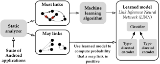
Figure 1. Overview of our approach

Model-Augmented Link Inference

Our high-level goal is:

To automatically construct a probabilistic model that augments static analysis, using minimal domain knowledge.

To achieve this, we view the link-inference problem through the lens of machine learning. We make the observation that we can categorize results of a static analysis into must and may categories: links for which we are sure whether they exist or not (must links), and others for which we are unsure (may links). We then utilize must links to train a machine learning classifier, which we then apply to approximate the likelihood of a may link being a true positive. Figure 1 presents an overview of our proposed approach.

Link-Inference Neural Networks

To enable machine learning in our setting, we propose a custom neural-network architecture targeting the link-inference problem, which we call link-inference neural network (linn). The advantages of using a neural network for this setting—and generally in machine learning—is to automatically extract useful features of link artifacts (specifically, the addressing mechanism in icc). We can train the network to encode the artifacts into real-valued vectors that capture relevant features. This relieves us from the arduous and brittle task of manual feature extraction, which requires (i) expert domain knowledge and (ii) maintenance in case of changes in Android icc or the used static analysis.

The key novelty of linns is what we call a type-directed encoder (tde): a generic framework for constructing neural networks that encode elements of some type $\tau$ into real-valued vectors. We use tdes to encode abstractions of link artifacts produced by static analysis, which are elements of some data type representing an abstract domain. tdes exploit the inherent recursive structure of a data type: We can construct an encoder for values of a compound data type by recursively composing encoders for its constituent types. For instance, if we want to encode elements of the type $\texttt{int}\times\texttt{string}$, then we compose an encoder of int and an encoder of string.

We demonstrate how to construct encoders for a range of types, including lists, sets, product types, and strings, resulting in a generic approach. Our tde framework is parameterized by differentiable functions, which can be instantiated using different neural-network architectures. Depending on how we instantiate our tde framework, we can arrive at different encoders. At one extreme, we can use tdes to simply treat a value of some data type as its serialized value, and use a convolutional (cnn) or recurrent neural network (rnn) to encode it; at the other extreme, we show how tdes can be instantiated as a Tree-lstm (Tai et al., 2015), an advanced architecture that maintains the tree-like structure of a value of a data type. This allows us to systematically experiment with various encodings of abstract states computed by static analysis.

Contributions

We make the following contributions:

• Model-Augmented Link Inference (§3): We formalize and investigate the problem of augmenting a static analysis for Android icc with an automatically learned model that assigns probabilities to inferred links.

• Link-Inference NN Framework (§4): We present a custom neural-network architecture, link-inference neural network (linn), for augmenting a link inference static analysis . At the heart of linns are type-directed encoders (tde), a framework that allows us to construct encoder neural networks for a compound data type by recursively composing encoders of its component types.

• Instantiations & Empirical Evaluation (§5): We implement our approach using TensorFlow (Abadi et al., 2016) and ic3 (Octeau et al., 2016b) and present a thorough evaluation on a large corpus of $10,500$ Android applications from the Google Play Store. We present multiple instantiations of our tdes, ranging in complexity and architecture. Our results demonstrate very high classification accuracy. Significantly, our automated technique outperforms primo, which relied on $6$ to $9$ months of manual model engineering.

• Interpretability Study (§6): To address the problem of opacity of deep learning, we conduct a detailed interpretability investigation to explain the behavior of our models. Our results provide strong evidence that our models learn to mimic the link-resolution logic employed by the Android operating system.

2. Android ICC: Overview & Definitions

We now (i) provide relevant background about Android icc, and (ii) formally define intents, filters, and their static abstractions.

2.1. ICC Overview and Examples

Android applications are conceptually collections of components, with each component designed to perform a specific task, such as display a particular screen to the user or play music files. Applications can leverage the functionality of other applications through the use of a sophisticated message-passing system, generally referred to as Inter-Component Communication (icc). To illustrate, say an application developer desires the ability to dial a phone number. Rather than code that functionality from scratch, the developer can instead send a message requesting that some other application handle the dialing process. Further, such messages are often generic, i.e., not targeted at a specific application. The same communication mechanism is also used to send messages within an application. Consequently, any inter-component or inter-application program analysis must first begin by computing the icc links.

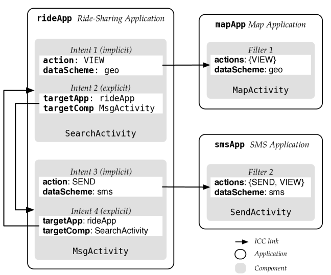
(a) icc example with three applications

⬇

public void sendImplicitIntent() {

Intent intent = new Intent();

intent.setAction("SEND");

msg = ... // contains phone # and msg

intent.setData(msg);

startActivity(intent);}

Code constructing and starting implicit intent

⬇

<intent-filter>

<action android:name="SEND"/>

<action android:name="VIEW"/>

<data android:scheme="sms"/>

<category android:name="DEFAULT"/>

</intent-filter>

Intent filter for a sms component

(b) Intent for sending an sms and associated filter

Figure 2. ICC Example

Intents

Figure 2(a) illustrates a simplified icc example with a ride-sharing application (rideApp) that uses functionality of a map application (mapApp) and an sms-messaging application (smsApp). Each application comprises components (gray boxes), and arrows in the figure represent potential links between components. icc is primarily accomplished using intents. Intents are messages sent between Android components. An intent can be either explicit or implicit. The former specifies the target application and component; the latter merely specifies the functionality it requires from its target.

Consider, for instance, the implicit intent 3 in Figure 2(a); it requests the action SEND (send an sms), which sends sms data. By issuing this intent (Figure 2(b) top), rideApp is able to send a message without having to worry about how this action is performed and by whom.

Intent Filters

Components that wish to receive implicit intents have to declare intent filters (filters for short), which describe the attributes of the intents that they are willing to receive (i.e., subscribe to intents of those types). For instance, filter 2 in Figure 2(a) specifies that smsApp can handle SEND and VIEW actions (Figure 2(b) (bottom) shows the code declaring this filter). Therefore, when the ride-sharing application issues an intent with a SEND action, Android’s intent-resolution process matches it with smsApp, which offers that functionality. Security and privacy issues arise, for instance, when malicious applications are installed that intercept sms messages by declaring that they also handle SEND actions (Chin et al., 2011; Yang et al., 2015; Elish et al., 2015).

2.2. Intents, Filters, and their Abstraction

We now formalize intents and filters. We use ${\Sigma^{*}}$ to denote the set of all strings, and $\omega$ to denote an undefined value (null).

Definition 2.1 (Intents).

An intent $\iota$ is a pair $(\emph{act},\emph{cats})$, where:

• $\emph{act}\in{\Sigma^{*}}\cup\{\omega\}$ is a string defining the action of $\iota$, e.g., the string "SEND" in Figure 2(b) (top), or the value $\omega$.

• $\emph{cats}\in 2^{\Sigma^{*}}$ is a set of strings defining categories, which provide further information of how to run the intent. For instance, "APP_BROWSER" means that the intent should be able to browse the web; If an intent is created without providing categories, cats is instantiated into the singleton set $\{\texttt{"DEFAULT"}\}$.

Practically, intents also contain the issuing component’s name as well as data like a phone number, image, or email. We elide these other fields because, based on our dataset, they provided little information: less than 10% of intents/filters have fields other than actions and categories and even when they have them, the values have few distinct possibilities. It is, however, conceivable that as we investigate more applications, other fields will become important.

Definition 2.2 (Filters).

A filter $f$ is a tuple $(\emph{acts},\emph{cats})$, where:

• $\emph{acts}\in 2^{\Sigma^{*}}$ is a set of strings defining actions a filter can perform.

• $\emph{cats}\in 2^{\Sigma^{*}}$ is a set of category strings (see Definition 2.1).

Like intents, filters also contain more attributes, but, for our purposes, actions and categories are most relevant.

Semantics

We will use $I$ and $F$ to denote the sets of all possible intents and filters. We characterize an Android application $A$ by the (potentially infinite) set of intents $I_{A}\subseteq I$ and filters $F_{A}\subseteq F$ it can create—i.e., the collecting semantics of the application.

Let $Y=\{0,1\}$, indicating whether a link exists (1) or not (0). We use the matching function $\emph{match}:I\times F\rightarrow Y$ to denote an oracle that, given an intent $\iota$ and filter $f$, determines whether $(\iota,f)$ can ever match at runtime—i.e., there is a link between them—following the Android intent-resolution process. We refer to Octeau et al. (2016a) for a formal definition of match.

Example 2.3.

Consider the intent and filter described in Figure 2(b). The intent carries a SEND action, which matches one of the actions specified in the filter. The msg in the intent it has an sms data scheme so that it matches the filter data scheme. As for the category, the Android api startActivity initializes the categories of the intent to the set "DEFAULT". This then matches the filter’s "DEFAULT" category. Thus, the intent and filter of Figure 2(b) match successfully.

Static Analysis

We assume that we have a domain of abstract intents and abstract filters, denoted $I^{\#}$ and $F^{\#}$, respectively. Semantically, each abstract intent $\iota^{\#}\in I^{\#}$ denotes a (potentially infinite) set of intents in $I$, and the same analogously holds for abstract filters. We assume that we have a static analysis that, given an application $A$, returns a set of abstract intents and filters, $I^{\#}_{A}$ and $F^{\#}_{A}$. These overapproximate the set of possible intents and filters. Formally: for every $\iota\in I_{A}$, there exists an abstract intent $\iota^{\#}\in I^{\#}_{A}$ such that $\iota\in\iota^{\#}$; and analogously for filters.

Provided with an abstract intent and filter—say, from two different apps—the static analysis employs an abstract matching function

$$\emph{match}^{\#}:I^{\#}\times F^{\#}\rightarrow\{0,1,\top\},$$

which determines that there must be link between them (value 1), there must be no link (value 0), or maybe there is a link (value $\top$). The more imprecise the abstractions $\iota^{\#},f^{\#}$ are, the more likely that $\emph{match}^{\#}$ fails to provide a definitive must answer.

We employ the ic3 (Octeau et al., 2016b) tool for computing abstract intents and filters, and the primo tool (Octeau et al., 2016a) for abstract matching, which reports must or may results. An abstract intent $\iota^{\#}$ computed by ic3 has the same representation as an intent: it is a tuple $(\emph{act},\emph{cats})$, except that strings in act and cats are interpreted as regular expressions. Therefore, $\iota^{\#}$ represents a set of intents, one for each combination of strings that matches the regular expressions. The same holds for filters. For example, an abstract intent can be the tuple $(\texttt{"(.*)SEND"},\{\texttt{"DEFAULT"}\})$. This represents an infinite set of intents where the action string has the suffix "SEND".

3. Model-Augmented Link Inference

We now view link inference as a classification problem.

A Probabilistic View of Link Inference

Recall that $I^{\#}$ is the set of abstract intents, $F^{\#}$ is the set of abstract filters, and $Y=\{0,1\}$ indicates whether a link exists. We can construct a classifier (a function) $h:I^{\#}\times F^{\#}\rightarrow[0,1]$, which, given an abstract intent $\iota^{\#}$ and filter $f^{\#}$, $h(\iota^{\#},f^{\#})$ indicates the probability that a link exists (the probability that a link does not exist is $1-h(\iota^{\#},f^{\#})$). In other words, $h(\iota^{\#},f^{\#})$ is used to estimate the conditional probability that $y=1$ (link exists) given that the intent is $\iota^{\#}$ and the filter is $f^{\#}$—that is, $h$ estimates the conditional probability $p(y\mid\iota^{\#},f^{\#})$.

There are many classifiers used in practice (e.g. logistic regression). We focus on neural networks, as we can use them to automatically address the non-trivial task of encoding intents and filters as vectors of real values—a process known as feature extraction.

Training via Static Analysis

The two important questions that arise in this context are: (i) how do we obtain training data, and (ii) how do we represent intents and filters in our classifier?

• Training data: We make the observation that the results of a sound static analysis can infer definite labels—must information—of the intents and filters it is provided. Thus, we can (i) randomly sample applications from the Android market, and (ii) use static analysis to construct a training set $D\subseteq(I^{\#}\times F^{\#})\times Y$:

  $$D=\{\langle{(\iota^{\#}_{1},f^{\#}_{1}),y_{1}}\rangle,\ldots,\langle{(\iota^{\#}_{n},f^{\#}_{n}),y_{n}}\rangle\}$$

  comprised of intents and filters for which we know the label $y$ with absolute certainty because they are in the must category for the static analysis. To summarize, we use static analysis as the oracle that labels the data for us.

• Representation: For a typical machine-learning task, the input to the classifier is a vector of real values (i.e. the set of features). Our abstract intents, for example, are elements of type $(\Sigma^{*}\cup\{\omega\})\times 2^{\Sigma^{*}}$. So, the key question is how can we transform elements of such complex type into a vector of real values? In §4, we present a general framework for taking some compound data type and training a neural network to encode it as a real-valued vector. We call the technique type-directed encoding.

Augmenting Static Analysis

Once we have trained a model $h:I^{\#}\times F^{\#}\rightarrow[0,1]$, we can compose it with the results of static analysis to construct a quantitative abstract matching function:

$$\emph{qmatch}(\iota^{\#},f^{\#})=\begin{cases}0&\emph{match}(\iota^{\#},f^{\#})=0\\ 1&\emph{match}(\iota^{\#},f^{\#})=1\\ h(\iota^{\#},f^{\#})&\emph{match}(\iota^{\#},f^{\#})=\top\end{cases}$$

where, when static analysis reports a may result, instead of simply returning $\top$, we return the probability estimated by the model $h$.

4. Link-Inference Neural Networks

We now present our link-inference neural network (linn) framework and formalize its components. Our goal is to take an abstract intent and filter, $(\iota^{\#},f^{\#})$, representing a may link, and estimate the probability that the link is a true positive. linns are designed to do that. A linn is composed of two primary components (see Figure 3):

• Type-directed encoders (tde): A linn contains two different type-directed encoders, which are functions mapping an abstract intent or filter to a vector of real numbers. Essentially, the encoder acts as a feature extractor, distilling and summarizing relevant parts of an intent/filter as a real-valued vector. Type-directed encoders are compositions of differentiable functions, which can be instantiated using various neural-network architectures.

• Classification layers: The classification layers take the encoded intent and filter and return a probability that there is a link between intent $\iota$ and filter $f$. The classification layer we use is a deep neural network—multilayer perceptrons (mlp).

  Once we have an encoding of intents and filters in $\mathbb{R}^{n}$, we can use any other classification technique, e.g., logistic regression. However, we use neural networks because we can train the encoders and the classifier simultaneously (joint training).

Before presenting tdes in §4.3, we (i) present relevant machine-learning background (§4.1) and (ii) describe neural-network architectures we can use in tdes (§4.2-4.2). For a detailed exposition of neural networks, refer to Goodfellow et al. (2016).

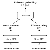
Figure 3. High-level architecture of linns

4.1. Machine Learning Basics

We begin by defining the machine learning problem we aim to solve and set the notation for the rest of this section.

Machine Learning Problem

Recall that our training data $D$ is a set $\{\langle{(\iota_{i}^{\#},f_{i}^{\#}),y_{i}}\rangle\}_{i},$ where $y_{i}$ is the label for intent $\iota^{\#}_{i}$ and filter $f^{\#}_{i}$. Let $H$ be a hypothesis space—a set of possible classifiers. A loss function $\ell:H\times Z\rightarrow\mathbb{R}$ defines how far the prediction of $H$ is on some item $z\in(I^{\#}\times F^{\#})\times Y$. Our goal is to minimize the loss function over the training set; we thus define the following quantity: $L_{D}(h)=\frac{1}{n}\sum_{j=1}^{n}\ell(h,\langle{(\iota_{j}^{\#},f_{j}^{\#}),y_{j}}\rangle)$.

Finally, we solve $\operatorname*{argmin}_{h\in H}\ L_{D}(h),$ which results in a hypothesis $h\in H$ that minimizes $L_{D}(h)$. This is typically performed using an optimization algorithm like stochastic gradient descent (sgd).

Notation

In what follows, we use $x,y,z,w,\ldots$ to denote column vectors in $\mathbb{R}^{n}$. We will use $\boldsymbol{x},\boldsymbol{y},\boldsymbol{z},\boldsymbol{w},\ldots$ to denote matrices in $\mathbb{R}^{n\times m}$, where $\boldsymbol{x}_{i}$ will denote the $i^{\emph{th}}$ column vector in matrix $\boldsymbol{x}$.

Neural Networks

Neural networks are transformations described in the form of matrix operations and pointwise operations. In general, a neural network $y=g(x;w)$ maps input $x$ to output $y$ with some vector $w$ called the parameters of the neural network, which are to be optimized to minimize the loss function. There are also other parameterizable aspects of a neural network, such as the dimensions of input and output, which need to be determined before training. Those are called hyperparameters.

4.2. Overview of Neural Architectures

We now briefly describe a number of neural network architectures we can use in tdes.

Multilayer Perceptrons (mlp)

Multilayer perceptrons are the canonical deep neural networks. They are compositions of multiple fully connected layers, which are functions of the form $\mathit{fc}({x};\boldsymbol{w},{b})=a(\boldsymbol{w}^{\top}{x}+{b}):\mathbb{R}^{m}\to\mathbb{R}^{n}$, where $\boldsymbol{w}$ and $b$ are parameters, $m$ is the input dimension, $n$ is the output dimension, and $a$ is a pointwise activation function. Some common activation functions include sigmoid and rectified linear unit (ReLU), respectively: ${\sigma}(x)=\frac{1}{1+e^{-x}}$ and $\operatorname{relu}(x)=max(0,x)$.

Convolutional Neural Networks (cnn)

cnns were originally developed for image recognition, and have recently been successfully applied to natural language processing (Kim, 2014; Kim et al., 2016). cnns are fast to train (compared to rnns; see below) and good at capturing shift invariant features, inspiring our usage here for encoding strings. In our setting, we use 1-dimensional cnns with global pooling, transforming a sequence of vectors into a single vector, i.e., $\mathbb{R}^{n\times l}\to\mathbb{R}^{k}$, where $l$ is the length of the input and $k$ is the number of kernels. Kernels are functions $\mathbb{R}^{n\times s}\to\mathbb{R}$ of size $s$ that are applied to every contiguous sequence of length $s$ of the input. A global pooling function (e.g., $\max$) then summarizes the outputs of each kernel into a single number. We use cnns by Kim et al. (2016) for encoding natural language, where kernels have variable size.

Recurrent Neural Networks (rnn)

rnns are effective at handling sequential data (e.g., text) by recursively applying a neural network unit to each element in the sequence. An rnn unit is a network mapping an input and hidden state pair at position $i-1$ in the sequence to the hidden state at position $i$, that is, $\emph{rnn\_unit}:\boldsymbol{x}_{i},h_{i-1}\mapsto h_{i}.$ The hidden state $h_{i}\in\mathbb{R}^{n}$ can be viewed as a summary of the sequence seen so far. Given a sequence $\boldsymbol{x}\in\mathbb{R}^{m\times l}$ of length $l$, we can calculate the final hidden state by applying the rnn unit at each step. Thus, we view an rnn as a transformation in $\mathbb{R}^{m\times l}\to\mathbb{R}^{n}$.

Practically, we use a long short-term memory network (lstm) (Hochreiter and Schmidhuber, 1997), an rnn designed to handle long-term dependencies in a sequence.

Recursive Neural Networks

Analogous to rnns, recursive neural networks apply the same unit over recursive structures like trees. A recursive unit takes input $x_{v}$ associated with tree node $v$ as well as all the hidden states $\boldsymbol{h}_{C(v)}\in\mathbb{R}^{n\times|C(v)|}$ from its children $C(v)$, and computes the hidden state $h_{v}$ of the current node. Intuitively, the vector $h_{v}$ summarizes the subtree rooted at $v$.

One popular recursive architecture is Tree-lstm (Tai et al., 2015). Adapted from lstms, a Tree-lstm unit can take possibly multiple states from the children of a node in the tree. For trees with a fixed number $k$ of children per node and/or the order of children matters, we can have dedicated weights for each child. This is called a $k$-ary Tree-lstm unit, a function in $\mathbb{R}^{n\times k}\to\mathbb{R}^{n}$. For trees with variable number of children per node and/or the order of children does not matter, we can operate over the sum of children states. This is called a Child-Sum Tree-lstm unit, a function in $\mathbb{R}^{n\times|C(v)|}\to\mathbb{R}^{n}$ for node $v$. Refer to Tai et al. (2015, Section 3) for details.

4.3. Type-Directed Encoders

We are ready to describe how we construct type-directed encoders (tde). A tde takes an abstract intent or filter and turns it into a real-valued vector of size $n$. As we shall see, however, our construction is generic: we can take some type $\tau$ and construct a tde for $\tau$ by recursively constructing encoders for constituents of $\tau$. Consider, e.g., a product type comprised of an integer and a string. An encoder for such type takes a pair of an integer and a string and returns a vector in $\mathbb{R}^{n}$. To construct such an encoder, we compose two separate encoders, one for integers and one for strings.

Formal Definition

Formally, an encoder for elements of type $\tau$ is a function $g:\tau\to\mathbb{R}^{n}$ mapping values of type $\tau$ into vector space $\mathbb{R}^{n}$. For element $a\in\tau$, $g(a)$ is called the encoding of $a$ by $g$. Integer $n$ is the dimension of the encoding, denoted by $\dim(g)=n$.

The dimension $n$ of an encoder is a fixed parameter that we have to choose—a hyperparameter. The intuition is that the larger $n$ is, the encoder can potentially capture more information, but will require more data to train.

Encoder Construction Framework

In what follows, we begin by describing encoders for base types: reals and characters. Then, we describe encoders for lists, sets, product types, and sum types. In our setting of icc analysis, these types appear in, for example, the intent action field, which is a list of characters (string) or null, and filter actions, which are sets of lists of characters (sets of strings).

The inference rules in Figure 4 describe how an encoder $g$ can be constructed for some type $\tau$, denoted by $g\blacktriangleright\tau$. Table 1 lists the parameters used by a tde, which are differentiable functions; the table also lists possible instantiations. Depending on how we instantiate these functions, we arrive at different encodersNote that tdes are compositions of differentiable functions; this is important since we can jointly train them along with the classifier in linns.

Example 4.1.

Throughout our exposition, we shall use the running example of encoding an abstract intent $\iota^{\#}$. We will use $\mathrm{L}(\tau)$ to denote the type of lists of elements in type $\tau$, and $\mathrm{S}(\tau)$ to denote sets of elements in $\tau$. We use $\Omega$ to denote the singleton type that only contains the undefined value $\omega$.

With this formalism, the type of an abstract intent is $(\mathrm{L}(\Sigma)+\Omega)\times\mathrm{S}(\mathrm{L}(\Sigma))$. $(\mathrm{L}(\Sigma)+\Omega)$ is a sum type, denoting that an action is either a string (list of characters) or null. Type $\mathrm{S}(\mathrm{L}(\Sigma))$ is that of categories of an abstract intent—sets of strings. The product $(\times)$ of action and categories comprises an abstract intent. Following Figure 4, the construction proceeds in a bottom-up fashion, starting with encoders for base types and proceeding upwards. For instance, to construct an encoder for $\mathrm{L}(\Sigma)$, we first require an encoder $g$ for type $\Sigma$, as defined by the rule e-list.

tensy  e-real $\displaystyle\lambda x\ldotp x\blacktriangleright\mathbb{R}$           tensy $\displaystyle\penalty 1\mathit{enumEnc}:\tau_{c}\rightarrow\mathbb{R}^{n}$  e-cat $\displaystyle\mathit{enumEnc}\blacktriangleright\tau_{c}$

tensy $\displaystyle\penalty 1\begin{array}[]{c}g:\tau\rightarrow\mathbb{R}^{n}\vspace{1pt}\\ \mathit{flat}:\mathrm{L}(\mathbb{R}^{n})\rightarrow\mathbb{R}^{m}\vspace{2pt}\end{array}$  e-list $\displaystyle\lambda x\ldotp\mathit{flat}(\emph{map}\ g\ x)\blacktriangleright\mathrm{L}(\tau)$       tensy $\displaystyle\penalty 1\begin{array}[]{c}g:\tau\rightarrow\mathbb{R}^{n}\vspace{1pt}\\ \mathit{aggr}:\mathrm{S}(\mathbb{R}^{n})\rightarrow\mathbb{R}^{m}\vspace{2pt}\end{array}$  e-set $\displaystyle\lambda x\ldotp\mathit{aggr}(\emph{map}\ g\ x)\blacktriangleright\mathrm{S}(\tau)$

tensy $\displaystyle\penalty 1g_{1}:\tau_{1}\rightarrow\mathbb{R}^{n}\quad g_{2}:\tau_{2}\rightarrow\mathbb{R}^{m}\quad\mathit{comb}:\mathbb{R}^{n}\times\mathbb{R}^{m}\rightarrow\mathbb{R}^{l}$  e-prod $\displaystyle\lambda(x,y)\ldotp\mathit{comb}(g_{1}(x),g_{2}(y))\blacktriangleright\tau_{1}\times\tau_{2}$

tensy $\displaystyle\penalty 1g_{1}:\tau_{1}\rightarrow\mathbb{R}^{n}\quad g_{2}:\tau_{2}\rightarrow\mathbb{R}^{n}$  e-sum $\displaystyle\lambda x\ldotp\emph{if}\ \ x\in\tau_{1}\ \emph{then}\ \ g_{1}(x)\ \ \emph{else}\ \ g_{2}(x)\blacktriangleright\tau_{1}+\tau_{2}$

$\tau_{c}$ is a categorical type, e.g., characters.

Figure 4. Rules for type-directed encoding. Representations of functions $\mathit{enumEnc}$, $\mathit{flat}$, $\mathit{aggr}$, $\mathit{comb}$, are in Table 1.

Table 1. Types of differentiable functions used in tdes (Figure 4) and possible practical instantiations

Encoder	Type	Possible differentiable implementations
$\mathit{enumEnc}$	$\Sigma\rightarrow\mathbb{R}^{l}$	Trainable lookup table (embedding layer)
$\mathit{flat}$	$\mathrm{L}(\mathbb{R}^{n})\rightarrow\mathbb{R}^{m}$	cnn / lstm
$\mathit{aggr}$	$\mathrm{S}(\mathbb{R}^{n})\rightarrow\mathbb{R}^{m}$	sum / Child-sum Tree-lstm unit
$\mathit{comb}$	$\mathbb{R}^{n}\times\mathbb{R}^{m}\rightarrow\mathbb{R}^{l}$	Single-layer mlp / binary Tree-lstm unit

Encoding Base Types

We start with encoders for base types.

Numbers

Since real numbers are already unary vectors, we can simply use the identity function ($\lambda x\ldotp x$) to encode elements of $\mathbb{R}$. This is formalized in the rule e-real. (The same applies to integers.)

Categorical types (chars)

We now consider types $\tau_{c}$ with finitely many values, e.g., ascii characters, Booleans and user-defined enumerated types. One common encoding is using a lookup table. Suppose there are $k$ possible values of type $\tau_{c}$, namely, $a_{1},a_{2},\dots,a_{k}$. The lookup table is often denoted as a matrix $\boldsymbol{w}\in\mathbb{R}^{n\times k}$, where $n$ is the dimension of the resulting encoding. The encoding for value $a_{j}$ is simply the $j^{\emph{th}}$ column $\boldsymbol{w}^{j}$ of the matrix $\boldsymbol{w}$.

As formalized in rule e-cat in Figure 4, we encode categorical types using an $\mathit{enumEnc}$ function, which we implement as a lookup table whose elements $\boldsymbol{w}$ are learned automatically.

Example 4.2.

In our example, we need two instances of $\mathit{enumEnc}$: $\mathit{enumEnc}_{\Sigma}$ for encoding characters in $\Sigma$, and $\mathit{enumEnc}_{\Omega}$ for encoding the null type $\Omega$.

Encoding Compound Types

We now switch attention to encoding compound types.

Lists

As formalized in rule e-list, to generate an encoder for $\mathrm{L}(\tau)$, we require an encoder for type $\tau$. Given an encoder $g:\tau\rightarrow\mathbb{R}^{n}$, we can apply it to every element of the list, thus resulting in a list of type $\mathrm{L}(\mathbb{R}^{n})$. Then, using the function $\mathit{flat}:\mathrm{L}(\mathbb{R}^{n})\rightarrow\mathbb{R}^{m}$, we can transform $\mathrm{L}(\mathbb{R}^{n})$ to a vector $\mathbb{R}^{m}$. As we indicate in Table 1, we use a cnn or an lstm to learn the function $\mathit{flat}$ during training.

Example 4.3.

To encode strings $\mathrm{L}(\Sigma)$ (actions), we construct

$$\emph{strEnc}=\lambda x\ldotp\mathit{flat}(\emph{map}\ \mathit{enumEnc}_{\Sigma}\ x)\blacktriangleright\mathrm{L}(\Sigma)$$

where $\mathit{enumEnc}_{\Sigma}$ is the encoder we construct for characters, and map is the standard list combinator that applies $\mathit{enumEnc}_{\Sigma}$ to every element in list $x$, resulting in a new list.

Sets

Rule e-set generates an encoder for type $\mathrm{S}(\tau)$, in an analogous manner to e-list. Given an encoder $g:\tau\rightarrow\mathbb{R}^{n}$, we can apply it to every element of the set, thus resulting in a set of type $\mathrm{S}(\mathbb{R}^{n})$. Then, using the aggregation function $\mathit{aggr}:\mathrm{S}(\mathbb{R}^{n})\rightarrow\mathbb{R}^{m}$, we can transform $\mathrm{S}(\mathbb{R}^{n})$ to a vector $\mathbb{R}^{m}$. As shown in Table 1, we can simply set $\mathit{aggr}$ to be the sum of all vectors in the set, or use a Child-sum Tree-lstm unit to pool all elements of a set.

Note that our treatment of sets differs from lists: We do not use cnns or lstms to encode sets, since, unlike lists, sets have no ordering on elements to be exploited by a cnn or an lstm.

Example 4.4.

Categories of an intent are of type $\mathrm{S}(\mathrm{L}(\Sigma))$. Given an encoder strEnc for $\mathrm{L}(\Sigma)$, we construct the encoder

$$\emph{catsEnc}=\lambda x\ldotp\emph{aggr}(\emph{map}\ \emph{strEnc}\ x)\blacktriangleright\mathrm{S}(\mathrm{L}(\Sigma))$$

where map here applies strEnc to every element in set $x$.

Sum Types

We now consider sum (union) types $\tau_{1}+\tau_{2}$, where a variable can take values in $\tau_{1}$ or $\tau_{2}$. Rule e-sum generates an encoder for type $\tau_{1}+\tau_{2}$; it assumes that we have two encoders, $g_{1}$ and $g_{2}$, for $\tau_{1}$ and $\tau_{2}$, respectively. Both encoders have to map vectors of the same size $n$. e-sum generates an encoder from $\tau_{1}+\tau_{2}$ to a vector in $\mathbb{R}^{n}$. If a variable $x$ is of type $\tau_{1}$, it is encoded as the vector $g_{1}(x)$. Alternatively, if $x$ is of type $\tau_{2}$, it is encoded as the vector $g_{2}(x)$.

Example 4.5.

The action field of an abstract intent is a sum type $\mathrm{L}(\Sigma)+\Omega$; We construct an encoder for this as follows:

$$\emph{actEnc}=\lambda x\ldotp\emph{if}\ x\in\mathrm{L}(\Sigma)\ \emph{then}\ \emph{strEnc}(x)\ \emph{else}\ \mathit{enumEnc}_{\Omega}(x)\blacktriangleright\mathrm{L}(\Sigma)+\Omega$$

Product Types

We now consider product types of the form $\tau_{1}\times\tau_{2}$. Rule e-prod generates an encoder for type $\tau_{1}\times\tau_{2}$; as with e-sum, it assumes that we have two encoders, $g_{1}$ and $g_{2}$, one for type $\tau_{1}$ and another for $\tau_{2}$. Additionally, we assume we have a function $\mathit{comb}:\mathbb{R}^{n}\times\mathbb{R}^{m}\rightarrow\mathbb{R}^{l}$. The encoder for $\tau_{1}\times\tau_{2}$ therefore encodes type $\tau_{1}$ using $g_{1}$, encodes type $\tau_{2}$ using $g_{2}$, and then summarizes the two vectors produced by $g_{1}$ and $g_{2}$ as a single vector in $\mathbb{R}^{l}$. This can be performed using an mlp, or using a binary Tree-lstm unit. Essentially, we view the the product type as a tree node with 2 children; so we can summarize the children using a Tree-lstm unit.

Example 4.6.

Finally, to encode an intent, we encode the product type of an action and categories:

$$\lambda(a,c)\ldotp\mathit{comb}(\emph{actEnc}(a),\emph{catsEnc}(b))\blacktriangleright(\mathrm{L}(\Sigma)+\Omega)\times\mathrm{S}(\mathrm{L}(\Sigma))$$

Table 2. Instantiations of tde parameters

		tde parameters
Instantiation	Type	$\mathit{enumEnc}$	$\mathit{flat}$	$\mathit{aggr}$	$\mathit{comb}$
str-rnn	$\mathrm{L}(\Sigma)$	lookup	rnn	-	-
str-cnn	$\mathrm{L}(\Sigma)$	lookup	cnn	-	-
typed-simple	full	lookup	cnn	sum	1-layer perceptron
typed-tree	full	lookup	cnn	Tree-lstm	Tree-lstm

*lookup stands for lookup table, as described in §4.3 and Table 1.

Table 3. Choices of hyperparameters

Hyperparameter		Choice
Lookup table	dimension	16
cnn	kernel sizes	$\langle 1,3,5,7\rangle$
	kernel counts	$\langle 8,16,32,64\rangle$
	activation	$\operatorname{relu}$
	pooling	max
rnn (lstm)	hidden size	128
1-layer perceptron	dimensions	64
	activation	$\operatorname{relu}$
Multilayer perceptron	dimensions	$\langle 16,1\rangle$
	activation	$\langle\operatorname{relu},\sigma\rangle$

5. Implementation and Evaluation

We now describe an implementation of our technique with various instantiations and present a thorough evaluation. We designed our evaluation to answer the following two questions:

Q1: Accuracy:

Are linns effective at predicting may links, and what are the best instantiations of tdes for our task?

Q2: Efficiency:

What is the runtime performance of model training and link prediction (inference)?

We begin by summarizing our findings:

1. The best instantiation of tdes labels may links with an F1 score of 0.931, an area under roc curve of 0.991, and a Kruskal’s $\gamma$ of 0.992. All these metrics indicate high accuracy.

2. All instantiations complete training within $\sim$20min. All instantiations take $<$0.2ms to label a link, except the instantiation using rnns, which takes 2.2ms per link.

Instantiations

To answer our research questions, we experiment with 4 different instantiations of tdes, outlined in Table 2, which are designed to vary in model sophistication, from simplest to most complex. In the simplest instantiations, str-rnn and str-cnn, we serialize abstract intents and filters as strings ($\mathrm{L}(\Sigma)$) and use rnns and cnns for encoding. In the more complex instantiations, typed-simple and typed-tree, we maintain the full constituent types for intents and filters, as illustrated in §4.3. The typed-simple instantiatition uses the simplest choices for $\mathit{aggr}$ and $\mathit{comb}$—sum of all elements and a single-layer neural network, respectively. The typed-tree instantiations uses Child-Sum and binary Tree-lstm units instead.

Hyperparameters

Table 3 summarizes the choice of hyperparameters. We choose the embedding dimension and the range of kernel sizes following a similar choice as in Kim et al. (2016). We choose only odd sizes for alignment consideration. We choose $\operatorname{relu}$ for all activations as it is both effective in prediction and efficient in training. For global pooling in cnns, $\max$ is used as we are only interested in the existence of a pattern, rather than its frequencies. The hidden size of rnns is set close to the output size of cnns, so we could fairly compare the capability of the two architectures. Tree-lstms used in our instantiations require no hyperparameterization, as the hidden size is fixed to the output size of the string encoder.

Implementation

We have implemented our instantiations in Python using Keras (Chollet, 2015) with the TensorFlow (Abadi et al., 2016) backend. We chose cross entropy as our loss function and RMSprop (Tieleman and Hinton, 2012), a variation of stochastic gradient descent (sgd), for optimization. All experiments were performed on a machine with an Intel Core i7-6700 (3.4 GHz) CPU, 32GB memory, 1TB SSD, and Nvidia GeForce GTX 970 GPU. The linn was trained and tested on the GPU.

5.1. Experimental Setup

Corpus

We used the primo (Octeau et al., 2016a) corpus, consisting of 10,500 Android applications from Google Play. For static analysis, we used ic3 (Octeau et al., 2015) combined with primo’s abstract matching procedure. This combination provides a definitive must/may label to pairs of abstract intents and filters.

Simulating Imprecision

The challenge with setting up the training and test data is that we do not know the ground truth label of may links. To work around that, we adopt the ingenious approach of Octeau et al. (2016a), who construct synthetic may links from must links by instilling imprecisions in abstract intents and filters. This results in a set of may links for which we know the label. Formally, to add imprecision to an abstract intent $\iota^{\#}$, we transform it into a weaker abstract value $\iota_{w}^{\#}$ such that $\iota^{\#}\subseteq\iota_{w}^{\#}$. Intuitively, adding imprecisions involves adding regular expressions, like ".*" into, e.g., action strings.

Following (Octeau et al., 2016a), we use the empirical distribution of imprecision observed in the original abstract intents (filters) to guide the imprecision simulation process. Specifically, we distinguish the different types of imprecision (full or partial, and by each field) and calculate the empirical probability for each of them as they appear in our data. These probabilities are then used to introduce respective imprecisions in the intents and filters. Note that the introduction of imprecision does not necessarily convert a must link into a may link—since even if we weaken an abstract intent, the abstract matching process may still detect its label definitively.

Sampling and Balancing

We train the model on a sampled subset of links, as the number of links is quadratic in the number of intents and filters and training is costly (we have 3,856 intents and 37,217 filters, leading to over 100 million links). Sampling may result in loss of information; however, as we show, our models perform well.

Another important aspect of sampling is balancing. Neural networks are sensitive to a balanced presence of positive and negative training instances. In our setting, links over some particular intent (filter) could easily fall into one of two extreme cases where most of them are positive (intent is vague) or most of them are negative (intent is specific). So we carefully sample links balanced between positive and negative labels, and among intents (filters). Sampling and balancing led to a training set consisting of 105,108 links, (63,168 negative and 41,940 positive), and a testing set consisting of 43,680 links (29,260 negative and 14,420 positive). Note that the testing set is comprised solely of may links.

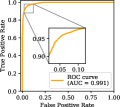
(a) Receiver operating characteristic (roc)

(b) Distribution of predicted link probabilities

Figure 5. Detailed results for the typed-tree instantiation

Table 4. Summary of model evaluations

Instantiation	# Parameters	Inference time ($\mu$s/link)	Testing $\gamma$	Testing F1	auc	Entropy of $\hat{y}$	$\emph{Pr}(y=1\mid\hat{y}>0.95)$	$\emph{Pr}(\hat{y}>0.95)$
str-rnn	154,657	2220	0.970	0.891	0.975	3.002	0.980	0.089
str-cnn	27,409	57	0.988	0.917	0.988	2.534	0.998	0.139
typed-simple	142,417	157	0.989	0.920	0.988	2.399	0.996	0.173
typed-tree	634,881	171	0.992	0.931	0.991	2.220	0.994	0.200

5.2. Results

Q1: Accuracy

To measure the predictive power of our four instantiations, we use a number standard metrics:

• F1 score is the harmonic mean of precision and recall, which gives a balanced measure of a predictor’s false-negative and false-positive rates. When computing F1, the model output is rounded to get a 0/1 label. A value of 1 indicates perfect precision/recall.

• Receiver operating characteristic (roc) curve plots the true-positive rate against the false-positive rate. It represents a binary classifier’s diagnostic performance at different discrimination thresholds. A perfect model has an area under the curve (auc) of 1.

• Kruskal’s $\gamma$ is used to measure the correlation between the ranking computed by our model and the ground truth on may links, which is useful in our setting as in practice we would use computed probabilities to rank may links in order of likelihood to present them to the user for investigation. A value of 1 indicates perfect correlation between computed ranking and ground truth.

The metrics for each instantiation are summarized in Table 4. In addition to the aforementioned metrics, we include the number of trainable parameters, indicating the fitting power (lower is better); inference time (time to evaluate one instance); entropy of predicted probabilities $\hat{y}$, indicating the power of triaging links (lower is better); probability of true positives within links with high predicted values $\emph{Pr}(y=1\mid\hat{y}>0.95)$ (higher is better); and portion of links with such high predicted values $\emph{Pr}(\hat{y}>0.95)$ (higher is better).

We observe that the best instantiation is typed-tree. Note, however, that using Tree-lstm involves the largest number of trainable parameters. With the fewest trainable parameters and fastest running time, the str-cnn model achieves the highest true-positive rate within the most highly ranked links. The str-rnn model is worse than others in almost all aspects, suggesting that the rnn string encoder struggles to capture useful patterns from intents (filters). Our results show that more complex models, specifically those that use more parameters or encode more structure, tend to perform slightly better. While simple models are good enough, more complex models may still lend significant advantage when we consider market-scale analysis: link inference has to run on millions of links and even small differences (e.g. a false positive rate difference of just 0.49% between our two best models, typed-tree and typed-simple) would translate to thousands of mislabeled links.

Figure 5(a) shows the roc curve over the testing dataset for the typed-tree model. Figure 5(b) shows the distribution of the predicted probabilities of the existence of a link, and the probability of a link actually existing given the predicted probability. The curve depicting the conditional probability would ideally follow $y=x$ line. Therefore, the model’s prediction value is highly correlated to the true probability of being a positive, which confirms with the high $\gamma$ value we observed. A higher value at the upper right of the conditional probability curve suggests links highly ranked ($\hat{y}$ ¿ 0.95) by our models are highly likely actual positives. This is particularly important in saving the effort of humans involved in investigating links.

Compared to primo (Octeau et al., 2016a), our evaluation is over a set of may links only. This is a strictly more difficult setting than primo’s, which evaluated over all links containing any imprecision—so some of the links are actually must links. In particular, if a link is must not exist, a partially imprecise version will also mostly be must not exist. For example, a(.*)c does not match xyz. Despite working in a more challenging setting, our best instantiations are still able to achieve a Kruskal’s $\gamma$ value $(0.988-0.992)$ higher than primo $(0.971)$ (In fact, if we use the same setting as primo, our Kruskal’s $\gamma$ reaches $0.999$.)

Q2: Efficiency

Regarding running time, all our instantiations, except str-rnn, are efficient. As shown in Table 4, they take no more than 171µs per link for inference. The training time is proportional to inference time. The three best instantiations take no more than 20min to finish 10 epochs of training. We consider this particularly fast, given that we used only average hardware and deep-neural-network training often lasts several hours or days for many problems. The only exception is str-rnn, which is about 13 times slower than the slowest of the other three, mainly because of the inefficient unrolling of rnn units over long input strings.

The storage costs or the model size can be measured in the number of trainable parameters. As shown in Table 4, the largest model (typed-tree) consists of about 634K parameters, taking up 5.6 MB on disk; the smallest model (string-cnn) consists of only about 27K parameters, taking up merely 300KB on disk. In summary, even the most complex model does not have significant storage cost.

Threats to Validity

We see two threats to validity of our evaluation. First, to generate labeled may links for testing, we synthetically instilled imprecision, following the methodology espoused by primo, enabling a head-to-head comparison with primo. While the synthetic imprecision follows the empirical imprecision distribution, we could imagine that actual may links only exhibit rare, pathological imprecisions. While we cannot discount this possibility, we believe it is unlikely. The ultimate test of our approach is in improving the efficacy of client analyses such as IccTA (Li et al., 2015) and we intend to investigate the impact of client analyses in future work.

Second, with neural networks, it is often unclear whether they are capturing relevant features or simply getting lucky. To address this threat, we next perform an interpretability investigation.

6. Interpretability Investigation

We now investigate whether our models are learning the right things and not basing predictions on extraneous artifacts in the data. An informal way to frame this concern is whether the model’s predictions align with human intuition. This is directly associated with the trust we can place on the model and its predictions (Ribeiro et al., 2016).

Our efforts towards interpretability are multifold:

• We analyzed the incorrect classifications to understand the reasons for incorrectness. Our analysis indicates that the reasons for incorrectness are understandable and intuitively explained. (§6.1)

• We analyze several instances to understand what parts of input are important for the predictions. Results show that the model is taking expected parts of the inputs into account. (§6.2)

• We studied activations of various kernels inside the neural networks to see which inputs activated them the most. Our findings show several recognizable strings, which intuitively should have a high influence on classification, to be activating the kernels. (§6.3)

• We used t-SNE visualizations (Maaten and Hinton, 2008) to understand how a model groups similar inputs and what features it may be using. We found several important patterns, boosting our trust in the model. (§6.4)

Interpreting and explaining predictions of a ML-algorithm is a challenging problem and in fact a topic of active research (Gunning, [n. d.]; Wierzynski, 2018). Our study in this section is thus a best-effort analysis.

6.1. Error Inspection

We present anecdotal insights from our investigation of erroneous classification in the typed-simple model. A number of misclassifications appear where the action or category fields are completely imprecise (e.g., action string is (.*)) or too imprecise to make meaningful deductions. The model unsurprisingly has difficulty in classifying such cases.

There are also, albeit fewer, misclassified instances for near-certain matches. Examples include android.intent.action.VIEW matching against android.intent.action(.*)EW and android.intent.action.GET_C(.*)NTENT matching against android.intent. action.GET_CONTENT (as part of intents and filters). Such misses may be due to imprecision preventing encoders from detecting characteristic patterns (e.g. (.*)EW is seemingly very different from VIEW). Finally, Our model predicts a matches for different but very similar strings. For example, consider com.andromo. dev48329.app53751.intent.action.FEED_STAR(.*)ING and com. andromo.d(.*)9.app135352.intent.action.FEED_STARTING. The two look similar but have different digits We explore this case more in § 6.4.

Overall, our model is able to extract and generalize useful patterns. However, it probably has less grasp on the exact meaning of (.*), so there are failures to identify some highly probable matches.

Figure 6. Explaining individual instances

6.2. Explaining Individual Instances

We would like to explain predictions on individual instances. Our approach is similar to that of the popular system lime (Ribeiro et al., 2016): we perturb the given instance and study change in prediction of the model, treated as a black box, due to the perturbation. In this way, we can “explain” the prediction on the given instance. We used the str-cnn instantiation and perturbed the string representation of the given intent while keeping the filter string constant. Our perturbation technique is to mask (delete) a substring from the string. We perform this perturbation at all locations of the string. Using a mask length of 5, the examples in Figure 6 show intents and filters with a heat map overlaid on the intents while keeping the filters uncolored. All the instances selected here have positive link predictions (it is unlikely to perturb a negatively predicted link to result in a positive prediction). The redder regions indicate a significant difference in prediction when masking around those regions, thus indicating that the regions are important for the predictions.

The examples generally show red regions in the action and categories values, which implies that those values are important for the prediction. Thus, the model is generally making good decisions about what is important. There are a couple of outliers. First, the second instance does not have the action field reddened. This is probably because there is no direct match between the action strings in the intent and filter and it may just be the case that the model was learnt from similar examples in the training set. The other outlier is the third-last example: we believe that masking any small part of the action still leaves enough useful information, which the model can pick up to make a positive prediction. Overall, these examples give us confidence that the model has acquired a reasonably correct understanding of intent resolution.

6.3. Studying Kernel Activations

We tested input strings on the str-cnn instantiation to find if the cnn kernels are picking up patterns relevant to icc link inference. We went over all intent strings in our dataset and for each cnn kernel, looked for string segments that activate the kernel the most. Some representative kernels and their top activating segments are shown in Table 5. Important segments are noticeable. For example, kernel conv1d_size5:14 gets activated on (.*), and kernel conv1d_size7:0 gets activated on VIEW. Kernel conv1d_size5:3 is interesting, as it seems to capture null, an important special value, but also captures sulle. This indicates a single kernel on its own may not be so careful at distinguishing useful vs. less useful but similar looking segments. Apart from such easily interpretable cases, many other activations appear for seemingly meaningless strings. It is likely that in combination, they help capture subtle context, and when combined in later layers, generate useful encodings.

Table 5. Some cnn kernels and their top stimuli

conv1d_size5:14		conv1d_size5:3		conv1d_size7:0
segment	activation	segment	activation	segment	activation
(.*)R	1.951	null}	3.796	TAVIEWA	3.704
(.*)u	1.894	null,	2.822	n.VIEW"	3.543
(.*)t	1.893	sulle	2.488	y.VIEW"	3.384

6.4. Visualization of Encodings

We present a visualization to discover interesting patterns in encodings. In the interest of space, we only discuss intent encodings for the typed-simple instantiation. We use t-SNE (Maaten and Hinton, 2008), a non-linear dimensionality reduction technique frequently used for visualizing high-dimensional data in two or three dimensions. The key aspect of the technique is that similar objects are mapped to nearby points while dissimilar objects are mapped to distant points. Figure 8 shows the encodings for all intents in the training set (sub-figures highlight different areas). The size of each point reflects the number of intents sharing the same combination of values.

(a) android.intent.*

(b) Imprecise VIEW actions

(c) dev*.app*.*.FEED*

(d) DEFAULT, total imprecise and null categories

Figure 8. Intent encodings visualized using t-SNE

Figure 8(a) highlights the intents for which the action starts with android.intent. The top cluster is associated with category android.intent.category.DEFAULT and the bottom is associated with null categories. A few different actions comprise the top cluster, e.g., android.intent.action.VIEW, android.intent.action.SEND, and imprecise versions of these actions. Figure 8(b) zooms in on the top cluster to show six imprecise versions of the VIEW action: one top circle containing android.inte(.*).VIEW; three circles containing android.intent(.*)n.VIEW, android.intent.(.*)n.VIEW, and android.intent(.*).VIEW; and two lower-figure circles containing an(.*)ction.VIEW and a(.*)action.VIEW. We can thus see the level of imprecision reflected spatially, while the semantic commonality is still well preserved as the points are all close to the big circle of the precise value.

Figure 8(c) highlights actions whose last part starts with FEED. The prefixes are largely different but share the pattern of dev*.app*, where * are strings of digits. Our model is thus able to extract the common pattern and generate similar encodings for these intents.

The last example is the effect of three important values of the categories field: {android.intent.category.DEFAULT}, total imprecision {(.*)}, and { }. In Figure 8(d), we highlight three encodings with the VIEW action and the above categories. The encoding for that of { } (bottom circle) is separated from the other two (top circle). This conforms with the fact that total imprecision is the imprecise version of some concrete value, which is most likely DEFAULT, rather than the absence of the value for the categories field, which means ignoring the field during resolution. Our observations suggest that our intent encoder is able to automatically learn semantic (as opposed to merely syntactic) artifacts.

7. Related Work

Android Analysis

The early ComDroid system (Chin et al., 2011) inferred subsets of icc values using simple, ad hoc static analysis. Epicc (Octeau et al., 2013) constructed a more detailed model of icc. ic3 (Octeau et al., 2016b) and Bosu et al. (2017) improved on Epicc by using better constant propagation. These static-analysis techniques inevitably overapproximate the set of possible icc values and can thus potentially benefit from our work. primo (Octeau et al., 2016a) was the first to formalize the icc link resolution process. We have compared with primo in Sections 1 and 5.

icc security studies range from information-flow analysis (Bosu et al., 2017; Gordon et al., 2015; Klieber et al., 2014; Li et al., 2015; Wei et al., 2014) to vulnerability detection (Bagheri et al., 2015; Li et al., 2014; Lu et al., 2012; Feng et al., 2014). These works do not perform a formal icc analysis and are instead consumers of icc analysis and can potentially benefit from our work.

Static Analysis Alarms

Z-Ranking (Kremenek and Engler, 2003) uses a simple counting technique to go through analysis alarms and rank them. Since bugs are rare, if the analysis results are mostly safe, but then an error is reported, then it is likely an error. Tripp et al. (2014) train a classifier using manually supplied labels and feature extraction of static analysis results. We utilize static analysis to automatically do the labeling, and perform feature extraction automatically from abstract values. Koc et al. (2017) use manually labeled data and neural networks to learn code patterns where static analysis loses precision. Our work uses automatically generated must labels, and since errors (links) are not localized in one line or even application, we cannot pinpoint specific code locations for training. Merlin (Livshits et al., 2009) infers probabilistic information-flow specifications from code and then applies them to discover bugs; similar approaches were also proposed by Kremenek et al. (2006) and Murali et al. (Murali et al., 2017). We instead augment static analysis with a post-processing step to assign probabilities to alarms.

Another class of methods uses logical techniques to suppress false alarms, e.g., using abduction (Dillig et al., 2012) or predicate abstraction (Blackshear and Lahiri, 2013).

ML for Programs

There is a plethora of works applying forms of machine learning to “big code”—see Allamanis et al. (2017a) for a comprehensive survey. We compare with most related works.

Related to tdes, Parisotto et al. (2017) introduced a tree-structured neural network to encode abstract-syntax trees for program synthesis. tdes can potentially be extended in that direction to reason about recursive data types. Allamanis et al. (2016) use cnns to generate summaries of code. Here, we used cnns to encode list data types.

Allamanis et al. (2017b) present neural networks that encode and check semantic equivalence of two symbolic formulas. The task is more strict than link inference. For our case, simple instantiations work reasonably well. It is also prohibitive to generate all possible intents or filters as they did for Boolean formulas.

Hellendoorn and Devanbu (Hellendoorn and Devanbu, 2017) proposed modeling techniques for source code understanding, which they test with n-grams and rnns. Gu et al. (Gu et al., 2016) use deep learning to generate api sequences for a natural language query (e.g., parse xml, or play audio). Instead of using deep learning for code understanding, we use it to classify imprecise results of static analysis for inter component communication. Raychev et al. (2014) use rnns for code completion and other techniques for predicting variable names and types (Raychev et al., 2015).

8. Conclusions

We tackled the problem of false positives in static analysis of Android communication links. We augment a static analysis with a post-processing step that estimates the probability with which a link is indeed a true positive. To facilitate machine learning in our setting, we propose a custom neural-network architecture targeting the link-inference problem. The key novelty is type-directed encoders (tde), a framework for composing neural networks that take elements of some type $\tau$ and encodes them into real-valued vectors. We believe that this technique can be applicable to a wide variety of problems in the context of machine-learning applied to programming-languages problems. In the future, we want to explore this intriguing idea in other contexts.

- (1)
- Abadi et al. (2016) Martín Abadi, Paul Barham, Jianmin Chen, Zhifeng Chen, Andy Davis, Jeffrey Dean, Matthieu Devin, Sanjay Ghemawat, Geoffrey Irving, Michael Isard, et al. 2016. TensorFlow: A System for Large-Scale Machine Learning.. In OSDI, Vol. 16. 265–283.
- Allamanis et al. (2017a) Miltiadis Allamanis, Earl T Barr, Premkumar Devanbu, and Charles Sutton. 2017a. A Survey of Machine Learning for Big Code and Naturalness. arXiv preprint arXiv:1709.06182 (2017).
- Allamanis et al. (2017b) Miltiadis Allamanis, Pankajan Chanthirasegaran, Pushmeet Kohli, and Charles Sutton. 2017b. Learning Continuous Semantic Representations of Symbolic Expressions. In International Conference on Machine Learning. 80–88.
- Allamanis et al. (2016) Miltiadis Allamanis, Hao Peng, and Charles Sutton. 2016. A Convolutional Attention Network for Extreme Summarization of Source Code. In Proceedings of The 33rd International Conference on Machine Learning (Proceedings of Machine Learning Research), Maria Florina Balcan and Kilian Q. Weinberger (Eds.), Vol. 48. PMLR, New York, New York, USA, 2091–2100. http://proceedings.mlr.press/v48/allamanis16.html
- Bagheri et al. (2015) H. Bagheri, A. Sadeghi, J. Garcia, and S. Malek. 2015. COVERT: Compositional Analysis of Android Inter-App Permission Leakage. IEEE Transactions on Software Engineering 41, 9 (Sept 2015), 866–886. https://doi.org/10.1109/TSE.2015.2419611
- Blackshear and Lahiri (2013) Sam Blackshear and Shuvendu K. Lahiri. 2013. Almost-correct Specifications: A Modular Semantic Framework for Assigning Confidence to Warnings. In Proceedings of the 34th ACM SIGPLAN Conference on Programming Language Design and Implementation (PLDI ’13). ACM, New York, NY, USA, 209–218. https://doi.org/10.1145/2491956.2462188
- Bosu et al. (2017) Amiangshu Bosu, Fang Liu, Danfeng (Daphne) Yao, and Gang Wang. 2017. Collusive Data Leak and More: Large-scale Threat Analysis of Inter-app Communications. In Proceedings of the 2017 ACM on Asia Conference on Computer and Communications Security (ASIA CCS ’17). ACM, New York, NY, USA, 71–85. https://doi.org/10.1145/3052973.3053004
- Chin et al. (2011) Erika Chin, Adrienne Porter Felt, Kate Greenwood, and David Wagner. 2011. Analyzing Inter-Application Communication in Android. In Proceedings of the 9th Annual International Conference on Mobile Systems, Applications, and Services (MobiSys).
- Chollet (2015) Francois Chollet. 2015. keras. https://github.com/fchollet/keras.
- Dillig et al. (2012) Isil Dillig, Thomas Dillig, and Alex Aiken. 2012. Automated Error Diagnosis Using Abductive Inference. In Proceedings of the 33rd ACM SIGPLAN Conference on Programming Language Design and Implementation (PLDI ’12). ACM, New York, NY, USA, 181–192. https://doi.org/10.1145/2254064.2254087
- Elish et al. (2015) Karim O Elish, Danfeng Yao, and Barbara G Ryder. 2015. On the need of precise inter-app ICC classification for detecting Android malware collusions. In Proceedings of IEEE mobile security technologies (MoST), in conjunction with the IEEE symposium on security and privacy.
- Enck et al. (2011) William Enck, Damien Octeau, Patrick McDaniel, and Swarat Chaudhuri. 2011. A Study of Android Application Security. In Proceedings of the 20th USENIX Security Symposium.
- Feng et al. (2014) Yu Feng, Saswat Anand, Isil Dillig, and Alex Aiken. 2014. Apposcopy: Semantics-Based Detection of Android Malware through Static Analysis. In Proceedings of the 22nd ACM SIGSOFT International Symposium on the Foundations of Software Engineering (FSE ’14).
- Goodfellow et al. (2016) Ian Goodfellow, Yoshua Bengio, and Aaron Courville. 2016. Deep learning. MIT press.
- Gordon et al. (2015) Michael I. Gordon, Deokhwan Kim, Jeff H. Perkins, Limei Gilham, Nguyen Nguyen, and Martin C. Rinard. 2015. Information Flow Analysis of Android Applications in DroidSafe. In 22nd Annual Network and Distributed System Security Symposium, NDSS 2015, San Diego, California, USA, February 8-11, 2015. http://www.internetsociety.org/doc/information-flow-analysis-android-applications-droidsafe
- Grace et al. (2012) Michael Grace, Yajin Zhou, Zhi Wang, and Xuxian Jiang. 2012. Systematic Detection of Capability Leaks in Stock Android Smartphones. In NDSS ’12.
- Gu et al. (2016) Xiaodong Gu, Hongyu Zhang, Dongmei Zhang, and Sunghun Kim. 2016. Deep API learning. In Proceedings of the 2016 24th ACM SIGSOFT International Symposium on Foundations of Software Engineering. ACM, 631–642.
- Gunning ([n. d.]) David Gunning. [n. d.]. Explainable Artificial Intelligence (XAI). Available from https://www.darpa.mil/program/explainable-artificial-intelligence.
- Hellendoorn and Devanbu (2017) Vincent J Hellendoorn and Premkumar Devanbu. 2017. Are deep neural networks the best choice for modeling source code?. In Proceedings of the 2017 11th Joint Meeting on Foundations of Software Engineering. ACM, 763–773.
- Hochreiter and Schmidhuber (1997) Sepp Hochreiter and Jürgen Schmidhuber. 1997. Long short-term memory. Neural computation 9, 8 (1997), 1735–1780.
- Kim (2014) Yoon Kim. 2014. Convolutional neural networks for sentence classification. In Proceedings of the 2014 Conference on Empirical Methods in Natural Language Processing (EMNLP ’14). Citeseer, 1746–1751.
- Kim et al. (2016) Yoon Kim, Yacine Jernite, David Sontag, and Alexander M Rush. 2016. Character-aware neural language models. In Proceedings of the Thirtieth AAAI Conference on Artificial Intelligence (AAAI ’16). AAAI Press, 2741–2749.
- Klieber et al. (2014) William Klieber, Lori Flynn, Amar Bhosale, Limin Jia, and Lujo Bauer. 2014. Android Taint Flow Analysis for App Sets. In Proceedings of the 3rd ACM SIGPLAN International Workshop on the State of the Art in Java Program Analysis (SOAP ’14). ACM, New York, NY, USA, 1–6. https://doi.org/10.1145/2614628.2614633
- Koc et al. (2017) Ugur Koc, Parsa Saadatpanah, Jeffrey S Foster, and Adam A Porter. 2017. Learning a classifier for false positive error reports emitted by static code analysis tools. In Proceedings of the 1st ACM SIGPLAN International Workshop on Machine Learning and Programming Languages. ACM, 35–42.
- Kremenek and Engler (2003) Ted Kremenek and Dawson Engler. 2003. Z-ranking: Using Statistical Analysis to Counter the Impact of Static Analysis Approximations. In Proceedings of the 10th International Symposium on Static Analysis (SAS’03). Springer-Verlag, Berlin, Heidelberg, 295–315. http://dl.acm.org/citation.cfm?id=1760267.1760289
- Kremenek et al. (2006) Ted Kremenek, Paul Twohey, Godmar Back, Andrew Ng, and Dawson Engler. 2006. From Uncertainty to Belief: Inferring the Specification Within. In Proceedings of the 7th Symposium on Operating Systems Design and Implementation (OSDI ’06). USENIX Association, Berkeley, CA, USA, 161–176. http://dl.acm.org/citation.cfm?id=1298455.1298471
- Li et al. (2015) Li Li, Alexandre Bartel, Tegawendé F. Bissyandé, Jacques Klein, Yves Le Traon, Steven Arzt, Siegfried Rasthofer, Eric Bodden, Damien Octeau, and Patrick McDaniel. 2015. IccTA: Detecting Inter-Component Privacy Leaks in Android Apps. In Proceedings of the 37th International Conference on Software Engineering (ICSE 2015).
- Li et al. (2014) Li Li, Alexandre Bartel, Jacques Klein, and Yves Le Traon. 2014. Automatically Exploiting Potential Component Leaks in Android Applications. In Proceedings of the 13th International Conference on Trust, Security and Privacy in Computing and Communications (TrustCom 2014). IEEE.
- Livshits et al. (2009) Benjamin Livshits, Aditya V. Nori, Sriram K. Rajamani, and Anindya Banerjee. 2009. Merlin: Specification Inference for Explicit Information Flow Problems. In Proceedings of the 30th ACM SIGPLAN Conference on Programming Language Design and Implementation (PLDI ’09). ACM, New York, NY, USA, 75–86. https://doi.org/10.1145/1542476.1542485
- Lu et al. (2012) Long Lu, Zhichun Li, Zhenyu Wu, Wenke Lee, and Guofei Jiang. 2012. CHEX: statically vetting Android apps for component hijacking vulnerabilities. In Proceedings of the 2012 ACM conference on Computer and communications security (CCS ’12). ACM, 229–240. https://doi.org/10.1145/2382196.2382223
- Maaten and Hinton (2008) Laurens van der Maaten and Geoffrey Hinton. 2008. Visualizing data using t-SNE. Journal of Machine Learning Research 9, Nov (2008), 2579–2605.
- Murali et al. (2017) Vijayaraghavan Murali, Swarat Chaudhuri, and Chris Jermaine. 2017. Bayesian specification learning for finding API usage errors. In Proceedings of the 2017 11th Joint Meeting on Foundations of Software Engineering. ACM, 151–162.
- Octeau et al. (2016a) Damien Octeau, Somesh Jha, Matthew Dering, Patrick McDaniel, Alexandre Bartel, Li Li, Jacques Klein, and Yves Le Traon. 2016a. Combining static analysis with probabilistic models to enable market-scale android inter-component analysis. In POPL, Vol. 51. ACM, 469–484.
- Octeau et al. (2015) Damien Octeau, Daniel Luchaup, Matthew Dering, Somesh Jha, and Patrick McDaniel. 2015. Composite Constant Propagation: Application to Android Inter-Component Communication Analysis. In Proceedings of the 37th International Conference on Software Engineering (ICSE). http://siis.cse.psu.edu/pubs/octeau-icse15.pdf
- Octeau et al. (2016b) D. Octeau, D. Luchaup, S. Jha, and P. McDaniel. 2016b. Composite Constant Propagation and its Application to Android Program Analysis. IEEE Transactions on Software Engineering 42, 11 (Nov 2016), 999–1014. https://doi.org/10.1109/TSE.2016.2550446
- Octeau et al. (2013) Damien Octeau, Patrick McDaniel, Somesh Jha, Alexandre Bartel, Eric Bodden, Jacques Klein, and Yves Le Traon. 2013. Effective inter-component communication mapping in Android with Epicc: an essential step towards holistic security analysis. In Proceedings of the 22nd USENIX Security Symposium. 16.
- Parisotto et al. (2017) Emilio Parisotto, Abdel-rahman Mohamed, Rishabh Singh, Lihong Li, Dengyong Zhou, and Pushmeet Kohli. 2017. Neuro-symbolic program synthesis. ICLR (2017).
- Raychev et al. (2015) Veselin Raychev, Martin Vechev, and Andreas Krause. 2015. Predicting Program Properties from ”Big Code”. In Proceedings of the 42Nd Annual ACM SIGPLAN-SIGACT Symposium on Principles of Programming Languages (POPL ’15). 111–124.
- Raychev et al. (2014) Veselin Raychev, Martin Vechev, and Eran Yahav. 2014. Code completion with statistical language models. In ACM SIGPLAN Notices, Vol. 49. ACM, 419–428.
- Ribeiro et al. (2016) Marco Tulio Ribeiro, Sameer Singh, and Carlos Guestrin. 2016. Why should i trust you?: Explaining the predictions of any classifier. In Proceedings of the 22nd ACM SIGKDD International Conference on Knowledge Discovery and Data Mining. ACM, 1135–1144.
- Tai et al. (2015) Kai Sheng Tai, Richard Socher, and Christopher D Manning. 2015. Improved Semantic Representations From Tree-Structured Long Short-Term Memory Networks. In Proceedings of the 53rd Annual Meeting of the Association for Computational Linguistics and the 7th International Joint Conference on Natural Language Processing (Volume 1: Long Papers), Vol. 1. 1556–1566.
- Tieleman and Hinton (2012) Tijmen Tieleman and Geoffrey Hinton. 2012. Lecture 6.5-rmsprop: Divide the gradient by a running average of its recent magnitude. COURSERA: Neural networks for machine learning 4, 2 (2012), 26–31.
- Tripp et al. (2014) Omer Tripp, Salvatore Guarnieri, Marco Pistoia, and Aleksandr Aravkin. 2014. ALETHEIA: Improving the Usability of Static Security Analysis. In Proceedings of the 2014 ACM SIGSAC Conference on Computer and Communications Security (CCS ’14). ACM, New York, NY, USA, 762–774. https://doi.org/10.1145/2660267.2660339
- Wei et al. (2014) Fengguo Wei, Sankardas Roy, Xinming Ou, and Robby. 2014. Amandroid: A Precise and General Inter-component Data Flow Analysis Framework for Security Vetting of Android Apps. In Proceedings of the 2014 ACM SIGSAC Conference on Computer and Communications Security (CCS ’14). ACM, New York, NY, USA, 1329–1341. https://doi.org/10.1145/2660267.2660357
- Wierzynski (2018) Casimir Wierzynski. 2018. The Challenges and Opportunities of Explainable AI. Available from https://ai.intel.com/the-challenges-and-opportunities-of-explainable-ai/.
- Yang et al. (2015) Wei Yang, Xusheng Xiao, Benjamin Andow, Sihan Li, Tao Xie, and William Enck. 2015. Appcontext: Differentiating malicious and benign mobile app behaviors using context. In Software engineering (ICSE), 2015 IEEE/ACM 37th IEEE international conference on, Vol. 1. IEEE, 303–313.
- Zhou and Jiang (2013) Yajin Zhou and Xuxian Jiang. 2013. Detecting passive content leaks and pollution in android applications. In Proceedings of the 20th Annual Symposium on Network and Distributed System Security.