Statistical post-processing of ensemble forecasts of temperature in Santiago de Chile

Abstract

Currently all major meteorological centres generate ensemble forecasts using their operational ensemble prediction systems; however, it is a general problem that the spread of the ensemble is too small, resulting in underdispersive forecasts, leading to a lack of calibration. In order to correct this problem, different statistical calibration techniques have been developed in the last two decades.

In the present work different post-processing techniques are tested for calibrating 9 member ensemble forecast of temperature for Santiago de Chile, obtained by the Weather Research and Forecasting (WRF) model using different planetary boundary layer and land surface model parametrization. In particular, the ensemble model output statistics (EMOS) and Bayesian model averaging techniques are implemented and since the observations are characterized by large altitude differences, the estimation of model parameters is adapted to the actual conditions at hand.

Compared to the raw ensemble all tested post-processing approaches significantly improve the calibration of probabilistic and the accuracy of point forecasts. The EMOS method using parameter estimation based on expert clustering of stations (according to their altitudes) shows the best forecast skill.

Key words: Bayesian model averaging, ensemble model output statistics, ensemble post-processing, probabilistic forecasting, temperature forecast.

1 Introduction

The central zone of Chile, located between 32^∘ and 37^∘ south latitude, has a semi-arid Mediterranean climate as a result of the influence of topographic barriers and the South East Pacific Anticyclone located over the cool Pacific Ocean, which generates a persistent inversion layer in the lowest few hundred meters of the atmosphere (Burger et al.,, 2018). In particular, Santiago the Chile surrounded by high mountains has its own special micro climate making accurate weather forecasts even more complicated.

Obtaining reliable forecasts of surface temperature has a large impact in many fields such as renewable energies, air quality and radiative transfer. These forecasts can be obtained with the help of numerical weather prediction (NWP) models which provide predictions on high spatial and temporal resolutions. In the last few years in Chile serious efforts have been made in evaluating meteorological models to improve temperature forecasts, among other variables (Saide et al.,, 2011; Cortés and Curé,, 2011; Pozo et al.,, 2016; González and Garreaud,, 2017). However, the outputs of these NWP models are subject to an intrinsic uncertainty, which can be controlled and reduced by running the models with different initial conditions and parametrizations opening the door for ensemble forecasting (Leith,, 1974). Currently all major meteorological centres generate ensemble forecasts using their operational ensemble prediction systems (EPSs). Examples of this are the 51 member EPS of the European Centre for Medium-Range Weather Forecasts (Molteni et al.,, 1996; Leutbecher and Palmer,, 2008) and the 30 member Consortium for Small-scale Modelling EPS of the German Meteorological Service (Gebhardt et al.,, 2011). A general problem with many operational EPSs is that the spread of the ensemble is too small, resulting in underdispersive forecasts, leading to a lack of calibration (see e.g. Buizza et al.,, 2005; Wannitsem et al.,, 2018).

A possible way of improving ensemble forecasts is the use of some form of statistical post-processing. In the last 15 years several different statistical calibration techniques have been developed (for an overview see Williams et al.,, 2014; Wannitsem et al.,, 2018) including non-homogeneous regression or ensemble model output statistics (EMOS; Gneiting et al.,, 2005) and Bayesian model averaging (BMA; Raftery et al.,, 2005), both providing full predictive distribution of the future weather quantity. The EMOS predictive distribution is specified by a parametric distribution family with parameters connected to the ensemble members via appropriate link functions, whereas BMA applies mixture distributions with components corresponding to the ensemble members. Given a predictive distribution, as point forecasts, one can consider either its mean or its median, and probabilities of various events can also be easily calculated. EMOS and BMA models corresponding to various weather quantities differ in the parametric laws they are based on. A normal distribution or normal mixture fits well temperature and pressure forecasts (Gneiting et al.,, 2005; Raftery et al.,, 2005), wind speed requires a non-negative and skewed distribution such as truncated normal (Thorarinsdottir and Gneiting,, 2010; Baran,, 2014), log-normal (Baran and Lerch,, 2015) or gamma (Sloughter et al.,, 2010), whereas to calibrate precipitation accumulation, a discrete-continuous model with point mass at zero is required (Sloughter et al.,, 2007; Scheuerer,, 2014; Scheuerer and Hamill,, 2015; Baran and Nemoda,, 2016).

In the present work various post-processing models for calibrating ensemble forecasts of temperature in Santiago city are evaluated. The ensemble members correspond to nine Weather Research and Forecasting (WRF; Powers et al.,, 2017) model configurations with three nested domains. According to our best knowledge, no studies have been published yet with the aim of improving the quality of surface temperature predictions in Chile by statistical calibration based on ensemble post-processing techniques. Moreover, as the results show, the location of the ensemble domain with large altitude differences requires some adaptation of the post-processing approach to the actual conditions at hand.

The paper is organized as follows. A description of WRF configurations, data from meteorological stations, and their preliminary statistical analysis is provided in Section 2. Section 3 describes the post-processing models and applied methods of model verification, whereas the results of statistical post-processing are given in Section 4. Finally, Section 5 concludes the paper with a summary of the major findings and a discussion of possible future areas of research.

2 WRF configurations and data description

The WRF model is employed to generate nine different simulations resulting in a 9 member forecast ensemble for surface temperature (K) with a lead time of 24 h for the period between 1 October 2017 and 30 January 2018 every 3 hours from 00 UTC to 21 UTC. The corresponding verifying observations are obtained from 19 meteorological stations around Santiago city.

2.1 WRF simulations

Three model nested domains (see Figure 1a), at 18 km, 6 km and 2 km horizontal resolutions, were employed in the simulations using Version 3.7.1 of the Advanced Research WRF core (ARW-WRF; Skamarock et al.,, 2008). Results from the highest resolution domain (d3) were used in this study with a superficial area of 208$\times$208 km.

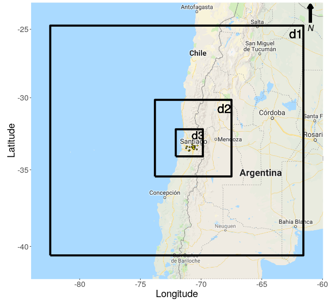
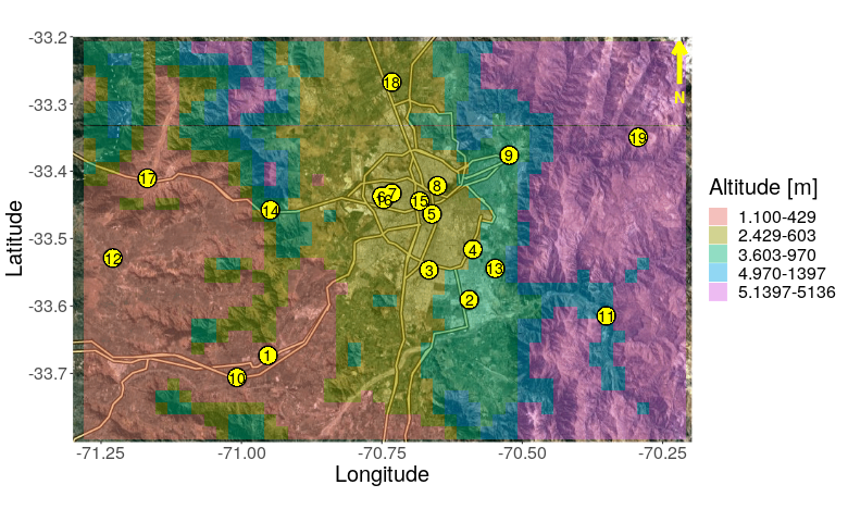
(a) (b)

Figure 1: Location maps: (a) WRF domains 1, 2, and 3; (b) domain 3 with terrain elevation (m) and location of 19 meteorological stations.

The simulations included 44 vertical levels with variable resolution, with eight levels within the first kilometer in the vertical with spacing varying between 60 and 200 m. The Final Analysis (FNL) at 0.25 deg. $\times$ 0.25 deg. horizontal resolution provided the initial and boundary conditions every 6 hours, and an analysis nudging was implemented in the outer domain (d1) to provide better boundary conditions during the simulation period. Table 1 describes the parametrizations used on each simulation.

Table 1: Description of the parametrizations set used on each of the nine members.

Member	LSM	Surface	PBL	Cumulus	Microph.	LW Rad	SW rad
1	Noah	MYNN	MYNN	Kain-F	WSM3	RRTMG	RRTMG
2	Noah	MYJ	MYJ	Kain-F	WSM3	RRTMG	RRTMG
3	Noah	YSU	YSU	Kain-F	WSM3	RRTMG	RRTMG
4	Pleim-Xiu	MYJ	MYJ	Kain-F	WSM3	RRTMG	RRTMG
5	Pleim-Xiu	YSU	YSU	Kain-F	WSM3	RRTMG	RRTMG
6	5-layer	MYJ	MYJ	Kain-F	WSM3	RRTMG	RRTMG
7	5-layer	YSU	YSU	Kain-F	WSM3	RRTMG	RRTMG
8	5-layer	MYNN	MYNN	Kain-F	WSM3	RRTMG	RRTMG
9	Pleim-Xiu	MYNN	MYNN	Kain-F	WSM3	RRTMG	RRTMG
LSM: Land-surface model, PBL: planetary boundary layer scheme,
Microph: microphysics scheme, Cumulus: represents the convective scheme,
LW Rad and SW Rad represent the longwave and shortwave radiation schemes.

The members differ each other in the applied planetary boundary layer (PBL) and land-surface model (LSM) parametrizations. We use the Mellor-Yamada-Janjic (MYJ; Janjić,, 1994), Yonsei University (YSU; Hong et al.,, 2006) and Mellor-Yamada Nakanishi and Ninno 2.5 level (MYNN; Nakanishi and Niino,, 2006) schemes to represent the PBL and surface layer processes. The Land-surface processes are represented by the 5-layer (Dudhia,, 1996), Noah (Chen and Dudhia,, 2001) and Pleim-Xiu (Pleim and Xiu,, 2003) schemes. The rest of the parametrizations are kept the same in all simulations. We use the Kain-Fritsch (Kain-F; Kain,, 2004) cumulus parametrization, the Rapid Radiative Transfer Model (RRTMG; Iacono et al.,, 2005) to represent the longwave and shortwave radiative processes and the WRF single-moment 3-class(WSM3; Hong et al.,, 2004) scheme to represent convective processes.

2.2 Station observations

Surface temperature observations (K) every 3 hours for the period between 1 October 2017 and 30 January 2018 were obtained from the Dirección Meteorológica de Chile (DMC, Government agency responsible for managing the meteorological data and providing operational weather forecasts in the country, available online at http://www.meteochile.gob), and from the National System for Air Quality (Environmental Ministry, see https://sinca.mma.gob.cl/) for 19 meteorological stations described in Table 2 (see also Figure 1b).

Table 2: Geographical coordinates in decimal degrees and altitude of monitoring stations.

No.	Station	Longitude	Latitude	Altitude (m)
1	Talagante	-70.9528	-33.6733	390
2	Puente Alto	-70.5944	-33.5908	670
3	El Bosque	-70.6660	-33.5465	580
4	La Florida	-70.5881	-33.5161	601
5	Parque O’Higgins	-70.6606	-33.4637	549
6	Pudahuel	-70.7501	-33.4373	494
7	Cerro Navia	-70.7319	-33.4326	500
8	Independencia	-70.6511	-33.4217	560
9	Las Condes	-70.5232	-33.3763	798
10	El Paico	-71.0079	-33.7059	275
11	San José Guayacán	-70.3505	-33.6148	928
12	Chorombo Hacienda	-71.2291	-33.5289	145
13	Aguas Andinas	-70.5483	-33.5445	665
14	Lo Prado	-70.9485	-33.4575	1068
15	Quinta Normal	-70.6827	-33.4445	534
16	San Pablo	-70.7466	-33.4417	490
17	Curacaví	-71.1676	-33.4106	208
18	Lo Pinto	-70.7321	-33.2675	512
19	El Colorado	-70.2935	-33.3495	2750

We remark that Las Condes (9), La Florida (4) and Chorombo Hacienda (12) stations have more than 25 % of missing values.

2.3 Predictive performance of the raw ensemble

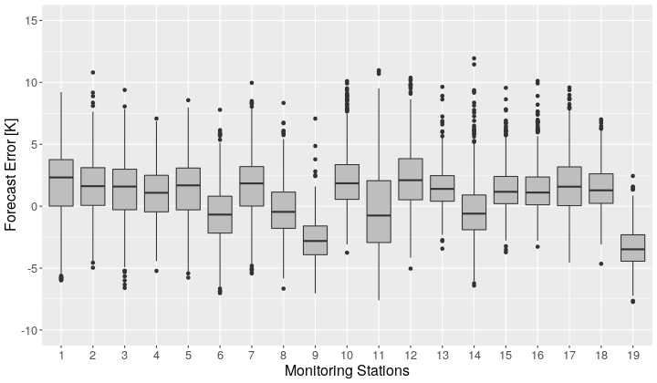
Figure 2: Forecast error of the ensemble mean for different monitoring stations.

As the altitude description of stations in Table 2 and Figure 1b show, the topography within the ensemble domain of study is very complex causing difficulties to obtain reliable forecasts. Figure 2 provides box-plots of the forecast errors of the ensemble means for the different stations. It shows that the raw ensemble systematically underestimates temperature at stations located at higher altitudes (stations 9, 11, 14 and 19). This fact should be obviously taken into account during the calibration process. A number of studies have found cold biases in near-surface temperature forecasts with the WRF model in different mountainous regions in Chile and other parts of the world using similar options for PBL and LSM schemes as those used in this study (Ruiz et al.,, 2010; Marín et al.,, 2013; Massey et al.,, 2016; González and Garreaud,, 2017). The temperature underestimation may be the result of misrepresentations in the real orography or the near-surface moisture in the model (Massey et al.,, 2016). There is also some variation in the performance of the different ensemble members (Figure 3a) and the forecast hour has influence on the forecast error (Figure 3b), too. According to Figure 3a ensemble members 7 and 8 underperform the other 7 forecasts, whereas the performance of forecasts for 12 and 15 UTC also differs from the results for other forecast hours. The latter might be related to the misrepresentation of the real orography in the model. The temperature diurnal variation is strongly influenced by solar radiation, which strongly varies in sites located in complex terrain due to topographic shading and variations in slope orientations (Zhang et al.,, 2018). Therefore, the time of sunrise in those stations might be misrepresented, causing larger errors at above mentioned hours.

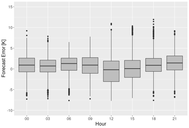
(a) (b)

Figure 3: Forecast error (a) of the different ensemble members for all dates and forecast hours; (b) of the ensemble mean for different forecast hours for all dates.

In order to get a first overview of the raw ensemble calibration, one can have a look at the verification rank histogram (Figure 4), which represents the histogram of ranks of validating observations with respect to the corresponding ensemble forecasts computed from the ranks at all locations and dates considered (see e.g. Wilks,, 2011, Section 7.7.2). In case of a proper calibration the ranks should be uniformly distributed, which is far not the case in Figure 4, calling for some form of statistical post-processing.

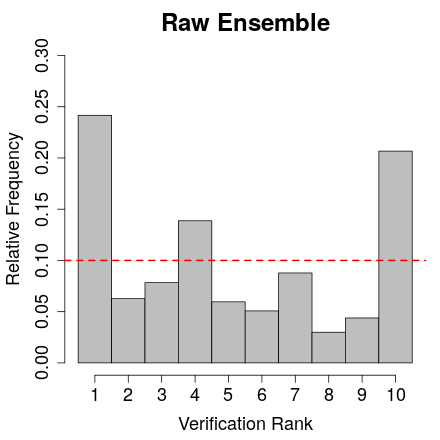
Figure 4: Verification rank histogram of raw ensemble forecasts for the period 1 October 2017 – 30 January 2018.

3 Models

As mentioned in the Introduction, normal distribution is suitable for temperature modelling, hence we make use of normal EMOS and BMA models suggested by Gneiting et al., (2005) and Raftery et al., (2005), respectively. In what follows, let $f_{1},\ldots,f_{9}$ denote the 9 ensemble members for a given location and time point.

3.1 EMOS model for temperature

The normal EMOS predictive distribution in our case has the form

$$\mathcal{N}(a_{0}+a_{1}f_{1}+\cdots+a_{9}f_{9},b_{0}+b_{1}S^{2}),\qquad\textrm{where}\qquad S^{2}:=\frac{1}{8}\sum_{k=1}^{9}(f_{k}-\bar{f})^{2},$$ (3.1)

with $\bar{f}$ denoting the ensemble mean. Location parameters $a_{0},a_{1},\ldots,a_{9}\in\mathbb{R}$ and scale parameters $b_{0},b_{1}\in\mathbb{R}$ ($a_{1},\ldots,a_{9},b_{0},b_{1}\geq 0$) are estimated by optimizing the value of a proper scoring rule (see Section 3.3), over the training data consisting of ensemble members and verifying observations from the preceding $n$ days.

3.2 BMA model for temperature

EMOS calibration is efficient in the case of unimodal distributions, however, it cannot provide an appropriate model for weather variables following distributions with several modes. In such situations BMA modelling using mixture distributions might be of more use. The normal BMA model of Raftery et al., (2005) for calibrating temperature forecasts in our case results in the predictive PDF

$$p(x|f_{1},\ldots,f_{9}):=\sum_{k=1}^{9}\omega_{k}\frac{1}{\sigma}\varphi\Big{(}\frac{x-\beta_{0,k}-\beta_{1,k}f_{k}}{\sigma}\Big{)},$$ (3.2)

where $\varphi$ denotes the PDF of the standard normal distribution. Here the weights $\omega_{k}$ reflect to the relative performance of each ensemble member $f_{k}$ during the training period and note that they should form a probability distribution, that is $\sum_{k=1}^{9}\omega_{k}=1$, $\omega_{k}\geq 0$. The linear form $\beta_{0,k}+\beta_{1,k}f_{k}$ of the mean of each component PDF is responsible for the bias correction, however, one might also consider cases $\beta_{1,k}=1$ (additive bias correction) and $\beta_{0,k}=0,\ \beta_{1,k}=1$ (no bias correction). The latter two approaches might be helpful in situations where the raw ensemble is unbiased and additional bias correction might introduce unnecessary extra errors (see e.g. Baran et al.,, 2014)

Similar to the EMOS approach, location parameters $\beta_{0,k},\beta_{1,k}$, weights $\omega_{k},\ k=1,\ldots,9$, and scale $\sigma$ are estimated using appropriate training data. Location parameters are obtained from regressing the validating observations on the ensemble members, whereas weights and scale are estimated using a maximum likelihood approach where the likelihood function is maximized with the help of the EM algorithm for mixtures (see e.g. McLachlan and Krishnan,, 1997). Note that BMA modelling is performed with the help of the ensembleBMA R package (Fraley et al.,, 2011).

3.3 Verification scores

The aim of statistical post-processing is to maximize the sharpness of the predictive distribution subject to calibration (Gneiting et al.,, 2007), where the former refers to the concentration of the forecast distribution, whereas the latter to the consistency between predicted probabilities and observed relative frequencies. These goals can be addressed simultaneously with the help of scoring rules (Gneiting and Raftery,, 2007) assigning numerical values to pairs of forecast distributions and validating observations. One of the most widely used proper scoring rule in atmospheric sciences is the continuous ranked probability score (CRPS; Gneiting and Raftery,, 2007). For a predictive cumulative distribution function (CDF) $F(y)$ and observation $x$ the CRPS is defined as

$$\mathop{\hbox{\rm CRPS}}\big{(}F,x\big{)}:=\int_{-\infty}^{\infty}\big{(}F(y)-{\mathbbm{1}}_{\{y\geq x\}}\big{)}^{2}{\mathrm{d}}y={\mathsf{E}}|X-x|-\frac{1}{2}{\mathsf{E}}|X-X^{\prime}|,$$ (3.3)

where ${\mathbbm{1}}_{H}$ denotes the indicator of a set $H$, while $X$ and $X^{\prime}$ are independent random variables with CDF $F$ and finite first moment. Note that the CRPS can be expressed in the same units as the observation and it is a negatively oriented scoring rule, that is the smaller the better.

Further, calibration of a predictive distribution can be investigated using the coverage of the $(1-\alpha)100\,\%,\ \alpha\in(0,1),$ central prediction interval. By coverage we mean the proportion of validating observations located between the lower and upper $\alpha/2$ quantiles of the predictive CDF and level $\alpha$ should be chosen to match the nominal coverage of the raw ensemble, which is $80\,\%$ for the 9 member ensemble at hand. As the coverage of a calibrated predictive distribution should be around $(1-\alpha)100\,\%$, the suggested choice of $\alpha$ allows direct comparisons with the raw ensemble.

The improvement in calibration with respect to the raw ensemble can also be demonstrated with the help of the probability integral transform (PIT) histograms (Wilks,, 2011). The PIT is the value of the predictive CDF evaluated at the validating observation and in case of proper calibration it should follow a uniform law on $[0,1]$ interval. Hence the PIT histogram is the continuous counterpart of the verification rank histogram of the raw ensemble.

Finally, a predictive performance of point forecasts is evaluated with the help of mean absolute error (MAE) and root mean squared error (RMSE). Note, that the former is optimal for the median, whereas the latter is for the mean (Gneiting,, 2011; Pinson and Hagedorn,, 2012).

3.4 Training data

The choice of appropriate training data is essential for estimating the parameters of the EMOS and BMA models given by (3.1) and (3.2). In general, rolling training periods are applied; however, there are two main approaches to choosing forecast cases for training (Thorarinsdottir and Gneiting,, 2010). In the local approach parameters for a given station are estimated from the data of that particular station only. This approach usually results in a very good model fit, provided the training period is long enough to avoid numerical issues in parameter estimation (see e.g. Hemri et al.,, 2014). In contrast, regional EMOS and BMA estimate parameters using all available forecast cases from the training period, thus all stations in the forecast domain share the same set of parameters. In this way one can use shorter training periods, but the regional approach is not suitable for large heterogeneous domains, e.g. for global forecasts. Recently Lerch and Baran, (2017) proposed a third, semi-local approach, which combines the advantages of local and regional forecasting. Training data for a given station are augmented with data for stations with similar characteristics, e.g. by clustering the stations using feature vectors determined by station climatology and/or ensemble forecast errors during the training period. Within a given cluster a regional parameter estimation is performed, but note that clusters may vary as the training window slides (for more details see Lerch and Baran,, 2017). Finally, one can also perform an expert clustering of the monitoring stations based on their location or other covariates, and estimate the parameters within clusters regionally.

4 Results

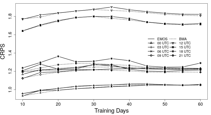
Figure 5: Mean CRPS of EMOS and BMA predictive distributions for the period 30 November 2017 – 30 January 2018.

In order to exclude the natural daily variation in temperature, EMOS and BMA calibration of WRF ensemble forecasts described in Section 2.1 is performed separately for each forecast hour. Since the ensemble has 9 members, EMOS post-processing requires a total of 11 parameters to be estimated, whereas for BMA the number of free parameters is 27. The data set at hand covers only 122 calendar days which for both approaches makes the local estimation of parameters impossible. Regional estimation also requires at least a 6 day training period (114 forecast cases) for EMOS and at least a 15 day training (285 forecast cases) for BMA in order to have at least 10 forecast cases for each parameter.

Table 3: CRPS of probabilistic, RMSE of mean and MAE of median forecasts, and coverage of 80 % central prediction intervals.

Scores	Models	Forecast hour (UTC)								Overall
		00	03	06	09	12	15	18	21
	Ens	1.728	1.570	1.743	1.773	2.135	1.839	1.604	1.764	1.769
CRPS	EMOS	1.186	1.012	1.017	1.219	1.775	1.672	1.309	1.260	1.306
(K)	EMOS-C	1.105	0.955	0.992	1.218	1.686	1.505	1.163	1.180	1.225
	BMA	1.197	1.018	1.019	1.221	1.778	1.668	1.247	1.254	1.299
	Ens	2.794	2.569	2.817	2.835	3.265	3.297	3.041	3.019	2.963
RMSE	EMOS	2.092	1.791	1.808	2.156	3.121	2.988	2.418	2.228	2.370
(K)	EMOS-C	1.951	1.692	1.755	2.149	2.996	2.697	2.111	2.114	2.222
	BMA	2.097	1.795	1.810	2.156	3.118	2.959	2.236	2.212	2.342
	Ens	2.255	1.903	2.153	2.312	2.712	2.496	2.244	2.500	2.321
MAE	EMOS	1.683	1.417	1.437	1.729	2.557	2.367	1.828	1.788	1.850
(K)	EMOS-C	1.571	1.340	1.393	1.727	2.415	2.104	1.592	1.659	1.725
	BMA	1.693	1.420	1.443	1.732	2.533	2.357	1.745	1.778	1.837
	Ens	51.15	58.14	57.05	61.14	40.46	69.04	80.98	67.18	60.63
Cover.	EMOS	75.63	75.56	76.36	76.66	77.30	77.59	75.37	78.36	76.60
(%)	EMOS-C	76.40	74.25	75.53	75.29	76.86	73.84	72.62	76.88	75.21
	BMA	74.42	76.33	77.29	75.12	74.49	75.61	76.09	76.44	75.72

We determine the length of the optimal training period by calibrating the ensemble forecasts using training periods of length $10,15,\ldots,60$ days and comparing the predictive performance on the verification period 30 November 2017 – 30 January 2018 (62 calendar days). Figure 5 shows the mean CRPS values of EMOS and BMA predictive distributions as functions of the training period length for all forecast hours. Both models have the best predictive performance at forecast hours 3 and 6 UTC, provide a bit higher CRPS values for 0, 9, 18 and 21 UTC, whereas the worse forecast skill corresponds to 12 and 15 UTC. However, these results are partially in line with Figure 3b and might be explained by the differences in accuracy of ensemble forecasts for different periods of a day. Note that the curves have their minima at day 10 and except the ones corresponding to 12 and 15 UTC do not show much variability. MAE and RMSE values of EMOS and BMA median and mean forecasts (not reported), respectively, are very consistent to the CRPS and do not change the overall picture. As in general one prefers shorter training periods, but has to keep in mind also the minimum number of forecast cases for parameter estimation, a training period of length 15 or 20 days should be selected. Finally, a 20 day training period is chosen for calibrating the WRF forecasts as it might also be appropriate for semi-local estimation of EMOS parameters using 2 or 3 clusters of observation stations. In this way the predictive performance of EMOS and BMA post-processed forecasts can be tested on temperature data from the period between 21 October 2017 and 30 January 2018 (102 calendar days).

Besides regional estimation of BMA and EMOS parameters, clustering based semi-local EMOS parameter estimation is also tested with 2 and 3 clusters and 24 features. Half of the features are obtained as equidistant quantiles of the climatological CDF, whereas the other half as equidistant quantiles of the empirical CDF of the forecast error of the ensemble mean over the training period (Lerch and Baran,, 2017). However, this approach often produces very unbalanced cluster sizes even for two clusters. In almost 28 % of the cases, station 19 alone forms a separate cluster, whereas the other cluster consists of the remaining stations. In particular, for 18 UTC this was the case on 76 out of 102 days in the training period. This uneven clustering is in line with the bad ensemble forecast skill at station 19 (Figure 2). Having a single station in a cluster means local parameter estimation for that particular station resulting in numerical issues in the optimization procedure.

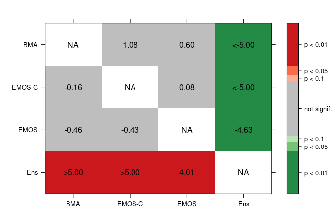
Figure 6: Values of the test statistics of the DM test for equal predictive performance based on the CRPS (upper triangle) and AE of the median forecast (lower triangle). Negative/positive values indicate a superior predictive performance of the forecast given in the row/column label, whereas green/red background indicates significant differences.

Instead of grouping the stations dynamically based on feature vectors, one might try some form of expert clustering and for the ensemble domain at hand (see Figure 1b), altitude might be a reasonable covariate. The chosen altitude regions resulting in 3 clusters are: under 400 m (stations 1, 10, 12, 17); between 400 m and 750 m (stations 2, 3, 4, 5, 6, 7, 8, 13, 15, 16, 18); above 750 m (stations 9, 11, 14, 19). Note that at stations in the third cluster, WRF forecasts systematically underestimate temperature (Figure 2).

  

  

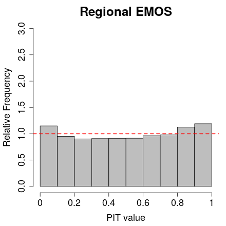
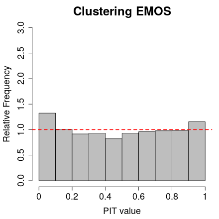
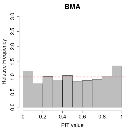
Figure 7: Verification rank histogram of the raw ensemble and PIT histograms of post-processed forecasts for the period 21 October 2017 – 30 January 2018.

In this way for post-processing ensemble forecasts we consider BMA and EMOS models with regional parameter estimation and EMOS model with clustering (EMOS-C) using a 20 day rolling training period. Table 3 shows the mean CRPS of probabilistic, the RMSE of mean and the MAE of median forecasts and the coverage of 80 % central prediction intervals separately for the different forecast hours and for the overall verification period. Note that all post-processing approaches outperform the raw ensemble in terms of all scores for all forecast hours but the coverage at 18 UTC; however, even for that forecast hour, the values are not far from the nominal 80 %. From the three competing post-processing approaches clustering based EMOS shows the best predictive performance followed by the BMA and regional EMOS. However, the differences between the scores of the three post-processing approaches are minor.

The statistical significance of differences between overall mean CRPS and MAE values is investigated with the help of two-sided Diebold-Mariano (DM; Diebold and Mariano,, 1995) tests of equal predictive performance, as this test takes into account temporal dependence (for details of application see e.g. Baran and Lerch,, 2018). Figure 6 shows the values of the DM test statistics based on the CRPS and the absolute error (AE) of median for all pairwise comparisons of forecasts. All calibration methods result in significant improvement compared to the raw ensemble; however, the forecast skill of the three post-processing approaches does not differ significantly. This means that for the WRF forecasts at hand, the use of a more complex model for calibration with many parameters does not necessary pay off. One should use a more simple approach instead and possibly group the stations in a careful way.

Table 4: p-values of Kolmogorov–Smirnov tests for uniformity of PIT values. Average of 1000 random samples of sizes 1000 each.

Model	EMOS	EMOS-C	BMA
Mean $p$-value	0.119	0.104	0.058

The same conclusions can be drawn from the overall PIT histograms plotted in Figure 7. The improvement in calibration compared to the raw ensemble is obvious; however, all three PIT histograms are slightly U-shaped indicating a very small underdispersion (see also the overall coverage values of Table 3). Unfortunately, the Kolmogorov–Smirnov test rejects the uniformity of PIT values in all three cases; however, this is the consequence of numerical problems resulted by the very large sample size (14566 valid forecast cases), see e.g. Baran and Lerch, (2015). The mean $p$-values of 1000 samples from PIT of sizes 1000 each given given in Table 4, nicely reflect to the shapes of the PIT histograms of Figure 7.

5 Conclusions

Various statistical post-processing methods are applied to 3 hourly ensemble forecasts of surface temperature for Santiago de Chile produced by separate runs of the WRF model with 9 different configurations. The one day ahead predictions for different forecast hours are treated separately. The predictive performance of EMOS and BMA models with regional parameter estimation using a 20 day training period is investigated. This optimal length of the training period is a result of a detailed data analysis. Besides the regional models, the forecast skill of an EMOS approach with parameter estimation based on clustering the observation stations is also tested. Compared to the raw ensemble, all post-processing methods for all forecast hours result in a significant decrease in CRPS values of probabilistic forecasts and MAE and RMSE values of point forecasts. In addition, they also yield a substantial improvement in calibration. From the competing calibration approaches the clustering based EMOS produces the smallest score values for all forecast hours; however, the differences in overall mean CRPS and MAE of post-processing models are not significant. We therefore conclude that post-processing of WRF ensemble forecasts for temperature significantly improves the calibration of probabilistic and the accuracy of point forecasts. However, there is still room for improvement, by considering models including spatial dependence via state of the art approaches such as Markovian EMOS (Möller et al.,, 2015) or ensemble copula coupling (Schefzik, 2016a, ; Schefzik, 2016b, ).

Acknowledgments.  Mailiu Diáz is grateful for the support of the National Commission for Scientific and Technological Research (CONICYT) of Chile under Grant No. 21150227. Sándor Baran acknowledges the support of the János Bolyai Research Scholarship of the Hungarian Academy of Sciences and the National Research, Development and Innovation Office under Grant No. NN125679. Orietta Nicolis and Julio César Marín are partially supported by the Interdisciplinary Center of Atmospheric and Astro-Statistical Studies. Powered@NLHPC: This research was partially supported by the supercomputing infrastructure of the National Laboratory for High Performing Computer (NLHPC) (ECM-02).

References

- Baran, (2014) Baran, S. (2014) Probabilistic wind speed forecasting using Bayesian model averaging with truncated normal components. Computational Statistics and Data Analysis 75, 227–238.
- Baran et al., (2014) Baran, S., Horányi, A. and Nemoda, D. (2014) Probabilistic temperature forecasting with statistical calibration in Hungary. Meteorology and Atmospheric Physics 124, 129–142.
- Baran and Lerch, (2015) Baran, S. and Lerch, S. (2015) Log-normal distribution based EMOS models for probabilistic wind speed forecasting. Quarterly Journal of the Royal Meteorological Society 141, 2289–2299.
- Baran and Lerch, (2018) Baran, S. and Lerch, S. (2018) Combining predictive distributions for statistical post-processing of ensemble forecasts. International Journal of Forecasting 34, 477–496.
- Baran and Nemoda, (2016) Baran, S. and Nemoda, D. (2016) Censored and shifted gamma distribution based EMOS model for probabilistic quantitative precipitation forecasting. Environmetrics 27, 280–292.
- Buizza et al., (2005) Buizza, R., Houtekamer, P. L., Toth, Z., Pellerin, G., Wei, M. and Zhu, Y. (2005) A comparison of the ECMWF, MSC, and NCEP global ensemble prediction systems. Monthly Weather Review 133, 1076–1097.
- Burger et al., (2018) Burger, F., Brock, B. and Montecinos, A. (2018) Seasonal and elevational contrasts in temperature trends in Central Chile between 1979 and 2015. Global and Planetary Change 162, 136–147.
- Chen and Dudhia, (2001) Chen, F. and Dudhia, J. (2001) Coupling an advanced land surface-hydrology model with the Penn State-NCAR MM5 Modeling System. Part I: Model implementation and sensitivity. Monthly Weather Review 129, 569–585.
- Cortés and Curé, (2011) Cortés, L. and Curé, M. (2011) Validation of the vertical profiles of three meteorological models using radiosondes from Antofagasta, Paranal and Llano de Chajnantor. In Curé, M., Otárola, A., Marín, J. and Sarazin, M. (eds.) Astronomical Site Testing Data in Chile. Revista Mexicana de Astronomía y Astrofísica (Serie de Conferencias) 41, pp. 64–67.
- Diebold and Mariano, (1995) Diebold F. X. and Mariano, R. S. (1995) Comparing predictive accuracy. Journal of Business & Economic Statistics 13, 253–263.
- Dudhia, (1996) Dudhia, J. (1996) A multi-layer soil temperature model for MM5. Sixth PSU/NCAR Mesoscale Model Users’ Workshop, Boulder, 22–24 July 1996, pp. 49–50.
- Fraley et al., (2011) Fraley, C., Raftery, A. E., Gneiting, T., Sloughter, J. M. and Berrocal, V. J. (2011) Probabilistic weather forecasting in R. The R Journal 3, 55–63.
- Gebhardt et al., (2011) Gebhardt, C., Theis, S. E., Paulat, M. and Ben Bouallègue, Z. (2011) Uncertainties in COSMO-DE precipitation forecasts introduced by model perturbations and variation of lateral boundaries. Atmospheric Research 100, 168–177.
- Gneiting, (2011) Gneiting, T. (2011) Making and evaluating point forecasts. Journal of the American Statistical Association 106, 746–762.
- Gneiting et al., (2007) Gneiting, T., Balabdaoui, F. and Raftery, A. E. (2007) Probabilistic forecasts, calibration and sharpness. Journal of the Royal Statistical Society: Series B 69, 243–268.
- Gneiting and Raftery, (2007) Gneiting, T. and Raftery, A. E. (2007) Strictly proper scoring rules, prediction and estimation. Journal of the American Statistical Association 102, 359–378.
- Gneiting et al., (2005) Gneiting, T., Raftery, A. E., Westveld, A. H. and Goldman, T. (2005) Calibrated probabilistic forecasting using ensemble model output statistics and minimum CRPS estimation. Monthly Weather Review 133, 1098–1118.
- González and Garreaud, (2017) González, S. and Garreaud, R. (2017) Spatial variability of near-surface temperature over the coastal mountains in southern Chile (38∘S) Meteorology and Atmospheric Physics, https://doi.org/10.1007/s00703-017-0555-4.
- Hemri et al., (2014) Hemri, S., Scheuerer, M., Pappenberger, F., Bogner, K. and Haiden, T. (2014) Trends in the predictive performance of raw ensemble weather forecasts. Geophysical Research Letters 41, 9197–9205.
- Hong et al., (2004) Hong, S.-Y., Dudhia, J. and Chen, S.-H. (2004) A revised approach to ice microphysical processes for the bulk parameterization of clouds and precipitation. Monthly Weather Review 132, 103–120.
- Hong et al., (2006) Hong, S.-Y., Noh, Y. and Dudhia, J. (2006) A new vertical diffusion package with an explicit treatment of entrainment processes. Monthly Weather Review 134, 2318–2341.
- Iacono et al., (2005) Iacono, M. J., Delamere J. S., Mlawer, E. J., Shephard, M. W., Clough, S. A. and Collins, W. D. (2005) Radiative forcing by long-lived greenhouse gases: Calculations with the AER radiative transfer models. Journal of Geophysical Research: Atmospheres 113, D13103.
- Janjić, (1994) Janjić, Z. I. (1994) The Step-Mountain Eta Coordinate Model: further developments of the convection, viscous sublayer, and turbulence closure schemes. Monthly Weather Review 122, 927–945.
- Kain, (2004) Kain, J. S. (2004) The Kain-Fritsch convective parameterization: an update. Journal of Applied Meteorology 43, 170–181.
- Leith, (1974) Leith, C. E. (1974) Theoretical skill of Monte-Carlo forecasts. Monthly Weather Review 102, 409–418.
- Lerch and Baran, (2017) Lerch, S. and Baran, S. (2017) Similarity-based semi-local estimation of EMOS models. Journal of the Royal Statistical Society: Series C 66, 29–51.
- Leutbecher and Palmer, (2008) Leutbecher, M. and Palmer, T. N. (2008) Ensemble forecasting. Journal of Computational Physics 227, 3515–3539.
- Marín et al., (2013) Marín, J. C., Pozo, D., Mlawer, E., Turner, D. and Curé, M. (2013) Dynamics of local circulations in mountainous terrain during the RHUBC-II project. Monthly Weather Review 141, 3641–3656.
- Massey et al., (2016) Massey, J. D., Steenburgh, W. J., Knievel, J. C. and Cheng, W. Y. Y. (2016) Regional soil moisture biases and their influence on WRF Model temperature forecasts over the Intermountain West. Weather and Forecasting 31, 197–216,
- McLachlan and Krishnan, (1997) McLachlan, G. J. and Krishnan, T. (1997) The EM Algorithm and Extensions. Wiley, New York.
- Molteni et al., (1996) Molteni, F., Buizza, R., Palmer, T. N. and Petroliagis, T. (1996) The ECMWF ensemble prediction system: Methodology and validation. Quarterly Journal of the Royal Meteorological Society 122, 73–119.
- Möller et al., (2015) Möller, A., Thorarinsdottir, T. L., Lenkoski, A. and Gneiting, T. (2015) Spatially adaptive, Bayesian estimation for probabilistic temperature forecasts. arXiv:1507.05066.
- Nakanishi and Niino, (2006) Nakanishi, M. and Niino, H. (2006) An improved Mellor–Yamada Level-3 Model: its numerical stability and application to a regional prediction of advection fog. Boundary-Layer Meteorology 119, 397–407.
- Pinson and Hagedorn, (2012) Pinson, P. and Hagedorn, R. (2012) Verification of the ECMWF ensemble forecasts of wind speed against analyses and observations. Meteorological Applications 19, 484–500.
- Pleim and Xiu, (2003) Pleim, J. E. and Xiu, A. (2003) Development of a land surface model. Part II: Data assimilation. Journal of Applied Meteorology 42, 1811-1822.
- Powers et al., (2017) Powers, J. G., Klemp, J. G., Skamarock, W. S., Davis, C. A., Dudhia, J., Gill, D. O., Coen, J. L., Gochis, D. J., Ahmadov, R., Peckham, S. E., Grell, G. A., Michalakes, J., Trahan, S., Benjamin, S. G., Alexander, C. R., Dimego, G. J., Wang, W., Schwartz, C. S., Romine, G. S., Liu, Z., Snyder, C., Chen, F., Barlage, M. J., Yu, W. and Duda, M. G. (2017) The Weather Research and Forecasting Model: overview, system efforts, and future directions. Bulletin of the American Meteorological Society 98, 1717–1737.
- Pozo et al., (2016) Pozo, D., Marín, J. C., Illanes, L., Curé, M. and Rabanus, D. (2016) Validation of WRF forecasts for the Chajnantor region. Monthly Notices of the Royal Astronomical Society 459, 419–426.
- Raftery et al., (2005) Raftery, A. E., Gneiting, T., Balabdaoui, F. and Polakowski, M. (2005) Using Bayesian model averaging to calibrate forecast ensembles. Monthly Weather Review 133, 1155–1174.
- Ruiz et al., (2010) Ruiz, J. J., Saulo, C. and Nogues-Paegle, J. (2010) WRF model sensitivity to choice of parameterization over South America: Validation against surface variables. Monthly Weather Review 138, 3342–3355.
- Saide et al., (2011) Saide, P. E., Carmichael, G. R., Spak, S. N., Gallardo, L., Osses, A. E., Mena-Carrasco, M. A. and Pagowski, M. (2011) Forecasting urban PM10 and PM2.5 pollution episodes in very stable nocturnal conditions and complex terrain using WRF–Chem CO tracer model. Atmospheric Environment 45, 2769–2780.
- (41) Schefzik, R. (2016a) A similarity-based implementation of the Schaake shuffle. Monthly Weather Review 144, 1909–1921.
- (42) Schefzik, R. (2016b) Combining parametric low-dimensional ensemble postprocessing with reordering methods. Quarterly Journal of the Royal Meteorological Society 142, 2463–2477.
- Scheuerer, (2014) Scheuerer, M. (2014) Probabilistic quantitative precipitation forecasting using ensemble model output statistics. Quarterly Journal of the Royal Meteorological Society 140, 1086–1096.
- Scheuerer and Hamill, (2015) Scheuerer, M. and Hamill, T. M. (2015) Statistical post-processing of ensemble precipitation forecasts by fitting censored, shifted gamma distributions. Monthly Weather Review 143, 4578–4596.
- Skamarock et al., (2008) Skamarock, W. C., Klemp, J. B., Dudhia, J., Gill, D. O., Barker, D. M., Duda, M., Huang, X. Y., Wang, W. and Powers, J .G. (2008). A description of the Advanced Research WRF Version 3. NCAR Technical Note, NCAR/TN–475+ST.
- Sloughter et al., (2010) Sloughter, J. M., Gneiting, T. and Raftery, A. E. (2010) Probabilistic wind speed forecasting using ensembles and Bayesian model averaging. Journal of the American Statistical Association 105, 25–37.
- Sloughter et al., (2007) Sloughter, J. M., Raftery, A. E., Gneiting, T. and Fraley, C. (2007) Probabilistic quantitative precipitation forecasting using Bayesian model averaging. Monthly Weather Review 135, 3209–3220.
- Thorarinsdottir and Gneiting, (2010) Thorarinsdottir, T. L. and Gneiting, T. (2010) Probabilistic forecasts of wind speed: ensemble model output statistics by using heteroscedastic censored regression. Journal of the Royal Statistical Society: Series A 173, 371–388.
- Wannitsem et al., (2018) Wannitsem, S., Wilks, D. S. and Messner, J. W. (eds.) (2018) Statistical Postprocessing of Ensemble Forecasts, Elsevier, Amsterdam.
- Williams et al., (2014) Williams, R. M., Ferro, C. A. T. and Kwasniok F (2014) A comparison of ensemble post-processing methods for extreme events. Quarterly Journal of the Royal Meteorological Society 140, 1112–1120.
- Wilks, (2011) Wilks, D. S. (2011) Statistical Methods in the Atmospheric Sciences (3rd ed.). Elsevier, Amsterdam.
- Zhang et al., (2018) Zhang, Y. L., Li, X., Cheng, G. D., Jin, H. J., Yang, D. W., Flerchinger, G. N., Chang, X. L., Wang, X. and Liang, J. (2018) Influences of topographic shadows on the thermal and hydrological processes in a cold region mountainous watershed in northwest China. Journal of Advances in Modeling Earth Systems 10, 1439–1457.