Polarization observables in $e^{+}e^{-}$ annihilation to a baryon-antibaryon pair

Abstract

Using the helicity formalism of Jacob and Wick we derive spin density matrices of baryon antibaryon pairs produced in $e^{+}e^{-}$ annihilation. We consider the production of pairs with spins $1/2+\overline{1/2}$, $1/2+\overline{3/2}$ (+c.c.) and $3/2+\overline{3/2}$. We provide modular expressions to include chains of weak hadronic two-body decays of the produced hyperons. The expressions are suitable for the analysis of high statistics data from $J/\psi$ and $\psi(2S)$ decays at $e^{+}e^{-}$ colliders, by fits to the fully differential angular distributions of the measured particles. We illustrate the method by examples, such as the inclusive measurement of the $e^{+}e^{-}\to\psi(2S)\to\Omega^{-}\bar{\Omega}^{+}$ process where one decay chain $\Omega^{-}\to\Lambda K^{-}$ followed by $\Lambda\to p\pi^{-}$ is considered. Finally we show that the inclusive angular distributions can be used to test spin assignment of the produced baryons.

I Introduction

Charmonia are excellent sources of spin entangled hyperon antihyperon pairs. In particular the states $J/\psi$ or $\psi(2S)$, which carry $J^{PC}=1^{--}$, are directly produced at electron positron colliders. They are perfectly suited for precise determination of hyperon decay parameters and searches for $CP$ symmetry violation in the baryon sector.

Recent, unexpected observation of polarization in $e^{+}e^{-}\to J/\psi\to\Lambda\bar{\Lambda}$ at BESIII Ablikim et al. (2018) opens up new perspectives for such measurements. The polarization allows simultaneous determination of the $\Lambda$ and $\bar{\Lambda}$ decay asymmetries from the events, in which all decay products are measured. Of major importance is the new BESIII result for the $\Lambda\to p\pi^{-}$ asymmetry parameter of $\alpha_{-}=0.750\pm 0.009\pm 0.004$. This decay is used in practically in all experiments involving $\Lambda$ for identification and for polarization determination from the measured product of the polarization and the known value of the asymmetry parameter. All these studies assume the asymmetry parameter of $0.642\pm 0.013$, the world-average value established in 1978 Bricman et al. (1978) and unchanged until the 2018 edition of Review of Particle Physics Tanabashi et al. (2018). Therefore the new BESIII value implies that all published measurements on $\Lambda/\bar{\Lambda}$ polarization are $(17\pm 3)\%$ too large. This includes e.g. values of decay asymmetries for weak decays of strange and charmed baryons into final states including $\Lambda$ such as $\Xi\to\Lambda\pi$, $\Omega^{-}\to\Lambda\pi^{-}$ etc. The BESIII analysis uses fully differential distributions derived in Ref. Fäldt and Kupść (2017) using Feynman diagrams formalism. Previous $e^{+}e^{-}\to J/\psi\to\Lambda\bar{\Lambda}$ measurements Tixier et al. (1988); Ablikim et al. (2010) used simplified and not correct expressions for the amplitudes which precluded such analysis. These expressions were derived using helicity formalism of Jacob and Wick Jacob and Wick (1959). Therefore, the important tasks is to repeat the derivation of the angular distributions to make sure the results are consistent. In addition the helicity formalism would allow to generalize the angular distributions for the higher spin states.

With a large number of collected $J/\psi$, $(1310.6\pm 7.0)\times 10^{6}$, and $\psi(2S)$, $(448.1\pm 2.9)\times 10^{6}$, at the BESIII experiment Ablikim et al. (2012, 2017a, 2013) detailed studies of such systems are now possible.

Examples of the available data samples from recent publications are given in Table 1. The branching fractions, ${\cal B}$, for the listed decay modes range between $10^{-4}$ and $10^{-3}$ and the reconstructed data samples are up to $10^{6}$ events. In addition, considering world averages of the ${\cal B}$ values for other $B_{1}\bar{B}_{2}$ decays, one can anticipate that more modes are accessible with the collected data sets (Table 2). All of the published results focus only on the determination of the branching fractions and the angular distributions of the produced hyperons.

decay mode	events			${\cal B}({\rm units}\ 10^{-4})$
$J/\psi\to\Lambda\bar{\Lambda}$$\int\limits^{M}$	$440675$	$\pm$	$670$	${19.43\pm 0.03\pm 0.33}$
$\psi(2S)\to\Lambda\bar{\Lambda}$	$31119$	$\pm$	$187$	${3.97\pm 0.02\pm 0.12}$
$J/\psi\to\Sigma^{0}\bar{\Sigma}^{0}$	$111026$	$\pm$	$335$	${11.64\pm 0.04\pm 0.23}$
$\psi(2S)\to\Sigma^{0}\bar{\Sigma}^{0}$	$6612$	$\pm$	$82$	${2.44\pm 0.03\pm 0.11}$
$J/\psi\to\Sigma(1385)^{0}\bar{\Sigma}(1385)^{0}$	$102762$	$\pm$	$852$	$10.71\pm 0.09$
$J/\psi\to\Xi^{0}\bar{\Xi}^{0}$	$134846$	$\pm$	$437$	$11.65\pm 0.04$
$\psi(2S)\to\Sigma(1385)^{0}\bar{\Sigma}(1385)^{0}$	$2214$	$\pm$	$148$	$0.69\pm 0.05$
$\psi(2S)\to\Xi^{0}\bar{\Xi}^{0}$	$10839$	$\pm$	$123$	$2.73\pm 0.03$
$J/\psi\to\Xi^{-}\bar{\Xi}^{+}$	$42811$	$\pm$	$231$	$10.40\pm 0.06$
$J/\psi\to\Sigma(1385)^{-}\bar{\Sigma}(1385)^{+}$	$42595$	$\pm$	$467$	$10.96\pm 0.12$
$J/\psi\to\Sigma(1385)^{+}\bar{\Sigma}(1385)^{-}$	$52523$	$\pm$	$596$	$12.58\pm 0.14$
$\psi(2S)\to\Xi^{-}\bar{\Xi}^{+}$	$5337$	$\pm$	$83$	$2.78\pm 0.05$
$\psi(2S)\to\Sigma(1385)^{-}\bar{\Sigma}(1385)^{+}$	$1375$	$\pm$	$98$	$0.85\pm 0.06$
$\psi(2S)\to\Sigma(1385)^{+}\bar{\Sigma}(1385)^{-}$	$1470$	$\pm$	$95$	$0.84\pm 0.05$

Table 1: Available $B_{1}\bar{B}_{2}$ data samples and the branching fractions from recent BESIII publications Ablikim et al. (2017b, c, 2016).

decay mode	${\cal B}({\rm units}\ 10^{-4}$)
$J/\psi\to\Xi(1530)^{-}\bar{\Xi}^{+}$$\int\limits^{M}$	5.9	$\pm$	1.5
$J/\psi\to\Xi(1530)^{0}\bar{\Xi}^{0}$	3.3	$\pm$	1.4
$J/\psi\to\Sigma(1385)^{-}\bar{\Sigma}^{+}$	3.1	$\pm$	0.5
$\psi(2S)\to\Omega^{-}{\bar{\Omega}}^{+}$	0.47	$\pm$	0.10

Table 2: Possible other hyperon antihyperon final states which can be studied at BESIII. The quoted branching fractions are from the Particle Data Group Tanabashi et al. (2018).

The production amplitudes of such processes are described by a limited set of form factors — complex numbers at fixed center-of-mass (CM) energy. For instance, in the case of a spin-1/2 hyperon pair there are just two such form factors. The angular distribution is described by two real numbers: one related to the ratio of the absolute values of the form factors and the other giving the relative phase. In this case, provided that there is a non-negligible phase between the form factors, one can determine the decay parameters of the produced hyperons and carry out $CP$ violation tests in the baryon sector. For the spin-1/2 hyperons with single-step decay modes (analogous to $\Lambda$), the formulas provided in Ref. Fäldt and Kupść (2017) could be used directly. However, to include other interesting cases the formalism has to be extended for states where the hyperon antihyperon pair can have a combination of spins $1/2$ and $3/2$ and for multi-step decay chains.

Several approaches are suitable to provide the amplitude for a process where the final states carry nonzero spins. We use the helicity formalism originally developed by Jacob and Wick Jacob and Wick (1959). This formalism had been used in the past for several hyperon production reactions and decays Berman and Jacob (1965); Luk (1983); Tabakin and Eisenstein (1985); Diehl III. (1990); Guglielmo (1994). However, we did not find a general and modular formulation which could be applied directly to describe high statistics exclusive data, i.e. data where momenta of all particles are measured for each event. For this purpose fully differential angular distributions are needed, to be used for event generators and for maximum likelihood fits. It is the purpose of the present paper to document the construction of such a framework.

We derive spin density matrices for $e^{+}e^{-}\to B_{1}\bar{B}_{2}$ processes where the baryon (antibaryon) can have spin $1/2$ or $3/2$. In practice we focus on the cases where all baryons have positive parity and all antibaryons have negative parity. This fits to the ground state baryons of spin $1/2$ and spin $3/2$ Tanabashi et al. (2018). The presented formalism can be applied to study decays of $J^{PC}=1^{--}$ vector mesons produced in electron positron colliders, such as $J/\psi$ or $\psi(2S)$, into $B_{1}\bar{B}_{2}$ pairs. We will also revise some misleading assumptions and formulas used in the analyses of weak decay chains within this framework.

In order to establish our notation we start with applying the helicity formalism to the well known case of $1/2+\overline{1/2}$ baryons, then we proceed to the $1/2+\overline{3/2}$ and $3/2+\overline{3/2}$ cases. We present a general formalism together with detailed expressions for the spin density matrices for the production process and for the most important decay modes.

As long as the momentum direction is not flipped, boosts do not change the helicity. Therefore in the helicity amplitude method one can disregard the boost part of the Lorentz group, which allows to obtain angular distributions without using full expressions for the spinors as required by the Feynman diagram technique. This is very convenient but comes with a disadvantage: the energy dependence of the contributing amplitudes cannot be determined and therefore not even their relative importance. Yet for fixed production energy of a two-particle system and for two-body decays of the produced states all kinematical variables, i.e. all angles, are fully covered by the helicity framework.

We would like to stress again that the basics of our formalism are not new. How to describe in principle the scattering and decays of relativistic particles with spin has been established long time ago. Yet at that time, angular averages were sufficient to account for the available data. Consequently there was no need to provide detailed formulas for the fully differential angular distributions of multi-step decay chains. It is high time to fill this gap in view of the modern high-luminosity experiments, which deliver fully differential data. Only in that way the full potential of presently running and future experiments can be exploited.

The rest of the paper is organized in the following way: In Section II we provide the general helicity framework adjusted such that it fits to commonly employed experimental analyses. In Section III we specify to the three production processes that we are interested in, i.e. combinations of spin-1/2 and/or spin-3/2 baryons and antibaryons. Section IV is devoted to the general discussion of (weak) two-body decay chains. Examples are provided in Section V. We have chosen the same examples as considered in Ref. Chen and Ping (2007). To facilitate the matching of theoretical models to experimental results we relate electromagnetic form factors to helicity amplitudes in Section VI. Further discussions are provided in Section VII.

II General framework

In general we look at the production of two unstable particles in an initial scattering reaction. Subsequently the produced particles decay in one or several steps. The general task is to deduce information about the spins and their correlations among the involved (unstable) particles. If none of the spins are measured directly, this information is encoded in the angular distributions. The angles are measured with respect to some axes, which makes it necessary to define appropriate frames of reference and cartesian coordinate systems.

The production process defines the first coordinate system; see below. For the decays it is useful to boost to the rest frame of the mother particle. Yet it is helpful to perform rotations before this boost. We will be very explicit to motivate and define these rotations.

Following the ideas of Jacob and Wick (1959); Berman and Jacob (1965) we use the helicity formalism. Here the spin quantization axis is not chosen along a fixed axis but along the flight direction of the state. The advantage is that the helicity does not change when boosting to the rest frame of this state. On the other hand, the use of angular-momentum (${\bf J}$) conservation for the production and for each decay process suggests to single out the $z$-axis, based on the convention to use ${\bf J}^{2}$ and $J_{z}$ for the characterization of states.

Following this spirit it is useful to spell out how helicity states are constructed. To motivate this construction we discuss first how one deals with changes of reference frames in experimental analyses. Afterwards we will describe how to mimic these changes on the theory side.

Experimental procedure:

Suppose one has produced a “mother” particle that decays further. One wants to change from the production frame of this state to its rest frame. Given the state’s three-momentum

$${\bf p}_{m}=p_{m}\,(\cos\phi_{m}\sin\theta_{m},\sin\phi_{m}\sin\theta_{m},\cos\theta_{m})$$ (1)

and the $z$-axis in the production frame, one possibility would be to perform a single rotation that aligns ${\bf p}_{m}$ with the $z$-axis. Subsequently one then boosts to the rest frame of the mother particle. The single rotation would be around an axis perpendicular to ${\bf p}_{m}$ and $\hat{\bf z}$. Yet when viewed as rotations around the coordinate axes this amounts to a succession of three rotations. Viewed as active rotations these are (a) a rotation around the $z$-axis by $-\phi_{m}$; (b) a rotation around the $y$-axis by $-\theta_{m}$; (c) a rotation around the $z$-axis by $+\phi_{m}$; see also Jacob and Wick (1959). In principle, however, the first two rotations are sufficient to align ${\bf p}_{m}$ with the $z$-axis. In line with the present BESIII analyses we follow this two-rotation procedure in the present work. The rotation matrix for ${\bf p}_{m}$ is given by

$$\left(\begin{array}[]{rrr}\cos\theta_{m}\cos\phi_{m}&\cos\theta_{m}\sin\phi_{m}&-\sin\theta_{m}\\ -\sin\phi_{m}&\cos\phi_{m}&0\\ \cos\phi_{m}\sin\theta_{m}&\sin\theta_{m}\sin\phi_{m}&\cos\theta_{m}\\ \end{array}\right).$$ (2)

This rotation defines in a unique way the helicity reference frame for a daughter particle. In an experimental analysis the boosts and rotations in Eq (2) are applied recursively to all decay products of a decay chain, thus defining a set of helicity variables to describe an event.

Matching amplitude:

To mimic this procedure on the theory side we construct helicity states by the inverse procedure, following essentially Berman and Jacob (1965). A one-particle state with helicity $\lambda$ and momentum ${\bf p}=p\,(\cos\phi\sin\theta,\sin\phi\sin\theta,\cos\theta)$ is constructed from a state $|p,\lambda\rangle$ that moves along the $z$-direction by

$$|p,\theta,\phi,\lambda\rangle:=R(\phi,\theta,0)|p,\lambda\rangle$$ (3)

with Jacob and Wick (1959)

$$R(\alpha,\beta,\gamma):=e^{-i\alpha J_{z}}\,e^{-i\beta J_{y}}\,e^{-i\gamma J_{z}}\,.$$ (4)

Correspondingly a two-particle state in its CM frame is given by

$$|p,\theta,\phi,\lambda_{1},\lambda_{2}\rangle:=R(\phi,\theta,0)|p,\lambda_{1},\lambda_{2}\rangle\,.$$ (5)

In practice we follow all the steps of Jacob and Wick (1959) except for the fact that we use a two-angle rotation procedure as spelled out in Eq. (3). When constructing (5) the first particle has momentum ${\bf p}=p\,(\cos\phi\sin\theta,\sin\phi\sin\theta,\cos\theta)$ and helicity $\lambda_{1}$ while the second has momentum $-{\bf p}$ and helicity $\lambda_{2}$. The most important consequence of our construction of these two-particle states is their projection on angular-momentum eigenstates Berman and Jacob (1965):

$$\begin{split}&\langle J,M,\lambda_{1}^{\prime},\lambda_{2}^{\prime}|\theta,\phi,\lambda_{1},\lambda_{2}\rangle\\ &=\sqrt{\frac{2J+1}{4\pi}}{\cal D}^{J}_{M,\lambda_{1}-\lambda_{2}}(\phi,\theta,0)\,\delta_{\lambda_{1}\lambda_{1}^{\prime}}\delta_{\lambda_{2}\lambda_{2}^{\prime}}\end{split}$$ (6)

where ${\cal D}_{m^{\prime}m}^{j}(\alpha,\beta,\gamma):=\braket{jm^{\prime}}{R(\alpha,\beta,\gamma)}{jm}$ is the Wigner D-matrix.

II.1 Production process

We turn once more to a description of the experimental analysis: The production process $e^{+}e^{-}\to B_{1}\bar{B}_{2}$, viewed in the CM frame, defines a scattering plane and therefore a coordinate system. The $z$-axis is chosen along the line of flight of the incoming positron, i.e. ${\bf\hat{z}}={\bf p}_{e^{+}}=(0,0,p_{\rm in})$, where $p_{\rm in}$ denotes the modulus of the momentum of electron and positron in the CM frame. The $y$-axis is chosen to be perpendicular to the scattering plane. One uses the direction of the baryon $B_{1}$ to define the $y$-axis:

$${\bf\hat{y}}:=\frac{{\bf p}_{e^{+}}\times{\bf p}_{B}}{|{\bf p}_{e^{+}}\times{\bf p}_{B}|}\,.$$ (7)

Finally the $x$-axis is chosen such that $x$, $y$ and $z$ adhere to the right-hand rule. Denoting the scattering angle of $B_{1}$ by $\theta_{1}$, all this implies ${\bf p}_{B}=p_{\rm out}\,(\sin\theta_{1},0,\cos\theta_{1})$. Here $p_{\rm out}$ denotes the modulus of the momentum of baryon and antibaryon in the CM frame.

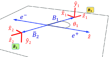
Figure 1: (color online) Orientation of the axes in baryon $B_{1}$ and antibaryon $\bar{B}_{2}$ helicity frames.

With the above definition of the CM coordinate system, the $y$ axis of the helicity frame of the baryon $B_{1}$, ${\bf\hat{y}}_{1}$ in Fig. 1, is the same as ${\bf\hat{y}}$ in Eq. (7). Therefore, for the helicity rotation matrix Eq. (2) one uses $\theta_{m}=\theta_{1}$ and $\phi_{m}=0$. Correspondingly, to transform to the helicity frame of the antibaryon $\bar{B}_{2}$ one chooses $\phi_{m}=\pi$ and $\theta_{m}=\pi-\theta_{1}$. In this way the $y$-axis, ${\bf\hat{y}}_{2}$, is equal $-{\bf\hat{y}}$. The $y$- and $z$-axes of the helicity frames of the baryon $B_{1}$ and the antibaryon $\bar{B}_{2}$ have opposite directions while it is the same direction for the $x$-axis as shown in Fig. 1.

Now we turn to the theoretical construction that goes along with the experimental analysis: Let $\lambda$ denote the initial helicity of the positron. Neglecting the mass of the electron and working within the one-photon approximation this implies that the helicity of the electron is $-\lambda$ since the photon only couples right-handed particles to left-handed antiparticles and vice versa. Since $\lambda$ can take the values $\pm 1/2$, then the helicity difference $k:=\lambda-(-\lambda)=\pm 1$.

For unpolarized initial states one sums over $\lambda$ or equivalently over $k=2\lambda$. The density matrix for the production is proportional to

$$\rho^{\lambda_{1},\lambda_{2};\lambda_{1}^{\prime},\lambda_{2}^{\prime}}_{B_{1}\bar{B}_{2}}\propto\sum\limits_{k=\pm 1}{}_{\rm o}\!\langle\theta_{1},0,\lambda_{1},\lambda_{2}|S|0,0,\lambda,-\lambda\rangle_{\rm i}\;$$

$$\phantom{\sim}\times_{\rm i}\!\!\langle 0,0,\lambda,-\lambda|S^{\dagger}|\theta_{1},0,\lambda_{1}^{\prime},\lambda_{2}^{\prime}\rangle_{\rm o}\,,$$ (8)

where we use the $\langle$bra$|$, $|$ket$\rangle$ notation with index $\rm i$ and $\rm o$ to denote in and out states, respectively. Now we evaluate the transition operator $S$:

$${}_{\rm o}\!\langle\theta_{1},0,\lambda_{1},\lambda_{2}|S|0,0,\lambda,-\lambda\rangle_{\rm i}$$

$$=\sum\limits_{J,M}{}_{\rm o}\!\langle\theta_{1},0,\lambda_{1},\lambda_{2}|JM,\lambda_{1},\lambda_{2}\rangle_{\rm o}$$

$$\times{}_{\rm o}\!\langle JM,\lambda_{1},\lambda_{2}|S|JM,\lambda,-\lambda\rangle_{\rm i}$$

$$\times{}_{\rm i}\!\langle JM,\lambda,-\lambda|0,0,\lambda,-\lambda\rangle_{\rm i}\,.$$ (9)

We have to evaluate three matrix elements. The first and the third bring in Wigner functions. The general formula is given in Eq. (6). For the transition amplitude one finds in the one-photon approximation

$${}_{\rm o}\!\langle JM,\lambda_{1},\lambda_{2}|S|JM,\lambda,-\lambda\rangle_{\rm i}$$

$$\approx{}_{\rm o}\!\langle JM,\lambda_{1},\lambda_{2}|S_{\gamma^{*}\to{\rm out}}\,S_{{\rm in}\to\gamma^{*}}|JM,\lambda,-\lambda\rangle_{\rm i}$$

$$=\delta_{J,1}\,\,A_{\lambda_{1},\lambda_{2}}\,A^{{\rm in}}_{\lambda,-\lambda}\,.$$ (10)

Here $A_{\lambda_{1},\lambda_{2}}$ denotes the transition amplitude between helicity states. Only transitions fulfilling the inequality

$$|\lambda_{1}-\lambda_{2}|\leq J=1$$ (11)

are different from zero. For a parity conserving process the amplitudes between opposite helicity states are related:

$$A_{\lambda_{1},\lambda_{2}}=\eta_{1}\eta_{2}\eta(-1)^{J-s_{1}-s_{2}}A_{-\lambda_{1},-\lambda_{2}}\,,$$ (12)

where $\eta$ is the parity of the initial state, $\eta_{1}$ and $\eta_{2}$ are the parities of the final state particles. Moreover parity symmetry of QED implies $A^{{\rm in}}_{-\lambda,\lambda}=A^{{\rm in}}_{\lambda,-\lambda}$ for the initial $e^{+}e^{-}\to\gamma^{*}$ production amplitude $A^{{\rm in}}$. Here we are not interested in the $p_{\rm in}$ dependence of the reaction and therefore we can drop $A^{{\rm in}}$. One finds

$${}_{\rm o}\!\langle\theta_{1},0,\lambda_{1},\lambda_{2}|S|0,0,\lambda,-\lambda\rangle_{\rm i}$$

$$\propto\sum\limits_{M}[{\cal D}_{M,\lambda_{1}-\lambda_{2}}^{1}(0,\theta_{1},0)]^{*}\,A_{\lambda_{1},\lambda_{2}}\,{\cal D}_{M,k}^{1}(0,0,0)$$

$$=[{\cal D}_{k,\lambda_{1}-\lambda_{2}}^{1}(0,\theta_{1},0)]^{*}\,A_{\lambda_{1},\lambda_{2}}\,.$$ (13)

We obtain for the production density matrix:

$$\rho^{\lambda_{1},\lambda_{2};\lambda_{1}^{\prime},\lambda_{2}^{\prime}}_{B_{1}\bar{B}_{2}}\propto A_{\lambda_{1},\lambda_{2}}\,A^{*}_{\lambda^{\prime}_{1},\lambda^{\prime}_{2}}\,\rho_{1}^{\lambda_{1}-\lambda_{2},\lambda^{\prime}_{1}-\lambda^{\prime}_{2}}(\theta_{1}\!)$$ (14)

with

$$\rho_{1}^{i,j}(\theta):=\sum\limits_{k=\pm 1}{\cal D}_{k,i}^{1*}(0,\theta,0)\,{\cal D}^{1}_{k,j}(0,\theta,0)\,.$$ (15)

The explicit form of the reduced density matrix $\rho_{1}$ is given by

$$\rho_{1}(\theta)=\left(\begin{array}[]{ccc}\frac{1+\cos^{2}\!\theta}{2}&-\frac{\cos\theta\sin\theta}{\sqrt{2}}&\frac{\sin^{2}\!\theta}{2}\\[5.0pt] -\frac{\cos\theta\sin\theta}{\sqrt{2}}&\sin^{2}\!\theta&\frac{\cos\theta\sin\theta}{\sqrt{2}}\\[5.0pt] \frac{\sin^{2}\!\theta}{2}&\frac{\cos\theta\sin\theta}{\sqrt{2}}&\frac{1+\cos^{2}\!\theta}{2}\\ \end{array}\right)\,.$$ (16)

We note in passing that here one could also rotate to a frame where the baryons do not lie in the $x$-$z$ plane, i.e. where they have a non-vanishing value of $\phi$. This would not change the density matrix because of the following relation:

$${\cal D}_{k,i}^{1*}(0,\theta,0)\,{\cal D}^{1}_{k,j}(0,\theta,0)={\cal D}_{k,i}^{1*}(\phi,\theta,0)\,{\cal D}^{1}_{k,j}(\phi,\theta,0)\,.$$ (17)

This also points to the core difference with all previous helicity amplitude calculations of the $e^{+}e^{-}\to B_{1}\bar{B}_{2}$ process starting from Ref. Tixier et al. (1988). All they obtain the initial $\rho_{1}$ density matrix which is dependent on $\phi$. This is an unphysical result for transversely unpolarized electron and positron beams due to the rotation symmetry with respect to the ${\bf\hat{z}}$ axis. The unwanted $\phi$ dependence is then eliminated by an arbitrary integration over the $\phi$ variable. The result is a diagonal density matrix and all interference terms between heicity amplitudes of the produced baryons cancel. We can reproduce all results from Refs. Tixier et al. (1988); Chen and Ping (2007) by using the diagonal part of $\rho_{1}$ from Eq. (16): ${\rm diag}((1+\cos^{2}\!\theta)/2,\sin^{2}\!\theta,(1+\cos^{2}\!\theta)/2)$.

Finally we note that for the case where $B_{1}$ and $B_{2}$ are of the same type and in the one-photon approximation, charge conjugation provides the following (schematic) relation: $\langle\gamma^{*}|S|B_{1},\bar{B}_{2}\rangle$ = $\langle\gamma^{*}|S|B_{2},\bar{B}_{1}\rangle$. The minus sign emerging from the virtual photon is compensated by the reordering of the two (anti-commuting) fermions from $|\bar{B}_{1},B_{2}\rangle$ to $|B_{2},\bar{B}_{1}\rangle$.

II.2 Baryon spin density matrices

The most general spin density matrix for a spin-1/2 particle has the following form:

$$\rho_{1/2}=\frac{1}{2}\left(\begin{array}[]{cc}I_{0}+I_{z}&I_{x}-iI_{y}\\ I_{x}+iI_{y}&I_{0}-I_{z},\end{array}\right)$$ (18)

or expressed in a compact way:

$$\rho_{1/2}=\frac{1}{2}\sum_{\mu}I_{\mu}\sigma_{\mu}\,,$$ (19)

where $\mu=0,x,y,z$; $\sigma_{x},\sigma_{y},\sigma_{z}$ are the Pauli matrices and $\sigma_{0}$ is the identity $2\times 2$ matrix. $I_{0}$ is the cross section term and ${\bf I}$ is a three vector ${\bf I}=I_{0}\cdot{\bf P}$, where ${\bf P}$ is the polarization vector for the fermion. For some formulas we also use notation with a numeric index: $\mu=0,1,2,3$.

The density matrix of a spin-3/2 particle can be written in terms of sixteen Hermitian $4\times 4$ matrices $Q_{\mu}$ with $\mu=0,...,15$ as described in Ref. Doncel et al. (1972). The explicit expression for these matrices is given in Appendix A. The general density matrix for a single spin-3/2 particle can be expressed as

$$\rho_{3/2}=\sum_{\mu=0}^{15}r_{\mu}Q_{\mu}\,,$$ (20)

where $r_{0}$ is the cross section term, $Q_{0}$ is $\frac{1}{4}\mathds{1}_{4}$ where $\mathds{1}_{4}$ is the $4\times 4$ identity matrix and $r_{\mu}$ are real numbers.

III Specific production processes

III.1 Two spin-$\frac{1}{2}$ baryons

It is well known how the spin density matrices look like for a reaction $e^{+}e^{-}\to B_{1}\bar{B}_{2}$ where both produced particles have spin 1/2. The results were obtained using different approaches Dubnickova et al. (1996); Czyż et al. (2007); Tomasi-Gustafsson et al. (2005); Fäldt (2015, 2016); Fäldt and Kupść (2017). Here we reproduce the result using the helicity method. We focus on the case where the baryon has positive parity $\eta_{1}=1$ and the antibaryon negative parity $\eta_{2}=-1$. This fits to the production of a pair of ground-state hyperons. In general only two out of four possible helicity transitions are independent. Using $\eta_{1}\eta_{2}=-1$ for the baryon antibaryon pair one can set $A_{1/2,1/2}=A_{-1/2,-1/2}=:h_{1}$ and $A_{1/2,-1/2}=A_{-1/2,1/2}=:h_{2}$. The transition amplitude matrix is

$$\left(\begin{array}[]{cc}{h_{1}}&{h_{2}}\\ {h_{2}}&{h_{1}}\\ \end{array}\right)\,.$$ (21)

The spin density matrix for a two-particle $1/2+\overline{1/2}$ system can be expressed in terms of a set of $4\times 4$ matrices obtained from the outer product, $\otimes$, of $\sigma_{\mu}$ and ${\sigma}_{\bar{\nu}}$ Tabakin and Eisenstein (1985):

$$\rho_{B_{1},\bar{B}_{2}}=\frac{1}{4}\sum_{\mu,\bar{\nu}=0}^{3}C_{\mu\bar{\nu}}(\theta_{1}\!)\,\sigma_{\mu}^{B_{1}}\otimes{\sigma}_{\bar{\nu}}^{\bar{B}_{2}},$$ (22)

where $\sigma_{\mu}^{B}$ with $\mu=0,1,2,3,4$ represent spin-$1/2$ base matrices for a baryon $B$ in the rest frame. The $2\times 2$ matrices are $\sigma_{0}^{B}=\mathds{1}_{2}$, $\sigma_{1}^{B}=\sigma_{x}$, $\sigma_{2}^{B}=\sigma_{y}$ and $\sigma_{3}^{B}=\sigma_{z}$. In particular the spin matrices $\sigma_{\mu}^{B_{1}}$ and ${\sigma}_{\bar{\nu}}^{\bar{B}_{2}}$ are given in the helicity frames of the baryons $B_{1}$ and $\bar{B}_{2}$, respectively. The axes of the frames are defined in Fig. 1 and denoted by ${\bf\hat{x}}_{1},{\bf\hat{y}}_{1},{\bf\hat{z}}_{1}$ and ${\bf\hat{x}}_{2},{\bf\hat{y}}_{2},{\bf\hat{z}}_{2}$. The real coefficients $C_{\mu\bar{\nu}}$ are functions of the scattering angle $\theta_{1}$ of $B_{1}$.

Suppose one is not interested in the absolute size of the cross section but only in the (not normalized) angular distributions. For their description we do not need all information contained in the two complex form factors $h_{1}$ and $h_{2}$. Instead we can use just two real parameters: First, $\alpha_{\psi}$ as defined below and, second, the relative phase between the form factors $\Delta\Phi=\arg(h_{1}/h_{2})$, i.e. we disregard the normalization and the overall phase. More specifically without any loss of generality we take $h_{1}$ as real and set $h_{1}=\sqrt{1-\alpha_{\psi}}/\sqrt{2}$ and $h_{2}=\sqrt{1+\alpha_{\psi}}\exp(-i\Delta\Phi)$. Only 8 coefficients $C_{\mu\bar{\nu}}$ are non-zero and they are given by

$$C_{00} = 2(1+\alpha_{\psi}\cos^{2}\!\theta_{1}\!)\,,$$

$$C_{02} = 2\sqrt{1-\alpha_{\psi}^{2}}\sin\theta_{1}\cos\theta_{1}\sin(\Delta\Phi)\,,$$

$$C_{11} = 2\sin^{2}\!\theta_{1}\,,$$

$$C_{13} = 2\sqrt{1-\alpha_{\psi}^{2}}\sin\theta_{1}\cos\theta_{1}\cos(\Delta\Phi)\,,$$

$$C_{20} = -C_{02}\,,$$ (23)

$$C_{22} = \alpha_{\psi}C_{11}\,,$$

$$C_{31} = -C_{13}\,,$$

$$C_{33} = -2(\alpha_{\psi}+\cos^{2}\!\theta_{1}\!)\,.$$

For the case when the antibaryon $\bar{B}_{2}$ is not measured (the decay products are not registered), the corresponding inclusive density matrix can be obtained by taking the trace of the formula in Eq. (22) with respect to the spin variables of $\bar{B}_{2}$. The result is

$$\rho_{B_{1}}=\frac{1}{2}\sum_{\mu}C_{\mu 0}\,\sigma_{\mu}^{B_{1}}\,,$$ (24)

where

$$C_{00} = I_{0}=2(1+\alpha_{\psi}\cos^{2}\!\theta_{1}\!)\,,$$

$$C_{20} = I_{y}=-2\sqrt{1-\alpha_{\psi}^{2}}\sin\theta_{1}\cos\theta_{1}\sin(\Delta\Phi)\,.\phantom{mm}$$ (25)

If the produced spin-1/2 baryon is a hyperon decaying weakly, one can determine the polarization of $B_{1}$ in the $e^{+}e^{-}\to B_{1}\bar{B}_{2}$ production process from the angular distributions of the decay products. The most common case is a weak decay into a spin-1/2 fermion and a pseudoscalar (e.g. $\Lambda\to p\pi^{-}$). For the case of a one-step process, when the decay product is stable and its polarization is not measured, the final angular distribution is given by:

$${d\sigma}\propto(I_{0}+\alpha_{1}I_{y}\sin\theta_{\mathrm{p}}\sin\phi_{\mathrm{p}}){d\Omega_{\mathrm{p}}}\,,$$ (26)

where $\alpha_{1}$ is the decay asymmetry parameter for the corresponding weak decay mode of $B_{1}$.

III.2 Spin $\frac{1}{2}$ and spin $\frac{3}{2}$ baryon

To be specific we consider $e^{+}e^{-}\to B_{1}\bar{B}_{2}$ where $B_{1}$ has spin 1/2 and $\bar{B}_{2}$ spin 3/2. We focus on the case where the baryon has positive parity, $\eta_{1}=1$, and the antibaryon negative parity, $\eta_{2}=-1$. This fits to the production of ground-state hyperons with the respective spins. In general only three out of eight transition amplitudes are independent: Parity symmetry of the production process relates the amplitudes pairwise. In addition, the one-photon approximation does not allow for the helicity combination where $|\lambda_{1}-\lambda_{2}|=2$ on account of Eq. (11).

Again we have $\eta_{1}\eta_{2}=-1$ for the baryon antibaryon pair so that $A_{\lambda_{1},\lambda_{2}}=-A_{-\lambda_{1},-\lambda_{2}}$ follows from Eq. (12). For simplicity we introduce $A_{1/2,1/2}=-A_{-1/2,-1/2}=:h_{1}$, $A_{1/2,-1/2}=-A_{-1/2,1/2}=:h_{2}$ and $A_{1/2,3/2}=-A_{-1/2,-3/2}=:h_{3}$. In the one-photon approximation the remaining amplitudes vanish: $A_{-1/2,3/2}=A_{1/2,-3/2}=0$. Therefore the transition amplitude can be expressed as:

$$\left(\begin{array}[]{cccc}{h_{3}}&{h_{1}}&{h_{2}}&0\\ 0&-{h_{2}}&-{h_{1}}&-{h_{3}}\\ \end{array}\right)\,.$$ (27)

The density matrix for the $1/2+\overline{3/2}$ system can be expressed in terms of a set of $8\times 8$ matrices obtained from the outer product of $\sigma_{\mu}$ and ${Q}_{\bar{\nu}}$:

$$\rho_{B_{1},\bar{B}_{2}}=\frac{1}{2}\sum_{\mu=0}^{3}\sum_{\bar{\nu}=0}^{15}C_{\mu\bar{\nu}}(\theta_{1}\!)\,\sigma_{\mu}^{B_{1}}\otimes Q_{\bar{\nu}}^{\bar{B}_{2}}\,,$$ (28)

where the spin matrices $\sigma_{\mu}^{B_{1}}$ and ${Q}_{\bar{\nu}}^{\bar{B}_{2}}$ are given in the helicity frames of the baryons $B_{1}$ and $\bar{B}_{2}$, respectively. In principle there are $4\times 16$ real functions $C_{\mu\bar{\nu}}(\theta_{1}\!)$, but only 30 are non-zero. Here we just give the expressions for the inclusive spin density matrices for the $1/2$ and the $\overline{3/2}$ baryon, respectively.

The inclusive density matrix for the spin-1/2 baryon $B_{1}$ is obtained by taking the trace of the formula in Eq. (28) with respect to the spin variables of the antibaryon $\bar{B}_{2}$. One obtains the general form (19) with entries

$$I_{0} = 2|h_{1}|^{2}\sin^{2}\theta_{1}+(1+\cos^{2}\theta_{1}\!)(|h_{2}|^{2}+|h_{3}|^{2})\,,$$

$$I_{y} = 2\sqrt{2}\ {\Im}(h_{1}h_{2}^{*})\sin\theta_{1}\cos\theta_{1}\,,$$ (29)

$$I_{x} = I_{z}=0\,.$$

The corresponding inclusive spin density matrix obtained for the baryon $\bar{B}_{2}$ can be expressed as

$$\rho_{\overline{3/2}}(\theta_{1}\!)=\left(\begin{array}[]{cccc}m_{11}&c_{12}&c_{13}&0\\ c_{12}^{*}&m_{22}&im_{23}&c_{13}^{*}\\ c_{13}^{*}&-im_{23}&m_{22}&-c_{12}^{*}\\ 0&c_{13}&-c_{12}&m_{11}\\ \end{array}\right)\,,$$ (30)

where $m_{11}$, $m_{22}$ and $m_{23}$ are real while $c_{12}$ and $c_{13}$ are complex functions of the scattering angle $\theta_{1}$. These elements of the spin density matrix are

$$m_{11} = \frac{1+\cos^{2}\!\theta_{1}}{2}|h_{3}|^{2}\,,$$

$$m_{22} = |h_{1}|^{2}\sin^{2}\!\theta_{1}+\frac{1+\cos^{2}\!\theta_{1}}{2}|h_{2}|^{2}\,,$$

$$m_{23} = {\sqrt{2}}\ {\Im({h_{2}}h_{1}^{*})\cos\theta_{1}\sin\theta_{1}}\,,$$ (31)

$$c_{12} = \frac{h_{3}h_{1}^{*}\cos\theta_{1}\sin\theta_{1}}{\sqrt{2}}\,,$$

$$c_{13} = \frac{1}{2}{h_{3}}h_{2}^{*}\sin^{2}\!\theta_{1}\,.$$

The density matrix $\rho_{\overline{3/2}}$ can be also written in terms of the polarization parameters introduced in Eq. (20). Since we are considering a parity conserving process it turns out that only seven parameters are non-zero: $r_{0}$, $r_{1}$, $r_{6}$, $r_{7}$, $r_{8}$, $r_{10}$ and $r_{11}$. This fits to the previous seven parameters: $m_{11}$, $m_{22}$, $m_{23}$ and real and imaginary part of $c_{12}$ and $c_{13}$. The former are expressed as functions of the scattering angle $\theta_{1}$ in the following way:

$$r_{0} = (\cos^{2}\!\theta_{1}+1)(|h_{2}|^{2}+|h_{3}|^{2})+2|h_{1}|^{2}\sin^{2}\!\theta_{1}\,,$$

$$r_{1} = 2\sin\!2\theta_{1}\frac{2\Im(h_{1}h_{2}^{*})+\sqrt{3}\Im(h_{1}h_{3}^{*})}{\sqrt{30}}\,,$$

$$r_{6} = -\frac{2\sin^{2}\!\theta_{1}|h_{1}|^{2}+(|h_{2}|^{2}-|h_{3}|^{2})(\cos^{2}\!\theta_{1}+1)}{\sqrt{3}}\,,$$

$$r_{7} = \sqrt{2}\sin\!2\theta_{1}\frac{\Re(h_{1}h_{3}^{*})}{\sqrt{3}}\,,$$ (32)

$$r_{8} = 2\sin^{2}\!\theta_{1}\frac{\Re(h_{2}h_{3}^{*})}{\sqrt{3}}\,,$$

$$r_{10} = 2\sin^{2}\!\theta_{1}\frac{\Im(h_{2}h_{3}^{*})}{\sqrt{3}}\,,$$

$$r_{11} = 2\sin\!2\theta_{1}\frac{\Im\left(\sqrt{3}{h_{2}}h_{1}^{*}+h_{1}h_{3}^{*}\right)}{\sqrt{15}}\,.$$

III.3 Two spin-$\frac{3}{2}$ baryons

We focus again on the case where the baryon has positive parity $\eta_{1}=1$ and the antibaryon negative parity $\eta_{2}=-1$. This fits to the production of ground-state hyperons with spin 3/2. Actually all such ground-state hyperons are distinct from each other by strangeness or electric charge. Thus we focus on the case where the produced antibaryon is the antiparticle of the produced baryon (and not an arbitrary spin-3/2 state). This allows to involve arguments from charge conjugation invariance.

For $e^{+}e^{-}\to B_{1}\bar{B}_{2}$, where both $B_{1}$ and $\bar{B}_{2}$ are spin-3/2 particles, only 4 out of 16 amplitudes are independent. From Eq. (12) it follows that $A_{\lambda_{1},\lambda_{2}}=A_{-\lambda_{1},-\lambda_{2}}$. We only need to consider $A_{1/2,-1/2}=A_{-1/2,1/2}=:h_{2}$, $A_{1/2,1/2}=A_{-1/2,-1/2}=:h_{1}$, $A_{-3/2,-1/2}=A_{3/2,1/2}=:h_{3}$, and $A_{-3/2,-3/2}=A_{3/2,3/2}=:h_{4}$. Due to Eq. (11) expressing the constraint for the spin projection values of the initial state (one-photon approximation) the following amplitudes vanish: $A_{-1/2,3/2}=A_{1/2,-3/2}=0$. Moreover $A_{-1/2,-3/2}=A_{1/2,3/2}=h_{3}$ due to charge conjugation invariance. Thus the transition amplitude is given by

$$\left(\begin{array}[]{cccc}{h_{4}}&{h_{3}}&0&0\\ {h_{3}}&{h_{1}}&{h_{2}}&0\\ 0&{h_{2}}&{h_{1}}&{h_{3}}\\ 0&0&{h_{3}}&{h_{4}}\end{array}\right)\,.$$ (33)

The density matrix for the $3/2+\overline{3/2}$ system can be expressed in terms of a set of $16\times 16$ matrices constructed from the outer product of $Q_{\mu}$ and $Q_{\bar{\nu}}$:

$$\rho_{B_{1},\bar{B}_{2}}=\sum_{\mu=0}^{15}\sum_{\bar{\nu}=0}^{15}C_{\mu\bar{\nu}}\,Q_{\mu}^{B_{1}}\otimes Q_{\bar{\nu}}^{\bar{B}_{2}}\,,$$ (34)

where $C_{\mu\bar{\nu}}(\theta_{1}\!)$ is a set of 256 real functions of $\theta_{1}$ of which 140 are zero.

If the antibaryon is not registered the inclusive density matrix of the spin-3/2 baryon $B_{1}$ is again given by Eq. (30). In this case, the elements are

$$m_{11} = \frac{1+\cos^{2}\!\theta_{1}}{2}{|h_{3}|^{2}}+{|h_{4}|^{2}}\sin^{2}\!\theta_{1}\,,$$

$$m_{22} = \frac{1+\cos^{2}\!\theta_{1}}{2}\left(\left|{h_{2}}\right|^{2}+\left|{h_{3}}\right|^{2}\right)+{|h_{1}|^{2}}\sin^{2}\!\theta_{1}\,,$$

$$m_{23} = {\sqrt{2}}\ \Im({h_{1}}h_{2}^{*})\cos\theta_{1}\sin\theta_{1}\,,$$ (35)

$$c_{12} = \frac{1}{\sqrt{2}}\left(h_{4}h_{3}^{*}-h_{3}h_{1}^{*}\right)\cos\theta_{1}\sin\theta_{1}\,,$$

$$c_{13} = \frac{1}{2}{h_{3}}h_{2}^{*}\sin^{2}\!\theta_{1}\,.$$

The angular distribution is given by the trace of the density matrix:

$$\frac{d\sigma}{d\cos\theta_{1}}\propto 2(m_{11}+m_{22})\,.$$ (36)

Defining

$$\alpha_{\psi}=\frac{\left|{h_{2}}\right|^{2}-2(\left|{h_{1}}\right|^{2}-\left|{h_{3}}\right|^{2}+\left|{h_{4}}\right|^{2})}{\left|{h_{2}}\right|^{2}+2(\left|{h_{1}}\right|^{2}+\left|{h_{3}}\right|^{2}+\left|{h_{4}}\right|^{2})}\,,$$ (37)

it can be written as $1+\alpha_{\psi}\cos^{2}\!\theta_{1}$. Using Eq. (20) an alternative representation for the inclusive density matrix for the spin-3/2 baryon is given by the following seven real $r_{\mu}=C_{\mu 0}$ coefficients (the remaining nine are zero):

$$r_{0} = \left[\left|{h_{2}}\right|^{2}\!+\!2(\left|{h_{1}}\right|^{2}\!+\!\left|{h_{3}}\right|^{2}\!+\!\left|{h_{4}}\right|^{2})\right](1\!+\!\alpha_{\psi}\cos^{2}\!\theta_{1}\!)\,,$$

$$r_{1} = 2\sin\!2\theta_{1}\frac{2\Im(h_{2}h_{1}^{*})+\sqrt{3}\Im(h_{3}(h_{1}^{*}+h_{4}^{*}))}{\sqrt{30}}\,,$$

$$r_{6} = -\frac{2\sin^{2}\!\theta_{1}\left(\left|h_{1}\right|^{2}-|h_{4}|^{2}\right)+|h_{2}|^{2}(\cos^{2}\!\theta_{1}+1)}{\sqrt{3}}\,,$$

$$r_{7} = \sqrt{2}\sin\!2\theta_{1}\frac{\Re(h_{3}^{*}(h_{4}-h_{1}))}{\sqrt{3}}\,,$$ (38)

$$r_{8} = 2\sin^{2}\!\theta_{1}\frac{\Re(h_{2}h_{3}^{*})}{\sqrt{3}}\,,$$

$$r_{10} = 2\sin^{2}\!\theta_{1}\frac{\Im(h_{2}h_{3}^{*})}{\sqrt{3}}\,,$$

$$r_{11} = 2\sin\!2\theta_{1}\frac{\Im\left(\sqrt{3}{h_{1}}h_{2}^{*}+h_{3}(h_{1}^{*}+h_{4}^{*})\right)}{\sqrt{15}}.$$

The corresponding coefficients for the inclusive density matrix of the antibaryon are the same, provided one uses the scattering angle of the antibaryon, i.e. $\theta_{1}\to\pi-\theta_{1}$.

IV Decay chains

The density matrices of the produced hyperons can be used to derive the angular distributions of the particles produced in the subsequent decays. When considering multi-step decay processes, also the density matrices of the intermediate states are needed. Moreover one should keep track of the spin correlations for the initial $B_{1}\bar{B}_{2}$ pair. We propose a general modular method to obtain the distributions in a systematic way. Since the joined production density matrices of Eqs. (22), (28) and (34) are expressed as outer products of the basis matrices $\sigma_{\mu}$ and $Q_{\mu}$, it is enough to know how the latter individually transform under a decay process.

We consider two weak decay modes, which cover most of the relevant cases: 1) spin-$3/2^{+}$ hyperon decaying into spin-$1/2^{+}$ hyperon and pseudoscalar, 2) spin-$1/2^{+}$ hyperon decaying into spin-$1/2^{+}$ hyperon and pseudoscalar. If we neglect the widths of the initial and final particles, the CM momentum of the decay particles is fixed. The angular distribution is specified by two spherical angles $\theta$ and $\phi$, which give the direction of the final baryon in the helicity frame of the initial hyperon. The spin configuration of the final system is fully specified by the spin density matrix of the final baryon, which has spin $1/2$ in both cases, since the accompanying particle is a pseudoscalar meson. Let us start considering a decay of type 1). The aim is to relate the basis matrices of the mother hyperon $Q_{\mu}$ to those of the daughter baryon $\sigma_{\nu}^{d}$. In other words one has to find the transition matrix $b_{\mu\nu}$ such that:

$$Q_{\mu}\to\sum_{\nu=0}^{3}b_{\mu\nu}\sigma_{\nu}^{d}\,.$$ (39)

The $16\times 4$ $b_{\mu\nu}$ matrix depends only on the final baryon $\theta$ and $\phi$ angles, and on the decay parameters of the considered decay mode. If the initial particle density matrix is given by Eq. (20) then the final baryon density matrix is:

$$\rho_{1/2}^{d}=\sum_{\mu=0}^{15}\sum_{\nu=0}^{3}r_{\mu}b_{\mu\nu}\sigma_{\nu}^{d}.$$ (40)

The differential cross section is simply obtained by taking the trace of $\rho_{1/2}^{d}$:

$$\mathrm{Tr}\,\rho_{1/2}^{d}=2\sum_{\mu=0}^{15}r_{\mu}b_{\mu,0}.$$ (41)

Let us now consider a decay of type 2). Similarly we introduce a $4\times 4$ matrix $a_{\mu\nu}$ which allows us to express the $\sigma_{\mu}$ matrices in the mother helicity frame in terms of $\sigma_{\nu}^{d}$ matrices in the daughter helicity frame:

$$\sigma_{\mu}\to\sum_{\nu=0}^{3}a_{\mu\nu}\sigma_{\nu}^{d}\,.$$ (42)

The decay matrices $a_{\mu\nu}$ and $b_{\mu\nu}$ introduced above allow to keep track of the spin correlation between the decay products of the $B_{1}$ and $\bar{B}_{2}$ decays chains.

In the following example we start from the two-particle $1/2+\overline{3/2}$ density matrix given by Eq. (28). After the $B_{1}$ decay ($1/2\to 1/2+0$) the density matrix is transformed into

$$\rho_{1/2,\overline{3/2}}^{(f)}=\frac{1}{2}\sum_{\mu=0}^{3}\sum_{\bar{\nu}=0}^{15}C_{\mu\bar{\nu}}\left(\sum_{\kappa=0}^{3}a_{\mu\kappa}\sigma_{\kappa}^{d}\right)\otimes Q_{\bar{\nu}}\,,$$ (43)

where the $\sigma_{k}^{d}$ matrices act in the daughter helicity frame. Correspondingly after the $\bar{B}_{2}$ decay ($\overline{3/2}\to\overline{1/2}+0$) the density matrix would read:

$$\rho_{1/2,\overline{1/2}}^{(f)}=\frac{1}{2}\sum_{\mu=0}^{3}\sum_{\bar{\nu}=0}^{15}C_{\mu\bar{\nu}}\,\sigma_{\mu}\otimes\left(\sum_{\kappa=0}^{3}b_{\bar{\nu}\kappa}\sigma_{\kappa}^{d}\right)\,.$$ (44)

Below we provide the explicit expression for the decay matrices $a_{\mu\nu}$ and $b_{\mu\nu}$. Consider a $J=1/2$ or $J=3/2$ hyperon (with initial helicity $\kappa$) decaying into a $J=1/2$ baryon (with helicity $\lambda_{1}=\lambda$) and a pseudoscalar particle ($\lambda_{2}=0$). By evaluating the transition operator between the initial hyperon and the daughter baryon state one gets:

$${}_{\rm d}\langle\theta,\phi,\lambda|S|0,0,\kappa\rangle_{\rm m}={}_{\rm d}\langle\theta,\phi,\lambda|J,\lambda\rangle_{\rm d}$$

$$\times{}_{\rm d}\langle J,\lambda|S|J,\kappa\rangle_{\rm m}\times{}_{\rm m}\langle J,\kappa|0,0,\kappa\rangle_{\rm m}\,$$

where the angles $\theta$ and $\phi$ are given with respect to the helicity frame of the mother hyperon ${\rm m}$. The amplitude $B_{\lambda}={}_{\rm d}\langle J,\lambda|S|J,\kappa\rangle_{\rm m}$ depends only on the helicity of the daughter baryon and it is therefore called helicity amplitude. Recalling also Eq. (6) the transition amplitude becomes:

$${}_{\rm d}\langle\theta,\phi,\lambda|S|0,0,\kappa\rangle_{\rm m}\propto{\cal D}^{J*}_{\kappa,\lambda}(\Omega)B_{\lambda},$$ (45)

where ${\cal D}^{J*}_{\kappa,\lambda}(\Omega)={\cal D}^{J*}_{\kappa,\lambda}(\phi,\theta,0)$. The coefficients $a_{\mu\nu}$ are then obtained by multiplying the amplitude above by its conjugate and inserting basis $\sigma$ matrices for the mother and the daughter baryon:

$$\begin{split}{a}_{\mu\nu}&=\frac{1}{4\pi}\sum_{\lambda,\lambda^{\prime}=-1/2}^{1/2}B_{\lambda}B^{*}_{\lambda^{\prime}}\times\\ &\sum_{\kappa,\kappa^{\prime}=-1/2}^{1/2}(\sigma_{\mu})^{\kappa,\kappa^{\prime}}(\sigma_{\nu})^{\lambda^{\prime},\lambda}{\cal D}^{1/2*}_{\kappa,\lambda}(\Omega){\cal D}^{1/2}_{\kappa^{\prime},\lambda^{\prime}}(\Omega).\end{split}$$ (46)

These coefficients can be rewritten in terms of the decay parameters $\alpha_{D}$ and $\phi_{D}$ defined in Ref. Tanabashi et al. (2018). For completeness we first relate the helicity amplitudes to the $S$ and $P$ wave amplitudes $A_{S}$ and $A_{P}$, corresponding respectively to the parity violating and parity conserving transitions. If a hyperon of spin $J$ decays (weakly) into a hyperon of spin $S$ and a (pseudo)scalar state, then the relation between helicity amplitudes and canonical amplitudes is given by Jacob and Wick (1959)

$$B_{\lambda}=\sum\limits_{L}\left(\frac{2L+1}{2J+1}\right)^{1/2}\,(L,0;S,\lambda|J,\lambda)\,A_{L}$$ (47)

where $(s_{1},m_{1},s_{2},m_{2}|s,m)$ is a Clebsch-Gordan coefficient. For $J=S=1/2$ the helicity amplitudes are

$$B_{-1/2} = \frac{A_{S}+A_{P}}{\sqrt{2}}\,,$$

$$B_{1/2} = \frac{A_{S}-A_{P}}{\sqrt{2}}\,.$$ (48)

Using the normalization $|A_{S}|^{2}+|A_{P}|^{2}=|B_{-1/2}|^{2}+|B_{1/2}|^{2}=1$, the relation between helicity amplitudes and the decay parameters is:

$$\alpha_{D} = -2\Re(A_{S}^{*}A_{P})=|B_{1/2}|^{2}-|B_{-1/2}|^{2}\,,$$

$$\beta_{D} = -2\Im(A_{S}^{*}A_{P})=2\Im(B_{1/2}B_{-1/2}^{*})\,,$$ (49)

$$\gamma_{D} = |A_{S}|^{2}-|A_{P}|^{2}=2\Re(B_{1/2}B_{-1/2}^{*})$$

where $\beta_{D}=\sqrt{1-\alpha_{D}^{2}}\sin\phi_{D}$ and $\gamma_{D}=\sqrt{1-\alpha_{D}^{2}}\cos\phi_{D}$. The non-zero elements of the decay matrix $a_{\mu\nu}$ are (where an overall $\frac{1}{4\pi}$ factor is omitted):

$$a_{00} = 1\,,$$

$$a_{03} = \alpha_{D}\,,$$

$$a_{10} = \alpha_{D}\cos\phi\sin\theta\,,$$

$$a_{11} = \gamma_{D}\cos\theta\cos\phi-\beta_{D}\sin\phi\,,$$

$$a_{12} = -\beta_{D}\cos\theta\cos\phi-\gamma_{D}\sin\phi\,,$$

$$a_{13} = \sin\theta\cos\phi\,,$$

$$a_{20} = \alpha_{D}\sin\theta\sin\phi\,,$$ (50)

$$a_{21} = \beta_{D}\cos\phi+\gamma_{D}\cos\theta\sin\phi\,,$$

$$a_{22} = \gamma_{D}\cos\phi-\beta_{D}\cos\theta\sin\phi\,,$$

$$a_{23} = \sin\theta\sin\phi\,,$$

$$a_{30} = \alpha_{D}\cos\theta\,,$$

$$a_{31} = -\gamma_{D}\sin\theta\,,$$

$$a_{32} = \beta_{D}\sin\theta\,,$$

$$a_{33} = \cos\theta\,.$$

Analogously, the elements of the $b_{\mu\nu}$ matrix are given by

$$\begin{split}{b}_{\mu\nu}&=\frac{1}{2}\sum_{\lambda,\lambda^{\prime}=-1/2}^{1/2}B_{\lambda}B^{*}_{\lambda^{\prime}}\\ &\times\sum_{\kappa,\kappa^{\prime}=-3/2}^{3/2}(Q_{\mu})^{\kappa,\kappa^{\prime}}(\sigma_{\nu})^{\lambda^{\prime},\lambda}{\cal D}^{3/2*}_{\kappa,\lambda}(\Omega){\cal D}^{3/2}_{\kappa^{\prime},\lambda^{\prime}}(\Omega).\end{split}$$ (51)

Out of 64 ${b}_{\mu\nu}$ coefficients 12 are zero. The coefficients relevant for the inclusive distributions are presented in Eq. (61) as a part of an example in section V. The remaining coefficients are straightforward to obtain. As before, we first rewrite the helicity amplitudes in terms of the canonical amplitudes using Eq. (47):

$$B_{-1/2} = \frac{A_{P}+A_{D}}{\sqrt{2}}\,,$$

$$B_{1/2} = \frac{A_{P}-A_{D}}{\sqrt{2}}\,.$$ (52)

In this case the $P$ and $D$ amplitudes $A_{P}$ and $A_{D}$ are the contributing ones. The definition of the decay parameters $\alpha_{D}$, $\beta_{D}$ and $\gamma_{D}$ is analogous to that of Eq. (49):

$$\alpha_{D} = -2\Re(A_{P}^{*}A_{D})=|B_{1/2}|^{2}-|B_{-1/2}|^{2}\,,$$

$$\beta_{D} = -2\Im(A_{P}^{*}A_{D})=2\Im(B_{1/2}B_{-1/2}^{*})\,,$$ (53)

$$\gamma_{D} = |A_{P}|^{2}-|A_{D}|^{2}=2\Re(B_{1/2}B_{-1/2}^{*})\,.$$

Again, they can be expressed in terms of the parameters $\alpha_{D}$ and $\phi_{D}$.

V Examples

We discuss the same examples as in Ref. Chen and Ping (2007) with the aim to to provide the correct expressions for reference in ongoing experimental analyses and to illustrate how to apply our modular method. In particular the discussed reactions could provide an independent verification of the new $\Lambda\to p\pi^{-}$ decay asymmetry parameter value from BESIII.

V.1 $e^{+}e^{-}\to J/\psi,\psi(2S)\to\Lambda\bar{\Lambda}$

This example is a verification of the angular distributions derived in Fäldt and Kupść (2017) and used in the BESIII analysis Ablikim et al. (2018). We start from the two-particle density matrix for the $\Lambda$-$\bar{\Lambda}$ pair coming from the $e^{+}e^{-}\to\Lambda\bar{\Lambda}$ reaction, which is given by Eq. (22). After considering the subsequent two-body weak decays into $p\pi^{-}/\bar{p}\pi^{+}$, the joint angular distribution of the $p/\bar{p}$ pair is given within the present formalism as:

$$\mathrm{Tr}\rho_{p\bar{p}}\propto\sum_{\mu,\bar{\nu}=0}^{3}C_{\mu\bar{\nu}}(\theta_{\Lambda})\,a_{\mu 0}^{\Lambda}{a}_{\bar{\nu}0}^{\bar{\Lambda}}\,,$$ (54)

with the $a_{\mu 0}$ matrices given by Eq. (50): $a_{\mu 0}^{\Lambda}\to a_{\mu 0}^{\Lambda}(\theta_{p},\phi_{p};\alpha_{\Lambda})$ and $a_{\bar{\nu}0}^{\bar{\Lambda}}\to a_{\bar{\nu}0}^{\bar{\Lambda}}(\theta_{\bar{p}},\phi_{\bar{p}};\alpha_{\bar{\Lambda}})$, where only the decay asymmetries $(\alpha_{\Lambda}=\alpha_{-})/(\alpha_{\bar{\Lambda}}=\alpha_{+})$ for $(\Lambda\to p\pi^{-})/(\bar{\Lambda}\to\bar{p}\pi^{+})$ enter. The variables $\theta_{p}$ and $\phi_{p}$ are the proton spherical coordinates in the $\Lambda$ helicity frame with the axes ${\bf\hat{x}}_{1},{\bf\hat{y}}_{1},{\bf\hat{z}}_{1}$ defined in Fig. 1. The variables $\theta_{\bar{p}}$ and $\phi_{\bar{p}}$ are the antiproton spherical angles in the $\bar{\Lambda}$ helicity frame with the axes ${\bf\hat{x}}_{2},{\bf\hat{y}}_{2},{\bf\hat{z}}_{2}$.

The resulting joint angular distribution fully agrees with the covariant calculations of Ref. Fäldt and Kupść (2017). In order to compare the results one should take into account the different definitions of the axes. The $\Lambda$ scattering angle, $\theta$, is defined in Ref. Fäldt and Kupść (2017) with respect to the $e^{-}$ beam direction ($-{\bf\hat{z}}$ direction in Fig. 1) and therefore $\theta=\pi-\theta_{\Lambda}$. In addition Ref. Fäldt and Kupść (2017) uses a common orientation of the coordinate systems to represent both proton and antiproton directions in the $\Lambda$ and $\bar{\Lambda}$ rest frames, respectively. The orientation of this reference system can be expressed by the orientations of the helicity frames used in this Report as: $(-{\bf\hat{x}}_{1},-{\bf\hat{y}}_{1},{\bf\hat{z}}_{1})\equiv(-{\bf\hat{x}}_{2},{\bf\hat{y}}_{2},-{\bf\hat{z}}_{2})$.

V.2 $e^{+}e^{-}\to J/\psi,\psi(2S)\to\Sigma^{0}\bar{\Sigma}^{0}$

Here we discuss exclusive decay chain: $e^{+}e^{-}\to J/\psi,\psi(2S)\to\Sigma^{0}\bar{\Sigma}^{0}$ where $\Sigma^{0}(\bar{\Sigma}^{0})$ decays electromagnetically $\Sigma(\bar{\Sigma}^{0})\to\Lambda(\bar{\Lambda})\gamma$ and then $\Lambda(\bar{\Lambda})$ decays weakly: $\Lambda\to p\pi^{-}(\bar{\Lambda}\to\bar{p}\pi^{+})$. In Ref. Fäldt (2018) it was shown that the electromagnetic part of the decay chain, where the photon polarization is not measured, could be represented by decay matrix as $\check{a}_{\mu\nu}$ where the only non-zero terms are:

$$\check{a}_{00} = 1\,,$$

$$\check{a}_{13} = -\sin\theta\cos\phi\,,$$

$$\check{a}_{23} = -\sin\theta\sin\phi\,,$$ (55)

$$\check{a}_{33} = -\cos\theta\,,$$

where for $\Sigma^{0}\to\Lambda\gamma(\bar{\Sigma}^{0}\to\bar{\Lambda}\gamma)$ the spherical coordinates $\theta$ and $\phi$ of the daughter $\Lambda(\bar{\Lambda})$ momentum are given in the $\Sigma^{0}(\bar{\Sigma}^{0})$ helicity frame. The $\check{a}_{\mu\nu}$ matrix does not involve any decay parameters and therefore it is only a function of the spherical coordinates – $\check{a}_{\mu\nu}(\theta,\phi)$. The two body spin density matrix for the produced $\Sigma^{0}\bar{\Sigma}^{0}$ is given by Eq. (22). After including the sequential decays using our prescription and taking trace of the final proton-antiproton spin density matrix one has:

$$\mathrm{Tr}\rho_{p\bar{p}}\propto\sum_{\mu,\bar{\nu}=0}^{3}\sum_{\mu^{\prime}=0}^{3}\sum_{\bar{\nu}^{\prime}=0}^{3}C_{\mu\bar{\nu}}\ \check{a}_{\mu\mu^{\prime}}^{\Sigma^{0}}\ a_{\mu^{\prime}0}^{\Lambda}\ \check{a}_{\bar{\nu}\bar{\nu}^{\prime}}^{\bar{\Sigma}^{0}}\ a_{\bar{\nu}^{\prime}0}^{\bar{\Lambda}}\ ,$$ (56)

where the $a_{\mu\nu}$ matrices for $1/2\to 1/2+0$ decays are given by Eq. (50) and $\check{a}_{\mu\mu^{\prime}}^{\Sigma^{0}}\to\check{a}_{\mu\mu^{\prime}}^{\Sigma^{0}}(\theta_{\Lambda},\phi_{\Lambda})$, $\check{a}_{\bar{\nu}\bar{\nu}^{\prime}}^{\bar{\Sigma}^{0}}\to\check{a}_{\bar{\nu}\bar{\nu}^{\prime}}^{\bar{\Sigma}^{0}}(\theta_{\bar{\Lambda}},\phi_{\bar{\Lambda}})$.

V.3 $e^{+}e^{-}\to J/\psi,\psi(2S)\to\Xi\bar{\Xi}$

Here we discuss an exclusive decay chain: $e^{+}e^{-}\to J/\psi,\psi(2S)\to\Xi\bar{\Xi}$ where $\Xi(\bar{\Xi})$ decays weakly $\Xi(\bar{\Xi})\to\Lambda(\bar{\Lambda})\pi$ and then $\Lambda(\bar{\Lambda})$ decays weakly: $\Lambda\to p\pi^{-}(\bar{\Lambda}\to\bar{p}\pi^{+})$. The production spin density matrix is given by Eq. (23): $C_{\mu\bar{\nu}}\to C_{\mu\bar{\nu}}(\theta_{\Xi};\alpha_{\psi},\Delta\Phi)$. Using replacements Eg. (42) for the sequential decays and finally taking trace for the unmeasured polarization of the final proton-antiproton system one obtains the differential distribution in the form:

$$\mathrm{Tr}\rho_{p\bar{p}}\propto\sum_{\mu,\bar{\nu}=0}^{3}\sum_{\mu^{\prime}=0}^{3}\sum_{\bar{\nu}^{\prime}=0}^{3}C_{\mu\bar{\nu}}\ a_{\mu\mu^{\prime}}^{\Xi}\ a_{\mu^{\prime}0}^{\Lambda}\ a_{\bar{\nu}\bar{\nu}^{\prime}}^{\bar{\Xi}}\ a_{\bar{\nu}^{\prime}0}^{\bar{\Lambda}}\ ,$$ (57)

where the $a_{\mu\nu}$ matrices for $1/2\to 1/2+0$ decays are given by Eq. (50). The matrices are the functions of the corresponding helicity variables and decay parameters: $a_{\mu\mu^{\prime}}^{\Xi}\to a_{\mu\mu^{\prime}}^{\Xi}(\theta_{\Lambda},\phi_{\Lambda};\alpha_{\Xi},\beta_{\Xi},\gamma_{\Xi})$, $a_{\bar{\nu}\bar{\nu}^{\prime}}^{\bar{\Xi}}\to a_{\bar{\nu}\bar{\nu}^{\prime}}^{\bar{\Xi}}(\theta_{\bar{\Lambda}},\phi_{\bar{\Lambda}};\alpha_{\bar{\Xi}},\beta_{\bar{\Xi}},\gamma_{\bar{\Xi}})$, $a_{\mu^{\prime}0}^{\Lambda}\to a_{\mu^{\prime}0}^{\Lambda}(\theta_{p},\phi_{p};\alpha_{\Lambda})$ and $a_{\bar{\nu}^{\prime}0}^{\bar{\Lambda}}\to a_{\bar{\nu}^{\prime}0}^{\bar{\Lambda}}(\theta_{\bar{p}},\phi_{\bar{p}};\alpha_{\bar{\Lambda}})$.

With the information provided in this Report – explicit form of the matrices $C_{\mu\bar{\nu}}$ (Eq. (23)) and $a_{\mu\nu}$ (Eq. (50)) – it is straightforward to write a program to calculate the joint angular distribution using Eq. (57). The result is much more complicated than given in Ref. Chen and Ping (2007). We find that from $4^{4}=256$ possible terms 100 are not equal zero. An important part of a practical application of the expression in the maximum likelihood fits to data, such as used in analysis of Ref. Ablikim et al. (2018), is a normalization of the probability density function using phase space distributed simulated events which are processed to include detector and reconstruction effects. This sample has to be much larger than data and therefore calculation of the normalization factor for each parameter set determines the speed of the fitting procedure. However, Eq. (57) can be rewritten as a polynomial where each term contains product of a function of decay parameters and a function of helicity variables:

$$\frac{d\Gamma}{d{\xi}}\propto\mathrm{Tr}\rho_{p\bar{p}}=\sum_{i=1}^{N}f_{i}(\bm{\pi})\cdot{\cal T}_{i}(\bm{\xi})\ ,$$ (58)

where $\bm{\pi}$ represents all the parameters describing the production reaction and the decays $\bm{\pi}=(\alpha_{\psi},\Delta\Phi,\alpha_{\Xi},\beta_{\Xi},\gamma_{\Xi},\alpha_{\bar{\Xi}},\beta_{\bar{\Xi}},\gamma_{\bar{\Xi}},\alpha_{\Lambda},\alpha_{\bar{\Lambda}})$, $\bm{\xi}$ represents the full set of nine helicity angles: $\bm{\xi}=(\theta_{\Xi},\theta_{\Lambda},\phi_{\Lambda},\theta_{p},\phi_{p},\theta_{\bar{\Lambda}},\phi_{\bar{\Lambda}},\theta_{\bar{p}},\phi_{\bar{p}})$ to specify an event and $d\xi$ is the corresponding multidimensional volume element of the phase space parameterized by the set $\bm{\xi}$ of the helicity angles. Such representation allows to pre-calculate the normalization integral as:

$$\int\left(\frac{d\Gamma}{d{\xi}}\right)\epsilon(\bm{\xi})d{\xi}=\sum_{i=1}^{N}f_{i}(\bm{\pi})\cdot{\cal I}_{i}\ ,$$ (59)

where $\epsilon(\bm{\xi})$ is multidimensional acceptance-efficiency. The integrals:

$${\cal I}_{i}=\int{\cal T}_{i}(\bm{\xi})\epsilon(\bm{\xi})d{\xi}$$ (60)

are independent of the fitted parameters and therefore do not need to be evaluated at each minimization step. We have found that $N=72$ such base functions are needed for this reaction. This procedure allows for a dramatic speed-up of the minimization, what is of importance for the data sets of several hundreds of thousands fully reconstructed events as available at BESIII. The same technique can be applied to all other sequential decays discussed in this Report.

V.4 $e^{+}e^{-}\to\psi(2S)\to\Omega^{-}\bar{\Omega}^{+}$

The expression for two particle spin density matrix for the $3/2+\overline{3/2}$ final state is given by Eq. (34). Having in mind practical application to BESIII data we focus on the inclusive reaction, where only the decay products of the $\Omega^{-}$ are measured. In this example the $\Omega^{-}$ produced in the $e^{+}e^{-}\to\Omega^{-}\bar{\Omega}^{+}$ reaction is identified using the following sequence of decays: (a) $\Omega^{-}\to\Lambda K^{-}$ and (b) $\Lambda\to p\pi^{-}$. To describe the decay chain we introduce helicity reference frames and the spherical coordinates $(\theta_{\Lambda},\phi_{\Lambda})$ and $(\theta_{p},\phi_{p})$ for the $\Lambda$ and $p$ directions, respectively. The scattering angle of $\Omega$ in the overall CM system is denoted as $\theta_{\Omega}$. The density matrix of $\Omega^{-}$ is given by Eq. (20):

$$\rho_{\Omega}=\sum_{\mu=0}^{15}r_{\mu}(\theta_{\Omega};h_{1},h_{2},h_{3},h_{4})\,Q_{\mu}\,,$$

where only seven real coefficients $r_{\mu}$ are non-zero and are given by Eq. (38). The $r_{\mu}$ parameters depend on the scattering angle $\theta_{\Omega}$ and on four complex form factors. If we are not interested in the overall normalization then only six real parameters are enough to describe the $\Omega$ production process. They have to be determined by fitting to the experimental data. The density matrix of the $\Lambda$ coming from the $\Omega^{-}\to\Lambda K^{-}$ decay can be obtained from Eq. (40):

$$\rho_{\Lambda}=\sum_{\mu=0}^{15}\sum_{\nu=0}^{3}r_{\mu}\cdot b_{\mu\nu}^{\Omega}(\theta_{\Lambda},\phi_{\Lambda};\alpha_{\Omega},\beta_{\Omega},\gamma_{\Omega})\sigma_{\nu}^{\Lambda},$$

where the $b_{\mu\nu}^{\Omega}$ coefficients depend on the $\Lambda$ angles in the $\Omega$ helicity frame and on the decay parameters of the $\Omega$. Only 20 of them contribute here, they are given by (where an overall $\frac{1}{8\pi}$ factor is omitted):

$$b_{0,0}^{\Omega} = 1\,,$$

$$b_{1,3}^{\Omega} = \sqrt{\frac{3}{5}}\sin\theta_{\Lambda}\sin\phi_{\Lambda}\,,$$

$$b_{6,0}^{\Omega} = -\frac{\sqrt{3}}{4}(3\cos 2\theta_{\Lambda}+1)\,,$$

$$b_{7,0}^{\Omega} = -3\sin\theta_{\Lambda}\cos\theta_{\Lambda}\cos\phi_{\Lambda}\,,$$

$$b_{8,0}^{\Omega} = -\frac{3}{2}\sin^{2}\theta_{\Lambda}\cos 2\phi_{\Lambda}\,,$$

$$b_{10,3}^{\Omega} = -9\sin^{2}\theta_{\Lambda}\cos\theta_{\Lambda}\cos\phi_{\Lambda}\sin\phi_{\Lambda}\,,$$

$$b_{11,3}^{\Omega} = -\frac{9}{4\sqrt{10}}(5\cos 2\theta+3)\sin\phi_{\Lambda}\sin\theta_{\Lambda}\,,$$ (61)

$$b_{0,3}^{\Omega} = \alpha_{\Omega}b_{0,0}^{\Omega}\,,$$

$$b_{1,0}^{\Omega} = \alpha_{\Omega}b_{1,3}^{\Omega}\,,$$

$$b_{6,3}^{\Omega} = \alpha_{\Omega}b_{6,0}^{\Omega}\,,$$

$$b_{7,3}^{\Omega} = \alpha_{\Omega}b_{7,0}^{\Omega}\,,$$

$$b_{8,3}^{\Omega} = \alpha_{\Omega}b_{8,0}^{\Omega}\,,$$

$$b_{10,0}^{\Omega} = \alpha_{\Omega}b_{10,3}^{\Omega}\,,$$

$$b_{11,0}^{\Omega} = \alpha_{\Omega}b_{11,3}^{\Omega}\,,$$

$$b_{1,1}^{\Omega} = 2\sqrt{\frac{3}{5}}(\beta_{\Omega}\cos\phi_{\Lambda}+\gamma_{\Omega}\cos\theta\sin\phi_{\Lambda})\,,$$

$$b_{1,2}^{\Omega} = 2\sqrt{\frac{3}{5}}(\gamma_{\Omega}\cos\phi_{\Lambda}-\beta_{\Omega}\cos\theta_{\Lambda}\sin\phi_{\Lambda})\,,$$

$$b_{j,1}^{\Omega} = \gamma_{\Omega}H_{j}+\beta_{\Omega}G_{j}\,,\,\,\text{for }\,j=10,11,$$

$$b_{j,2}^{\Omega} = \gamma_{\Omega}G_{j}-\beta_{\Omega}H_{j}\,,\,\,\text{for }\,j=10,11$$

where

$$H_{10} = -\frac{3}{4}(3\cos 2\theta_{\Lambda}+1)\sin 2\phi_{\Lambda}\sin\theta\,,$$

$$G_{10} = -3\sin\theta_{\Lambda}\cos\theta_{\Lambda}\cos 2\phi_{\Lambda}\,,$$

$$H_{11} = -\frac{3}{8\sqrt{10}}(\cos\theta_{\Lambda}+15\cos 3\theta_{\Lambda})\sin\phi_{\Lambda}\,,$$

$$G_{11} = -\frac{3}{4\sqrt{10}}(5\cos 2\theta_{\Lambda}+3)\cos\phi_{\Lambda}\,.$$

Finally including also the last decay of the chain, $\Lambda\to p\pi^{-}$, the proton density matrix in the proton helicity frame can be obtained:

$$\begin{split}\rho_{p}=\sum_{\mu=0}^{15}\sum_{\nu,\kappa=0}^{3}r_{\mu}\cdot b_{\mu\nu}^{\Omega}\cdot a_{\nu\kappa}^{\Lambda}(\theta_{p},\phi_{p};\alpha_{\Lambda},\beta_{\Lambda},\gamma_{\Lambda})\sigma_{\kappa}^{p}.\end{split}$$

Since the proton polarization is not measured, we are only interested in the trace of the density matrix $\mathrm{Tr}\rho_{p}$ which gives the differential distribution of the final state specified by the five kinematic variables $\cos\theta_{\Omega},\cos\theta_{\Lambda},\cos\theta_{p},\phi_{\Lambda},\phi_{p}$:

$$\mathrm{Tr}\rho_{p}\propto 2\sum_{\mu=0}^{15}\sum_{\nu=0}^{3}r_{\mu}b_{\mu\nu}^{\Omega}a_{\nu 0}^{\Lambda},$$

where the relevant $a_{\nu,0}^{\Lambda}$ can be directly taken from Eq. (50).

VI Form factors and helicity amplitudes

We follow the definitions of Körner and Kuroda (1977) for constraint-free form factors. When relating them to the helicity amplitudes we use the conventions of Jacob and Wick (1959). This makes our helicity amplitudes $A_{\lambda_{1},\lambda_{2}}$ somewhat different from the expressions $\Gamma^{\lambda^{*},\lambda}$ of Körner and Kuroda (1977).

The form factors for a particle-antiparticle pair of spin 1/2 and mass $m$ are introduced by

$$\langle B(p_{2},\lambda_{2})\,\bar{B}(p_{1},\lambda_{1})|j_{\mu}(0)|0\rangle=\bar{u}(p_{2},\lambda_{2})\,\Gamma_{\mu}\,v(p_{1},\lambda_{1})$$ (62)

with the electromagnetic current

$$j_{\mu}=\frac{2}{3}\,\bar{u}\gamma_{\mu}u-\frac{1}{3}\,\bar{d}\gamma_{\mu}d-\frac{1}{3}\,\bar{s}\gamma_{\mu}s+\ldots\,.$$ (63)

and Körner and Kuroda (1977)

$$\Gamma_{\mu}:=F_{1}(q^{2})\,\gamma_{\mu}+F_{2}(q^{2})\,\frac{i\sigma_{\mu\nu}q^{\nu}}{2m}$$ (64)

where $q=p_{1}+p_{2}$ denotes the momentum of the virtual photon.

These form factors are related to the helicity amplitudes by

$$A_{+1/2,+1/2} = 2m\left(F_{1}+\tau\,F_{2}\right)\,,$$

$$A_{+1/2,-1/2} = \sqrt{2q^{2}}\,\left(F_{1}+F_{2}\right)\,,$$ (65)

where $\tau=\frac{q^{2}}{4m^{2}}$. We have defined

$$A_{\lambda_{1},\lambda_{2}}:=\sqrt{\frac{3}{4\pi}}\,\langle J=1,M;\lambda_{1},\lambda_{2}|\,j(M)\,|0\rangle$$ (66)

with

$$j(M=+1) := -\frac{1}{\sqrt{2}}\,(j^{1}+ij^{2})\,,$$

$$j(M=0) := j^{3}\,,$$ (67)

$$j(M=-1) := \frac{1}{\sqrt{2}}\,(j^{1}-ij^{2})\,.$$

In the following we will stick to the more compact notation for the helicity form factors from Section III: $A_{1/2,1/2}=:h_{1}$, $A_{1/2,-1/2}=:h_{2}$ etc. Close to threshold $\tau\approx 1$ one finds

$$h_{1}\approx\frac{1}{\sqrt{2}}\,h_{2}\,.$$ (68)

The form factors for a particle-antiparticle pair of spin 3/2 and mass $m$ are given by

$$\begin{split}&\langle B^{\prime}(p_{2},\lambda_{2})\,\bar{B}^{\prime}(p_{1},\lambda_{1})|J_{\mu}(0)|0\rangle\\ &=\bar{u}^{\alpha}(p_{2},\lambda_{2})\,\Gamma_{\alpha\beta\mu}\,v^{\beta}(p_{1},\lambda_{1})\end{split}$$ (69)

with Körner and Kuroda (1977)

$$\Gamma_{\alpha\beta\mu} := g_{\alpha\beta}\left(F_{1}(q^{2})\,\gamma_{\mu}+F_{2}(q^{2})\,\frac{i\sigma_{\mu\nu}q^{\nu}}{2m}\right)$$ (70)

$${}+\frac{q_{\alpha}\,q_{\beta}}{m^{2}}\left(F_{3}(q^{2})\,\gamma_{\mu}+F_{4}(q^{2})\,\frac{i\sigma_{\mu\nu}q^{\nu}}{2m}\right)\,.\phantom{mm}$$

These form factors are related to the helicity amplitudes by

$$h_{1} = 2m\left(1-\frac{4}{3}\,\tau\right)\left(F_{1}+\tau\,F_{2}\right)$$

$${}+2m\,\frac{4}{3}\,\tau\left(1-\tau\right)\left(F_{3}+\tau\,F_{4}\right)\,,$$

$$h_{2} = -\frac{2}{3}\,\sqrt{2q^{2}}\,\left[-\left(1-2\,\tau\right)\left(F_{1}+F_{2}\right)\right.$$

$$\phantom{mmmmm}\left.{}-2\,\tau\left(1-\tau\right)\left(F_{3}+F_{4}\right)\right]\,,$$

$$h_{3} = \sqrt{\frac{2}{3}}\,\sqrt{q^{2}}\left(F_{1}+F_{2}\right)\,,$$

$$h_{4} = 2m\left(F_{1}+\tau\,F_{2}\right)\,.$$ (71)

Close to threshold $\tau\approx 1$ one finds

$$\begin{split}h_{4}\approx-3\,h_{1}\approx\sqrt{\frac{3}{2}}\,h_{3}\approx-\frac{3}{\sqrt{8}}\,h_{2}\,.\end{split}$$ (72)

Transition form factors for a particle with $J^{P}=\frac{3}{2}^{+}$, mass $M$ and an antiparticle with $J^{P}=\frac{1}{2}^{-}$, mass $m$ are encoded in

$$\langle B^{\prime}(p_{2},\lambda_{2})\,\bar{B}(p_{1},\lambda_{1})|J_{\mu}(0)|0\rangle$$

$$=\bar{u}^{\nu}(p_{2},\lambda_{2})\,\Gamma_{\nu\mu}\,v(p_{1},\lambda_{1})$$ (73)

with Körner and Kuroda (1977)

$$\Gamma_{\nu\mu} := G_{1}(q^{2})\left(q^{\nu}\gamma^{\mu}-\not{q}\,g^{\nu\mu}\right)\gamma_{5}$$ (74)

$${}+G_{2}(q^{2})\left(q^{\nu}p_{2}^{\mu}-(q\cdot p_{2})\,g^{\nu\mu}\right)\,\gamma_{5}$$

$${}+G_{3}(q^{2})\left(q^{\nu}q^{\mu}-q^{2}\,g^{\nu\mu}\right)\gamma_{5}\,.$$

These form factors are related to the helicity amplitudes by

$$h_{1} = \sqrt{\frac{2}{3}}\,N\,\sqrt{q^{2}}\left(G_{1}+M\,G_{2}+\frac{q^{2}+M^{2}-m^{2}}{2M}\,G_{3}\right),$$

$$h_{2} = \frac{1}{\sqrt{3}}\,N\left(\frac{q^{2}-m\,(m+M)}{M}\,G_{1}\right.$$ (75)

$$\phantom{mmmm}\left.{}+\frac{q^{2}+M^{2}-m^{2}}{2}\,G_{2}+q^{2}\,G_{3}\right)\,,$$

$$h_{3} = N\left((m+M)\,G_{1}+\frac{q^{2}+M^{2}-m^{2}}{2}\,G_{2}+q^{2}\,G_{3}\right)$$

with a “normalization factor”

$$N(q^{2}):=\sqrt{q^{2}-(M-m)^{2}}\,.$$ (76)

Close to threshold, $q^{2}\approx(m+M)^{2}$, one finds

$$h_{1}\approx\sqrt{2}\,h_{2}\approx\sqrt{\frac{2}{3}}\,h_{3}\,.$$ (77)

To facilitate the matching between Feynman matrix elements and expressions in the helicity framework of Jacob and Wick Jacob and Wick (1959) we provide in appendix B some explicit formulas for the particle and antiparticle spinors.

VII Further discussion

We would like to draw attention to some interesting properties of the derived angular distributions close to threshold. For the production of two spin-1/2 baryons the parameters $\alpha_{\psi}$ and $\Delta\Phi$ are zero at threshold. Therefore, there is no spin polarization implying the inclusive distributions of the decay products are isotropic. For the spin $3/2+\overline{3/2}$ production the baryons are polarized even at threshold. The inclusive distributions of the decay products would be isotropic if $r_{0}=1$ (assuming normalization $\left|{h_{2}}\right|^{2}\!+\!2(\left|{h_{1}}\right|^{2}\!+\!\left|{h_{3}}\right|^{2}\!+\!\left|{h_{4}}\right|^{2})=1$) and all other $r_{i}$ terms were zero in Eq. (38). Using the close-to-threshold relation between the form factors from Eq. (72) one sees that three additional terms are not zero:

$$r_{6} = \frac{1}{5\sqrt{3}}(1-3\cos^{2}\!\theta_{1})\,,$$

$$r_{7} = \frac{1}{5}\sin\!2\theta_{1}\,,$$ (78)

$$r_{8} = -\frac{1}{5}\sin^{2}\!\theta_{1}\,.$$

An inclusive distribution that is only differential in the production angle is not sensitive to these parameters. Indeed, $\alpha_{\psi}$ as introduced in Eq. (37) vanishes at threshold. However, distributions differential in the angles of decay products are sensitive. It is not even necessary that the decay is parity violating. If one assumed that the decay $3/2\to 1/2+0$ would be parity conserving, implying $\gamma_{D}=1$, then the angular distribution of the decay products is already not isotropic:

$$\frac{d\Gamma}{d\cos\!\theta_{1}d\cos\!\theta_{D}}\propto 1+\frac{(1-3\cos^{2}\!\theta_{1})(1-3\cos^{2}\!\theta_{D})}{10}\,.$$

This property of the reaction close to threshold could be used to establish spin assignment of the produced baryons by studying inclusive angular distributions. One possible test is to calculate the moment $(1-3\cos^{2}\!\theta_{D})$, where $\theta_{D}$ is the helicity angle of the daughter baryon. For the spin $1/2+\overline{1/2}$ reaction this quantity is zero.

The above observation could be also expressed using the degree of polarization, which is defined for a spin $3/2$ particle as Doncel et al. (1972):

$$d(3/2)=\sqrt{\sum_{\mu=1}^{15}\left(\frac{r_{\mu}}{r_{0}}\right)^{2}}.$$ (79)

It is easy to check that at threshold $d(3/2)=\frac{2}{5\sqrt{3}}\approx 23\%$, if the baryon-antibaryon pair is produced in an $e^{+}e^{-}$ process.

This suggests that the formalism developed here can be used to determine or at least constrain the spin of baryons. This is a highly welcome opportunity in view of the fact that only part of the quantum numbers of hyperons have actually been experimentally confirmed Tanabashi et al. (2018). In the present work we have assigned the standard properties to the weakly decaying hyperons. To really confirm the quantum numbers one has to calculate the angular distributions based on various spin and parity assignments, compare the results and explore the experimental capabilities to distinguish different cases. This is beyond the scope of the present work, but constitutes a natural extension of the formalism presented here.

Coming back to the motivations of our study: we provide modular tools to construct joint decay distributions of sequential decay processes for the baryon-antibaryon pairs produced at electron positron colliders. Our expressions are specially useful for the processes at $J^{PC}=1^{--}$ resonances such as $J/\psi$ and $\psi$ where the large statistics data sets are available and the contribution from the two photon production mechanism is suppressed. Contrary to the previously published calculations using Jacob and Wick helicity formalism Tixier et al. (1988); Chen and Ping (2007); Ablikim et al. (2010) we find the angular distributions consistent with calculations using Feynman diagrams Fäldt and Kupść (2017) for production of a pair of spin-$1/2$ baryons. We can reproduce the results of Tixier et al. (1988); Chen and Ping (2007); Ablikim et al. (2010) by replacing the correct density matrix of the virtual photon Eq. (16) by its diagonal part. One important conclusion is that the two experimental analyses of $J/\psi\to\Lambda\bar{\Lambda}$ Tixier et al. (1988); Ablikim et al. (2010) used not correct joint angular distributions and the reported results for $\alpha_{+}$ should be re-evaluated. Once validated for the spin $1/2+\overline{1/2}$ case, the helicity formalism together with the base spin matrices Doncel et al. (1972), allows for a straightforward extension to the production of higher spin baryon states. Our systematic derivation demonstrates that a special care has to be taken to match the definition of the helicity variables with the amplitude transformations used. The presented formalism is applied in a computer program to calculate the angular distributions using well defined modules for the production and the sequential decays. In particular the derived formulas for $e^{+}e^{-}\to J/\psi,\psi(2S)\to\Sigma^{0}\bar{\Sigma}^{0}$ (Sec. V.2) and $e^{+}e^{-}\to J/\psi,\psi(2S)\to\Xi^{-}\bar{\Xi}^{+}$ (Sec. V.3) will be used to search for transverse polarization and, if the polarization is found, to independently verify the new value for the $\alpha_{-}$ parameter.

Appendix A Spin $\frac{3}{2}$ basis matrices

To describe a spin-3/2 particle density matrix the following set of $Q_{M}^{L}$ matrices with $0\leq L\leq 3$ and $-L\leq M\leq L$ is needed, in total 16 $4\times 4$ matrices. The matrices are introduced in Ref. Doncel et al. (1972). $Q_{0}^{0}=\frac{1}{3}\mathds{1}_{4}$ where $\mathds{1}_{4}$ is the identity $4\times 4$ matrix. We use the following notation with only one index to denote the matrices:

$$Q_{L(L+1)+M}:=\frac{3}{4}Q_{M}^{L}.$$ (80)

Given the index $\mu$ belonging to the matrix $Q_{\mu}$, the corresponding values of $M$ and $L$ can be easily retrieved:

$$\begin{array}[]{cccc}\mu=0&:&L=0\,,&M=0\,,\\ 1\leq\mu\leq 3&:&L=1\,,&-1\leq M\leq 1\,,\\ 4\leq\mu\leq 8&:&L=2\,,&-2\leq M\leq 2\,,\\ 9\leq\mu\leq 15&:&L=3\,,&-3\leq M\leq 3\,.\end{array}$$ (81)

Below the explicit expressions for the $Q_{M}^{L}$ matrices are provided:

$$Q_{-1}^{1} = \frac{i}{\sqrt{5}}\left(\begin{array}[]{cccc}0&-1&0&0\\ 1&0&-\frac{2}{\sqrt{3}}&0\\ 0&\frac{2}{\sqrt{3}}&0&-1\\ 0&0&1&0\\ \end{array}\right)\,,$$

$$Q_{0}^{1} = \sqrt{\frac{3}{5}}\left(\begin{array}[]{cccc}1&0&0&0\\ 0&\frac{1}{{3}}&0&0\\ 0&0&-\frac{1}{{3}}&0\\ 0&0&0&-1\\ \end{array}\right)\,,$$

$$Q_{1}^{1} = \frac{1}{\sqrt{5}}\left(\begin{array}[]{cccc}0&1&0&0\\ 1&0&\frac{2}{\sqrt{3}}&0\\ 0&\frac{2}{\sqrt{3}}&0&1\\ 0&0&1&0\\ \end{array}\right)\,,$$

$$Q_{-2}^{2} = \frac{i}{\sqrt{3}}\left(\begin{array}[]{cccc}0&0&-1&0\\ 0&0&0&-1\\ 1&0&0&0\\ 0&1&0&0\\ \end{array}\right)\,,$$

$$Q_{-1}^{2} = \frac{i}{\sqrt{3}}\left(\begin{array}[]{cccc}0&-1&0&0\\ 1&0&0&0\\ 0&0&0&1\\ 0&0&-1&0\\ \end{array}\right)\,,$$

$$Q_{0}^{2} = \frac{1}{\sqrt{3}}\left(\begin{array}[]{cccc}1&0&0&0\\ 0&-1&0&0\\ 0&0&-1&0\\ 0&0&0&1\\ \end{array}\right)\,,$$

$$Q_{1}^{2} = \frac{1}{\sqrt{3}}\left(\begin{array}[]{cccc}0&1&0&0\\ 1&0&0&0\\ 0&0&0&-1\\ 0&0&-1&0\\ \end{array}\right)\,,$$

$$Q_{2}^{2} = \frac{1}{\sqrt{3}}\left(\begin{array}[]{cccc}0&0&1&0\\ 0&0&0&1\\ 1&0&0&0\\ 0&1&0&0\\ \end{array}\right)\,,$$

$$Q_{-3}^{3} = i\sqrt{\frac{2}{3}}\left(\begin{array}[]{cccc}0&0&0&-1\\ 0&0&0&0\\ 0&0&0&0\\ 1&0&0&0\\ \end{array}\right)\,,$$

$$Q_{-2}^{3} = \frac{i}{\sqrt{3}}\left(\begin{array}[]{cccc}0&0&-1&0\\ 0&0&0&1\\ 1&0&0&0\\ 0&-1&0&0\\ \end{array}\right)\,,$$

$$Q_{-1}^{3} = i\sqrt{\frac{2}{5}}\left(\begin{array}[]{cccc}0&-\sqrt{\frac{1}{3}}&0&0\\ \sqrt{\frac{1}{3}}&0&1&0\\ 0&-1&0&-\sqrt{\frac{1}{3}}\\ 0&0&\sqrt{\frac{1}{3}}&0\\ \end{array}\right)\,,$$

$$Q_{0}^{3} = \sqrt{\frac{3}{5}}\left(\begin{array}[]{cccc}\frac{1}{3}&0&0&0\\ 0&-1&0&0\\ 0&0&1&0\\ 0&0&0&-\frac{1}{3}\\ \end{array}\right)\,,$$

$$Q_{1}^{3} = \sqrt{\frac{2}{5}}\left(\begin{array}[]{cccc}0&\sqrt{\frac{1}{3}}&0&0\\ \sqrt{\frac{1}{3}}&0&-1&0\\ 0&-1&0&\sqrt{\frac{1}{3}}\\ 0&0&\sqrt{\frac{1}{3}}&0\\ \end{array}\right)\,,$$

$$Q_{2}^{3} = \frac{1}{\sqrt{3}}\left(\begin{array}[]{cccc}0&0&1&0\\ 0&0&0&-1\\ 1&0&0&0\\ 0&-1&0&0\\ \end{array}\right)\,,$$

$$Q_{3}^{3} = \sqrt{\frac{2}{3}}\left(\begin{array}[]{cccc}0&0&0&1\\ 0&0&0&0\\ 0&0&0&0\\ 1&0&0&0\\ \end{array}\right)\,.$$

Appendix B Conventions for spin-1/2, spin-1 and spin-3/2 spinors for particles and antiparticles

Various conventions for spinors are used in the literature. Not all of them fit to the helicity framework of Jacob and Wick Jacob and Wick (1959). Therefore we provide here some explicit formulas for the spinors. To this end one has to be careful in the construction of the states denoted by type 2 in Jacob and Wick (1959) as they are not obtained by just a rotation. As spelled out in Jacob and Wick (1959), two-particle states flying in an arbitrary direction are obtained by two-particle states where state 1 flies in the $(+z)$ direction and state 2 in the $(-z)$ direction. In the following we present explicitly the spinors for the states 1 and 2 with which one starts. We use the Pauli-Dirac representation for the gamma matrices. For the spin-1/2 states with helicity $\lambda_{1,2}$, mass $m$, energy $E$, and momenta $p_{z}$ or $-p_{z}$ ($p_{z}\geq 0$) one finds

$$\begin{split}u(p_{z},\pm 1/2)=&\left(\begin{array}[]{r}\sqrt{E+m}\;\chi_{\pm}\\[5.0pt] \pm\sqrt{E-m}\;\chi_{\pm}\end{array}\right)\,,\\[5.0pt] u(-p_{z},\pm 1/2)=&\left(\begin{array}[]{r}\sqrt{E+m}\;\chi_{\mp}\\[5.0pt] \pm\sqrt{E-m}\;\chi_{\mp}\end{array}\right)\,,\\[5.0pt] v(p_{z},\pm 1/2)=&\left(\begin{array}[]{r}\sqrt{E-m}\;\chi_{\mp}\\[5.0pt] \mp\sqrt{E+m}\;\chi_{\mp}\end{array}\right)\,,\\[5.0pt] v(-p_{z},\pm 1/2)=&\left(\begin{array}[]{r}-\sqrt{E-m}\;\chi_{\pm}\\[5.0pt] \pm\sqrt{E+m}\;\chi_{\pm}\end{array}\right)\end{split}$$

with the two-component spinors

$$\chi_{+}:=\left(\begin{array}[]{c}1\\ 0\end{array}\right)\,,\qquad\chi_{-}:=\left(\begin{array}[]{c}0\\ 1\end{array}\right)\,.$$

For the spin-1 states with helicity $\lambda_{1,2}$, mass $m$, energy $E$, and momenta $p_{z}$ or $-p_{z}$ ($p_{z}\geq 0$) we use

$$\varepsilon^{\mu}(p_{z},+1) = \frac{1}{\sqrt{2}}\left(0,-1,-i,0\right)\,,$$

$$\varepsilon^{\mu}(p_{z},0) = \frac{1}{m}\left(p_{z},0,0,E\right)\,,$$

$$\varepsilon^{\mu}(p_{z},-1) = \frac{1}{\sqrt{2}}\left(0,1,-i,0\right)\,,$$

$$\varepsilon^{\mu}(-p_{z},+1) = \frac{1}{\sqrt{2}}\left(0,1,-i,0\right)\,,$$

$$\varepsilon^{\mu}(-p_{z},0) = \frac{1}{m}\left(-p_{z},0,0,E\right)\,,$$

$$\varepsilon^{\mu}(-p_{z},-1) = \frac{1}{\sqrt{2}}\left(0,-1,-i,0\right)\,.$$

Finally, we present explicit expressions for the spin-3/2 states with helicity $\lambda_{1,2}$, mass $m$, energy $E$, and momenta $p_{z}$ or $-p_{z}$ ($p_{z}\geq 0$):

$$u^{\mu}(p_{z},\pm 3/2) = \varepsilon^{\mu}(p_{z},\pm 1)\,u(p_{z},\pm 1/2)\,,$$

$$u^{\mu}(p_{z},\pm 1/2) = \frac{1}{\sqrt{3}}\,\varepsilon^{\mu}(p_{z},\pm 1)\,u(p_{z},\mp 1/2)$$

$${}+\sqrt{\frac{2}{3}}\,\varepsilon^{\mu}(p_{z},0)\,u(p_{z},\pm 1/2)\,,$$

$$u^{\mu}(-p_{z},\pm 3/2) = \varepsilon^{\mu}(-p_{z},\pm 1)\,u(-p_{z},\pm 1/2)\,,$$

$$u^{\mu}(-p_{z},\pm 1/2) = \frac{1}{\sqrt{3}}\,\varepsilon^{\mu}(-p_{z},\pm 1)\,u(-p_{z},\mp 1/2)$$

$${}+\sqrt{\frac{2}{3}}\,\varepsilon^{\mu}(-p_{z},0)\,u(-p_{z},\pm 1/2)\,,$$

$$v^{\mu}(p_{z},\pm 3/2) = \varepsilon^{\mu*}(p_{z},\pm 1)\,v(p_{z},\pm 1/2)\,,$$

$$v^{\mu}(p_{z},\pm 1/2) = \frac{1}{\sqrt{3}}\,\varepsilon^{\mu*}(p_{z},\pm 1)\,v(p_{z},\mp 1/2)$$

$${}+\sqrt{\frac{2}{3}}\,\varepsilon^{\mu*}(p_{z},0)\,v(p_{z},\pm 1/2)\,,$$

$$v^{\mu}(-p_{z},\pm 3/2) = \varepsilon^{\mu*}(-p_{z},\pm 1)\,v(-p_{z},\pm 1/2),$$

$$v^{\mu}(-p_{z},\pm 1/2) = \frac{1}{\sqrt{3}}\,\varepsilon^{\mu*}(-p_{z},\pm 1)\,v(-p_{z},\mp 1/2)$$

$${}+\sqrt{\frac{2}{3}}\,\varepsilon^{\mu*}(-p_{z},0)\,v(-p_{z},\pm 1/2)\,.$$

In general, if one takes a state flying in the $(+z)$ direction and applies to it just a rotation by $\pi$ around the $y$ axis, then the result differs from the Jacob/Wick construction by a factor $(-1)^{s_{2}-\lambda_{2}}$. Thus for $s_{2}=1/2$ one picks up a minus sign for $\lambda_{2}=-1/2$ while for $s_{2}=3/2$ one picks up a minus sign for $\lambda_{2}=+1/2,-3/2$.

References

- Ablikim et al. (2018) M. Ablikim et al. (BESIII), (2018), arXiv:1808.08917 [hep-ex] .
- Bricman et al. (1978) C. Bricman et al. (Particle Data Group), Phys. Lett. 75B, 1 (1978).
- Tanabashi et al. (2018) M. Tanabashi et al. (Particle Data Group), Phys. Rev. D98, 030001 (2018).
- Fäldt and Kupść (2017) G. Fäldt and A. Kupść, Phys. Lett. B772, 16 (2017).
- Tixier et al. (1988) M. H. Tixier et al. (DM2), Phys. Lett. B212, 523 (1988).
- Ablikim et al. (2010) M. Ablikim et al. (BES), Phys. Rev. D81, 012003 (2010), arXiv:0911.2972 [hep-ex] .
- Jacob and Wick (1959) M. Jacob and G. C. Wick, Annals Phys. 7, 404 (1959), [Annals Phys. 281,774 (2000)].
- Ablikim et al. (2012) M. Ablikim et al. (BESIII), Chin. Phys. C36, 915 (2012).
- Ablikim et al. (2017a) M. Ablikim et al. (BESIII), Chin. Phys. C41, 013001 (2017a).
- Ablikim et al. (2013) M. Ablikim et al. (BESIII), Chin. Phys. C37, 063001 (2013).
- Ablikim et al. (2017b) M. Ablikim et al. (BESIII), Phys. Rev. D95, 052003 (2017b).
- Ablikim et al. (2017c) M. Ablikim et al. (BESIII), Phys. Lett. B770, 217 (2017c).
- Ablikim et al. (2016) M. Ablikim et al. (BESIII), Phys. Rev. D93, 072003 (2016).
- Berman and Jacob (1965) S. M. Berman and M. Jacob, Spin and Parity Analysis in Two Step Decay Processes, Tech. Rep. SLAC-43 (Stanford Linear Accelerator Center, 1965).
- Luk (1983) K.-B. Luk, A Study of the Hyperon, Ph.D. thesis, Rutgers U., Piscataway (1983).
- Tabakin and Eisenstein (1985) F. Tabakin and R. A. Eisenstein, Phys. Rev. C31, 1857 (1985).
- Diehl III. (1990) H. T. Diehl III., polarization and magnetic moment, Ph.D. thesis, Rutgers U., Piscataway (1990).
- Guglielmo (1994) G. M. Guglielmo, Measurement of the decay asymmetries of the baryon, Ph.D. thesis, Minnesota U. (1994).
- Chen and Ping (2007) H. Chen and R.-G. Ping, Phys. Rev. D76, 036005 (2007).
- (20) https://reference.wolfram.com/language/ ref/WignerD.html.
- Doncel et al. (1972) M. G. Doncel, L. Michel, and P. Minnaert, Nucl. Phys. B38, 477 (1972).
- Dubnickova et al. (1996) A. Z. Dubnickova, S. Dubnicka, and M. P. Rekalo, Nuovo Cim. A109, 241 (1996).
- Czyż et al. (2007) H. Czyż, A. Grzelińska, and J. H. Kühn, Phys. Rev. D75, 074026 (2007).
- Tomasi-Gustafsson et al. (2005) E. Tomasi-Gustafsson, F. Lacroix, C. Duterte, and G. I. Gakh, Eur. Phys. J. A24, 419 (2005).
- Fäldt (2015) G. Fäldt, Eur. Phys. J. A51, 74 (2015).
- Fäldt (2016) G. Fäldt, Eur. Phys. J. A52, 141 (2016).
- Fäldt (2018) G. Fäldt, Phys. Rev. D97, 053002 (2018).
- Körner and Kuroda (1977) J. G. Körner and M. Kuroda, Phys. Rev. D16, 2165 (1977).