Adaptive Density Matrix Renormalization Group for Disordered Systems

Abstract

We propose a simple modification of the density matrix renormalization group (DMRG) method in order to tackle strongly disordered quantum spin chains. Our proposal, akin to the idea of the adaptive time-dependent DMRG, enables us to reach larger system sizes in the strong disorder limit by avoiding most of the metastable configurations which hinder the performance of the standard DMRG method. We benchmark our adaptive method by revisiting the random antiferromagnetic XXZ spin-1/2 chain for which we compute the random-singlet ground-state average spin-spin correlation functions and von Neumann entanglement entropy. We then apply our method to the bilinear-biquadratic random antiferromagnetic spin-1 chain tuned to the antiferromagnet and gapless highly symmetric SU(3) point. We find the new result that the mean correlation function decays algebraically with the same universal exponent $\phi=2$ as the spin-1/2 chain. We then perform numerical and analytical strong-disorder renormalization-group calculations, which confirm this finding and generalize it for any highly symmetric SU($N$) random-singlet state.

I INTRODUCTION

The theoretical investigation of strongly correlated systems by unbiased (i.e., whose error is controlled) methods is a challenge, mainly, due to the lack of appropriate techniques to study those systems. In the last years some progress has been obtained by methods based on tensor network states (TNT), such as the multiscale entanglement renormalization ansatz (MERA) (Vidal, 2008) and projected entangled pair states (PEPS), (Verstraete et al., 2008) and by Monte-Carlo-based methods (for a review, see Refs. Newman and Barkema, 1999; Sandvik, 2010).

In the case of one dimensional systems, the density matrix renormalization group (DMRG) (White, 1992) is a remarkable technique capable of providing quasi-exact results for both static and dynamic properties. (Schollwöck, 2005) (Quantum Monte Carlo techniques are also powerful in $d=1$, but are limited to some classes of problems due to the famous “sign problem”.) In particular, the rich low-energy physics of several “clean” systems, belonging to the Tomonaga-Luttinger liquid universality class, (Voit, 1995) was shown to be captured by the DMRG technique. (Schollwöck, 2005)

The effects of inhomogeneities, common in real materials, add to the plethora of phenomena in strongly interacting systems. They can completely change the critical behavior and induce Griffiths phases surrounding critical points (for a review, see Refs. Miranda and Dobrosavljević, 2005; Vojta, 2006). Among all the exotic phenomena induced by disorder in strongly correlated systems, one is of particular importance: the infinite-randomness criticality. In the renormalization-group sense, the concept of infinite-randomness criticality states that the effective disorder strength of a system (measured by some statistical fluctuations of a local quantity) increases without bounds as the systems is probed (coarse grained) on ever larger length scales. Along the years, it was shown that this concept is more ubiquitous than previously thought, ranging from spin chains, (Fisher, 1992, 1994) higher dimensional magnetic and superconducting systems, (Motrunich et al., 2000; Hoyos et al., 2007a) to non-equilibrium (Hooyberghs et al., 2003; Vojta and Hoyos, 2015) and driven systems. Monthus (2017); Berdanier et al. (2018) Interestingly, there is one biased (approximate) technique capable of studying this phenomenon: the strong-disorder renormalization-group (SDRG) method (S. K. Ma et al., 1979) (for a review, see Refs. Iglói and C. Monthus, 2005; Iglói and Monthus, 2018).

Given the importance of the infinite-randomness concept, it is desirable to study it through other unbiased methods. The Monte Carlo method was shown to be up to the task. (Pich et al., 1998; Shu et al., 2016) Evidently, it is also desirable to use the DMRG method since it is suitable for ground-state quantities and can be used to study systems plagued by the sign problem. The earlier attempts were either controversial (Hamacher et al., 2002) or restricted to small systems (Hida, 1996) (see also Ref. Ruggiero et al., 2016). More recently, tensor network based methods were developed. (Goldsborough and Römer, 2014; Goldsborough and Evenbly, 2017)

In this work, we present an alternative DMRG algorithm (we call it adaptive DMRG) for disordered systems which is capable of improving the stability of the DMRG for relatively high degrees of disorder and able to reach comparatively large systems when compared to the conventional algorithm. We will apply our method to the random spin-1/2 chain in order to benchmark our algorithm and subsequently to the random bilinear-biquadratic spin-1 chain where we find new results for the correlation function, which is also confirmed by strong-disorder renormalization-group calculations.

This work is organized as follows. In Sec. II, we introduce the studied models and review some known results. In Sec. III we introduce our adaptive DMRG method comparing it with either exact diagonalization (when possible) or the standard DMRG method. In Sec. IV, we present our SDRG calculations confirming the new DMRG results on the spin-1 chain and generalizing it to other systems. Finally, we report our conclusions in Sec. V.

II Models and some known results

II.1 The random antiferromagnetic spin-1/2 XXZ chain

The random antiferromagnetic spin-1/2 XXZ chain is described by the Hamiltonian

$$H=\sum_{i=1}^{L-1}J_{i}\left(s_{i}^{x}s_{i+1}^{x}+s_{i}^{y}s_{i+1}^{y}+\Delta s_{i}^{z}s_{i+1}^{z}\right),$$ (1)

where $\mathbf{s}_{i}$ are spin-1/2 operators, $\Delta$ is the system anisotropy, and $0<J_{i}<\Omega$ are uncorrelated random couplings distributed according to the distribution

$$P(J)=\frac{D}{\Omega}\left(\frac{\Omega}{J}\right)^{1-1/D}.$$ (2)

Here, $\Omega$ sets the energy scale, and $D$ parameterizes the disorder strength.

The model (1) is one of the most studied random systems exhibiting low-energy infinite-randomness physics. For $-1/2<\Delta\leq 1$, the clean Luttinger liquid is perturbatively unstable against any amount of disorder ($D>0$) with a random-single (RS) state replacing it as the true ground state (Doty and Fisher, 1992; Fisher, 1994). The RS state is approximately a collection of nearly independent singlet pairs in which their size $\ell$ and excitation energy $\omega$ are related via an exotic activated scaling

$$\ln\omega\sim-\ell^{\psi},$$ (3)

with universal tunneling exponent $\psi=\frac{1}{2}$. A striking hallmark of the infinite-randomness character of the RS ground-state is that the typical and arithmetic mean spin-spin correlation functions are completely different from each other in the long-distance $\ell\gg 1$ regime: while the former decays as a stretched exponential, i.e., $\ln C_{\text{typ}}^{\alpha}(\ell)=\overline{\ln\left|\left\langle s_{i}^{\alpha}s_{i+\ell}^{\alpha}\right\rangle\right|}\sim-\ell^{\psi_{\alpha}},$ with $\psi_{\alpha}=\psi=\frac{1}{2}$ for $\alpha=x,\ y,\ z$, the latter decays only algebraically

$$C_{\text{av}}^{\alpha}(\ell)=\overline{\left\langle s_{i}^{\alpha}s_{i+\ell}^{\alpha}\right\rangle}=\left(-1\right)^{\ell}\ell^{-\phi_{\alpha}},$$ (4)

with $\phi_{\alpha}=\phi=2$. Here, $\left\langle\cdots\right\rangle$ and $\overline{\cdots}$ denote the ground-state and disorder averages, respectively. The RS state also exhibits an emergent SO(2)$\rightarrow$SU(2) symmetry characterized by the symmetric exponents $\psi_{\alpha}$ and $\phi_{\alpha}$: a general feature of strongly disordered SO($N$)-symmetric antiferromagnetic spin chains. (Quito et al., 2017a, b)

It is well known that (1) can be mapped to a chain of interacting spinless fermions. (Lieb et al., 1961) For the special case $\Delta=0$, the fermions are noninteracting and thus, large systems can be studied via exact diagonalization. For this reason, we will use the disordered XX chain to provide benchmark results.

Another important quantity in our investigation is the entanglement entropy (EE) which is given by

$${\cal S}(\ell)=-\text{Tr}\rho_{A}\ln\rho_{A},$$ (5)

where $\rho_{A}$ is the zero-temperature reduced density matrix of a continuous subsystem $A$ of size $\ell$ obtained by tracing out the degrees of freedom of the complementary and continuous subsystem $B$ (of size $L-\ell$). For $1\ll\ell\ll L$, it was shown in the clean case that, (Calabrese and Cardy, 2004; Vidal et al., 2003; Korepin, 2004)

$${\cal S}(\ell)=\frac{c}{3\eta}\ln\ell+a^{\eta},$$ (6)

where $c=1$ is the central charge, a is a non-universal constant, and $\eta=1$($2$) for the systems with periodic (open) boundary conditions. While the EE of clean chains are quite well understood, (Amico et al., 2008; Eisert et al., 2010; Calabrese and Cardy, 2009) much less is known for the case of disordered systems, which are not conformally invariant. In particular, for the disordered antiferromagnetic spin-1/2 Heisenberg chains it was shown (G. Refael and J. E. Moore, 2004; Laflorencie, 2005; Hoyos et al., 2007b; M. Fagotti et al., 2011) that the average EE behaves very similarly to the clean system with $\overline{{\cal S}}\sim\frac{c_{\text{eff}}}{3\eta}\ln\ell$, where the effective central charge is given by $c_{\text{eff}}=\ln 2$.

II.2 The random antiferromagnetic spin-1 chains

The other model we are interested in is the disordered spin-1 bilinear-quadratic chain the Hamiltonian of which is

$$H=\sum_{i=1}^{L-1}J_{i}\left[\cos\theta\mathbf{S}_{i}\cdot\mathbf{S}_{i+1}+\sin\theta\left(\mathbf{S}_{i}\cdot\mathbf{S}_{i+1}\right)^{2}\right],$$ (7)

where $\mathbf{S}_{i}$ are spin-1 operators, $J_{i}>0$ are random independent couplings distributed according to Eq. (2), and $\theta$ is an angle parametrizing the “anisotropy” between the bilinear and the biquadratic terms. The zero-temperature phase diagram of this model was shown to be very rich, (Quito et al., 2015) exhibiting six phases: a ferromagnetic phase, a Mesonic RS phase, a Baryonic RS phase, a Haldane phase, a Griffiths phase, and a Large Spin phase. Interestingly, and like the XXZ spin-1/2 chain, all the RS phases were shown to have an emergent SU(3) symmetry out of an SO(3) symmetric chain. (Quito et al., 2017a, b) As in the random spin-1/2 antiferromagnetic chain, the emergent SU(3) symmetry is manifest in all correlation functions. Let $\Lambda^{\alpha}$ ($\alpha=1,\,\dots,\,8$) be the eight generators of the fundamental representation of the SU(3) group, which can be chosen as: $\Lambda^{1}=S^{x}$, $\Lambda^{2}=S^{y}$, $\Lambda^{3}=S^{z}$, $\Lambda^{4}=S^{x}S^{y}+S^{y}S^{x}$, $\Lambda^{5}=S^{x}S^{z}+S^{z}S^{x}$, $\Lambda^{6}=S^{y}S^{z}+S^{y}S^{x}$, $\Lambda^{7}=\left(S^{x}\right)^{2}-\left(S^{y}\right)^{2}$, and $\Lambda^{8}=\frac{1}{\sqrt{3}}\left[3\left(S^{z}\right)^{2}-2\right]$. Therefore, the arithmetic average correlation function

$$C_{\text{av}}^{\alpha}(x)=\overline{\left\langle\Lambda_{i}^{\alpha}\Lambda_{i+x}^{\alpha}\right\rangle},$$ (8)

decays with the universal and isotropic exponent $\phi_{\alpha}=\phi$. Likewise, the typical correlation functions also decay as a stretched exponential with exponent $\psi_{\alpha}=\psi$.

The Mesonic SU(3) RS phase was shown to have similar correlations as the SU(2) RS phase. Actually, all Mesonic SU($N$) RS phases share the same long-distance behavior with the exponents of the typical and the mean correlation being $\phi_{\alpha}=\psi_{\alpha}^{-1}=2$. (J. A. Hoyos and E. Miranda, 2004) On the other hand, it was shown in Ref. J. A. Hoyos and E. Miranda, 2004 that $\psi_{\alpha}^{-1}=N$ for Baryonic SU($N$) RS phases. In addition, based on some assumptions, it was argued that $\phi_{\alpha}=4/N$. However, as shown later in Sec. IV and confirmed by our DMRG results in Sec. III, one of the assumptions does not hold and, as a novel result of this work, the correct result is $\phi_{\alpha}=2$ independent of the symmetry group rank.

III DMRG study

In this section, we show how the standard application of the DMRG technique fails in describing the strongly disordered quantum systems (1), and then introduce our adaptive DMRG strategy in order to remedy this situation.

III.1 The antiferromagnetic XX and Heisenberg spin-1/2 chains

Let us start with the random XXZ antiferromagnetic spin-1/2 chain (1). We first focus on the free fermionic case $\Delta=0$ and then on the SU(2) symmetric case $\Delta=1$.

First, we report being able to obtain the ground-state energy of the disordered XX chain with high accuracy by using the standard DMRG. For chains of sizes $L=120$ and considering $m\sim 200$ states in the DMRG truncation, (White, 1992) we found that the errors in the energies are typically smaller than $\sim 10^{-10}$ and the discarded weights are $\lesssim 10^{-10}$. Having accomplished this, we would expect to obtain accurate results for the EE, as well. Comparing with the exact EE obtained via the free-fermion map, (Peschel, 2003; Laflorencie, 2005) this is indeed the case for system sizes $L=120$ and disorder $D\lesssim\frac{2}{3}$ as shown in Figs. 1(a) and (b) where, respectively, we study the average EE and the EE of a single chain. On the other hand, for stronger disorder $D\gtrsim 1$, surprisingly, we verified that the standard DMRG algorithm fails to correctly describe the EE as explicit in Figs. 1(a) and (c). We also note that the average EE changes very little when the number of states increases from $m=160$ to $m=260$. For further comparison, we also plot the average EE $\left\langle{\cal S}(\ell)\right\rangle\sim\frac{1}{6}c_{\text{eff}}\ln(\ell)$ with universal $c_{\text{eff}}=\ln 2$ as predicted by the strong-disorder RG method. (G. Refael and J. E. Moore, 2004)

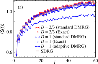
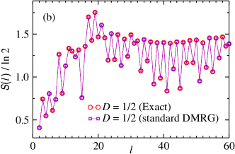
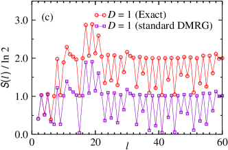
Figure 1: The EE $S$ as a function of the subsystem size $l$ for the random XX chain obtained via exact diagonalization and via the standard and adaptive DMRG methods. We have considered chains of size $L=120$ and different values of disorder strength $D$ (see legends). In panel (a) the EE is averaged over $2\,000$ disorder realizations. In panels (b) and (c), the EE is computed for a single disorder realization. The thick brown line in panel (a) corresponds to the curve $\frac{\ln 2}{6}\ln l+0.62$.

The adaptive DMRG method

We now provide the basic notion behind our adaptive DMRG method. In Fig. 1(c) we present the EE for a specific coupling configuration {$J_{1},\,J_{2},\,...,\,J_{L-1}\}$ distributed according to Eq. (2) with $D=1$. Clearly, the standard DMRG fails to reproduce the exact result for $\ell>6$. It turns out that, for this specific disorder realization, spins $7$ and $78$ are strongly entangled and locked into a singlet state to a very high degree of approximation, as predicted by the SDRG method (see Refs. Hoyos and Rigolin, 2006; Getelina et al., 2018 for a precise quantification of this statement). As a consequence of the activated dynamics (3), its effective excitation energy can be smaller than the standard DMRG error, which we have set as $\sim 10^{-10}$. In that case, the standard DMRG method could easily get stuck in an excited/metastable state and miss the $\approx\ln 2$ contribution of that singlet pair to the EE for $\ell>6$.

Is it possible to recover the missing pair? As we mentioned before, increasing the number of states does not help. Here, we suggest an alternative route which works in most cases. Lowering the disorder while maintaining roughly the same realization (as explained below), the excitation gap between spins $7$ and $78$ increases, and thus, the standard DMRG method should correctly describe the EE. This is exactly the case as verified in Fig. 1(b). There, we considered the same coupling configuration as in Fig. 1(c) but with the square root taken: $\{\sqrt{J_{1}},\,\sqrt{J_{2}},\,...,\,\sqrt{J_{L-1}}\}$, which is equivalent to having the coupling constants distributed according to Eq. (2) with $D=\frac{1}{2}$. A caveat is in order here. Notice that, for the XX spin-1/2 chain, the SDRG method predicts the same RS state for chains in Figs. 1(b) and (c). Evidently, there are stronger corrections to the RS state for smaller $D$. (Hoyos and Rigolin, 2006; Getelina et al., 2018)

Given the possibility of capturing the correct ground state for weaker disorder strength, we then propose the following adaptive DMRG strategy. We start with a weakly disordered chain (say, with disorder strength $D_{0}$) where the standard DMRG method is successful. After obtaining the quasi-exact Eigenstate $\left|\Psi_{D_{0}}\right\rangle$, we use it as the initial guess in the Lanczos or Davidson procedure for the new disorder strength $D_{0}+\delta D$ (where the new couplings are simply $J_{i}^{1+\delta D/D_{0}}$). For $\delta D\ll D_{0}$, we expect $\left|\Psi_{D_{0}}\right\rangle$ to be a very good starting point for $\left|\Psi_{D_{0}+\delta D}\right\rangle$. Here, we need to use the step-to-step wave function transformation during the sweeps as described in Ref. S. R. White, 1996. We perform a few (about $4$) sweeps in order to obtain the new quasi-exact Eigenstate $\left|\Psi_{D_{0}+\delta D}\right\rangle$. Finally, we then iterate this procedure until the desired disorder strength $D$ is reached. Since the DMRG is able to obtain the quasi-exact states for small disorder strengths, by using the above procedure the DMRG will adiabatically adapt a new basis to represent the new eigenstates. (White and Feiguin, 2004) If there is no abrupt change in the energy levels (as a function of the disorder strength), it is then expected that the above procedure will find the true (low-energy) states and will not get stuck in metastable states. As we show in the following, this is indeed the case.

Our strategy certainly may sound numerically costly. However, notice that in many cases it is desirable to study many different disorder strengths $D$. Our strategy becomes a natural one when this is the case.

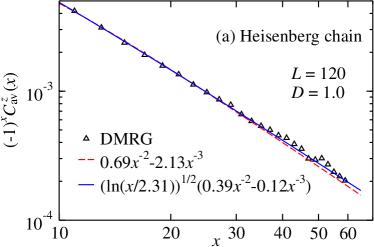
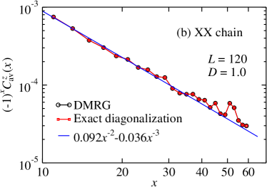
Figure 2: Log-log plot of the arithmetic average correlation function $C_{\text{av}}^{z}(x)$ vs. $x$ for (a) the Heisenberg and (b) the XX chains. The system size $L=120$, the disorder strength $D=1$ and we averaged over $1\,000$ disorder realizations. The DMRG data is obtained using the adaptive strategy. The solid and dashed lines are best fit of the DMRG data.

As a demonstration, we shown in Fig. 1(a) the arithmetic average EE obtained using our adaptive strategy starting from $D_{0}=0.4$ and increasing it in steps of $\delta D=0.06$ until we reach $D=1$. We observed that for this sequence of $D$’s the adaptive DMRG algorithm is able to reproduce the exact EE for almost all chains for $D=1$ and $L=120$. As expected, we verified that decreasing the value of $\delta D$ improves the adaptive DMRG method with the associated increase in CPU time.

Let us now discuss the spin-spin correlations (4). In order to avoid border effects, we measure $\left\langle S_{i}^{z}S_{j}^{z}\right\rangle$ in the center part of the chain by considering only $\frac{1}{4}L<i<j<\frac{3}{4}L$. The disorder average is performed over all possible distances $x=j-i$ within that range and over various different disorder realizations.

In Fig. 2 we present the adaptive DMRG results for $C_{\text{av}}(x)$ for the random spin-1/2 XX and the Heisenberg chain for systems of size $L=120$, disorder strength $D=1,$ and $10^{3}$ disorder realizations. Our results are in perfect agreement with analytical and previous numerical results in which the decay exponent is $\phi=2$ for both models. (Fisher, 1994; P. Henelius and S. M. Girvin, 1998; N. Laflorencie et al., 2004) For the Heisenberg model, it is interesting to contrast this with the clean exponent $\phi_{\text{clean}}=1$. (A. Luther and I. Peschel, 1975) Recently, a Quantum Monte Carlo study proposed a logarithmic correction to the correlation function for the Heisenberg model. Shu et al. (2016) It is not within the scope of the present work to further investigate this feature which would require longer chains and better statistics. Here, we simply report that our data are also compatible with it as shown in Fig. 1(a).

III.2 The disordered bilinear-biquadratic spin-1 chain

We now present our DMRG study on the random spin-1 chain Eq. (7). Our purpose is to use our adaptive DMRG strategy in a strongly disordered system which is not in the well-studied SU(2) infinite-randomness universality class. We then focus on the case $\theta=\frac{\pi}{4}$ which exhibits exact SU(3) symmetry [i.e., the Hamiltonian (7) becomes $H=\sum_{i}J_{i}\bm{\Lambda}_{i}\cdot\bm{\Lambda}_{i+1}+\text{const}$] placing the system in the Baryonic RS phase. (Quito et al., 2015)

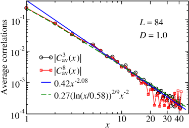
Figure 3: The arithmetic average correlation functions $C_{\text{av}}^{3}$ and $C_{\text{av}}^{8}$ [see Eq. (8)] for the SU(3)-symmetric disordered spin-1 bilinear-biquadratic chain Eq. (7) with $\theta=\frac{\pi}{4}$, system size $L=84$, and disorder strength $D=1$. The continuous blue and dashed green lines are the best fit of $C_{\text{av}}^{3}$ for $x>10$. They are compatible with the SDRG prediction $C_{\text{av}}\sim x^{-2}$. As in the spin-$1/2$ case, a logarithmic is also compatible with our data. The DMRG data are obtained using the adaptive strategy and averaging over $1\,000$ disorder realizations.

In Fig. 3, we plot the arithmetic average correlations $C_{\text{av}}^{\alpha}(x)$ Eq. (8) for $\alpha=3$ and $8$, $D=1$ and $L=84$ . The average was performed similarly to the spin-1/2 case considering all the spin pairs $S_{i}$ and $S_{j}$ in the range $\frac{1}{4}L<i<j<\frac{3}{4}L$. We verify that $C_{{\rm av}}^{\alpha}\sim x^{-\phi}$ with $\phi=2$ is consistent with our numerical data. This is a novel result which is in agreement with the predictions of the SDRG method of Sec. IV. It is interesting to compare with the clean chain exponent $\phi_{\text{clean}}=\frac{4}{3}$. (C. Itoi and M.-H. Kato, 1997) Similarly to the spin-1/2 case, the logarithmic correction of the clean system [$\propto\ln^{2/9}(x)$] (C. Itoi and M.-H. Kato, 1997) is also compatible with our data. We report that similar results were also obtained considering other system sizes $32\leq L\leq 84$ and disorder strengths $\frac{1}{4}\leq D\leq 1$. In addition, we report that (not shown) $C_{{\rm av}}^{\alpha}(x)$ oscillates with period of $3$, as a consequence of the antiferromagnetic SU(3)-symmetric character of the ground state. (Quito et al., 2015) As expected, we observed that both correlations are identical within the DMRG error.

IV Strong-disorder RG study

In this section we compute the arithmetic average correlation function $C_{\text{av}}^{\alpha}$ [see Eq. (8)] for the spin-1 chain (7) in the strong-disorder limit and in the phase of emergent Hadronic SU(3) symmetry. For that reason, we will employ the strong-disorder renormalization-group (SDRG) method developed in Refs. J. A. Hoyos and E. Miranda, 2004; Quito et al., 2015.

IV.1 The SU(3) random-singlet ground state

Figure 4: Sketch of the SU(3) random-singlet state. Sites connected by links are in a singlet state formed by $3,\,6,\,9,\,\dots$ spins. Notice the links do not overlap. Different colors represent singlets with different number of spins.

For strong disorder strength $D\gg 1$ (and very plausibly for any $D>0$), the ground state of the Hamiltonian (7) is the SU(3) random singlet state for $\frac{\pi}{4}\leq\theta<\frac{\pi}{2}$. (Quito et al., 2015) In this case, due to the emergent SU(3) symmetry, the ground-state is composed by nearly independent SU(3) singlets as sketched in Fig. 4.

Unlike the usual SU(2) spin-1/2 random-singlet state where all singlets are made of spin pairs, in the SU(3) case they can be made of any multiple of three spins. Interestingly, it has been shown that the clustering of spins disentangles from the chain energetics near the infinite-randomness fixed point. (J. A. Hoyos and E. Miranda, 2004) Therefore, the ground state depicted in Fig. 4 can be obtained in the following simple fashion: (i) one randomly chooses a neighboring spin pair in the chain and (ii) fuses them together in a new effective spin (a new spin cluster). (ii.a) If the total number of original spins in the new cluster is a multiple of three, the cluster is removed from the system since they form a singlet as in Fig. 4, otherwise, (ii.b) it remains in the system “waiting” for a new decimation. The procedure (i) and (ii) is iterated until all spins become clustered into singlets (assuming that the lattice size is a multiple of three) as in Fig. 4.

With these simplified clustering rules, it is possible to compute the probability that two original spins $\ell$ lattice sites apart become clustered in the same singlet. Assuming that they share correlations of order unity, then $C_{\text{av}}^{\alpha}$ would simply be proportional to that probability, since spins in different singlets would have exponentially small correlation. In this way, it was concluded in Ref. J. A. Hoyos and E. Miranda, 2004 that $C_{\text{av}}^{\alpha}\sim\ell^{-\frac{4}{N}}$, with $N=3$. (This generalizes to all SU($N$) random singlet states where singlets are composed by multiples of $N$ original spins).

However, as we show below, the assumption that spins belonging to the same singlet have strong correlations is not correct. Therefore, we need a better understanding of the many possible singlet states in order to correctly compute $C_{\text{av}}^{\alpha}$.

IV.2 Correlations in the SU(3) singlets

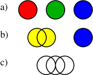
Figure 5: Schematic representation of the clustering process of three spins into a singlet state. Colors are for aesthetic purposes only.

The simplest and most common SU(3) singlet is the one made of three spins (see Fig. 5). It can be readily obtained by the anti-symmetrization of the three possible spin flavors [corresponding to Fig. 5(c)]:

$$\left|s_{\text{3-spins}}\right\rangle= \frac{1}{\sqrt{6}}\left(\left|1,0,-1\right\rangle+\left|0,-1,1\right\rangle+\left|-1,1,0\right\rangle\right.$$

$$\left.-\left|0,1,-1\right\rangle-\left|1,-1,0\right\rangle-\left|-1,0,1\right\rangle\right).$$ (9)

It is then clear that any spin pair $i,j$ in the $\left|s_{\text{3-spins}}\right\rangle$ singlet state share correlation of order unity, namely, $C_{i,j}^{\alpha}=\left\langle s_{\text{3-spins}}\left|\Lambda_{i}^{\alpha}\Lambda_{j}^{\alpha}\right|s_{\text{3-spins}}\right\rangle=-\frac{1}{3}$, for any $\alpha$.

Another way of obtaining $\left|s_{\text{3-spins}}\right\rangle$ is by following the SDRG method. (J. A. Hoyos and E. Miranda, 2004; Quito et al., 2015) One first fuses, say, spins $S_{1}$ and $S_{2}$ into a new spin-1 effective degree of freedom $\tilde{S}$ [corresponding to Fig. 5(b)], which is then decimated with spin $S_{3}$ into a singlet. With respect to the original flavors, the $\tilde{S}$ degrees of freedom are

$$\left|\tilde{1}\right\rangle =\frac{1}{\sqrt{2}}\left(\left|1,0\right\rangle-\left|0,1\right\rangle\right),$$

$$\left|\tilde{0}\right\rangle =\frac{1}{\sqrt{2}}\left(\left|1,-1\right\rangle-\left|-1,1\right\rangle\right),$$ (10)

$$\left|-\tilde{1}\right\rangle =\frac{1}{\sqrt{2}}\left(\left|0,-1\right\rangle-\left|-1,0\right\rangle\right),$$

which are obtained by projecting $\mathbf{S}_{1}+\mathbf{S}_{2}$ on the triplet manifold. The state (9) is then obtained by projecting $\tilde{\mathbf{S}}+\mathbf{S}_{3}$ on the singlet manifold $\bar{S}=0$, i.e.,

$$\left|s_{\text{3-spins}}\right\rangle=\frac{1}{\sqrt{3}}\left(\left|\tilde{1},-1\right\rangle-\left|\tilde{0},0\right\rangle+\left|-\tilde{1},1\right\rangle\right).$$ (11)

We now ask, for instance, how $C_{1,3}^{z}$ can be obtained given the knowledge of the singlet state (11). First, we notice that the correlation

$$\left\langle\tilde{S}^{z}S_{3}^{z}\right\rangle=\frac{1}{6}\left\langle\bar{S}^{2}-\tilde{S}^{2}-S_{3}^{2}\right\rangle=-\frac{2}{3}.$$ (12)

Then, we make use of the Wigner-Eckart theorem. Since $\tilde{\mathbf{S}}$ is simply $\mathbf{S}_{1}+\mathbf{S}_{2}$ projected on the triplet manifold, then $\mathbf{S}_{1}=c_{\tilde{S},S_{1},S_{2}}\tilde{\mathbf{S}}$. Since we will need to deal only with the case $S_{1}=S_{2}=\tilde{S}=1$, we lighten the notation by $c_{\tilde{S},S_{1},S_{2}}=c=\frac{1}{2}$ which can be obtained by projecting $\mathbf{S}_{1,2}$ in the multiplet (10). Finally, we have that

$$\left\langle S_{1,2}^{\alpha}S_{3}^{\beta}\right\rangle=c\left\langle\tilde{S}^{\alpha}S_{3}^{\beta}\right\rangle=-\frac{\delta_{\alpha,\beta}}{3}.$$ (13)

We now ask about the correlations between $S_{1}$ and $S_{2}$. For instance,

$$\left\langle S_{1}^{z}S_{2}^{z}\right\rangle=\frac{1}{6}\left\langle\tilde{S}^{2}-S_{1}^{2}-S_{2}^{2}\right\rangle=-\frac{1}{3}.$$ (14)

With these results, we recover that $C_{i,j}^{\alpha}=\left\langle s_{\text{3-spins}}\left|\Lambda_{i}^{\alpha}\Lambda_{j}^{\alpha}\right|s_{\text{3-spins}}\right\rangle=-\frac{1}{3}$, since it can be verified that the three-spin singlet is also an SU(3) singlet.

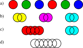
Figure 6: Schematic representation of the clustering process of six spins into a singlet state. Colors are for aesthetic purposes only.

Before generalizing these results to other singlets, let us examine the case of singlets composed by 6 spins. They can be formed in many different ways. For our purpose, let us examine only the case in which spins $S_{1}$ and $S_{2}$ are fused together in the new effective spin $\tilde{S}_{1}$. Likewise spins $S_{3}$ and $S_{4}$ ($S_{5}$ and $S_{6}$) become locked into the new effective spin $\tilde{S}_{2}$ ($\tilde{S}_{3}$) (see Fig. 6). The resulting singlet is obtained by anti-symmetrizing the effective flavors of $\tilde{S}_{1}$, $\tilde{S}_{2}$ and $\tilde{S}_{3}$, just as in the three-spin case, resulting in the singlet $\left|s_{\text{6-spins(a)}}\right\rangle$ given by (9) with the flavors $m$ replaced by $\tilde{m}$ in (10) [corresponding to Fig. 6(d)]. Less straightforwardly, we can fuse spins $\tilde{S}_{1}$ and $\tilde{S}_{2}$ into the new effective spin-1 $\tilde{\tilde{S}}$ [the flavors of which are given by (10) with $\tilde{m}\rightarrow\tilde{\tilde{m}}$ and $m\rightarrow\tilde{m}$], and then fuse $\tilde{\tilde{S}}$ with $\tilde{S}_{3}$ into the $\bar{S}=0$ singlet state $\left|s_{\text{6-spins(a)}}\right\rangle$ [corresponding to Figs. 5(c) and (d)] given by (11) with with $\tilde{m}\rightarrow\tilde{\tilde{m}}$ and $m\rightarrow\tilde{m}$ (as before).

Let us now compute the correlations. Consider for instance $C_{1,2}^{z}=\left\langle S_{1}^{z}S_{2}^{z}\right\rangle=\left\langle s_{\text{6-spins(a)}}\left|S_{1}^{z}S_{2}^{z}\right|s_{\text{6-spins(a)}}\right\rangle$. Although the singlet state is a different one, the correlation is just as in the three-spin case (14) yielding $C_{1,2}^{\alpha}=C_{3,4}^{\alpha}=C_{5,6}^{\alpha}=-\frac{1}{3}$ for any $\alpha$ (due to symmetry). Hence, as in the three-spin singlet case, there are strong correlations. Notice this strong correlation is a general feature when two original spins are decimated together into an $\tilde{S}=1$ cluster. Afterwards, renormalizations involving $\tilde{S}$ do not change the correlation between the original spins.

However, the correlations between other spin pairs are much weaker. Consider for instance $C_{1,3}^{z}$. Making use of the Wigner-Eckart theorem, then $\left\langle S_{1}^{z}S_{3}^{z}\right\rangle=c^{2}\left\langle\tilde{S}_{1}^{z}\tilde{S}_{2}^{z}\right\rangle=-\frac{1}{3}c^{2}$, since $\tilde{\mathbf{S}}_{1}$ and $\tilde{\mathbf{S}}_{2}$ are fused into a $\tilde{\tilde{S}}=1$ cluster from which follows (14). Finally, let us compute $C_{1,5}^{z}$. We will need to compute $\left\langle\tilde{\tilde{S}}^{z}\tilde{S}_{3}^{z}\right\rangle=-\frac{2}{3}$ since they fuse into a singlet, and thus follows (12). From the Wigner-Eckart theorem, $\left\langle S_{1}^{z}S_{5}^{z}\right\rangle=c^{2}\left\langle\tilde{S}_{1}^{z}\tilde{S}_{3}^{z}\right\rangle=c^{3}\left\langle\tilde{\tilde{S}}^{z}\tilde{S}_{3}^{z}\right\rangle=-2c^{3}/3$.

We then conclude that, by symmetry, $C_{i,j}^{\alpha}=-\frac{1}{12}$ for all other pairs $(i,j)$ that are not ($1,2$), ($3,4$) or ($5,6$). The important feature, as we show below, is that some longer-ranged correlations pick up powers of $c$, and thus, can be exponentially smaller in larger clusters.

We are now in a position to compute the correlations between spins $S_{i}$ and $S_{j}$ belonging to a generic SU(3) singlet. Since they belong to the same singlet cluster, they will be fused together at some point of the SDRG flow. Let $\tilde{S}$ be the effective cluster they first become fused together. Also, let $\tilde{S}_{i}$ and $\tilde{S}_{j}$ be the effective clusters that originated $\tilde{S}$. Necessarily, spin $S_{i}$ ($S_{j}$) belongs to cluster $\tilde{S}_{i}$ ($\tilde{S}_{j}$). Then $\left\langle\tilde{S}_{i}^{z}\tilde{S}_{j}^{z}\right\rangle=\frac{1}{6}\left\langle\tilde{S}^{2}-\tilde{S}_{i}^{2}-\tilde{S}_{j}^{2}\right\rangle=\frac{1}{6}\left(\tilde{S}\left(\tilde{S}+1\right)-4\right)$ and $C_{i,j}^{z}=c^{k_{i}+k_{j}}\left\langle\tilde{S}_{i}^{z}\tilde{S}_{j}^{z}\right\rangle$, where $k_{i}$ ($k_{j}$) is the number of fusions undergone by $S_{i}$ ($S_{j}$) before $\tilde{S}_{i}$ is clustered with $\tilde{S}_{j}$. Finally, by symmetry,

$$C_{i,j}^{\alpha}=\frac{1}{6}\left(\tilde{S}\left(\tilde{S}+1\right)-4\right)c^{k_{i}+k_{j}},$$ (15)

for any spins belonging to the same singlet cluster and $c=\frac{1}{2}$. Recall that $\tilde{S}=0$ ($1$) when the effective clusters of $S_{i}$ and $S_{j}$ are fused together into a singlet (triplet) state.

IV.3 Mean correlation function

Having computed the correlation between two spins belonging to the same cluster (15), we now proceed to compute the arithmetic mean correlation function (8). Following the SDRG philosophy, spins in different singlet clusters share very weak correlations and therefore, do not contribute to the long-distance behavior of $C_{\text{av}}^{\alpha}$ (we set $C_{i,j}^{\alpha}=0$ for $i$ and $j$ belonging to different spin singlet clusters).

We then proceed by numerically implementing the SDRG method as explained in the following. We focus on the SU(3)-symmetric spin chain $\theta=\frac{\pi}{4}$ in the Hamiltonian (7) (but this also applies to $\frac{\pi}{4}\leq\theta<\frac{\pi}{2}$) with coupling constants drawn from the distribution (2). We then decimate the entire chain using the SDRG rules as explained in Refs. J. A. Hoyos and E. Miranda, 2004; Quito et al., 2015. We choose the largest coupling in the system, say, $J_{2}$, and decimate the corresponding effective cluster spin pair either by (i) removing them from the system (which happens when the total number of original spins in both clusters is a multiple of three) or (ii) by clustering them in a new effective spin-1 cluster (which happens otherwise). In the case (i) of a singlet decimation, the neighboring spin clusters become connected via a weaker coupling of magnitude $\tilde{J}=\frac{2J_{1}J_{3}}{9J_{2}}$. On the other hand for the case (ii), the new couplings connecting to the new effective spin cluster are $\tilde{J}_{1,3}=\frac{1}{2}J_{1,3}$.

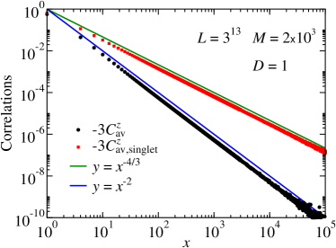
Figure 7: The arithmetic mean spin-spin correlation $C_{\text{av}}^{\alpha}$ function as a function of the spin separation $x$ computed for distances $x=1+3n$, with $n\in\mathbb{N}_{+}$. For comparison, we also show the singlet spin-spin correlation $C_{\text{av,singlet}}^{\alpha}$ (see text). The system size is $L=3^{12}$ (where periodic boundary conditions were considered), the disorder parameter is $D=1$, and we have averaged over $M=2\times 10^{3}$ different disorder realizations.

After the entire chain is decimated, the SDRG ground state is obtained (see Fig. 4) and the correlations can be computed via (15). Averaging over all distances and over $M$ different disorder realizations, $C_{\text{av}}^{\alpha}$ is obtained as shown in Fig. 7. For comparison, we also plot the arithmetic mean singlet-correlation $C_{\text{av,cluster}}^{\alpha}$, which is simply the probability of finding two spins belonging to the same spin singlet cluster multiplied by $-\frac{1}{3}$. Notice that $C_{\text{av,cluster}}^{\alpha}(x)\sim x^{-\phi_{\text{cluster}}}$ with $\phi_{\text{cluster}}=\frac{4}{3}$ (as shown in Ref. J. A. Hoyos and E. Miranda, 2004) and that $C_{\text{av}}^{\alpha}(x)\sim x^{-\phi}$ with $\phi=2$. We have studied chains of different sizes and different disorder strengths and verified the universality of these exponents.

It is desirable to obtain an analytical derivation for the universal exponents $\phi=2$ and $\phi_{\text{cluster}}=\frac{4}{3}$. We will learn from this quest that $C_{\text{av,{\rm cluster}}}$ is dominated by spin pairs in large clusters composed by several original spins, and that the exponential suppression of correlations after many clusterings [see Eq. (15)] is so strong that $C_{\text{av}}$ becomes dominated by original spins pairs that become locked together in a cluster for the first time.

We start our analysis with $Q(t;\rho)$: the probability of finding a spin cluster composed of $t$ original spins at the length scale $x=\rho^{-1}=L/N_{T}$ where $N_{T}$ is the total number of spin clusters at that length scale, $\rho$ is simply the density of spin clusters in the lattice, and $L$ is the original number of lattice sites. As mentioned in Sec. IV.1, the SDRG clustering rules disentangle from the system energetics in the later stages of the SDRG flow. In that case, the flow equation for $Q$ becomes much simpler:

$$\text{d}[L\rho Q]=\text{d}N_{\text{dec}}\left(-2Q(t;\rho)+Q\stackrel{{\scriptstyle t}}{{\hexstar}}Q\right).$$ (16)

The left-hand-side of Eq. (16) is simply the change on the number of clusters containing $t$ original spins when the system density changes from $\rho$ to $\rho+\text{d}\rho$. $\text{d}N_{\text{dec}}$ is the corresponding total number of decimations which is related to $\rho$ via $\text{d}[L\rho]=-\left(2p+q\right)\text{d}N_{\text{dec}}$, with $p$ ($q=1-p$) being the probability of a (non-) singlet decimation and $\text{d}[L\rho]$ being the corresponding change in the total number of clusters. For the SU(3) case, $p=q=\frac{1}{2}$. Generically for the SU($N$) case, $p=\frac{1}{N-1}$. Recall that for each singlet-like decimation, two clusters are removed while for a non-singlet decimation, two clusters are removed but a new one is inserted. The first term on the right-hand-side of Eq. (16) accounts for the removal of the two decimated clusters in every decimation. The last term accounts for the insertion of the new cluster containing the total number of spins: $Q\stackrel{{\scriptstyle t}}{{\hexstar}}Q=\sum_{t_{1},t_{2}}Q(t_{1})Q(t_{2})\delta_{t,t_{1}+t_{2}}(1-\delta_{t,N}-\delta_{t,2N}-\dots)$. The term inside the parentheses ensures that only non-singlet decimations contribute. In order to keep the analysis simple, from now on we will allow $Q(t)$ to be non-zero also for $t$ a multiple of $N$ and recast this term as $qQ\stackrel{{\scriptstyle t}}{{\otimes}}Q=q\sum_{t_{1},t_{2}}Q(t_{1})Q(t_{2})\delta_{t,t_{1}+t_{2}}$. Exchanging $Q\stackrel{{\scriptstyle t}}{{\hexstar}}Q$ by $qQ\stackrel{{\scriptstyle t}}{{\otimes}}Q$ is equivalent to replacing the precise occurrence of a non-singlet decimation by its average occurrence. Therefore, this simplification cannot change the large-$t$ behavior of $Q(t;\rho)$, and thus, we expect to obtain the correct value of the universal exponents $\phi$ and $\phi_{\text{cluster}}$.

We now try a solution of type $Q(t;\rho)=A_{\rho}e^{-B_{\rho}(t-1)}$, where $A_{\rho}$ and $B_{\rho}$ are $t$-independent functions. From the normalization condition $\sum_{t=1}^{\infty}Q(t;\rho)=1$, our Ansatz simplifies to $Q=A_{\rho}\left(1-A_{\rho}\right)^{t-1}$. Plugging this result into the simplified flow equation, we find that

$$Q\left(t;\rho\right)=\rho^{\gamma}\left(1-\rho^{\gamma}\right)^{t-1},$$ (17)

where $\gamma=1-\frac{2}{N}$ and we have used the initial condition $Q(t;1)=\delta_{t,1}$. For comparison, we plot in Fig. 8 the probability $Q(t;\rho)$ for various different values of density $\rho$ obtained via the numerical implementation of the SDRG procedure as explained for Fig. 7. As expected, the large-$t$ behavior is well described by our simplified result (17), although we cannot rule out a power-law correction to the exponential dependence on $t$.

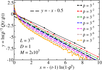
Figure 8: The probability $Q(t;\rho)$ of finding a spin cluster composed of $t$ original spins at the density scale $\rho$ for various different density values. The data were obtained via the numerical implementation of the SDRG procedure where the parameters used are the same as in Fig. 7. The dashed line is the simplified prediction Eq. (17) with an offset for better comparison. The lines are guide to the eyes.

We are now able to obtain the leading behavior of $C_{\text{av,cluster}}^{\alpha}$. This is proportional to the probability that any two original spins, $x$ lattice sites apart, are in neighboring spin clusters at the density scale $\rho=x^{-1}$. (We can associate $x$ with $\rho^{-1}$ because the size of the clusters is of order of the mean distance between them.) Thus, we need the probability $R_{T}(\rho)$ that a certain original spin is still active (i.e., belonging to some spin cluster) at the density scale $\rho$. This is proportional to the total number of original spins in the effective chains. Thus, $R_{T}\propto\rho\sum_{t}tQ\left(t;\rho\right)=\rho\bar{t}=\rho^{1-\gamma}$ and

$$C_{\text{av,cluster}}^{\alpha}\sim\left(R_{T}(\rho)\right)^{2}\propto x^{-\phi_{\text{cluster}}},$$ (18)

with $\phi_{\text{cluster}}=\frac{4}{N}$, which recovers the result of Ref. J. A. Hoyos and E. Miranda, 2004.

In order to compute $C_{\text{av}}^{\alpha}$, we need the probability $R(t;\rho)=R_{T}\left(\rho\right)Q\left(t;\rho\right)$ of finding an original spin in a cluster composed by $t$ original spins at the density scale $\rho$. The correlations in Eq. (15) are incorporated in the following approximate way. We assume that contribution to the correlations coming from spins $S_{i}$ and $S_{i+x}$ is $\propto c^{2k}$ where $k$ is the largest integer smaller then $\frac{t_{i}+t_{i+x}}{N}$, where $t_{i}$ and $t_{i+x}$ are respectively the number of original spins on the clusters containing $S_{i}$ and $S_{i+x}$ when they are fused together at the density scale $\rho=x^{-1}$. Thus, Eq. (18) is generalized to

$$C_{\text{av}}^{\alpha} \sim\sum_{k=0}^{\infty}c^{2k}\sum_{kN<t_{i}+t_{j}\leq(k+1)N}R(t_{i};\rho)R(t_{j};\rho)$$ (19)

$$=\rho^{2}\left(1+\sum_{n=1}^{\infty}a_{n}\left(1-\rho^{\gamma}\right)^{n}\right)\sim ax^{-\phi},$$ (20)

where the second sum in (19) denotes a double sum over all values $t_{i}$ and $t_{j}$ obeying the constraint $kN<t_{i}+t_{j}\leq(k+1)N$. In the last passage, we considered only the long-distance regime $x\gg 1$ where we found a universal exponent $\phi=2$ and the constant

$$a=\sum_{k=0}^{\infty}\frac{c^{2k}\left((2k-1)N^{2}-N\right)}{2}=\frac{\left(N+N^{2}\right)c^{2}+N^{2}-N}{2\left(1-c^{2}\right)^{2}}.$$ (21)

We therefore recover the numerical SDRG results in Fig. 7 and provide a simple theory for the DMRG results of Sec. III. It is interesting to track the contributions to the constant (21). The exponential decay of correlations upon many projections (15) dictates that the main contribution comes from those spins in smaller clusters. For this reason, the result (20) is applicable to any SU($N$) random singlet state.

V Conclusions

We have devised an adaptive density-matrix renormalization-group (DMRG) method able to tackle strongly disordered random systems and applied it to the random antiferromagnetic spin-1/2 chain and to the random spin-1 with bilinear and biquadratic interactions.

The adaptive DMRG method was able to recover the known results for the spin-1/2 chain in the literature and overcome the deficiency of the standard DMRG method in capturing the entanglement between distant spins in the system. For the spin-1 chain at the SU(3) symmetric point [$\theta=\frac{\pi}{4}$ in (7)], we found that the average correlations decay as a power law with the same universal exponent as in the spin-1/2 chains, $\phi=2$. In order to confirm this result, we then developed a strong-disorder renormalization-group (SDRG) framework for computing the spin-spin correlation for all SU($N$) symmetric random-singlet states and concluded that the correlation exponent is universal and equal to $\phi=2$ for all $N\geq 2$. This result also applies to all SO($N$)-symmetric random spin chains exhibiting enlarged SU($N$) symmetry random-singlet ground states. (Quito et al., 2017a, b)

Our adaptive DMRG algorithm requires few changes with respect to the standard DMRG method and thus, can be easily implemented. The input state of our method in the high-disorder regime is self-generated and does not rely on other methods such as those of the tensor-network-based algorithms. Finally, the convergence of our method for larger degrees of disorder can be controlled by setting smaller disorder increments. Therefore, our method may be suitable to study other quantum phase transitions driven by the disorder strength such as many-body localization transitions.