3D Simulations of Planet Trapping at Disc-Cavity Boundaries

Abstract

Inward migration of low-mass planets and embryos of giant planets can be stopped at the disc-cavity boundaries due to co-orbital corotation torque. We performed the first global three-dimensional (3D) simulations of planet migration at the disc-cavity boundary, and have shown that the boundary is a robust trap for low-mass planets and embryos. A protoplanetary disc may have several such trapping regions at various distances from the star, such as at the edge of the stellar magnetosphere, the inner edge of the dead zone, the dust-sublimation radius and the snow lines. Corotation traps located at different distances from a star, and moving outward during the disc dispersal phase, may possibly explain the observed homogeneous distribution of low-mass planets with distance from their host stars.

1 Introduction

Thousands of planets were discovered by COROT, Kepler, K2, and other space and ground-based telescopes (3,989 planets, February 19 2019, see exoplanet.eu; see also, e.g. Borucki et al. 2010). The current distribution of planets reflects the complex history of their formation in protoplanetary discs, and their dynamical interaction with their discs, host stars, and other planets (e.g. Winn & Fabrycky 2015).

Most of the planets observed at the distances of 0.1-1 AU from their host stars have relatively low masses, $M_{p}\sim 1-30M_{\oplus}$. These planets are almost homogeneously distributed with respect to their orbital periods (e.g. Fressin et al. 2013; Winn & Fabrycky 2015). These planets have different radii in the range of $1R_{\oplus}\lesssim R_{p}\lesssim 4R_{\oplus}$ (see Fig. 1 from review by Kaltenegger 2017; see also Zeng, Sasselov & Jacobsen 2016). Some of them have higher densities and are expected to be predominantly rocky, while others have lower densities and are expected to be predominantly gaseous. Gaseous planets are expected to form when a significant amount of gas is present in the disc during planet formation. If a disc is present during planet formation, then the newly-formed planets interact with the disc gravitationally and migrate. Their migration time scale is expected to be lower than the time scale of planet formation (e.g. Lin & Papaloizou 1986).

In addition, a significant number of more massive, Jupiter-sized planets are present in the planetary data set. These planets are expected to form in gaseous discs, starting from seed rocky cores (embryos) of a few Earth masses (e.g. Pollack et al. 1996). These rocky cores can also migrate rapidly and fall onto the star before a planet can form.

Low-mass planets and rocky embryos of giant planets are expected to migrate in the Type I regime, where the planet does not open a gap. The torque acting on a planet consists of two components: the differential Lindblad torque and the corotation torque (Goldreich & Tremaine, 1979, 1980; Lin & Papaloizou, 1979; Ward, 1986, 1997). The Lindblad torque arises from the tidal interaction of a planet with the disc, which leads to the formation of two spiral density waves that exert positive and negative torques on the planet. The cumulative Lindblad torque is typically negative. The corotation torque arises from the interaction of a planet with the co-orbital matter; it is usually positive. In a typical accretion disc, where the surface density smoothly decreases with distance from the star (e.g. Hayashi 1981), the negative Lindblad torque is usually larger (in absolute value) than the corotation torque, and the planet migrates inward towards the star. For a planet located at a few AU, the time scale of migration is smaller than both the time scale of planet formation and the life time of the disc. Therefore, many planets and rocky embryos are expected to migrate to small radii, and may fall onto their host stars (e.g. Lin & Papaloizou 1986, see also review paper by Kley & Nelson 2012). This picture of migration does not correspond to the observed dispersed distribution of low-mass planets with distance from their host stars (e.g. Winn & Fabrycky 2015).

In recent years, different factors that may slow down or reverse migration were taken into account, such as (a) density and temperature gradients in the disc (e.g. Masset 2001; DÁngelo & Lubow 2010; Lega et al. 2014; Masset & Benitéz-Llambay 2016), (b) turbulence in the disc (e.g. Nelson 2005), (c) magnetic fields (e.g. Terquem 2003; Fromang et al. 2005; Baruteau et al. 2011; Comins et al. 2016; McNally et al. 2017; McNally et al. 2018), and other factors (see review papers by Masset 2008; Kley & Nelson 2012; Baruteau et al. 2014, 2016).

In particular, it has been shown that, if some parts of the disc have positive density gradients, then the positive corotation torque dominates over the negative Lindblad torque, and the planets can either migrate outward or the migration may stall (e.g. Masset 2001; Tanaka et al. 2002; Masset et al. 2006a; Masset 2008; Paardekooper & Papaloizou 2009a).

Strong positive density gradients are expected at the transition region between the disc and the inner gap or cavity, where the density is lower than that in the disc (Masset et al., 2006a). Such cavities can be associated with transition regions in the disc, such as the magnetospheric boundary, a dead zone, the dust sublimation radius, and the radius of the snow line (e.g. Masset et al. 2006a; Morbidelli et al. 2008; Ida & Lin 2008; Hasegawa & Pudritz 2011).

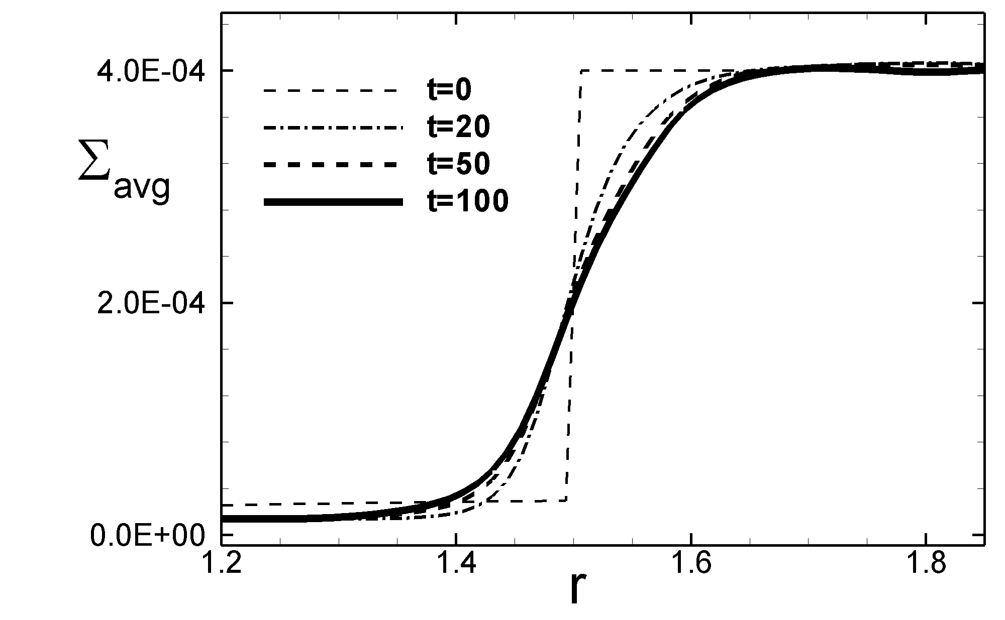
Figure 1: Left panels: $rz$-slices through the disc showing the density distribution (colour background) at $t=0,20,100$. Vertical line in the top panel shows the position of the sharp density gradient at $t=0$. Dashed lines in the middle and bottom panels show approximate boundaries for the large positive gradient ($1.4\lesssim r\lesssim 1.6$) at $t=20$ and $t=100$. Right panel: radial distribution of the azimuthally-averaged surface density, $\Sigma_{\rm avg}$, at the disc-cavity boundary at $t=0,20,50,100$.

Masset et al. (2006a) studied the effects of corotation torque on the migration of planets in the vicinity of a cavity edge using 2D hydrodynamic simulations. In their study, low-mass planets (1.3-15 $M_{\oplus}$) were allowed to migrate in an accretion disc with a lower-density cavity. Far from the cavity boundary, planets migrated inward as usual due to the differential Lindblad torque. However, as the planets approached the density transition, the authors found that the corotation torque contributed a positive torque, creating a stable planet trap where the net torque is zero and the inward migration is halted. Instead of migrating into the cavity (as would be expected if the Lindblad resonance were dominant), the migration of planets halts while they are still in the disc due to the action of the corotation torque. The authors have shown that planets are stably trapped at the boundary, and when the boundary changes its position the trapped planets move together with the boundary.

Morbidelli et al. (2008) investigated the planet trap mechanism as a way of avoiding the inspiral problem, focusing on the case where the planet embryos are trapped at the cavity boundary, allowing for a gradual buildup of giant-planet cores.

Liu et al. (2017) studied the trapping of low-mass planets at a sharp disc-magnetosphere boundary using a semi-analytical approach. Here, the authors have shown that the one-sided positive corotation torque at the boundary is larger than the one-sided negative Lindblad torque for a wide range of low-mass planets. The authors considered evolving discs, where the disc-magnetosphere boundary moves outward during the disc dispersal phase. They suggested that the planets move with the boundary as long as the surface density in the disc is sufficiently high. The authors proposed this mechanism for explaining the observed dispersed distribution of planets at $r\lesssim 1$ AU .

In this study, we investigate for the first time the migration of low-mass planets and embryos at the disc-cavity boundary using global three-dimensional (3D) simulations. In Sec. 2, we discuss the problem setup. In Sec. 3, we show the details of our numerical model. In Sec. 4, we describe our results. In Sec. 5, we discuss the applications of our model. In Sec. 6, we conclude. In Appendixes A and B, we show the results of our simulations for discs with different aspect ratios and at different viscosities in the disc, respectively.

2 Problem setup

We consider the migration of the low-mass planets at the disc-cavity boundary using global 3D simulations.

Initial conditions.

The simulation region consists of a disc, which is truncated at the radius of $r=r_{d}=r_{\rm cav}$, a low-density cavity located at $r<r_{\rm cav}$, and a low-density corona above and below the disc. Initially, the matter in the disc is dense and cold, while the cavity and corona are filled with hot, lower density gas. In most of the simulation runs, we take a disc with an aspect ratio of $h=H/r=0.03$, which is determined at time $t=0$ at the inner edge of the disc, $r=r_{\rm cav}$. The scale height of the disc is $H=(c_{s}/v_{\rm K})r$, where $c_{s}$ and $v_{K}$ are the sound speed and Keplerian velocity, respectively .

We calculate the equilibrium distribution of density and pressure in the disc and corona using the following method. First, we determine the equilibrium in the equatorial plane. The initial radial density and pressure distributions are given by

$$\rho(r,0)=\left\{\begin{array}[]{lr}\rho_{\rm cav}\left(\frac{r}{r_{\rm cav}}\right)^{-n}&{\rm if}\ r<r_{\rm cav}\\ \rho_{\rm d}\left(\frac{r}{r_{\rm cav}}\right)^{-n}&{\rm if}\ r\geq r_{\rm cav}\end{array}\right.\quad,$$ (1)

and

$$p(r,0)=p_{\rm d}\left(\frac{r}{r_{\rm cav}}\right)^{-l}\quad.$$ (2)

Here, $\rho_{\rm cav}$, $\rho_{\rm d}$ and $p_{\rm d}$ set the cavity density, disc density and pressure, respectively, at $r=r_{\rm cav}$ (in the equatorial plane). Parameters $n$ and $l$ specify the radial profile of the disc density and pressure, respectively. We use the values $n=1.5$ and $l=1.5$ in all simulation runs.

Near the inner edge of the disc ($r=r_{d}$), the pressure in the inner disc should be equal to the pressure in the cavity, $p_{\rm d}=p_{\rm cav}$. In the equatorial plane, the dimensionless temperature is related to density and pressure by the ideal gas law, ${\cal R}T(r,0)=p(r,0)/\rho(r,0)$ .

Next, we assume that there is a hydrostatic equilibrium in the vertical direction and build the 3D distribution of density and pressure:

$$\rho(r,z)=\rho(r,0)\exp\left(\frac{\Phi(r,0)-\Phi(r,z)}{{\cal R}T(r,0)}\right)~{},$$ (3)

where $\Phi(r,z)=-GM_{*}/(r^{2}+z^{2})^{1/2}$ is the gravitational potential of the star. The expression for pressure is analogous. The azimuthal velocity $v_{\phi}$ is set by the balance of gravity and pressure gradient forces in the radial direction:

$$v_{\phi}(r,z)=\sqrt{r\left(\frac{\partial\Phi}{\partial r}+\frac{1}{\rho}\frac{\partial p}{\partial r}\right)}~{}.$$ (4)

These formulae allow us to start from a quasi-equilibrium configuration for the disc and the cavity.

We calculate the surface density distribution in the disc by integrating the volume density $\rho$ in the $z-$direction:

$$\Sigma=\int{\rho dz}\propto H\rho\propto\frac{c_{s}\rho}{\Omega}\propto\frac{\sqrt{p\rho}}{\Omega}\propto r^{\frac{3-n-l}{2}}.$$ (5)

Here, $c_{s}\propto\sqrt{p/\rho}$ is the sound speed. The slopes of $n=1.5$ and $l=1.5$ in the equatorial density and pressure distributions result in a flat surface density profile, $\Sigma=const$ the disc. Note that the corotation torque strongly depends on the local positive density gradient at the disc-cavity boundary, while the density distribution at larger (and smaller) distances from the cavity is not as important. This is why we choose this initial density distribution and fixed it in all simulation runs.

Dimensionalization.

The simulations are dimensionless and can be applied to cavities located at different distances from the star. For dimensionalization, we choose a reference scale, $r_{0}$, and place the cavity at the radius of $r_{\rm cav}=1.5r_{0}$. The reference mass is set to the mass of the star, $M_{0}=M_{*}$. The reference velocity is given by $v_{0}=\sqrt{GM_{*}/r_{0}}$, corresponding to the Keplerian orbital velocity at $r=r_{0}$. We measure time in Keplerian periods of rotation at $r=r_{0}$: $P_{0}=2\pi r_{0}/v_{0}$. The reference density is $\rho_{0}=M_{0}/r_{0}^{3}$ and the reference surface density is $\Sigma_{0}=M_{0}/r_{0}^{2}$. The reference pressure is $p_{0}=\rho_{0}v_{0}^{2}$ and the reference temperature is $T_{0}=p_{0}/(\mathcal{R}\rho_{0})$, where $\mathcal{R}$ is the specific gas constant.

The mass of the planet is given by $M_{p}=q_{p}M_{0}$. In this paper, we study the migration of planets with masses $M_{p}=5{\rm M}_{\oplus}$ and $M_{p}=15{\rm M}_{\oplus}$, which correspond to dimensionless masses $q_{p}=1.5\times 10^{-5}$ and $q_{p}=4.5\times 10^{-5}$, respectively.

For each dimensionless quantity $\widetilde{Q}$, we recover the physical value $Q$ by multiplying $\widetilde{Q}$ by the corresponding reference value, $Q_{0}$: $Q=\widetilde{Q}Q_{0}$. For example, in a disc around a 1 ${\rm M}_{\astrosun}$ star with a low-density cavity extending out to $r_{\rm cav}=1$ AU, the reference mass is $M_{0}=1{\rm M}_{\astrosun}$, the reference length is $r_{0}=0.66$ AU, the reference velocity is $36.5$ km s^-1, the reference period is $P_{0}=199$ d, and the reference surface density is $\Sigma_{0}=2\times 10^{7}$ g cm^-2. To obtain the physical values of these quantities, their reference values must then be scaled by the dimensionless values obtained from the simulations.

Our dimensionless simulations are applicable to cavities located at different distances from the star. Tab. 1 shows our reference values and the initial values used in our model. We give examples of reference values for cavities located at $r_{\rm cav}=0.1$ AU, $0.5$ AU and $1.0$ AU from the star. Corresponding reference values for distance are $r_{0}=r_{\rm cav}/1.5\approx 0.67,0.33$ and $0.067$ AU, respectively.

Initial values in the model.

The characteristic mass of the disc is $M_{\rm d0}=q_{d}M_{0}$, where $q_{d}=4\times 10^{-4}$. Initial value of the surface density in the simulations is $\Sigma_{d}(t=0)=q_{d}\Sigma_{0}$, and therefore the initial dimensionless value of the surface density is $\widetilde{\Sigma}_{d}=q_{d}=4\times 10^{-4}$. The initial dimensionless values of the surface density in the disc and in the cavity are: $\widetilde{\Sigma}_{\rm d}=4\times 10^{-4}$ and $\widetilde{\Sigma}_{\rm cav}\approx 0.072\widetilde{\Sigma}_{\rm d}$.

The initial dimensionless values of the volume density in the disc and cavity at the reference point ($r=r_{\rm cav}$) are taken to be: $\widetilde{}\rho_{\rm d}=3.35\times 10^{-3}$ and $\widetilde{}\rho_{\rm cav}=10^{-2}\widetilde{\rho}_{\rm d}=3.35\times 10^{-5}$ . Initial pressure is $\widetilde{}p_{\rm d}=2.6\times 10^{-6}$.

One can obtain dimensional values, using reference values from Tab. 1 and by multiplying dimensionless values by reference values $\rho_{0}$ and $p_{0}$. For example, for cavity, located at $r_{\rm cav}=1$ AU, we have $\rho_{0}=2\times 10^{-6}$ g cm^-3 and obtain dimensional values $\rho_{\rm d}=6.7\times 10^{-9}$ g cm^-3 and $\rho_{\rm cav}=6.7\times 10^{-11}$ g cm^-3.

Taking into account the reference surface density $\Sigma_{0}=2\times 10^{7}$ g cm^-2 (at $r_{0}=0.67$ AU), one obtains dimensional values $\Sigma_{\rm d}=8\times 10^{3}$ g cm^-2 and $\Sigma_{\rm cav}=5.6\times 10^{2}$ g cm^-2. The bottom three rows of Tab. 1 show the initial values of the disc mass, density and surface density in the disc for cavities located at different distances from the star. The right column shows different values obtained for the Minimum-Mass Solar Nebula (MMSN) at the distance of $0.67$ AU. As an example, we used the Hayashi (1981) MMSN, where the surface density distribution $\Sigma\approx 1700(r/1\rm{AU})^{-3/2}$ g cm^-2.

In this study, all of the values are given in terms of dimensionless units, except where explicitly assigned physical units. Subsequently in the text, we do not place tilde’s above dimensionless values.

Reference Unit		Reference Values			MMSN
Reference mass of the star	$M_{0}$ [${\rm M}_{\astrosun}$]	1	1	1	1
Position of the disc-cavity boundary	$r_{\rm cav}$ [AU]	0.1	0.5	1	1
Reference distance $r_{0}=r_{\rm cav}/1.5$	$r_{0}$ [AU]	0.067	0.33	0.67	0.67
Reference velocity	$v_{0}$ [km s-1]	115	51.6	36.5	36.5
Reference period	$P_{0}$ [days]	6.29	70.3	199	199
Reference density	$\rho_{0}$ [g cm-3]	$2.0\times 10^{-3}$	$1.6\times 10^{-5}$	$2.0\times 10^{-6}$
Reference surface density	$\Sigma_{0}$ [g cm-2]	$2.0\times 10^{9}$	$8.0\times 10^{7}$	$2.0\times 10^{7}$
Reference pressure	$p_{0}$ [g cm-1 s-2]	$2.6\times 10^{11}$	$4.3\times 10^{8}$	$2.7\times 10^{7}$
			Initial values in the model		MMSN
Reference mass of the disc $M_{\rm d0}=4\times 10^{-4}M_{0}$	$M_{\rm d0}$ [${\rm M}_{\astrosun}$]	$4.0\times 10^{-4}$	$4.0\times 10^{-4}$	$4.0\times 10^{-4}$
Initial density in the disc at $r=r_{\rm cav}$	$\rho_{d}$ [g cm-3]	$8.0\times 10^{-7}$	$6.4\times 10^{-9}$	$8.0\times 10^{-10}$
Initial surface density in the disc	$\Sigma_{d}$ [g cm-2]	$8.0\times 10^{5}$	$3.2\times 10^{4}$	$8.0\times 10^{3}$	$1.7\times 10^{3}$

Table 1: Top rows: reference values calculated for different positions of the disc-cavity boundary $r_{\rm cav}$. Bottom rows: the reference mass of the disc, $M_{d0}$ and initial values of density and surface density taken in the model. The last column shows the typical values from the model of the MMSN at the distance of $1$ AU (Hayashi, 1981).

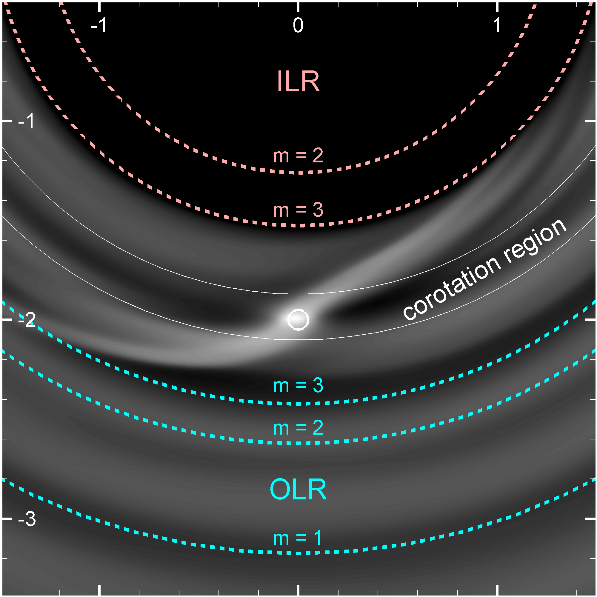
Figure 2: A schematic diagram of various resonance locations for a planet of mass $M_{p}=15M_{\oplus}$. The plot shows the corotation region (plotted here as $r_{p}\pm 3r_{\rm Hill}$) and the locations of the $m=1-3$ Lindblad resonances.

3 Numerical model

Our code has a hydrodynamics module that models the gas dynamics in the disc, as well as a planet module that computes the orbital trajectory of the planet that migrates due to interaction with the disc. In our model, the planet and disc only interact gravitationally. The disc is assumed to have negligible self-gravity. We investigate this problem in global 3D cylindrical $\mathbf{r}=(r,\phi,z)$ coordinates, implemented in a Godunov-type code that was developed by our group (Koldoba et al., 2016).

The equations of hydrodynamics.

We model the evolution of the accretion disc using 3D equations of hydrodynamics, which can be compactly written as

$$\partial_{t}\boldsymbol{U}+\nabla\cdot\boldsymbol{F}(\boldsymbol{U})=\boldsymbol{Q}~{},$$ (6)

where $\boldsymbol{U}$ is the vector of conserved variables and $\boldsymbol{F}(\boldsymbol{U})$ is the vector of fluxes:

$$\boldsymbol{U}=\left[\rho,\rho S,\rho\boldsymbol{v}\right]^{T},\quad\boldsymbol{F}(\boldsymbol{U})=\left[\rho\boldsymbol{v},\rho\boldsymbol{v}S,\mathbfsf{M}\right]^{T},$$ (7)

and $\boldsymbol{Q}=[0,0,-\rho\nabla\Phi]$ is the vector of source terms. In the above equations, $\rho$ is the fluid density, $S\equiv p/\rho^{\gamma}$ is the function of the specific entropy (entropy per unit mass, which we will simply call entropy in this paper) with $\gamma=5/3$, $\boldsymbol{v}$ is the velocity vector, $\Phi$ is the gravitational potential of the star-planet system (given later on in this section) and $\mathbfsf{M}$ is the momentum tensor, with components $M_{ij}=\rho v_{i}v_{j}+\delta_{ij}p~{},$ where $\delta_{ij}$ is the Kronecker delta function and $p$ is the fluid pressure. In our code, we use the entropy balance equation instead of the full energy equation, because in problems which we solve, the shock waves are not expected, at least shock waves of large intensity where we cannot neglect the energy dissipation. The advantage of this approach is that in the entropy balance equation (compared with the full energy equation) there are no terms which significantly differ in their values .

We include a viscosity term, with the viscosity coefficient in the form of $\alpha-$viscosity, $\nu_{\rm vis}=\alpha c_{s}H$. In most of our simulations we take $\alpha=0$, so that the disc does not change its shape during the simulation runs .

Migration of a planet.

To calculate the migration of a planet, we first calculate the gravitational potential of the star-planet system, which is given by

$$\Phi=-\frac{GM_{*}}{|\mathbf{x}|}-\frac{GM_{p}}{(|\mathbf{x}-\mathbf{x}_{p}|^{2}+\epsilon^{2})^{1/2}}+\frac{GM_{p}}{|\mathbf{x}_{p}|^{3}}\mathbf{x}\cdot\mathbf{x}_{p},$$ (8)

where $\epsilon$ is a smoothing radius that is added to prevent divergence at the planet’s location (e.g. Nelson et al. 2000). In 3D simulations there are no specific physical restrictions to this value (compared with the 2D simulations, e.g. Müller et al. 2012), so that any small value can be taken at which the numerical solution near the planet is stable. However, the smallest possible value is desirable, because a large smoothing radius may decrease the value of the corotation torques acting on the planet (e.g. Masset 2002). In our models, we took a value equal to two grid cells at $r=1.5$: $\epsilon=2\Delta r\approx 0.025$. Test simulations at smaller and larger values of $\epsilon$ have shown that the solution is stable at this value of the smoothing parameter. The total mass of the disc is small compared to the mass of the star, and hence we neglect the contribution to the potential from the disc matter.

Next, we calculate the force per unit mass acting on the disc, $\mathbf{f}=-\nabla\Phi$, or:

$$\mathbf{f}=-\frac{GM_{*}}{|\mathbf{x}|^{3}}\mathbf{x}-\frac{GM_{p}}{(|\mathbf{x}-\mathbf{x_{p}}|^{2}+\epsilon^{2})^{3/2}}\mathbf{(x-x_{p})}-\frac{GM_{p}}{|\mathbf{x}_{p}|^{3}}\mathbf{x_{p}}~{}.$$ (9)

The first and second terms represent the gravitational forces from the star and the planet, respectively. The final term accounts for the fact that the coordinate system is centered on the star, which is a non-inertial frame due to the presence of the companion planet.

Numerical method.

To solve the hydrodynamic equations, we use the Godunov-type code developed in our group for solving different hydro- and magnetohydrodynamic problems in astrophysics and for modelling migration of planets in accretion discs (Koldoba et al., 2016). In this paper, we use the hydrodynamic, three-dimensional version of the code.

Our code is similar in many respects to other codes which use Godunov-type method, such as PLUTO (Mignone et al., 2007), FLASH (Fryxell et al., 2000) and ATHENA (Stone et al., 2008). We solve the entropy conservation equations in place of the full energy equation.

To calculate the migration of a planet, we use earlier developed approaches (e.g. Kley 1998; Masset 2000). Namely, we calculate the potential and forces acting from the planet onto the disc and calculate the position of a planet using the value of this force with an opposite sign (see also Kley & Nelson 2012).

We rotate our numerical grid with a planet and the position of the planet (relative to the grid) is fixed. Such approach has been suggested by Kley (1998) and has been used in a number of planetary codes. In this approach, matter flow near the planet can be calculated with a higher accuracy compared to cases of non-rotating grids. In many recent codes, an orbital advection scheme (the FARGO algorithm), is used, where the layers of the numerical grid have differential rotation (see Masset 2000 and Bentez-Llambay & Masset 2016 for 2D and 3D versions of the FARGO code) .

The equations of hydrodynamics are integrated numerically using an explicit conservative Godunov-type numerical scheme (Koldoba et al., 2016). In our numerical code the dynamical variables are determined in the “centers” of cells. For calculation of fluxes between the cells we use the HLLD Riemann’s solver developed by Miyoshi & Kusano (2005) and modified for using the equation for the entropy balance (see also Miyoshi et al. 2010) and grid rotation. For better spatial resolution, we performed reconstruction of the primitive variables to the boundaries between calculated cells with the help of second-order limiter. Integration of the equations with time is performed with a two-step Runge-Kutta method. The code is parallelized using MPI.

Boundary conditions.

We use “free” boundary conditions $\partial A/\partial r=0$ and $\partial A/\partial z=0$ for all variables $A$. We forbid the inward flow of matter. We also use the procedure of damping waves at the inner and outer boundaries, following Fromang et al. (2005). Namely, we set the buffer zone for damping at the inner part of the disc: $r_{\rm in}<r<1.375r_{\rm in}$ and at the outer part of the disc: $0.8r_{\rm out}<r<r_{\rm out}$.

The grid.

We use a 3D grid in cylindrical coordinates $(r,\phi,z)$. The grid is centered on the star. In the radial direction, the inner and outer boundaries are located at $r_{\rm in}=0.4$ and $r_{\rm out}=5.2$, respectively. The grid resolution is set to be higher in the inner region of the disc, where the grid is compressed and evenly spaced in the interval of $0.4<r<2.6$, and the number of grid cells is $N_{r}=176$. Outside of this region, the grid is spaced geometrically, so that the total number of grid cells in the radial direction is $N_{r}=232$. The grid is evenly spaced in the azimuthal and vertical directions, where the number of grid cells are $N_{\phi}=480$ and $N_{z}=80$, respectively. In experimental models with thicker discs, $h=0.05$ and $h=0.1$, the number of grid cells in the vertical direction is $N_{z}=160$ and $N_{z}=320$, respectively (see Appendix A).

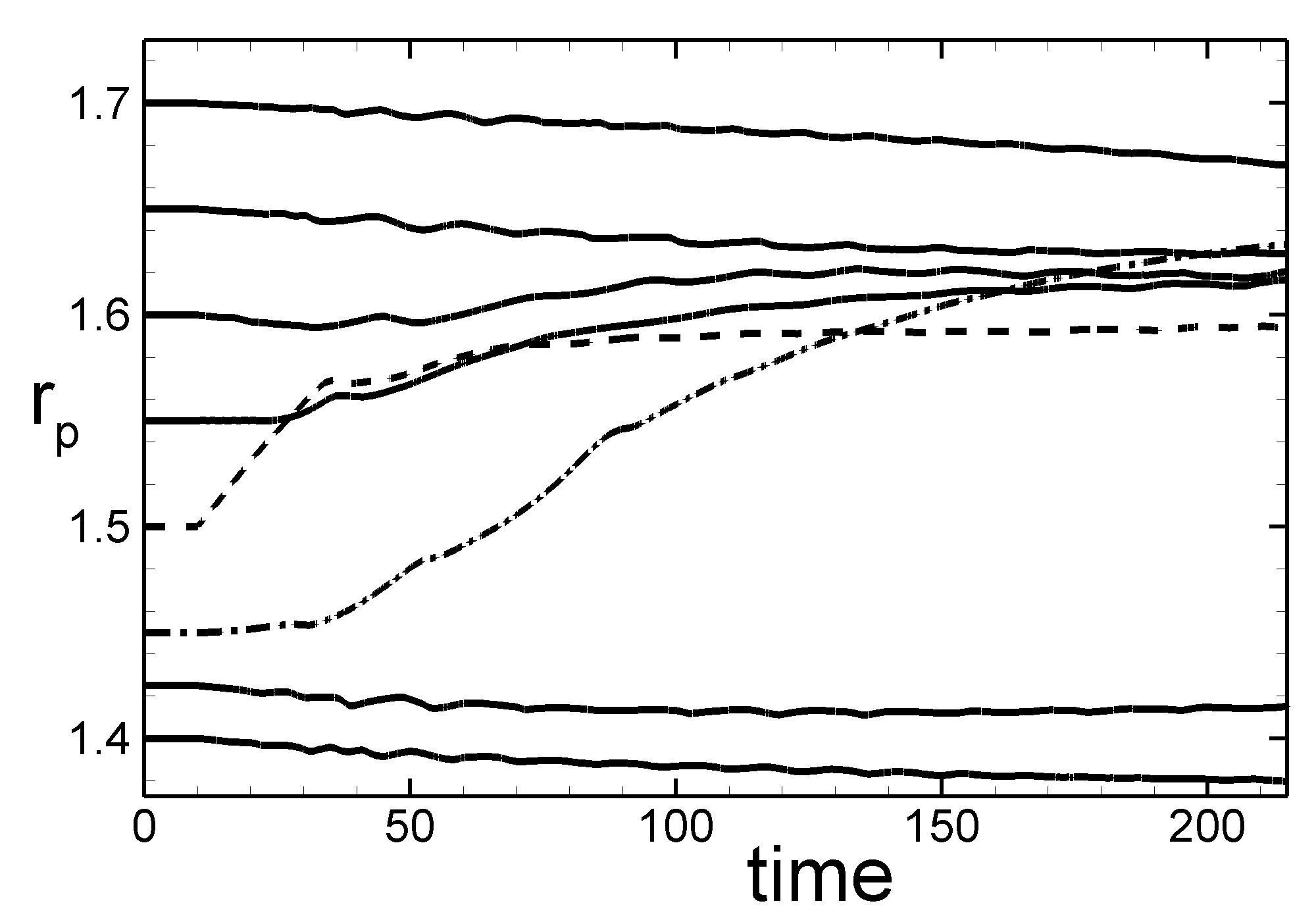
Figure 3: Migration tracks for planets of mass $M_{p}=5M_{\oplus}$ and initial orbital radii in the range of $r_{p}$ = 1.4–1.7. Tracks that start at $r_{p}=1.45$ and $r_{p}=1.5$ are shown as dashed and dash-dotted lines.

4 Results

Initially, the transition between the disc and cavity is very sharp (see top panel of Fig. 1). However, our equilibrium is not precise, and the density in the disc has been slightly redistributed during the first 10-20 rotations. The density redistribution led to a smoother distribution at the disc-cavity boundary (see middle panel of the same figure). Later on, the density distribution in the disc varied only slightly over time (see the middle and bottom panels corresponding to $t=20$ and $t=100$, respectively). The right panel of Fig. 1 shows the linear distribution of the $\phi-$averaged surface density at $t=0,20,50$ and $100$.

The planet is initialized on a fixed circular orbit; the disc is allowed to relax from $t$ = 0 to $t=10$ before the planet is released and permitted to migrate. We place a planet in different parts of the disc, in the cavity and in the disc-cavity boundary, and investigate its migration.

4.1 Migration in the inner disc

First, as a test case, we model the migration of planets in the inner disc, where the surface density is approximately constant. We placed a planet at an initial radius of $r_{p}=2$, away from the disc-cavity boundary, and observed a slow inward migration towards the star.

The migration path of a planet is mainly determined by the Lindblad and corotation torques (Goldreich & Tremaine, 1979, 1980; Ward, 1986; Artymowicz, 1993a; Ward, 1997). The Lindblad torque is generated when a planet excites $m$-armed waves in the disc with “orbital” frequencies $\omega=m\Omega_{\rm p}$. The dispersion relation for these waves in a low-temperature, low-mass disc is $\left(\omega-m\Omega\right)^{2}=\kappa^{2},$ where $\kappa=\Omega_{\rm Kep}$ is the epicyclic frequency in a Keplerian disc. Substituting $\Omega(r)~{}=~{}\sqrt{{GM_{\star}}/{{r^{3}}}}$, the locations of the Lindblad resonances are :

$$r_{\rm LR}=r_{\rm p}\left(\frac{m\pm 1}{m}\right)^{2/3}.$$ (10)

Fig. 2 shows that a planet generates two spiral density waves in the disc. It also shows the position of the low-order Lindblad resonances. The lowest order outer Lindblad resonances (OLR) are located at $r_{\rm OLR,m=1}\approx 1.59r_{p}\approx 3.18$, $r_{\rm OLR,m=2}\approx 1.31r_{p}\approx 2.62$, $r_{\rm OLR,m=3}\approx 1.21r_{p}\approx 2.42$, etc. All of them are located in the disc and exert a negative torque on the planet. The lowest-order inner Lindblad resonance (ILR), $r_{\rm ILR,m=2}\approx 0.63r_{p}\approx 1.26$, is located inside the low-density cavity, while the higher order resonances, $r_{\rm ILR,m=3}\approx 0.76r_{p}\approx 1.52$, $r_{\rm ILR,m=4}\approx 0.82r_{p}\approx 1.65$, etc., are located at the disc-cavity boundary and in the disc. They exert a positive torque on the planet. The torque from the OLR is larger in magnitude, causing the overall cumulative torque to be negative. This drives the inward migration of the planet. Note that the torque per unit radius increases with $m$, and the cumulative torque is determined by the Lindblad resonances with high $m-$numbers (e.g. Goldreich & Tremaine 1980).

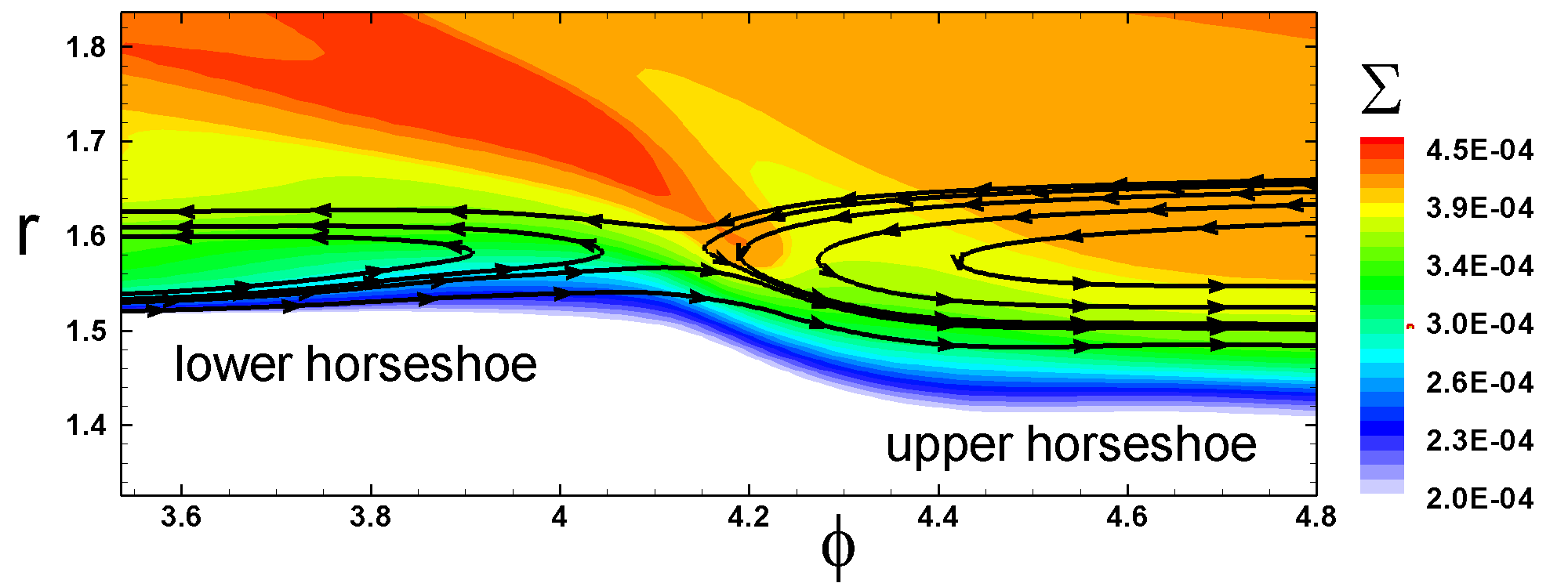
Figure 4: The horseshoe orbits of gas around a planet of mass $15M_{\oplus}$, located at the disc-cavity boundary. The colour background shows surface density.

The corotation torque arises from the material in the planet’s co-orbital region where $\Omega\approx\Omega_{p}$. The physics of the corotation torque and its effect on planet migration have been studied by a number of authors both theoretically and numerically (e.g. Goldreich & Tremaine 1979; Ward 1991; Ogilvie & Lubow 2003, 2006; Masset & Ogilvie 2004; Paardekooper & Mellema 2006; Baruteau & Masset 2008; Paardekooper & Papaloizou 2009a; Kley et al. 2009; Masset & Casoli 2009, 2010; DÁngelo & Lubow 2010; Paardekooper et al. 2010, 2011; Paardekooper 2014).

The co-orbiting material undergoes a horseshoe-shaped orbits in the vicinity of the planet and asymmetries in the corotation region lead to exchange of angular momentum between the planet and the disc matter (e.g. Ward 1991). Goldreich & Tremaine (1979) used the linear approximation and calculated the corotation torque as a superposition of torques from waves excited in the corotation region. They have shown that the value and the sign of the corotation torque strongly depend on the sign of the local density gradient.

Tanaka et al. (2002) used the linear approximation to calculate both the Lindblad and the corotation torques in 2D and 3D isothermal discs, and obtained the total torques as follows:

$$\noindent\Gamma_{\rm(L+C),3D}=-(1.364+0.541s)\Gamma_{0}~{},$$ (11)

$$\Gamma_{\rm(L+C),2D}=-(1.160+2.828s)\Gamma_{0}~{},$$ (12)

where $\Gamma_{0}=({q_{p}}/{h})^{2}\Sigma_{p}r_{p}^{4}\Omega_{p}^{2}$. Here, $\Sigma_{p}\sim r^{-s}$ is the surface density in the disc at the orbital radius of the planet, $r=r_{p}$. In 3D isothermal discs, the total torque becomes positive (and the planet migrates outward) if $(1.364+0.541s)<0$, that is, at condition $s<-2.52$, which corresponds to a high positive density gradient. In 2D discs, the condition is $s<-0.41$. In our disc, the surface density distribution is flat, $s=0$, the total torque is negative, and the planet migrates inward. Overall, we observed typical type I migration similar to that observed by other authors who performed 2D or 3D simulations (see, e.g., review paper by Kley & Nelson 2012 and references therein).

4.2 Migration at the disc-cavity boundary

Next, we study the migration of planets at the disc-cavity boundary. For that, we place a planet in different parts of the disc-cavity boundary and its vicinity and study its migration.

Fig. 3 shows the migration tracks of planets with mass $M_{p}=5M_{\oplus}$, which start at different radii $r_{p}$ from the star, ranging from $r_{p}=1.4$, which corresponds to the low-density cavity, to $r_{p}=1.7$, which corresponds to the inner part of the disc. This figure shows that the planets starting just outside the disc-cavity boundary (at $r_{p}$ = 1.65 and $r_{p}$ = 1.7) migrate inward due to differential Lindblad torque, which is analogous to the migration in the disc discussed in Sec. 4.1. The torque is mainly determined by the OLR, because many of the ILR are located in the low-density cavity. The torque is negative and the planets migrate inward. Later on, they stop migrating because they reach the regions of large positive density gradient, where the corotation torque is high, and their migration stops due to the balance of the torques.

Planets that start migrating from a region of high density gradient ($r_{p}=1.45,1.5,1.55$) migrate rapidly outward. Later on, when they reach the parts of the disc with a lower density gradient, their migration slows down and stalls at the radius where the positive corotation torque is balanced by the negative Lindblad torque.

Figure 5: Torque profiles. Top panels: torque per unit disc mass for planets with masses $5M_{\oplus}$ and $15M_{\oplus}$, located at distances $r_{p}=1.5$ and $1.7$ from the star, at $t=20$. Bottom panels: cumulative torque as a function of normalized radius.

Fig. 3 shows that the orbits of the planets migrating from smaller and larger radii converge at the radius of $r_{\rm trap}\approx 1.6$, which corresponds to the planet trap radius. This analysis shows that there is a stable halting region where the positive corotation torque balances the negative differential Lindblad torque, and therefore the planet is trapped.

In another set of numerical experiments, we studied the migration of planets with mass $M_{p}=15M_{\oplus}$ and observed a similar convergence of migration paths at the radius of $r_{\rm trap}\approx 1.65$. However, the planets migrated approximately three times faster, which is in agreement with the dependence for the migration time scale, $\tau\sim M_{p}^{-1}$, derived from theoretical studies (see, e.g. Eq. 70 of Tanaka et al. 2002).

The corotation torque is associated with the asymmetry of the horseshoe shaped orbits of matter near a planet (Ward, 1991). Namely, in the coordinate system of the planet, the co-orbital matter performs U-turns near the planet, such that the matter in front of the planet transfers its angular momentum to the planet, while the matter behind the planet takes angular momentum away from the planet.

Fig. 4 shows an example of the strong asymmetry of the horseshoe orbits around a planet with mass $M_{p}=15M_{\oplus}$, located in the region of the high density gradient ($r_{p}\approx 1.5$). One can see that matter in the upper horseshoe (located at the right side of the plot) carries more mass (and angular momentum) than the lower horseshoe (left side of the plot). Matter comes to the upper horseshoe orbits from the high-density disc (located above the planet in the plot), while matter to the lower horseshoe comes from the low-density cavity (located below the planet in the plot). The positive torque associated with the upper horseshoe is much larger than the negative torque associated with the lower horseshoe, and the planet migrates outward.

To investigate the asymmetry of the torques acting at the disc-cavity boundary, we calculated the torque per unit disc mass (e.g. Masset et al. 2006a; DÁngelo & Lubow 2008):

$$\frac{d\Gamma_{z}}{dM}=\frac{1}{2\pi\Sigma_{\rm avg}}\int_{-\infty}^{\infty}\int_{0}^{2\pi}\gamma_{z}d\phi dz~{}$$ (13)

as a function of normalized radius $(r-r_{p})/r_{p}$, where

$$\gamma_{z}=\rho(\mathbf{x})\frac{\partial\Phi_{p}}{\partial\phi}=\frac{GM_{p}\rho(\mathbf{x})}{(|\mathbf{x}-\mathbf{x_{p}}|^{2}+\epsilon^{2})^{3/2}}rr_{p}\sin(\phi-\phi_{p})~{}$$ (14)

is the torque per unit volume (torque density) acting on the planet from the disc, and $\Phi_{p}$ is the gravitational potential of the planet (second term in Eq. 8). The top panels of Fig. 5 show torque per unit mass for planets with masses $M_{p}=5M_{\oplus}$ and $M_{p}=15M_{\oplus}$. The bottom panels of the same figure show the cumulative torque, i.e., the torque density integrated over a given radius.

Fig. 5 shows that, for a planet that migrates from radius $r_{p}=1.7$ (dashed line), both the inner and outer Lindblad resonances contribute to the torque on the planet. The total torque from the OLR is larger in magnitude, causing the cumulative torque to be negative. This drives inward migration of the planet, as shown in Fig. 3. For a planet at $r_{p}=1.5$, there is a strong positive torque from the region interior to the planet, resulting in a large positive cumulative torque (bottom panels). This large, positive torque causes the planet to migrate rapidly outward.

The degree of asymmetry between the torques sets the direction of the planet’s overall migration. This net torque can be measured by integrating the torque density over the simulation region:

$$\Gamma_{z}=\int_{\mathcal{V}}{\gamma_{z}}dV=GM_{p}\int_{\mathcal{V}}{\rho(\mathbf{x})\frac{rr_{p}\sin(\phi-\phi_{p})}{(|\mathbf{x}-\mathbf{x_{p}}|^{2}+\epsilon^{2})^{3/2}}dV}~{}.$$ (15)

We calculated the time-averaged torque (during the time interval of $t=10-60$) acting on the planets located at different distances $r_{p}$ from the star. Fig. 6 shows that the positive torque on the planets at the disc-cavity boundary (red triangles) is much larger than the negative torque acting in the disc or cavity. This contrast shows how powerful the trapping mechanism is: the planets that try to migrate into the cavity enter the region of a high positive density gradient and experience strong positive torque, which prevents them from migrating. One can see that the torque is zero at $r_{\rm trap}\approx 1.6$ and $r_{\rm trap}\approx 1.65$ for planets with masses $M_{p}=5M_{\oplus}$ and $M_{p}=15M_{\oplus}$, respectively. Planets in these regions are stably trapped, because the torque interior to $r_{\rm trap}$ is positive and drives outward migration towards the trap; similarly, the torque exterior to $r_{\rm trap}$ is negative and also drives inward migration towards the trap. Overall, these 3D simulations confirm the results of the earlier studies by Masset et al. (2006a) and Morbidelli et al. (2008), who predicted the existence of stable planet traps in their 2D simulations. Below, we compare results of our 3D simulations with results obtained in theoretical studies and 2D simulations.

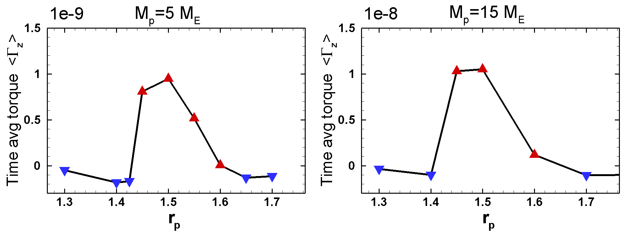
Figure 6: The time-averaged total torque. The plot shows $\left<\Gamma^{\rm tot}_{z}\right>$ versus planet radius $r_{p}$ for the planets with initial orbits near the disc-cavity boundary. The torques are computed by time averaging between $t$ = 10 (when the planet is first allowed to migrate) and $t$ = 60. Left and right panels show the torques for planets with masses $M_{p}=5M_{\oplus}$ and $M_{p}=15M_{\oplus}$, respectively.

4.3 Non-linear horseshoe drag and the width of the horseshoe region

The corotation torque associated with horseshoe orbits has been calculated in general, non-linear approach by Ward (1991) in 2D isothermal discs as:

$$\Gamma_{\rm HS}=\frac{3}{4}\Sigma_{p}\Omega_{p}^{2}x_{s}^{4}\bigg{[}\frac{d{\rm log}(\Sigma/B)}{d{\rm log}r}\bigg{]}~{},$$ (16)

where $B=(1/2r)d(r^{2}\Omega)/dr$ is vorticity, and $B/\Sigma$ is specific vorticity (or vortencity). The torque depends strongly on the half-width of the horseshoe region, $x_{s}$. For low-mass planets (where $q_{p}<<h^{3}$) located in isothermal discs, $x_{s}$ has been estimated as:

$$x_{s}\approx k_{s}r_{p}\sqrt{q_{p}/h}~{},$$ (17)

where slightly different values of $k_{s}$ were found in different studies: $k_{s}=0.96$ (Masset, 2001) and $k_{s}=1.16$ (Masset et al., 2006b; Paardekooper & Papaloizou, 2009b).

We can find the values of $x_{s}$ and $k_{s}$ from our simulations. Fig. 7 shows streamlines of matter flow around a planet of mass $5M_{\oplus}$, with its initial location at $r_{p}=1.5$, at different moments in time: $t=20,100,150,200$. Initially, at $t=20$, the planet is located at the steep part of the density slope, and the horseshoe orbits are strongly asymmetric. Later on, a planet moved to larger radius, $r_{p}\approx 1.6$, where the density gradient is not as high, and orbits become somewhat more symmetric. However, in all cases the upper and lower horseshoe orbits originate in the regions of high and low density, respectively, which provides asymmetry in the corotation torque. From Fig. 7, we find the approximate value of the observed width of the horseshoe region, $\Delta r\approx 0.11$ and obtain $x_{s}=0.5\Delta r/r_{p}\approx 0.034$. Using this value, and taking $r_{p}=1.6$, $q_{p}=1.5\times 10^{-5}$ and $h=0.03$, we obtain $k_{s}\approx 0.95$. This value is in agreement with earlier findings .

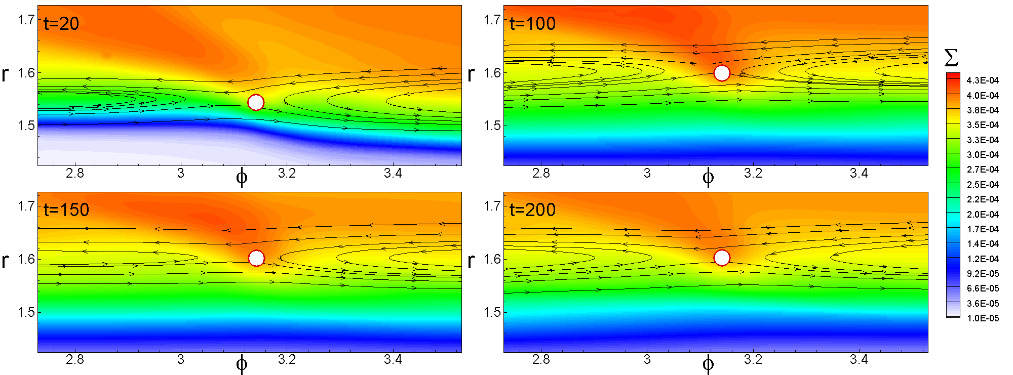
Figure 7: Streamlines of matter flow around a planet of mass $5M_{\oplus}$ with initial location at $r_{p}=1.5$ at $t=20,100,150,200$. The colour background shows the surface density, $\Sigma$. The circle shows the position of the planet (not to scale).

4.4 Saturation of the corotation torque

The horseshoe corotation torque is prone to saturation, because a planet exchanges angular momentum with the co-orbital matter, which cannot transfer the angular momentum to other parts of the disc unless new matter enters the corotation region due to viscosity or some other mechanism (e.g. Ward 1991; Masset 2001; Masset & Ogilvie 2004; Ogilvie & Lubow 2006). Saturation will not occur if new matter enters the horseshoe region with the time scale smaller than the libration time scale (Masset, 2001, 2002):

$$\tau_{\rm lib}=\frac{8\pi}{3{\bar{x}}_{s}}\Omega_{p}^{-1}~{},$$ (18)

during which a fluid element at the orbital radius $r_{p}(1+{\bar{x}}_{s})$ completes two orbits in the frame corotating with the planet. The disc turbulence, which provides an effective viscosity, can help to prevent the corotation torque from saturation. In our model we switched the module of viscosity off, which helped us to support the same density distribution at the disc-magnetosphere boundary .

However, in our model, the saturation does not occur, because planets migrate rapidly, so that new matter comes into the horseshoe region due to the planet’s migration (e.g. Paardekooper et al. 2010; Paardekooper 2014). The torque will stay unsaturated, if the time scale of migration through the region $2x_{s}$ is smaller than the libration time scale: $2x_{s}/{\dot{r}}_{p}<\tau_{\rm lib}$. The corresponding migration rate is:

$$\dot{r}_{p}\gtrsim 1.33\times 10^{-4}\bigg{(}\frac{r_{p}}{1.5}\bigg{)}^{1/2}\bigg{(}\frac{M_{p}}{5M_{\oplus}}\bigg{)}\bigg{(}\frac{h}{0.03}\bigg{)}^{-1}~{}.$$ (19)

In application to our model, we obtain: ${\dot{r}}_{p}\gtrsim 1.33\times 10^{-4}$ and $\dot{r}_{p}\gtrsim 4.0\times 10^{-4}$ for planets with masses $M_{p}=5M_{\oplus}$ and $M_{p}=15M_{\oplus}$, respectively . We compare this rate with the migration rate observed in simulations. Fig. 8 shows the migration rates obtained from simulations for planets with mass $M_{p}=15M_{\oplus}$ . The measured migration rates at the disc-cavity boundary, ranging as $\dot{r_{p}}=3\times 10^{-3}-4\times 10^{-4}$, are comparable or larger than the critical value (obtained from Eq. 19), and therefore the corotation torque is not saturated.

When the planet reaches the position of zero torque ($r_{p}\approx 1.6-1.65$) the migration stalls, and the corotation torque can be saturated. However, at the disc-cavity boundary, the conditions for saturation may be different compared with other parts of the disc. Namely, the processes which support the disc-cavity boundary, will also support the asymmetry of the horseshoe orbits, and would prevent the saturation of corotation torque. For example, in cases of the disc-magnetosphere boundary, the density in the disc is always larger than the density in the cavity. The balance between the matter pressure in the disc and the magnetic pressure in the cavity establishes rapidly, on a time scale comparable with the Keplerian rotation at the boundary (e.g. Romanova et al. 2003; Blinova et al. 2016), which is much shorter than the libration time scale. Therefore, a sharp density gradient and asymmetry of the horseshoe orbits would always be supported at the boundary, and therefore high viscosity or rapid migration are not required to prevent the corotation torque from saturation. In cases of disc-cavity boundaries of different origins, the details of saturation depend on the physics of these boundaries and should be studied separately.

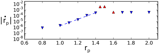
Figure 8: Absolute value of the migration rates of a planet of mass $M_{p}=15M_{\oplus}$, with initial orbital radii ranging from $r_{p}$ = 0.8–2.0. The downward pointing (in blue) triangles indicate inward migration, while the upward pointing triangles (in red) indicate outward migration.

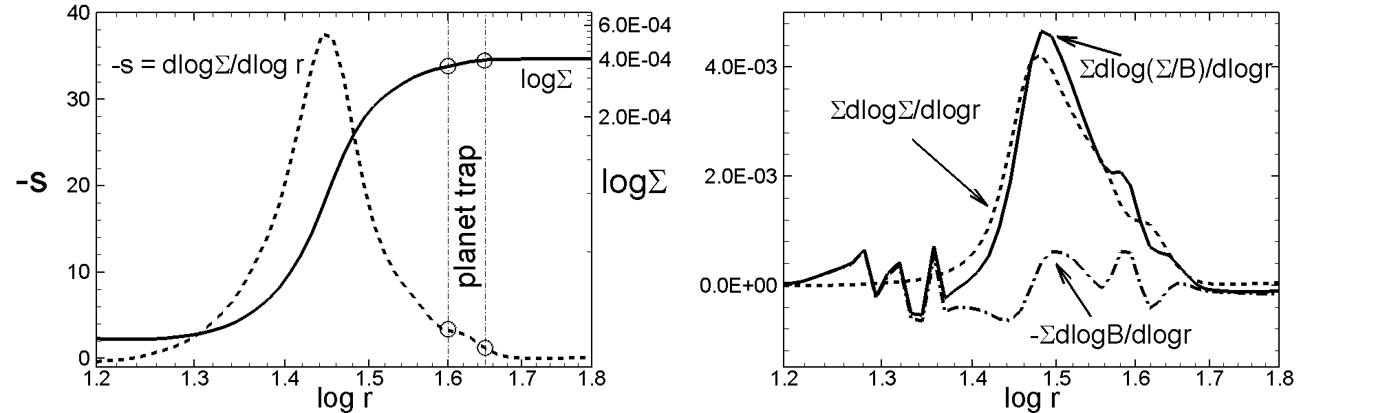
Figure 9: Left panel: The radial distribution of the azimuthally-averaged surface density, $\Sigma$ (solid line), and the power in the density distribution, $-s=d{\rm log}\Sigma/d{\rm log}r$. Vertical lines and small circles show the range of parameters at which the low-mass planets are trapped. Right panel: Components of the horseshoe torque associated with the density gradient (dashed line), with the gradient of vorticity, $B$ (dash-dot line), and the total torque (solid line).

4.5 Comparisons with 2D simulations of planet trapping

Masset et al. (2006a) considered the migration of low-mass planets of $1-15M_{\oplus}$ at the disc-cavity boundary, where the disc and the cavity have uniform surface densities of $\Sigma_{o}$ and $\Sigma_{i}$, respectively. They supported this configuration, placing different values of $\alpha-$parameter of viscosity in the disc and in the cavity ($\alpha=10^{-4}$ and $\alpha=10^{-2}$, respectively), which helped them to evacuate matter from the cavity in steady-state fashion. Compared with their simulations, we consider inviscid discs, where the quasi-steady disc-cavity configuration is supported for a long time due to very low (numerical) viscosity.

Masset et al. (2006a) considered the disc-cavity boundaries with the width of the transition region, $\lambda\approx 4H<<r$, and density ratios between the disc and the cavity of $\Sigma_{d}/\Sigma_{\rm cav}=7$ and $1.4$. In our simulations, we have similar width of the transition region, $\lambda\approx 0.2\approx 4.4H$, but larger density ratio between the disc and the cavity, which is $\rho_{d}/\rho_{\rm cav}=100$ in the equatorial plane, which corresponds to $\Sigma_{d}/\Sigma_{\rm cav}\approx 14$ for surface densities.

Masset et al. (2006a) noted that, in the transition region, the term $d\rm{log}\Sigma/d\rm{log}r$ is a sharply peaked function with a maximum that scales as $|{d\rm{log}\Sigma}/{d\rm{log}r}|_{\rm max}\sim{r}/{\lambda}\rm{log}({\Sigma_{o}}/{\Sigma_{i}})~{}.$ The left panel of Fig. 9 shows typical surface density distribution in our model and the distribution of the power $-s=d\rm{log}\Sigma/d\rm{log}r$ with radius. One can see that $-s$ has small values at the edges of the disc-cavity boundary, but is sharply peaked at $-s\approx 36$ in the middle of the boundary, at $r\approx 1.45$.

Masset et al. (2006a) analyzed the radial distribution of the main terms in the horseshoe corotation torque, $\Gamma_{C}\sim\Sigma{d\rm{log}(\Sigma/B)}/{d{\rm log}r}~{}$:

$$\Sigma\frac{d\rm{log}(\Sigma/B)}{d{\rm log}r}=\Sigma\frac{d\rm{log}\Sigma}{d{\rm log}r}-\Sigma\frac{d\rm{log}B}{d{\rm log}r}~{},$$ (20)

where the left and right terms are associated with the surface density gradient and the vorticity gradient, respectively. Masset et al. (2006a) compared these two terms and concluded that they are comparable and both contribute to the corotation torque (see Fig. 1 from Masset et al. 2006a).

We also calculated and compared these terms, taking one of our models, where a planet of mass $5M_{\oplus}$ started its migration at $r_{p}=1.55$ and migrated outward. The right panel of Fig. 9 shows these terms separately and their sum at the moment of time corresponding to $t=100$. One can see that the density gradient term is much larger than the gradient of vorticity term. This can be explained by the fact that in our model the density gradient at the disc-cavity boundary is larger than that in the model of Masset et al. (2006a).

Masset et al. (2006a) observed that planets migrating from the disc halt their migration at the edge of the disc, before entering the low-density cavity. In our simulations we also observed that the migration halts at the disc edge, before entering the sharp boundary, though we considered the migration from either side, from the disc or from inside the boundary.

From the left panel of Fig. 9, we see that the trapping region is located in parts of the disc with relatively small positive density gradients. Left and right vertical lines show the positions of the planet trap, $r_{\rm trap}\approx 1.6$ and $r_{\rm trap}\approx 1.65$, for planets with masses of $5M_{\oplus}$ and $15M_{\oplus}$, respectively. The density gradients are $-s=3.3$ and $-s=1.2$, respectively. These values approximately correspond to the value of $s\approx-2.52$ for zero torque in Eq. 12 from Tanaka et al. (2002) for 3D discs .

Note that a large density drop is not necessary for planet trapping: simulations show that planets are trapped at the parts of the disc with relatively small values of the positive density gradient (see also Sec. 4.7).

Overall, our 3D simulations confirm the trapping mechanism proposed and studied by Masset et al. (2006a) in 2D simulations. Our Fig. 6 and Fig. 1 from Masset et al. (2006a) show that the positive corotation torque strongly increases when a planet moves away from its trapping location towards the disc-cavity boundary, and therefore the boundary represents a stable trap for the low-mass planets.

4.6 Comparisons with 2D models of adiabatic discs

In our simulations, we used the adiabatic equation of state . Below, we compare results of our 3D simulations with 2D simulations of Paardekooper et al. (2010), who studied torques acting on the low-mass planets in case of non-isothermal, adiabatic discs. In their 2D model, no density jumps were considered, but instead the surface density, temperature and entropy smoothly vary with radius as

$$\Sigma\sim r^{-s},~{}T\sim r^{-\beta},~{}S\sim r^{-\xi~{}}.$$ (21)

From their simulations, they derived analytical dependencies for the linear Lindblad torque and non-linear (horseshoe) corotation torque (see their equations 14 and 45) as

$$\gamma\Gamma_{L}/\Gamma_{0}=-(2.5+1.7\beta-0.1s){\bar{b}}^{0.71}~{},$$ (22)

$$\gamma\Gamma_{C}/\Gamma_{0}=1.1{\bar{b}}\bigg{(}\frac{3}{2}-s\bigg{)}+\frac{\xi}{\gamma}{\bar{b}}\bigg{(}10.1\sqrt{\bar{b}}-2.2\bigg{)}~{},$$ (23)

where ${\bar{b}}=0.4/(b/h)$, $b$ is the softening parameter in the equation for the potential of the star-planet system. The left and right terms in the right-hand side of eq. 23 for the corotation torque are connected with the vortencity and entropy gradients, respectively.

For comparisons with our model, we take the value of softening $\epsilon=0.025$, used in our model, and obtain $b=\epsilon/r_{p}=0.025/r_{p}\approx 0.0167$ (at $r_{p}=1.5$) and $\bar{b}=0.4/(b/h)\approx 0.72$. We also take into account that in adiabatic discs $\beta=\xi+(\gamma-1)s~{}$ and take the value $\gamma=5/3$ used in our model, and obtain the total torque in the form:

$$\gamma\Gamma_{(L+C)}/\Gamma_{0}=-0.79-1.61s+1.40\xi~{}.$$ (24)

In cases of steady cold discs (which are in the force equilibrium) the pressure gradient force is small and pressure varies only slowly with radius. Then from the ideal gas equation, one obtains $\beta\approx-s$, and $\xi=\beta-(\gamma-1)s\approx-\gamma s$. Substituting these values to Eq. 24, one obtains that the torque is positive, if $s\lesssim-0.2$.

To compare our 3D model with the above 2D model, we integrate different values obtained in our model in z-direction and obtain surface density, $\Sigma$, surface pressure, $\Pi$, surface temperature, $T^{\prime}$ and surface entropy, $S^{\prime}$. Fig. 10 shows typical radial distribution of these values at the disc-cavity boundary. One can see that the surface pressure is almost constant, as expected, so that the quasi-steady state is supported across the boundary. The surface entropy $S^{\prime}=\Pi/\Sigma^{\gamma}\approx\Sigma^{-\gamma}\sim r^{\gamma s}$ decreases with radius. The surface temperature is connected with pressure and density through an ideal gas law: $T^{\prime}=\Pi/\Sigma$ (in our dimensionless units), and is approximately inverse function of the surface density, $T^{\prime}\sim\Sigma^{-1}\sim r^{s}$.

Our simulations show that the migration of planets halts at radii $r\approx 1.6-1.65$. From Fig. 10 we derive the slope in the surface density distribution in the interval of radii of $1.6<r<1.65$ and obtain an approximate value of $s\approx-(2.0-2.3)$. This value is larger than the value obtained from the theoretical estimates, $s\approx-0.2$. The difference may be due to the fact that our simulations are three-dimensional, while the comparisons were performed for two-dimensional discs. For example, in cases of isothermal discs, Tanaka et al. (2002) obtained zero torque at $s\approx-0.41$ for 2D discs, and $s\approx-2.52$ for 3D discs. We suggest that in cases of adiabatic discs, the zero-torque value of $s$ can be also different in 3D discs versus 2D discs.

Figure 10: The radial distribution of the azimuthally-averaged values at the disc-cavity boundary at $t=100$: the surface density, $\Sigma$ (solid line), surface pressure, $\Pi$ (dash-dot line), surface entropy $S^{\prime}$ (solid line), and surface temperature, $T^{\prime}$ (dashed line).

4.7 Minimum density drop for planet trapping

In our model, the surface density ratio between the disc and cavity is high, $\Sigma_{d}/\Sigma_{\rm cav}\approx 13.6$. Such a high density ratio is not necessary for trapping. In this section we estimate the minimum density ratio which is necessary for trapping.

Our simulations show that planets are trapped at the edge of the disc, before reaching the sharp density drop at the disc-cavity boundary. They are trapped in parts of the disc where the positive density gradient $-s\approx 3.3$ for $M=5M_{\oplus}$ and $-s\approx 1.2$ for $M=15M_{\oplus}$. Tanaka et al. (2002) found from semi-analytical studies, that the positive corotation torque balances the negative Lindblad torque (when a planet can be trapped) at $-s=2.52$ (in the case of 3D discs).

To estimate the minimum density drop, which is needed for trapping, we consider a cavity with a linear distribution of the surface density, which varies from $\Sigma_{d}$ in the disc at $r=r_{d}$ to $\Sigma_{\rm cav}$ in the cavity at $r=r_{\rm cav}$. Then we can write the power $s$ in the surface density slope as

$$-s=\frac{d{\rm log}\Sigma}{d{\rm log}r}=\frac{\Delta{\rm log}\Sigma}{\Delta{\rm log}r}=\frac{{\rm log}(\Sigma_{d}/\Sigma_{\rm cav})}{{\rm log}(r_{d}/r_{\rm cav})}~{}.$$ (25)

One can see that the power $s$ depends on the density drop, $\Sigma_{d}/\Sigma_{\rm cav}$, and also on the ratio $r_{d}/r_{\rm cav}=1/(1-\Delta r/r_{d})$, where $\Delta r=r_{d}-r_{\rm cav}$ is the width of the transition region. Using these approximations, we can estimate the density drop. For example, in our simulations $r_{d}\approx 1.6$, $r_{\rm cav}\approx 1.4$, $\Delta r\approx 0.2$, $\Delta r/r_{d}=0.125$ and $r_{d}/r_{\rm cav}\approx 1.143$. Then for values of $-s=1.2$ and $-s=3.3$ we obtain $\Sigma_{d}/\Sigma_{\rm cav}\approx 1.2$ and $1.6$, respectively. If we take $-s=2.52$ from Tanaka et al. (2002) (see Eq. 12) then we obtain $\Sigma_{d}/\Sigma_{\rm cav}\approx 1.4$. These estimates show that a small density drop is sufficient for trapping low-mass planets. We note that Masset et al. (2006a) tested the trapping region with the density drop of $\Sigma_{d}/\Sigma_{\rm cav}\approx 1.4$ in their 2D simulations and observed planet trapping.

5 Applications

A planet can be trapped at the disc-cavity boundaries, which are expected in several places of the protoplanetary discs.

5.1 A planet trap at the disc-magnetosphere boundary

Young low-mass stars at the centers of protoplanetary systems tend to be highly magnetized due to the onset of convection in their protostellar cores (e.g. Donati & Landstreet 2009). The stellar field truncates the inner disc, creating a low-density magnetospheric cavity, where the matter ram pressures in the disc balances the magnetic pressure of the stellar field (e.g. Königl 1991). This density transition between the low-density magnetosphere and the higher-density accretion disc has a sharp positive density gradient due to the truncation by the magnetic field (e.g. Romanova et al. 2002, 2003; Romanova & Lovelace 2006.

A migrating planet which encounters this boundary becomes trapped due to this sharp density gradient at the disc-magnetosphere interface. For a typical T Tauri star, the magnetospheric boundary is located at $\sim 0.05-0.1$ AU and may serve as the final barrier, preventing planets from migrating all the way into their host stars. The accretion rates in the disc around young stars may span several orders of magnitude, from $\dot{\rm M}\sim 10^{-7}-10^{-11}{\rm M}_{\astrosun}/{\rm yr}$, meaning that the size of the magnetospheric cavity can also differ substantially between young stellar systems (e.g. Hartmann 2000).

If the disc accretion rate declines and the magnetospheric radius increases, the trapped planet will move outward with the inner edge of the disc due to the action of the corotation torque (Masset et al., 2006a; Liu et al., 2017). Liu et al. (2017) suggested that this mechanism may be responsible for the dispersal of low-mass planets at $r\lesssim 1$ AU and their observed nearly homogeneous distribution with periods.

5.2 A planet trap at the dust sublimation radius and at the dead zone

Observations of protoplanetary discs show an infrared excess at 3 $\mu$m, which can be attributed to an inner disc edge at a distance coinciding with the dust-sublimation radius of the system (Dullemond et al., 2001). Exterior to this radius, the disc is cold and dusty, and the MRI-powered accretion (which is sensitive to the ionization fraction in the disc) proceeds slowly.

However, interior to the dust sublimation radius, the gas disc is optically thin and the ionization fraction is high. As a result, the viscosity provided by the MRI turbulence is large and accretion interior to the dust sublimation radius proceeds efficiently. The result is an evacuated low-density inner cavity surrounded by a cold, higher density disc. Migrating planets which encounter this inner cavity may become trapped at the density transition and migrate in or out if the dust sublimation radius changes as the young star moves along the Hayashi track towards the main sequence.

Infrared observations of protoplanetary discs show that these inner cavities can range from $\sim$0.1 to 4 AU in size, depending on the luminosity of the star (Muzerolle et al., 2003; Akeson et al., 2005; Monnier et al., 2005). The outer edge of this cavity may act as a trap for inwardly migrating planetesimals, allowing for the gradual buildup of planetary embryos in this region (Morbidelli et al., 2008).

The low-mass migrating planets may also become trapped at the inner edge of a dead zone (Gammie, 1996; Matsumura et al., 2007; Guilera & Sándor, 2017), where the ionizing radiation does not penetrate far enough into the disc to sustain MRI-driven accretion (Masset et al., 2006a). The surface density in the dead zone is expected to be substantially higher than the density in the inner regions, where the MRI-driven turbulence is ongoing. As such, the inner edge of the dead zone may serve as a trap for migrating planets. Like the dust sublimation radius, the inner dead zone radius may change in time, causing planets trapped at the inner edge to move in or out correspondingly (Masset et al., 2006a; Kretke & Lin, 2012).

5.3 Planet traps at snow lines

The positive density gradients can also form at snow lines, associated with the phase transition from liquid to frozen states. Each molecular species has its own condensation front, depending on its unique freeze-out temperature, and therefore several snow lines are expected in protoplanetary discs. At the snow line, a sudden change in viscosity is expected due to a sharp increase in the grain-to-dust density ratio, and the changes of the turbulence properties (driven by MRI).

The snow lines associated with freezing of water are the closest to stars and are expected to be at distance of several AU (e.g. Kretke & Lin 2007). The positive density gradient and the corresponding corotation torque can stop Type I migration of several Earth mass cores (Zhang et al., 2007), which are necessary for the formation of giant planets (Pollack et al., 1996) and their survival at 2-3 AU.

Recently, the $\sim 30$ AU snow line associated with the freezing of CO molecules has been resolved in T Tauri star TW Hya by ALMA telescope (e.g. Qi et al. 2013), which was a proof that snow lines are a prominent features in protoplanetary discs.

Note that at the snow lines, and other types of disc-cavity boundaries, the positive corotation torque can also be connected with the negative entropy gradient (e.g. Paardekooper & Mellema 2006; Kley & Crida 2008; Kley et al. 2009; Paardekooper & Papaloizou 2009c; Hasegawa & Pudritz 2011; Lega et al. 2014). This is an additional physical mechanism which may stop migration of planets at the disc-magnetosphere boundary.

6 Conclusions

We present global 3D simulations of low-mass planets migrating near the edge of a disc cavity. The main points of this study are as follows:

• For planets migrating far from the cavity boundary, the migration proceeds due to the excitation of density waves at the Lindblad resonances. However, migrating planets which encounter the boundary experience a large positive corotation torque due the the positive surface density gradient at the disc-cavity interface.

• There exists a region in the disc where the magnitude of the corotation torque is equal and opposite to the differential Lindblad torque, resulting in a region where a planet experiences zero net torque from the disc. Interior to this region, the net torque is positive due to the corotation torque and the planet migrates outward; similarly, exterior to this location, differential Lindblad torque is larger in magnitude and the net torque is negative, resulting in inward migration. Hence the zero-torque region is a stable “planet trap” as any perturbations in either direction result in a torque which pushes the planet back toward the trapping region.

• An accretion disc around a young star may have several planet traps wherever there is a large positive surface density gradient in the disc. Such density gradients may appear at the edge of the magnetospheric cavity, at the inner edge of the dead zone, at the dust-sublimation radius, or at snow lines. As the disc’s accretion rate or the stellar luminosity change in time, the locations of these boundaries may shift. Planets which are trapped at the density gradients are likely to migrate along with the boundary.

• The observed dispersed distribution of low-mass planets at $r\lesssim 1$ AU may be connected with trapping of migrating planets at different distances from their host stars.

Appendix A Dependence on the disc aspect ratio

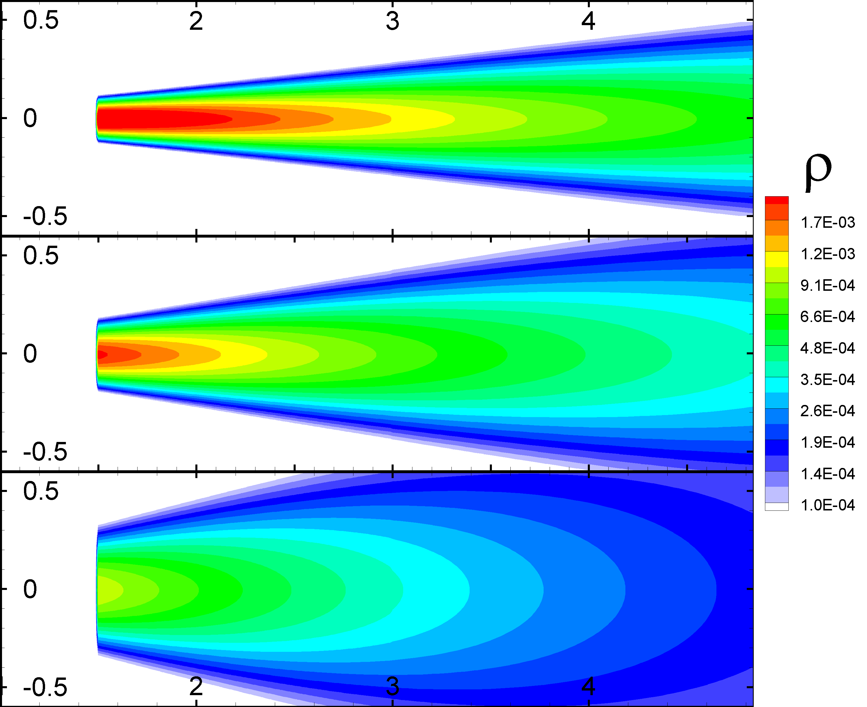
Figure 11: Discs with different aspect ratios. From top to bottom: density distribution in the $rz-$plane in three discs with differing aspect ratios of $H/r$ = 0.03, 0.05, and 0.10 but identical surface density profiles.

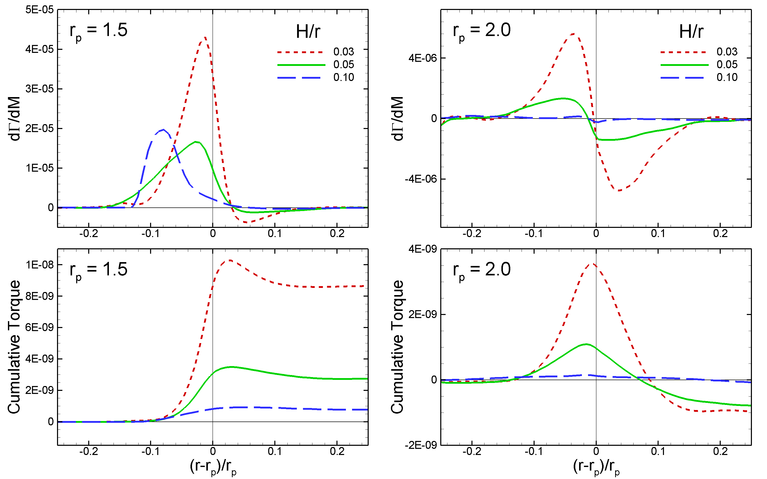
Figure 12: Torque profiles for different disc aspect ratios for a planet with mass $M_{p}=15M_{\oplus}$. Top row: the torque per unit mass as a function of normalized radius for planets starting at $r_{p}$ = 1.5 and 2.0 in three discs with differing aspect ratios, but identical surface density profiles. Bottom row: same as the top row, but showing the cumulative torque as a function of normalized radius. The profiles are time averaged over $t=70$.

In this study, we chose a relatively small initial aspect ratio, $h/r=0.03$, which corresponds to cold thin discs expected in protoplanetary systems. However, in some instances, the inner parts of the disc can be thicker due to stellar irradiation, or some other reasons. In order to investigate the effect of the disc height on planet migration, we performed calculations at larger initial disc aspect ratios: $H/r=0.05$ and $0.1$. For that, we fixed the disc’s surface density profile at $\Sigma=4\times 10^{-4}=const$ and also fixed the density (and pressure) distributions in the equatorial plane as $\rho_{eq}\sim r^{-3/2}$, $p_{eq}\sim r^{-3/2}$. Then, the fiducial densities in the discs with aspect ratios $0.05$ and $0.1$ are $\rho_{\rm d}=2.0\times 10^{-3}$ and $1.0\times 10^{-3}$, respectively. The fiducial density in the cavity is taken to be $\rho_{\rm cav}=10^{-2}\rho_{\rm d}$. Fig. 11 shows the resulting density distribution for discs with $H/r$ = 0.03, 0.05, and 0.1.

In models with larger aspect ratios, we increased the size of the simulation region in $z-$direction: in the cases of the discs with an aspect ratio of $H/r=0.05$, the region spans $z$= -1.0 to +1.0, and the number of grid cells $N_{z}=160$. In the cases of the discs with an aspect ratio of $H/r=0.1$, the region spans $z$= -2.0 to +2.0, and the number of grid cells $N_{z}=320$.

To compare the torques acting on the planets in discs with different $H/r$, we measure the torques on the planets located at $r_{p}=1.5$ (the disc-cavity boundary) and $r_{p}=2.0$ (in the disc). Fig. 12 shows the torque per unit mass (top row) and cumulative torque (bottom row) on the planet as a function of normalized radius, time averaged from $t=10-80$. Evidently, the net torque on the planet is diminished by increasing the disc’s aspect ratio for both the planet at $r_{p}=1.5$ where the corotation torque is important and at $r_{p}=2.0$ where the differential Lindblad torque dominates. The bottom panels of Fig. 12 show that the tidal torque’s dependence on the aspect ratio is nonlinear, with much stronger torques in thinner discs. This is due to the fact that as the disc thickness increases, less mass is concentrated near the disc midplane. For the corotation resonance, this means that less matter participates in the horseshoe orbit and the magnitude of the corotation torque is smaller. Similarly, for the Lindblad torques, the amplitude of the surface density perturbations raised by the planet is smaller and the torque again weakens.

The implication of these results is that for reasonable values of $H/r$, varying the disc height does not change the direction of the migration; however, it may strongly modify the migration time scale of the planet. This effect is especially significant for the planets interacting with the disc-cavity boundary where the corotation torque is important. However, since the migration direction is unaffected, the planet trapping mechanism is robust across the varying disc aspect ratios.

Appendix B Dependence on viscosity

In viscous discs, the disc matter moves inward, enters the horseshoe region and can prevent the corotation torque from saturation. To prevent saturation, the viscous time scale across the horseshoe region should be smaller than the horseshoe libration time scale (e.g. Masset 2001):

$$\frac{x_{s}^{2}}{3\nu_{\rm vis}}<\frac{4\pi r_{p}}{(3/2)\Omega_{p}x_{s}}~{}.$$ (26)

Following Masset (2001), we take the value of the half-width horseshoe region in the form of $x_{s}=0.96r_{p}\sqrt{{q_{p}}/{h}}$ and obtain the minimum value of viscosity required for saturation:

$$\nu_{\rm vis}=0.035\bigg{(}\frac{q_{p}}{h}\bigg{)}^{3/2}r_{p}^{2}\Omega_{p}~{}.$$ (27)

Taking into account that $\nu_{\rm vis}=\alpha H^{2}\Omega_{p}$, we obtain the minimum value of the $\alpha-$parameter of viscosity:

$$\alpha=0.035q^{3/2}h^{-7/2}\approx 4.3\times 10^{-4}\bigg{(}\frac{M_{p}}{5M_{\oplus}}\bigg{)}^{3/2}\bigg{(}\frac{h}{0.03}\bigg{)}^{-7/2}~{}.$$ (28)

For planets with masses $5M_{\oplus}$ and $15M_{\oplus}$, the minimum values of $\alpha$ required for the unsaturation of the corotation torque are $\alpha\approx 4.5\times 10^{-4}$ and $\alpha\approx 2.2\times 10^{-3}$, respectively.

Our main simulations were performed at zero viscosity. Here, we test the role of viscosity in our model. We switched on the module of viscosity and investigated the migration of a planet with mass $15M_{\oplus}$, located at $r_{p}=1.5$, in discs with different values of the viscosity parameter: $\alpha=10^{-5},10^{-4},10^{-3}$ and $10^{-2}$. We observed that, in all cases, the planet migrates outward (see Fig. 13). However, the migration rate is highest at the lowest values of the viscosity parameter $\alpha$. This dependence is the opposite of that expected in the cases where the viscosity is responsible for the unsaturation of the corotation torque. The reason for this dichotomy is specific to our model: the corotation torque is unsaturated due to the rapid migration of the planet from the disc-cavity boundary, while accretion due to viscosity is a slower process. In addition, in the presence of viscosity, the disc-cavity boundary becomes wider, and therefore the density gradient (and the migration rate) becomes lower. Fig. 14 shows that the density gradient does not change significantly if $\alpha\lesssim 10^{-3}$. Therefore, our quasi-steady model of the disc-cavity boundary is only applicable in the cases of low values of $\alpha$.

In the above example, a planet migrates rapidly from the region of the high density gradient. If a planet is located in the part of the disc with a lower density gradient, then the outward migration rate is lower, and the viscosity may dominate in the unsaturation of the corotation torque.

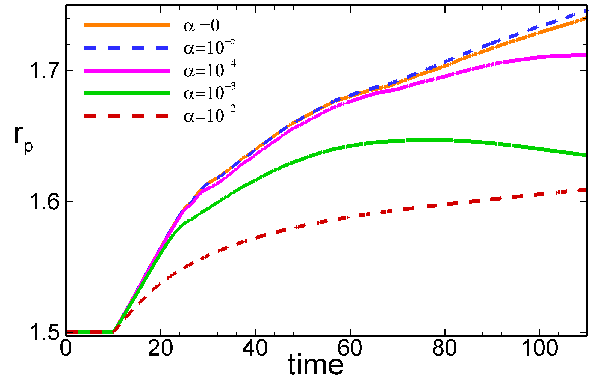
Figure 13: Variation of the planet’s semi-major axis $r_{p}$ in time in simulations with different values of viscosity parameter $\alpha$ in the disc for a planet with mass $M_{p}=15M_{\oplus}$ and initial value $r_{p}=1.5$.

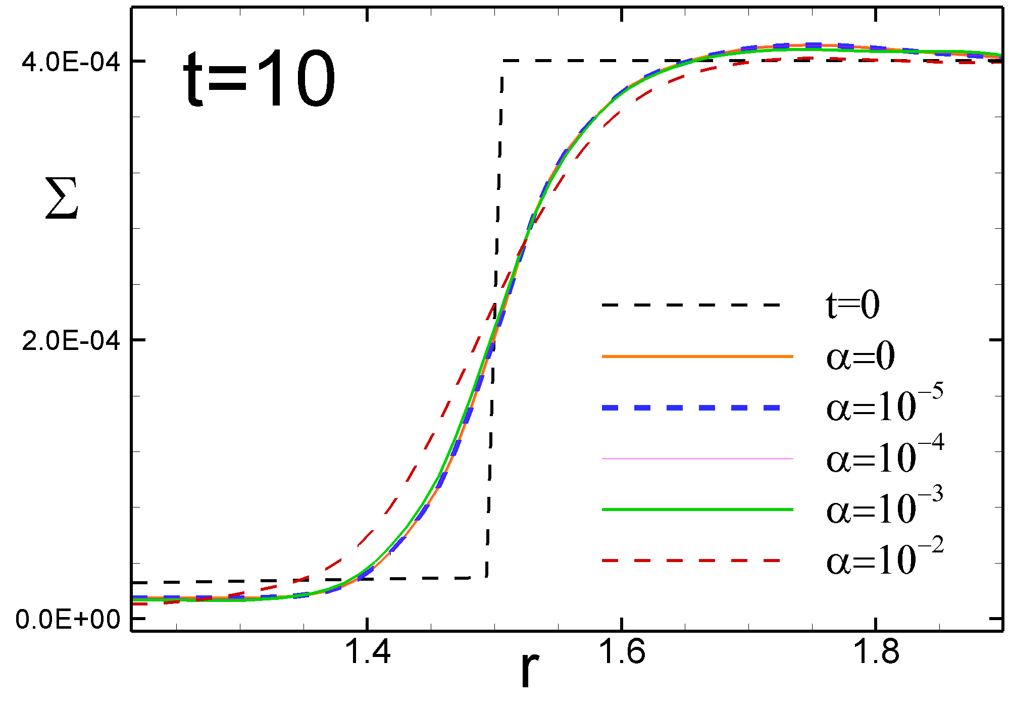
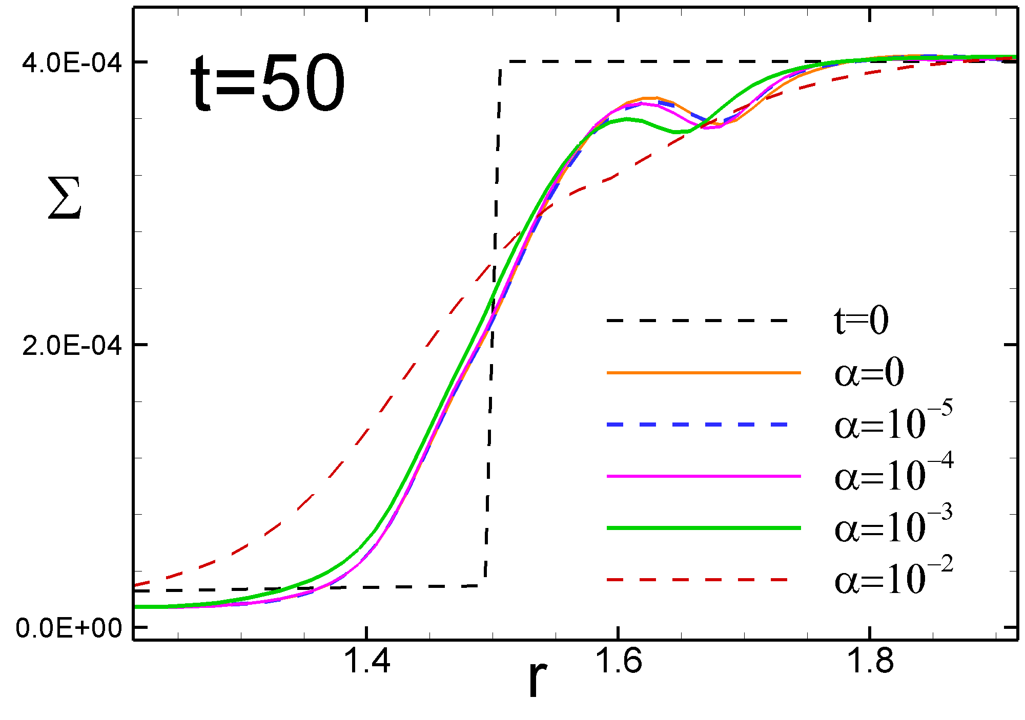
Figure 14: The surface density distribution in the vicinity of the disc-cavity boundary for three moments in time, $t=10,50,100$, for different parameters of $\alpha-$viscosity in the disc and a planet with mass $M_{p}=15M_{\oplus}$.

.

References

- Akeson et al. (2005) Akeson R. L., Walker C. H., Wood K., Eisner J. A., Scire E., Penprase B., Ciardi D. R., van Belle G. T., Whitney B., Bjorkman J. E., 2005, ApJ, 622, 440
- Artymowicz (1993a) ApJ, 419, 155
- Artymowicz (1993b) ApJ, 419, 166
- Baruteau et al. (2011) Baruteau C., Fromang, S., Nelson, R.P., Masset F., 2011, A&A, 533, A84
- Bentez-Llambay & Masset (2016) P.Bentez-Llambay, F.Masset 2016, ApJS, 223, 11
- Blinova et al. (2016) Blinova, A. A., Romanova, M. M., Lovelace, R. V. E., 2016, MNRAS, 459, 2354
- Borucki et al. (2010) Borucki, W. J., Koch, D. G., Brown, T. M., et al. 2010, ApJL, 713, L126
- Baruteau et al. (2014) Baruteau, C., Crida, A., Paardekooper, S.-J., Masset, F., Guilet, J., Bitsch, B., Nelson, R., Kley, W., Papaloizou, J. 2014, Protostars and Planets VI, Henrik Beuther, Ralf S. Klessen, Cornelis P. Dullemond, and Thomas Henning (eds.), University of Arizona Press, Tucson, 914 pp., p.667-689
- Baruteau et al. (2016) Baruteau, C., Bai, X., Mordasini, C., Molli re, P. 2016, Space Science Reviews, Volume 205, Issue 1-4, pp. 77-124
- Baruteau & Masset (2008) Baruteau C., Masset F., 2008, ApJ, 678, 483
- Brio & Wu (1988) Brio, M., & Wu, C.C., 1988, J. Comp. Phys., 75, 400
- Comins et al. (2016) Comins, M. L., Romanova, M. M., Koldoba, A. V., Ustyugova, G. V., Blinova, A. A., Lovelace, R. V. E., 2016, MNRAS, 459, 3482
- Cresswell & Nelson (2006) Cresswell P., Nelson R. P., 2006, A&A, 450, 833
- Crida et al. (2006) Crida, A., Morbidelli, A., & Masset, F. 2006, Icarus, 181, 587
- DÁngelo & Lubow (2008) DÁngelo G., Lubow S. H., 2008, ApJ, 685, 560
- DÁngelo & Lubow (2010) DÁngelo G., Lubow S. H., 2010, ApJ, 724, 730
- Donati & Landstreet (2009) Donati, J.-F., Landstreet, J. D. 2009, ARA&A, Vol. 47, 333
- Duffell (2015) Duffell, P. C., 2015, ApJ, 806, 182
- Dullemond et al. (2001) Dullemond C. P., Dominik C., Natta A., 2001, ApJ, 560, 957
- Fressin et al. (2013) Fressin, F., Torres, G., Charbonneau, D., et al., 2013, ApJ, 766, 81
- Fromang et al. (2005) Fromang S., Terquem C., Nelson R. P., 2005, MNRAS, 363, 943
- Fryxell et al. (2000) B.Fryxell et.al. 2000, ApJS, 131, 273
- Fung et al. (2015) Fung, J., Artymowicz, P., & Wu, Y., 2015, ApJ, 811, 101
- Gammie (1996) Gammie C. F., 1996, ApJ, 457, 355
- Goldreich & Tremaine (1979) Goldreich P., Tremaine S., 1979, ApJ, 233, 857
- Goldreich & Tremaine (1980) Goldreich P., Tremaine S., 1980, ApJ, 241, 425
- Guilera & Sándor (2017) Guilera, O. M., & Sándor, Zs, 2017, A&A, 604, id.A10, 18 pp.
- Hartmann (2000) Hartmann L. 2000. Accretion processes in star formation. Cambridge University Press, Vol. 32.
- Hasegawa & Pudritz (2011) Hasegawa Y., Pudritz R. E., 2011, MNRAS, 417, 1236
- Hayashi (1981) Hayashi, C. 1981, Progress of Theoretical Physics Supplement, 70, 35
- Ida & Lin (2008) Ida S., Lin D. N. C., 2008, ApJ, 685, 584
- Jiménez & Masset (2017) Jimenéz, M. A., Masset, F. S., 2017, MNRAS, 471, 4917
- Kaltenegger (2017) Kaltenegger, L., ARA&A, vol. 55, issue 1, pp. 433
- Kley (1998) Kley W. Astron. Astrophys. 1998, 338, L37
- Kley & Crida (2008) Kley W., & Crida, A. 2008, A&A, 487, L9
- Kley et al. (2009) Kley W., Bitsch B., Klahr H. 2009, A&A, 506, 971
- Kley & Nelson (2012) Kley W., Nelson R. P. 2012, ARA&A, 50, 211
- Koldoba et al. (2016) Koldoba A.V., Ustyugova G.V., Lii P.S., Comins M.L., Dyda S., Romanova M.M., Lovelace R.V.E. 2016, New Astronomy, 45, 60
- Königl (1991) Königl A., 1991, ApJ, 370, L39
- Kretke & Lin (2007) Kretke K. A., Lin D. N. C., 2007, ApJ, 664L, 55K
- Kretke & Lin (2012) Kretke K. A., Lin D. N. C., 2012, ApJ, 755, 74
- Kuchner & Lecar (2002) Kuchner M. J., Lecar M., 2002, ApJ, 574, L87
- Lee & Chiang (2017) Lee, E. J., Chiang, E. 2017, ApJ, 842, Issue 1, article id. 40, 12 pp.
- Lega et al. (2014) Lega, E.; Crida, A.; Bitsch, B.; Morbidelli, A. 2014, MNRAS, 440, 683
- Lega et al. (2015) Lega, E., Morbidelli, A., Bitsch, B., Crida, A., Szulágyi, J. 2015, MNRAS, 452, 1717
- Lin et al. (1996) Lin D. N. C., Bodenheimer P., Richardson D. C., 1996, Nature, 380, 606
- Lin & Papaloizou (1986) Lin D. N. C. & Papaloizou, J. C. B. 1986, ApJ, 309, 846
- Lin & Papaloizou (1979) Lin D. N. C. & Papaloizou, J. C. B. 1979, In: Protostars and planets III (A93-42937 17-90), p. 749
- Lin & Papaloizou (1993) Lin D. N. C. & Papaloizou, J. C. B. 1993, In: Protostars and planets III (A93-42937 17-90), p. 749
- Liu et al. (2017) Liu, B., Ormel, C.W., Lin, D. N. C. 2017, A&A, 601, A15
- Lyra et al. (2010) Lyra W., Paardekooper S.-J., Mac Low M.-M., 2010, ApJ, 715, L68
- Malik et al. (2018) Malik, M., Meru, F., L. Mayer, F. L. Meyer, M., MNRAS, submitted, arXiv:1502.06597v1
- Masset (2000) Masset F. S. 2000, A&A Supplement, 141, 165
- Masset (2001) Masset F. S. 2001, ApJ, 558, 453
- Masset (2002) Masset F. S., 2002, A&A, 387, 605
- Masset et al. (2006a) Masset F. S., Morbidelli A., Crida A., Ferreira J., 2006a, ApJ, 642, 478
- Masset et al. (2006b) Masset F. S., D’angelo, G., Kley, W., 2006b, ApJ, 652, 730
- Masset (2008) Masset F. S., 2008, EAS Publications Series, Volume 29, 2008, pp.165-244
- Masset & Casoli (2009) Masset F. S. & Casoli J. 2009, ApJ, 703, 857
- Masset & Casoli (2010) Masset F. S. & Casoli J. 2010, ApJ, 723, 1393
- Masset & Ogilvie (2004) Masset F. S. & Ogilvie G. I. 2004, ApJ, 615, 1000
- Masset & Benitéz-Llambay (2016) Masset F. S. & Benitéz-Llambay, P. 2016, ApJ, 817, Issue 1, article id. 19, 17 pp.
- Matsumura et al. (2007) Matsumura S., Pudritz R. E., Thommes E. W., 2007, ApJ, 660, 1609
- McNally et al. (2017) McNally C. P., Nelson R. P., Paardekooper S.-J., Gressel O., Lyra W., 2017, MNRAS, 472, 1565
- McNally et al. (2018) McNally C. P., Nelson R. P., Paardekooper S.-J., 2018, MNRAS, 477, 4596
- Mignone et al. (2007) Mignone A., Bodo G., Massaglia S., Matsakos T., Tesileanu O., Zanni C., Ferrari A. 2007, ApJS, 170, 228
- Mignone et al. (2012) Mignone, A., Flock, M., Stute, M., Kolb, S. M., Muscianisi, G., 2012, A&A, 545, id.A152, 16 pp.
- Miyoshi & Kusano (2005) Miyoshi, T., & Kusano, K., J. Comp. Phys., 208, 315, 2005
- Miyoshi et al. (2010) Miyoshi, T., Terada, N., Matsumoto, Y., Fukazawa, K., Umeda, T., Kusano, K., IEEE Transactions on Plasma Science, 38, 2236, 2010
- Monnier et al. (2005) Monnier J. D., Millan-Gabet R., Billmeier R., Akeson R. L., Wallace D., Berger J.-P., Calvet N., D’Alessio P., Danchi W. C., Hartmann L., Hillenbrand L. A., Kuchner M., Rajagopal J., Traub W. A., Tuthill P. G., Boden A., et al., 2005, ApJ, 624, 832
- Morbidelli et al. (2008) Morbidelli A., Crida A., Masset F., Nelson R. P., 2008, A&A, 478, 929
- Müller et al. (2012) Müller, T.W.A., Kley, W, Meru, E. 2012, A&A, 541, 13pp
- Muzerolle et al. (2003) Muzerolle J., Calvet N., Hartmann L., D’Alessio P., 2003, ApJ, 597, L149
- Nelson (2005) Nelson R. P., 2005, A&A, 443, 1067
- Nelson et al. (2000) Nelson R. P., Papaloizou J. C. B., Masset F., Kley W., 2000, MNRAS, 318, 18
- Ogilvie & Lubow (2003) Ogilvie G. I., Lubow S. H., 2003, ApJ, 587, 398
- Ogilvie & Lubow (2006) Ogilvie G. I., Lubow S. H., 2006, MNRAS, 370, 784 resonance
- Paardekooper & Mellema (2006) Paardekooper S. -J. & Mellema G. 2006, A&A, 459, L17
- Paardekooper & Mellema (2008) Paardekooper S. -J. & Mellema G. 2008, A&A, 478, 245
- Paardekooper & Papaloizou (2009a) Paardekooper S. -J., Papaloizou J. C. B., 2009, MNRAS, 394, 2283
- Paardekooper & Papaloizou (2009b) Paardekooper S. -J., Papaloizou J. C. B., 2009, MNRAS, 394, 2297
- Paardekooper & Papaloizou (2009c) Paardekooper S. -J., Papaloizou J. C. B., 2009, A&A, 485, 877
- Paardekooper et al. (2010) Paardekooper S. -J., Baruteau C., Crida A., Kley W. 2010, MNRAS, 401, 1950
- Paardekooper et al. (2011) Paardekooper S. -J., Baruteau C., Kley W. 2011, MNRAS, 410, 293
- Paardekooper (2014) Paardekooper S. -J., 2014, MNRAS, 444, 2031
- Pollack et al. (1996) Pollack, J. B., Hubickyj, O., Bodenheimer, P., Lissauer, J. J., Podolak, M., Greenzweig, Y. 1996, Icarus, 124, 62
- Qi et al. (2013) 2013, Science, 341, 630
- Rice et al. (2008) Rice W. K. M., Armitage P. J., Hogg D. F., 2008, MNRAS, 384, 1242
- Romanova et al. (2002) Romanova M. M., Ustyugova G. V., Koldoba A. V., Lovelace R. V. E, 2002, ApJ, 578, 420
- Romanova et al. (2003) Romanova M. M., Ustyugova G. V., Koldoba A. V., Wick J. V., Lovelace R. V. E, 2003, ApJ, 595, 1009
- Romanova et al. (2004) Romanova M. M., Ustyugova G. V., Koldoba A. V., Wick J. V., Lovelace R. V. E, 2004, ApJ, 610, 920
- Romanova & Lovelace (2006) Romanova M. M., Lovelace R. V. E, 2006, ApJ, 645, L73
- Shakura & Sunyaev (1973) Shakura N. I. & Sunyaev R. A. 1973, A&A, 24, 337
- Stone et al. (2008) Stone J.M., Gardiner T.S., Tauben P., Hawley J.F., Simon J.B. 2008, ApJS, 178, 137
- Tanaka et al. (2002) Tanaka H., Takeuchi T., Ward W. R. 2002, ApJ, 565, 1257
- Terquem (2003) Terquem, C.E.J.M.L.J., 2003, MNRAS, 341, 1157
- Toro et al. (1994) Toro E. F., Spruce M., Speares W., 1994, Shock Waves, 4, 25
- Uribe et al. (2011) Uribe, A. L., Klahr, H., Flock, M., Henning, Th. 2011, ApJ, 736, 85
- Ward (1986) Ward W. R., 1986, Icarus, 67, 164
- Ward (1991) Ward W. R., 1991, in: Lunar and Planetary Institute Science Conference Abstracts, vol. 22 of Lunar and Planetary Inst. Technical Report, p. 1463.
- Ward et al. (1992) Ward W. R., 1992, in Dermott S. F., Hunter Jr. J. H., Wilson R. E., eds, Astrophysical Disks Vol. 675 of Annals of the New York Academy of Sciences, p. 314
- Ward (1997) Ward W. R., 1997, Icarus, 126, 261
- Ward & Hourigan (1989) Ward, W. R., & Hourigan, K. 1989, ApJ, 347, 490
- Winn & Fabrycky (2015) Winn, J. N., & Fabrycky, D. C. 2015, ARA&A, 53, 409
- Zeng, Sasselov & Jacobsen (2016) Zeng, L., Sasselov, D. D., & Jacobsen, S. B. ApJ, 819, Issue 2, article id. 127, 5 pp.
- Zhang et al. (2007) Zhang, X., Kretke, K., Lin, D. N. C. 2007, Proceedings of IAU Symposium No. 249 Exoplanets: Detection, Formation and Dynamics, Y.-S. Sun, S. Ferraz-Mello and J.-L. Zhou, eds.