SAI
a Sensible Artificial Intelligence that plays Go

Abstract

We propose a multiple-komi modification of the AlphaGo Zero/Leela Zero paradigm. The winrate as a function of the komi is modeled with a two-parameters sigmoid function, hence the winrate for all komi values is obtained, at the price of predicting just one more variable. A second novel feature is that training is based on self-play games that occasionaly branch –with changed komi– when the position is uneven. With this setting, reinforcement learning is shown to work on 7$\times$7 Go, obtaining very strong playing agents. As a useful byproduct, the sigmoid parameters given by the network allow to estimate the score difference on the board, and to evaluate how much the game is decided. Finally, we introduce a family of agents which target winning moves with a higher score difference.

I Introduction

The longstanding challenge in artificial intelligence of playing Go at professional human level has been successfully tackled in recent works ^{1, 2, 3}, where software tools (AlphaGo, AlphaGo Zero, AlphaZero) combining neural networks and Monte Carlo tree search reached superhuman level. Such techniques can be generalised, see for instance ^{4, 5, 6}. A recent development was Leela Zero ⁷, an open source software whose neural network is trained over millions of games played in a distributed fashion, thus allowing improvements within reach of the resources of the academic community.

However, all these programs suffer from a relevant limitation: it is impossible to target their margin of victory. They are trained with a fixed initial bonus for white player (komi) of 7.5 and they are built to maximize the winning probability, without any knowledge of the game score difference.

This has several negative consequences for these programs: when they are ahead, they choose suboptimal moves, and often win by a small margin (see many of the games not ending in a resignation in ⁸); they cannot be used with komi 6.5, which is also common in professional games; they show bad play in handicap games, since the winrate is not a relevant attribute in that situations.

In principle all these problems could be overcome by replacing the binary reward (win=1, lose=0) with the game score difference, but the latter is known to be less robust ^{9, 10} and in general strongest programs use the former since the seminal works ^{11, 9, 12}.

Truly, letting the score difference be the reward for the AlphaGo Zero method, where averages of the value are computed over different positions, would lead to situations in which a low probability of winning with a huge margin could overcome a high probability of winning by 0.5 points in MCTS search, resulting in weaker play.

An improvement that would ensure the robustness of estimating winning probabilities, but at the same time would overcome these limitations, would be the ability to play with an arbitrary number of bonus points. The agent would then maximize the winning probability with a variable virtual bonus/malus, resulting in a flexible play able to adapt to positions in which it is ahead or behind taking into account implicit information about the score difference. The first attempt in this direction gave unclear results ¹³.

In this work we propose a model to pursue this strategy, and as a proof-of-concept we apply it to 7$\times$7 Go.

The source code of the SAI fork of Leela Zero and of the corresponding server can be found on GitHub at https://github.com/sai-dev/sai and https://github.com/sai-dev/sai-server.

II General ideas

II-A Winrate

The winrate $\rho$ of the current player depends on the state $s$. For the sake of generality we include a second parameter, i.e. a number $x\in\mathbb{Z}$ of virtual bonus points for the current player. So we will have $\rho=\rho(s,x)=\rho_{s}(x)$, with the latter being our standard notation. When trying to win by some amount of points $n$, the agent may let $x=-n$ to ponder its chances.

Since $\rho_{s}(x)$ as a function of $x$ must be increasing and map the real line onto $[0,1]$, a family of sigmoid functions is a natural choice:

$$\rho_{s}(x)=\sigma(x+\bar{k}_{s},\alpha_{s},\beta_{s})$$ (1)

Here we set

$$\sigma(x,\alpha,\beta):=\frac{1}{1+\exp(-\beta(\alpha+x))}$$ (2)

The number $\bar{k}_{s}$ is the signed komi, i.e. if the real komi of the game is $k$, we set $\bar{k}_{s}=k$ if at $s$ the current player is white and $\bar{k}_{s}=-k$ if it is black.

The number $\alpha=\alpha_{s}$ is a shift parameter: since $\sigma(-\alpha,\alpha,\beta)=1/2$, it represents the expected difference of points on the board from the perspective of the current player. The number $\beta=\beta_{s}$ is a scale parameter: the higher it is, the steeper is the sigmoid, generally meaning that the result is set. The highest meaningful value of $\beta$ is of the order of 10, since at the end of the game, when the score on the board is set, $\rho$ must go from about 0 to about 1 by increasing its argument by one single point. The lowest meaningful value of $\beta$ for the full 19$\times$19 board is of the order of $10/2/361\approx 0.01$, since at the start of the game, even for a very weak agent it would be impossible to lose with a 361.5 points komi in favor.

II-B Neural network: duplicate the head

AlphaGo, AlphaGo Zero, AlphaZero and Leela Zero all share the same core structure, with neural networks that for every state $s$ provide

• a probability distribution over the possible moves $p_{s}$ (the policy), trained as to choose the most promising moves for searching the tree of subsequent positions;

• a real number $v_{s}$ (the value), trained to estimate the probability of winning for the current player.

We propose a modification of Leela Zero neural network that for every state $s$ gives the usual policy $p_{s}$, and the two parameters $\alpha_{s}$ and $\beta_{s}$ described above instead of $v_{s}$.

II-C Branching from intermediate position

Training of Go neural networks with multiple komi evaluation is a challenge on its own. Supervised approach appears unfeasible, since large databases of games have typically standard komi values of 6.5, 7.5 or so and moreover it’s not possible to estimate final territory reliably for them. Unsupervised learning asks for the creation of millions of games even when the komi value is fixed. If that had to be made variable, then theoretically millions of games would be needed for each komi value.

Moreover, games started with komi very different from the natural values may well be weird, wrong and useless for training, unless one is able to provide agents with different strength. Finally, we are trying to train two parameters $\alpha_{s}$ and $\beta_{s}$ from a single output, i.e. the game outcome. To this aim, it would be advisable to have at least two finished games, with different komi, for many training states $s$.

We propose a solution to this problem, by dropping the usual choice that self-play games for training always start from the initial empty board position. The proposed procedure is the following.

1. Start a game from the empty board with random komi close to the natural one.

2. For each state in the game, take note of the estimated value of $\alpha$.

3. After the game is finished, look for states $s$ in which $d:=|\bar{k}_{s}+\alpha_{s}|$ is large: these are positions in which one of the sides was estimated to be ahead of $d$ points.

4. With some probability start a new game from states $s_{*}$ with the komi corrected by $d$ points, in such a way that the new game starts with even chances of winning, but with a komi very different from the natural one.

5. Iterate from the start.

With this approach games branch when they become uneven, generating fragments of games with natural situations in which a large komi may be given without compromising the style of game. Moreover, the starting fuseki positions, that, with the typical naive approach, are greatly over-represented in the training data, are in this way much less frequent. Finally, not all but many training states are in fact branching points for which there exists two games with different komi, yielding easier training.

II-D Agent behaviour

We incorporated in our agents the following smart choices of Leela Zero:

• the evaluation of the winrate of an intermediate state $s$ is the average of the value $v$ over the subtree of states rooted at $s$, instead of the typical minimax that is expected in these situations;

• the final selection of the move to play is done, at the root of the MCTS tree, by maximizing the number of playouts instead of the winrate.

However, we designed our agents to be able to win by large score differences. To this aim, we designed a parametric family of value functions $\nu=\nu_{\lambda}(s)$, $\lambda\in[0,1]$, as the average of $\sigma(x,\alpha,\beta)$ for $x$ ranging from $\bar{k}$ to a level of bonus/malus points $\bar{x}_{\lambda}$ that would make the game closer to be even: in other words, for $\lambda>0$, $\nu_{\lambda}(s)$ under- or over-estimates the probability of victory, according to whether the player is winning or losing.

III Proof of concept: 7$\times$7 SAI

III-A Scaling down Go complexity

Scaling the Go board from size $n$ to size $\rho n$ with $\rho<1$ yields several advantages:

• Average number of legal moves at each position scales by $\rho^{2}$.

• Average length of a game scales by $\rho^{2}$.

• The number of visits in the UC tree that would result in a similar understanding of the total game, scales at an unclear rate, nevertheless one may naively infer from the above two, that it may scale by about $\rho^{4}$.

• The number of resconv layers in the ANN tower scales by $\rho$.

• The fully connected layers in the ANN are also much smaller, even if it is more complicated to estimate the speed contribution.

All in all it is reasonable that the total speed improvement for self-play games is of the order of $\rho^{9}$ at least.

Since the expected time to train 19$\times$19 Go on reasonable hardware has been estimated to be in the order of several hundred years, we anticipated that for 7$\times$7 Go this time should be in the order of weeks. In fact, with a small cluster of 3 personal computers with average GPUs we were able to complete most runs of training in less than a week each. We always used networks with 3 residual convolutional layers of 128 filters, the other details being the same as Leela Zero. The number of visits corresponding to the standard value of 3200 used on the regular Go board would scale to about 60 for 7$\times$7. We initially experimented with 40, 100 and 250 visits and then went with the latter, which we found to be much better. The Dirichlet noise $\alpha$ parameter has to be scaled with the size of the board, according to ² and we did so, testing with the (nonscaled) values of $0.02$, $0.03$ and $0.045$. The number of games on which the training is performed was assumed to be quite smaller that the standard 250k window used at size 19, and after some experimenting we observed that values between 8k and 60k generally give good results.

III-B Neural network structure

As explained in Section II-B, Leela Zero’s neural network provides for each position two outputs: policy and winrate. SAI’s neural network should provide for each position three outputs: the policy as before and the two parameters $\alpha$ and $\beta$ of a sigmoid function which would allow to estimate the winrate for different komi values with a single computation of the net. It is unclear whether the komi itself should be provided as an input of the neural network: it may help the policy adapt to the situation, but could also make the other two parameters unreliable. For the initial experiments the komi will not be provided as an input to the net.

With the above premises, the first structure we propose for the network is very similar to Leela Zero’s one, with the value head substituted by two identical copies of itself devoted to the parameters $\alpha$ and $\beta^{*}$. The latter is then mapped to $\beta$ by equation $\beta_{s}=c\exp(\beta^{*}_{s})$. The exponential transform imposes the natural condition that $\beta$ is always positive. The constant $c$ is clearly redundant when the net is fully trained, but the first numerical experiments show that it may be useful to tune the training process at the very beginning, when the net weights are almost random, because otherwise $\beta$ would be close to 1, which is much too large for random play, yielding training problems. The two outputs were trained with the usual $l^{2}$ loss function but with the value $v_{s}$ substituted with $\rho_{s}(0)=\sigma(\bar{k}_{s},\alpha_{s},\beta_{s})$.

We used two structures of network, type V and type Y, which are described in detail in ¹⁴.

III-C Branching from intermediate positions

To train the network we included the komi value into the training data used by SAI. The training is then performed the same way as for Leela Zero, with the loss function given by the sum of regularization term, cross entropy for the policy and $l^{2}$ norm for the winning rate.

The winning rate is computed with the sigmoid function given by equations (1) and (2), in particular we set $v(s)=\rho_{s}(0)$ and backpropagate gradients through these functions.

To train the neural network it is clearly necessary to have different komi values in the data set. It would be best to have very different komi values, but when the agent starts playing well enough, only few values around the correct komi make the games meaningful.

To adapt the komi values range to the ability of the current network, when the server assign a self-play match to a client, it chooses a komi value randomly generated with distribution given by the sigmoid itself. Formally,

$$K=0.5+\lfloor\rho_{s}^{-1}(U)\rfloor$$ (3)

where $\rho_{s}(x)=\sigma(x,\alpha_{s},\beta_{s})$, $s$ is the initial empty board state, $\alpha_{s}$ and $\beta_{s}$ are the computed values with current network and $U\sim\operatorname{unif}(0,1)$, thus giving to $K$ an approximate logistic distribution.

As the learning goes on, we expect $\alpha_{s}$ to converge to the correct value of 9, and $\beta_{s}$ to increase, narrowing the range of generated komi values.

To deal with this problem we implemented the possibility for the server to assign self-play games starting from any intermediate position.

After a standard game is finished, the server looks to each of the game’s positions and from each one may branch a new game (independently and with small probability). The branched game starts at that position with a komi value that is considered even by the network. Formally,

$$k^{\prime}=0.5+\lfloor\pm\alpha_{s}\rfloor$$

where $s$ is the branching position and $\pm\alpha_{s}$ is the value of $\alpha$ at position $s$, as computed by the current network, with the sign changed if the current player was white.

The branched game is then played until it finishes and then all its positions starting from $s$ are stored in the training data, with komi $k^{\prime}$ and the correct information on the winner of the branch.

This procedure should produce branches of positions with unbalanced situations and values for the komi that are natural to the situation but nevertheless range on a wide interval of values.

III-D Sensible agent

When SAI plays, it can estimate the winrate for all values of the komi with a single computation of the neural network. In fact, getting $\alpha$ and $\beta$ it knows the sigmoid function that gives the probability of winning with different values of the komi for the current position.

We propose the generalization of the original agent of Leela Zero as introduced in Section II-D. Here we give further details.

The agent behaviour is parametrized by a real number $\lambda$ which will be usually chosen in $[0,1]$.

To describe rigorously the agent, we need to introduce some more mathematical notation.

Games, moves, trees.

Let $\mathcal{G}$ be the set of all legal game states, with $\varnothing\in\mathcal{G}$ denoting the empty board starting state.

For every $s\in\mathcal{G}$, let $\mathcal{A}_{s}$ the set of legal moves at state $s$ and for every $a\in\mathcal{A}_{s}$, let $s_{a}\in\mathcal{G}$ denote the game state reached from $s$ by performing move $a$. This clearly induces a directed graph structure on $\mathcal{G}$ with no directed cycles (which are not legal because of superko rule) and with root $\varnothing$. This graph can be uplifted to a rooted tree by taking multiple copies of the states which can be reached from the root by more than one path. From now on we will identify $\mathcal{G}$ with this rooted tree and denote by $\rightarrow$ the edge relation going away from the root.

For all $s\neq\varnothing$ let $\bar{s}$ denote the unique state such that $\bar{s}\rightarrow s$.

For all $s\in\mathcal{G}$, let $\mathcal{R}_{s}=\{r\in\mathcal{G}:s\rightarrow r\}$ denote the set of states reachable from $s$ by a single move. We will identify $\mathcal{A}_{s}$ with $\mathcal{R}_{s}$ from now on.

For any subtree $T\subset\mathcal{G}$, let $|T|$ denote its size (number of nodes) and for all $s\in T$, let $T_{s}$ denote the subtree of $T$ rooted at $s$.

Values, preferences and playouts.

Suppose that we are given three maps $P$, $u$ and $v$, with the properties described below.

• The policy $P$, defined on $\mathcal{G}$ with values in $[0,1]$ and such that

  $$\sum_{r\in\mathcal{R}_{s}}P(r)=1,\qquad s\in\mathcal{G}.$$

  This map represents a measure of goodness of the possible moves.

• The value $v$, defined on $\{(s,r):s\in\mathcal{G},r\in\mathcal{G}_{s}\}$ with values in $[0,1]$, which represents a rough estimate of the winrate at a future state $r$. The estimate is from the point of view of whichever player is next to play at state $s$.

• The first play urgency $u$, defined for all pairs $(s,T)$ such that $s\in\mathcal{G}$ and $T\subset\mathcal{G}$ with values in $[0,1]$. This represents an “uninformed”, flat, winning rate estimate of all states in $\mathcal{R}_{s}\setminus T$, i.e. actions which were not yet visited. It may depend on the set $T$ of visited states.

Then for any non-empty subtree $T$ and node $s$ not necessarily inside $T$ we can define the evaluation of $s$ over $T$, as

$$Q_{T}(s):=\begin{cases}u(\bar{s},T)&\text{if }s\notin T\\[4.30554pt] \displaystyle\frac{1}{|T_{s}|}\sum_{r\in T_{s}}v(\bar{s},r)&\text{if }s\in T\end{cases}$$

It should be noted here that the two proposed choices for $u$ are the following:

$$u(s,T)\equiv 0.5$$ (AlphaGo Zero)

$$u(s,T)=v(s,s)-C_{\text{fpu}}\sqrt{\sum_{r\in\mathcal{R}_{s}\cap T}P(r)}$$ (Leela Zero)

We can then define the UC urgency of $s$ over $T$, as

$$U_{T}(s):=Q_{T}(s)+C_{\text{puct}}\sqrt{|T_{\bar{s}}|-1}\frac{P(s)}{1+|T_{s}|}$$

Finally, the playout over $T$, starting from $s\in T$ is defined as the unique path on the tree which starts from $s$ and at every node $r$ chooses the node $t\in\mathcal{R}_{r}$ that maximizes $U_{T}(t)$.

Definition of $v$.

In the case of Leela Zero, the value function $v(s,r)$ depends on $s$ only through parity: let $\hat{v}_{r}$ be the estimate of the winning rate of current player at $r$, i.e. the output of the value head of the neural network, passed through an hyperbolic tangent and rescaled in $(0,1)$. Then

$$v(s,r):=\begin{cases}\hat{v}_{r}&s,r\text{ with same current player}\\ 1-\hat{v}_{r}&s,r\text{ with different current player}\end{cases}$$

In the case of SAI, the neural network provides the sigmoid’s parameters estimates $\hat{\alpha}_{r}$ and $\hat{\beta}_{r}$ for the state $r$. These allow to compute the estimate $\hat{\rho}_{r}$ of the winning probability for the current player at all komi values.

$$\hat{\rho}_{r}(x):=\sigma(\hat{\beta}_{r}(\hat{\alpha}_{r}+\bar{k}_{r}+x))$$

Here $\bar{k}_{r}$ is the official komi value from the perspective of the current player, at state $r$,

$$\bar{k}_{s}:=\begin{cases}k&\text{if at $s$ the current player is white}\\ -k&\text{if at $s$ the current player is black},\end{cases}$$

the komi correction $x$ is a real variable that allows to fake an arbitrary virtual komi value, and $\sigma$ is the standard logistic sigmoid,

$$\sigma(x):=\frac{1}{1+e^{-x}}=\frac{1}{2}+\frac{1}{2}\tanh\biggl{(}\frac{x}{2}\biggr{)}.$$

Then if we want SAI to simulate the playing style of Leela Zero, though with its own understanding of the game situations, we can simply let

$$v(s,r):=\begin{cases}\hat{\rho}_{r}(0)&s,r\text{ with same current player}\\ 1-\hat{\rho}_{r}(0)&s,r\text{ with different current player.}\end{cases}$$

On the other hand, if we want SAI to play “sensibly”, we may use values of $x$ for which $\hat{\rho}_{r}(x)$ is away from 0 and from 1, so that it can better distinguish the consequences of its choices, as they reflect more in the winrate. This means to give the agent a positive virtual komi correction if it is behind and a negative virtual komi correction if it is ahead.

One way this can be done in a robust way, is to compute the average of the expected winrate at the future state $r$ over a range of komi correction values that depends on the current state $s$: an interval of positive numbers if the net believes that $s$ is losing and negative if winning.

By deciding the interval at $s$, we are avoiding situations like when the current player is winning at $s$, it explores a sequence of future moves with a blunder, so that it is losing at $r$, and then evaluates the winrate at $r$ giving itself a bonus which will then mitigate the penalization.

In fact, in this way blunders done when ahead are penalized more than before in the exploration, which seems a good feature.

Formally, we introduce the symbol $\mu_{r}(y)$ to denote the average of $\hat{\rho}_{r}$ over the interval $[0,y]$ or $[y,0]$,

$$\mu_{r}(y):=\begin{cases}\hat{\rho}_{r}(0)&y=0\\[4.30554pt] \displaystyle\frac{1}{y}\int_{0}^{y}\hat{\rho}_{r}(x)dx&y\neq 0.\end{cases}$$ (4)

Let the common sense parameter $\lambda$ be a real parameter, usually in $[0,1]$, and let $\pi_{\lambda}$ be

$$\pi_{\lambda}:=(1-\lambda)\hat{\rho}_{s}(0)+\lambda\frac{1}{2}$$

so that $\pi_{0}=\hat{\rho}_{s}(0)$, $\pi_{1}=\frac{1}{2}$ and $\pi_{\lambda}$ a convex combination of the two for $\lambda\in[0,1]$. We introduce the extremum of the komi correction interval as the reverse image of $\pi_{\lambda}$,

$$\bar{x}_{s,\lambda}:=\hat{\rho}_{s}^{-1}(\pi_{\lambda})$$

Then for a version of SAI which plays with parameter $\lambda$, we let the value be defined by,

$$v(s,r):=\begin{cases}\mu_{r}(\bar{x}_{s,\lambda})&s,r\text{ with same current player}\\ 1-\mu_{r}(\bar{x}_{s,\lambda})&s,r\text{ with different current player.}\end{cases}$$

Hence the value is computed at state $r$ but the range of the average is decided at state $s$.

Remark 1.

We bring to the attention of the reader that a simple rescaling shows that the quantity $\mu_{r}(\bar{x}_{r,\lambda})$ would be somewhat less useful, because it depends on $\hat{\alpha}_{r}$ and $\hat{\beta}_{r}$ only through $\hat{\rho}_{r}(0)$.

Remark 2.

As shown in ¹⁴, the integral in equation (4) can be computed analytically and easily implemented in the software.

$$\mu_{r}(y)=\frac{1}{2}+\frac{b-a}{2y}-\frac{1}{\hat{\beta}_{r}y}\log\sigma\bigl{(}\hat{\beta}_{r}b\bigr{)}+\frac{1}{\hat{\beta}_{r}y}\log\sigma\bigl{(}\hat{\beta}_{r}a\bigr{)}$$

where $a:=|\hat{\alpha}_{r}+\bar{k}_{r}|$ and $b:=|\hat{\alpha}_{r}+\bar{k}_{r}+y|$.

Tree construction and move choice.

Suppose we are at state $t\in\mathcal{G}$ and the agent has to choose a move in $\mathcal{A}_{t}$. This will be done by defining a suitable decision subtree $\mathcal{T}$ of $\mathcal{G}$, rooted at $t$, and then choosing the move $s$ randomly inside $\mathcal{R}_{t}$ with probabilities proportional to

$$\exp(C_{\text{temp}}^{-1}|\mathcal{T}_{s}|),\qquad s\in\mathcal{R}_{t}$$

where $C_{\text{temp}}$ is the Gibbs temperature which is defaulted to 1 for the first moves of self-play games and to 0 (meaning that the move with highest $|\mathcal{T}_{s}|$ is chosen) for other moves and for match games.

The decision tree $\mathcal{T}$ is defined by an iterative procedure. In fact we define a sequence of trees $\{t\}=:T^{(1)}\subset T^{(2)}\subset\dots$ and stop the procedure by letting $\mathcal{T}:=T^{(N)}$ for some $N$ (usually the number of visits or when the thinking time is up).

The trees in the sequence are all rooted at $t$ and satisfy $|T^{(n)}|=n$ for all $n$, so each one adds just one node to the previous one:

$$T^{(n)}=T^{(n-1)}\cup\{t_{n}\}$$

The new node $t_{n}$ is defined as the first node outside $T^{(n-1)}$ reached by the playout over $T^{(n-1)}$ starting from $s$.

III-E Measuring playing strength

To provide a benchmark for the developement of SAI, we adapted Leela Zero to 7$\times$7 Go board and performed several runs of training from purely random play to a level at which further improvement wasn’t expected. More details on this step can be found in ¹⁴. A sample of 7$\times$7 Leela Zero nets formed the panel used in the evaluation phase of the SAI runs.

When doing experiments with training runs of Leela Zero, we produce many networks, which had to be tested to measure their playing strength, so that we can assess the performance and efficiency of each run.

The simple usual way to do so is to estimate an Elo/GOR score for each network. The idea which defines this number is that if $s_{1}$ and $s_{2}$ are the scores of two nets, then the probability that the first one wins against the second one in a single match is

$$\frac{1}{1+e^{(s_{2}-s_{1})/c}}$$

so that $s_{1}-s_{2}$ is, apart from a scaling coefficient $c$ (traditionally set to 400), the log-odds-ratio of winning.

This model is so simple that is actually unsuitable to deal with the complexity of Go and Go playing ability. In fact in several runs of Leela Zero 7$\times$7 we observed that each training phase would produce at least one network which solidly won over the previous best, and was thus promoted to new best. This process would continue forever, or at least as long as we dared keep the run going, even if from some point on, the observed playing style was not evolving anymore. When some match was tried between non-consecutive networks, we saw that the strength inequality was not transitive, in that it was easy to find cycles of 3 or more networks that regularly beat each other in a directed circle. Even with very strong margins.

We even tried to measure the playing strength in a more refined way, by performing round-robin tournaments between nets and then estimating Elo score by maximum likelihood methods. This is much heavier to perform and still showed poor improvement in predicting match outcomes.

It must be noted that this appears to be an interesting research problem in its own. The availability of many artificial playing agents with different styles, strengths and weaknesses will open new possibilities in collecting data and experimenting in this field.

Remark 3.

It appears that this problem is mainly due to the peculiarity of 7$\times$7 Go and only relevant to it.

In the official 19$\times$19 Leela Zero project the Elo estimation is done with respect to previous best agent only and it is known that there is some Elo inflation, but tests against a fixed set of other opponents or against further past networks have shown that real playing strength does improve.

A different approach which is both robust and refined and is easy to generalize is to use a panel of networks to evaluate the strength of each new candidate.

We chose 15 networks of different strength from the first 5 runs of Leela Zero 7$\times$7. Each network to be evaluated is opposed to each of these in a 100 games match. The result is then a vector of 15 sample winning rates, which contains useful multivariate information on the playing style, strengths and weaknesses of the tested net.

To summarize this information in one rough scalar score number, we used principal component analysis (PCA). We performed covariance PCA once for all the match results of the first few hundreds of good networks, determined the principal factor and used its components as weights. Hence the score of a network is the principal component of its PCA decomposition. This value, which we call panel evaluation, correlates well with the maximum likelihood estimation of Elo by round-robin matches, but is much easier and quicker to compute.

IV Results

IV-1 Obtaining a strong SAI

	Network		Parameters during self-play					Results
Run	Type	IP	MV	FPU	ST	RT	$\lambda$	PE	TTP
SAI 9	V	18	250	AGZ	1.0	1.0	0.5	2.34848	1838
SAI 15	Y	18	250	AGZ	2.0	0.5	0.0	1.94057	1194
SAI 20	Y	17	250	LZ	1.5	0.8	0.5	2.38155	463
SAI 22	Y	17	502	LZ	1.5	0.8	0.5	2.39176	2545
SAI 23	Y	17	250	LZ	1.0	1.0	0.5	2.35204	465
SAI 24	Y	17	250	LZ	1.0	1.0	0.0	2.38220	528

TABLE I: Description of a representative sample of SAI runs. Type: shape of the network. IP: number of input planes. MV: max visits. FPU: first playing urgency, with values AGZ (AlphaGo Zero) and LZ (Leela Zero). ST: softmax temperature. RT: random temperature. $\lambda$: parameter of the agent. PE: panel evaluation of the 3rd best net of the run. TTP: time to plateau, in millions of nodes.

The first runs of SAI failed to reach the performance of the reference $7\times 7$ Leela Zero runs. A turning point was the 9th run, when we simplified the formula for the branching probability and assigned constant probability of branching $C_{\text{branch}}=0.025$ for all states, thus giving higher chance of branching in balanced situation. This resulted in a steady and important improvement. In Table I we summarized the characteristics of the most representative runs we ran after the 9th, together with their performance, measured as the panel evaluation of the 3rd best net of the run, and efficiency, measured in terms of time to reach the plateau level. In Figure 1 we represented the evolution of the performance of the same runs, across millions of nodes. Run 15 was the lowest point, showing that increasing the softmax temperature too much, while decreasing the random temperature, produced negative results. After run 15th we also settled for the Leela Zero form of first playing urgency, as opposed to AlphaGo Zero’s. Run 20th had the best balance between performance and efficiency. Increasing the maximum number of visits in run 22nd resulted in a severe loss of efficiency, not adequately compensated by a gain in performance. In runs 23rd and 24th the two temperature parameters were slightly modified again, and $\lambda$ was set to 0 and 0.5 respectively, without significant gains.

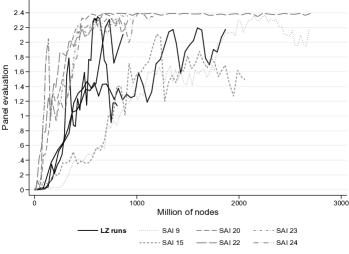
Figure 1: Panel evaluation, as a function of the millions nodes computed. Best three runs of Leela Zero reported as a landmark.

IV-2 Evaluation of positions by Leela Zero and by SAI

To illustrate the ability of SAI to understand the winrate in a more complex fashion, we chose 5 meaningful positions which are shown in Figure 2. The first 3 positions were chosen from a sample of games as the most frequent which offered two different winning moves, one with higher score than the other. The 4th and 5th positions were created ad hoc as positions where the victory is granted for the current player, but two different moves give a different score.

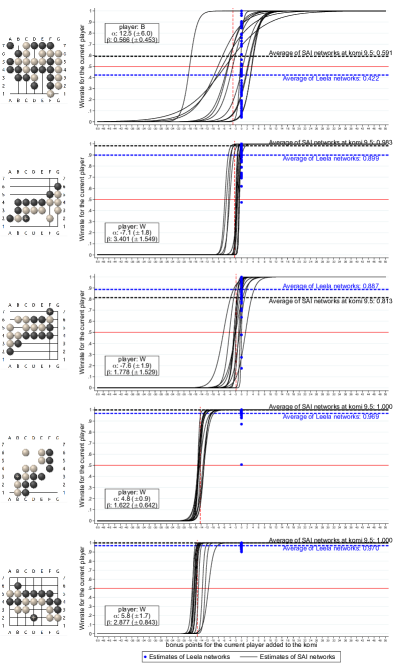
Figure 2: Evaluation of five positions by a sample of strong $7\times 7$ Leela Zero and SAI nets.

For each position we plotted SAI’s sigmoid evaluations of the winrate (black curves) and $7\times 7$ Leela Zero’s point estimates of winrate at standard komi (blue dots). Every one of these plots shows a sample of 63 $7\times 7$ Leela Zero and 13 SAI nets from different runs, chosen among the strongest ones.

It is important to observe that the distributions of the winrates seem to agree for the two groups at standard komi, indicating that SAI’s estimates have similar accuracy and precision as $7\times 7$ Leela Zero’s.

The SAI nets provide an estimate of the difference of points between the players. The variability that we observe shows that even strong nets do not have a uniform understanding of single complicated positions. However we can observe that the wider the discrepancies among estimates of $\alpha$, the lower the estimate of $\beta$, thus showing that the nets are aware that the estimate is unstable. This confirms the robustness of our approach.

We analyse separately each position, using human expertise.
Position 1. Black, the current player, is ahead of 13 points on the board, thus, with komi 9.5, his margin is 3.5 points. However the position is difficult, because there is a seki: this is a situation when an area of the board provides points (is alive) for both players (quite uncommon in our 7$\times$7 games), and may be poorly interpreted as white dead (black ahead by 49 points on the board) or as black dead (black ahead by 5 points on the board). In agreement with this analysis, the sample of SAI nets gives a low and sharp estimate for $\beta$ with average $0.566$ and standard deviation $0.453$ and a wild estimate for $\alpha$, with average $12.5$ and standard deviation $6.0$. The sample of Leela Zero nets gives winrate estimates which are almost uniformly distributed in $[0,1]$: many of these nets have an incorrect understanding of the position and are not aware of this. SAI nets on the other hand are aware of the high level of uncertainty.
Position 2. White, the current player, is behind by 5 points on the board, thus, with komi 9.5, she is winning by 4.5 points. Following the policy, which recognizes a common shape here, many nets will consider cutting at F6 instead of E5, therefore losing one point. Accordingly, the estimate of $\alpha$ ranges approximately from $-5.5$ to $-8.5$ with average $-7.1$ and standard deviation $1.8$. The sample of $\beta$ has average $3.401$ and standard deviation $1.549$, thus showing that $\alpha$ is to be considered precise up to two units.
Position 3. Here the situation is very similar to the previous one: white is behind by 7 points on the board, thus, with komi 9.5, white is winning by 2.5 points. Following the policy, which recognizes a common shape here, many nets will consider cutting at B2 instead than C3, therefore losing one point. Accordingly, the estimate of $\alpha$ ranges approximately from $-5.5$ to $-9.5$ with average $-7.6$ and standard deviation $1.9$. The sample of $\beta$ has average $1.778$ and standard deviation $1.529$, thus showing that $\alpha$ is to be considered precise up to two units.
Position 4. White, the current player, is ahead by 5 points on the board, thus, with komi she is winning by a larger margin of 14.5 points. Following the policy, white is facing the choice between B4 and A3, capturing the single black stone. There is a slight strategic difference between B4 and A3: A3 is better in case a ko fight emerges. Accordingly, we found a sharp estimate for $\alpha$ ranging from 4 to $5.5$, with average $4.8$ and standard deviation $0.8$. The sample of $\beta$ has average $1.622$ and standard deviation $0.642$.
Position 5. White, the current player, is ahead by 5 points on the board, thus, with komi, she is winning by a larger margin of $14.5$ points. The position is particularly easy to understand: white will win with every possible move on the board, including the pass; although only the move A3 gives white the largest possible victory. Accordingly, the estimate of $\alpha$ range from 4 to $7.5$ with average $5.8$ and standard deviation $1.7$. The sample of $\beta$ has average $2.877$ and standard deviation $0.843$.

IV-3 Experimenting different agents for SAI

Finally, we experimented on how the parameter $\lambda$ of the agent affects the preference of the next move, from positions where at least two winning moves are available. This was done using the 5 positions shown in Figure 2 and asking to the same 13 SAI nets to choose the next move. The parameter $\lambda$ was set to 0, 0.5 and 1, 1000 times each. In Figure 3 the results are represented. In position 1 and 5 the optimal move was chosen more than 90% of times for $\lambda=0$ already, and incresing $\lambda$ did not affet the choice. In the other 3 positions increasing $\lambda$ improved the choice of the optimal move, as expected.

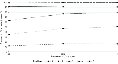
Figure 3: Probability that a net chooses the optimal move from each of the five positions, for increasing values of the $\lambda$ parameter.

V Conclusions

We introduced SAI, a reinforcement learning solution for playing Go which generalizes the previous models to multiple komi. The winrate as function of komi is estimated by a two-parameters family of sigmoid curves. We performed several complete training runs on the simplified 7$\times$7 goban, exploring parameters and settings, and proving that it is more difficult, but possible, to effectively train the net to learn two continuous parameters in spite of the fact that the match outcome is a single binary value (win/lose). The generation of a suitable ensemble of game branches with adjusted komi appears to be a key point to this end.

The estimates of the winrate of our nets at standard komi are compatible with those of Leela Zero, but at the same time SAI’s winrate curves provide a deeper understanding of the game situation. As a side effect, a good estimate of the final point difference between players can also be deduced from the winrate curves.

In principle the winrate curve estimation allows to design sensible agents that aim to win by larger margins of points against weaker opponents, or that can play with handicap in points and/or stones. We propose such an agent, parametrized by a common sense parameter $\lambda\geq 0$. When $\lambda=0$ the agent behaves like previous models and only tries to win. (We could obtain nets able to play at almost perfect level at $\lambda=0$.)

With $\lambda>0$ the agent is designed to try to win by a high margin of points, while still focusing on winning. Due to the limitations of the 7$\times$7 goban, it was not possible to assess whether our model could really target higher margins of victory against weak opponents, but we showed the expected effect of different values of $\lambda$ on the move selection.

We posit that it should be feasible to implement SAI in the 9$\times$9 and full 19$\times$19 board. Albeit the configuration of the learning pipeline presents more difficulties than standard Leela Zero and the training could be longer, the experiments performed on the 7$\times$7 board should be useful to make the right choices and develop some understanding of the possible unwanted behaviours in order to avoid them.

The development of a 19$\times$19 board version of SAI with a distributed effort could produce a software tool able to provide a deeper understanding of the potential of each position, to target high margins of victory and play with handicap, thus providing an opponent for human players which never plays sub-optimal moves, and ultimately progressing towards the optimal game.

References

- Silver et al. [2016] D. Silver et al., “Mastering the game of Go with deep neural networks and tree search,” Nature, vol. 529, no. 7587, pp. 484–489, 2016.
- Silver et al. [2018] ——, “A general reinforcement learning algorithm that masters chess, shogi, and Go through self-play,” Science, vol. 362, no. 6419, pp. 1140–1144, 2018.
- Silver et al. [2017] ——, “Mastering the game of Go without human knowledge,” Nature, vol. 550, no. 7676, pp. 354–359, 2017.
- Wang and Sun [2018] K. Wang and W. Sun, “Meta-modeling game for deriving theoretical-consistent, micro-structural-based traction-separation laws via deep reinforcement learning,” 2018. [Online]. Available: \urlhttp://arxiv.org/abs/1810.10535
- Shao et al. [2018] Y. Shao, S. C. Liew, and T. Wang, “Alphaseq: Sequence discovery with deep reinforcement learning,” 2018. [Online]. Available: \urlhttp://arxiv.org/abs/1810.01218
- Pathak and Kapila [2018] K. Pathak and J. Kapila, “Reinforcement evolutionary learning method for self-learning,” 2018. [Online]. Available: \urlhttp://arxiv.org/abs/1810.03198
- Gian-Carlo Pascutto and contributors [2018] Gian-Carlo Pascutto and contributors, “Leela Zero,” 2018, [Accessed 17-August-2018]. [Online]. Available: \urlhttp://zero.sjeng.org/home
- Törmänen [2017] A. Törmänen, Invisible: the games of AlphaGo. Hebsacker Verlag, 2017.
- Gelly et al. [2006] S. Gelly et al., “Modification of UCT with Patterns in Monte-Carlo Go,” INRIA, Research Report RR-6062, 2006. [Online]. Available: \urlhttps://hal.inria.fr/inria-00117266v3
- Silver et al. [2007] D. Silver, R. Sutton, and M. Müller, “Reinforcement Learning of Local Shape in the Game of Go,” in IJCAI, vol. 7, 2007, pp. 1053–1058.
- Coulom [2006] R. Coulom, “Efficient selectivity and backup operators in Monte-Carlo tree search,” in CG, 2006, pp. 72–83.
- Gelly and Silver [2007] S. Gelly and D. Silver, “Combining online and offline knowledge in UCT,” in ICML, 2007, pp. 273–280.
- Wu et al. [2017] T. Wu et al., “Multi-Labelled Value Networks for Computer Go,” 2017. [Online]. Available: \urlhttp://arxiv.org/abs/1705.10701
- Morandin et al. [2018, version 1] F. Morandin et al., “SAI, a Sensible Artificial Intelligence that plays Go,” 2018, version 1. [Online]. Available: \urlhttps://arxiv.org/abs/1809.03928v1