Hydrograph peak-shaving using a graph-theoretic algorithm for placement of hydraulic control structures

Abstract

The need to attenuate hydrograph peaks is central to the design of stormwater and flood control systems. However, few guidelines exist for siting hydraulic control structures such that system-scale benefits are maximized. This study presents a graph-theoretic algorithm for stabilizing the hydrologic response of watersheds by placing controllers at strategic locations in the drainage network. This algorithm identifies subcatchments that dominate the peak of the hydrograph, and then finds the “cuts” in the drainage network that maximally isolate these subcatchments, thereby flattening the hydrologic response. Evaluating the performance of the algorithm through an ensemble of hydrodynamic simulations, we find that our controller placement algorithm produces consistently flatter discharges than randomized controller configurations—both in terms of the peak discharge and the overall variance of the hydrograph. By attenuating flashy flows, our algorithm provides a powerful methodology for mitigating flash floods, reducing erosion, and protecting aquatic ecosystems. More broadly, we show that controller placement exerts an important influence on the hydrologic response and demonstrate that analysis of drainage network structure can inform more effective stormwater control policies.

Highlights

• New algorithm for placing hydraulic control structures in drainage networks.

• Attenuates downstream hydrograph by de-synchronizing tributary flows.

• Algorithm is fast and requires only digital elevation data.

1 Introduction

In the wake of rapid urbanization, aging infrastructure and a changing climate, effective stormwater management poses a major challenge for cities worldwide [1]. Flash floods are one of the largest causes of natural disaster deaths in the developed world [2], and often occur when stormwater systems fail to convey runoff from urban areas [3]. At the same time, many cities suffer from impaired water quality due to inadequate stormwater control [4]. Flashy flows erode streambeds, release sediment-bound pollutants, and damage aquatic habitats [4, 5, 6, 7], while untreated runoff may trigger fish kills and toxic algal blooms [8, 9]. Engineers have historically responded to these problems by expanding and upsizing stormwater control infrastructure [10]. However, larger infrastructure frequently brings adverse side-effects, such as dam-induced disruption of riparian ecosystems [11], and erosive discharges due to overdesigned conveyance infrastructure [1]. As a result, recent work has called for the replacement of traditional peak attenuation infrastructure with targeted solutions that better reduce environmental impacts [12, 13].

As the drawbacks of oversized stormwater infrastructure become more apparent, many cities are turning towards decentralized stormwater solutions to regulate and treat urban runoff while reducing adverse impacts. Green infrastructure, for instance, uses low-impact rain gardens, bioswales, and green roofs to condition flashy flows and remove contaminants [14, 15, 16]. Smart stormwater systems take this idea further by retrofitting static infrastructure with dynamically controlled valves, gates and pumps [1, 17, 18, 19]. By actuating small, distributed storage basins and conveyance structures in real-time, smart stormwater systems can halt combined sewer overflows [20], mitigate flooding [1], and improve water quality at a fraction of the cost of new construction [1, 17]. While decentralized stormwater management tools show promise towards mitigating urban water problems, it is currently unclear how these systems can be designed to achieve maximal benefits at the watershed scale. Indeed, some research suggests when stormwater control facilities are not designed in a global context, local best management practices can lead to adverse system-scale outcomes—in some cases inducing downstream flows that are more intense than those produced under unregulated conditions [21, 22].

Thus, as cities begin to experiment with decentralized stormwater control, the question of where to place control structures becomes crucial. While many studies have investigated the ways in which active control can realize system-scale benefits (using techniques like feedback control [23], market-based control [20], or model-predictive control, [24, 25]), the location of control structures within the drainage network may serve an equally important function. Hydrologists have long recognized the role that drainage network topology plays in shaping hydrologic response [26, 27, 28, 29, 30, 31, 32, 33, 34]. It follows that strategic placement of hydraulic control structures can shape the hydrograph to fulfill operational objectives, such as maximally flattening flood waves and regulating erosion downstream. To date, however, little research has been done to assess the problem of optimal placement of hydraulic control structures in drainage networks:

• Recent studies have investigated optimal placement of green infrastructure upgrades like green roofs, rain tanks and bioswales [35, 36, 37, 38, 39, 40, 41]. However, these studies generally focus on quantifying the potential benefits of green infrastructure projects through representative case studies [35, 36, 37, 38], and do not intend to present a generalized framework for placement of stormwater control structures. As a result, many of these studies focus on optimizing multiple objectives (such as urban heat island mitigation [39], air quality [40], or quality of life considerations [41]), or use complex socio-physical models and optimization frameworks [35], making it difficult to draw general conclusions about controller placement in drainage networks.

• Studies of pressurized water distribution networks have investigated the related problems of valve placement [42, 43], sensor placement [44], subnetwork vulnerability assessment [45], and network sectorization [46, 47]. While these studies provide valuable insights into the ways that complex network theory can inform drinking water infrastructure design, water distribution networks are pressure-driven and cyclic, and are thus governed by different dynamics than natural drainage networks, which are mainly gravity-driven and dendritic.

• Inspiration for the controller placement problem can be drawn from recent theoretical work into the controllability of complex networks. These studies show that the control properties of complex systems ranging from power grids to gene expression pathways are inextricably linked with topological properties of an underlying network representation [48]. The location of driver nodes needed for complete controllability of a linear system, for instance, can be determined from the maximum matching of a graph associated with that system’s state space representation [49]. For systems in which complete control of the network is infeasible, the relative performance of driver node configurations can be measured by detecting controllable substructures [50], or by leveraging the concept of “control energy” from classical control theory [51, 52, 53, 54]. While these studies bring a theoretical foundation to the problem of controller placement, they generally assume linear system dynamics, and may thus not be well-suited for drainage networks, which are driven by nonlinear runoff formation and channel routing processes.

Despite the critical need for system-scale stormwater control, there is to our knowledge no robust theoretical framework for determining optimal placement of hydraulic control structures within drainage networks. To address this knowledge gap, we formulate a new graph-theoretic algorithm that uses the network structure of watersheds to determine the controller locations that will maximally “de-synchronize” tributary flows. By flattening the discharge hydrograph, our algorithm provides a powerful method to mitigate flash floods and curtail water quality impairments in urban watersheds. Our approach is distinguished by the fact that it is theoretically-motivated, and links the control of stormwater systems with the underlying structure of the drainage network. The result is a fast, generalized algorithm that requires only digital elevation data for the watershed of interest. More broadly, through our graph-theoretic framework we show that network structure plays a dominant role in the control of drainage basins, and demonstrate how the study of watersheds as complex networks can inform more effective stormwater infrastructure design.

2 Algorithm description

Flashy flows occur when large volumes of runoff arrive synchronously at a given location in the drainage network. If hydraulic control structures are placed at strategic locations, flood waves can be mitigated by “de-synchronizing” tributary flows before they arrive at a common junction. With this in mind, we introduce a controller placement algorithm that minimizes flashy flows by removing regions of the drainage network that contribute disproportionately to synchronous flows at the outlet. In our approach, the watershed is first transformed into a directed graph consisting of unit subcatchments (vertices) connected by flow paths (edges). Next, critical regions are identified by computing the catchment’s width function (an approximation of the distribution of travel times to the outlet), and then weighting each vertex in the network in proportion to the number of vertices that share the same travel time to the outlet. The weights are used to compute a weighted accumulation score for each vertex, which sums the weights of every possible subcatchment in the watershed. The graph is then partitioned recursively based on this weighted accumulation score, with the most downstream vertex of each partition representing a controller location.

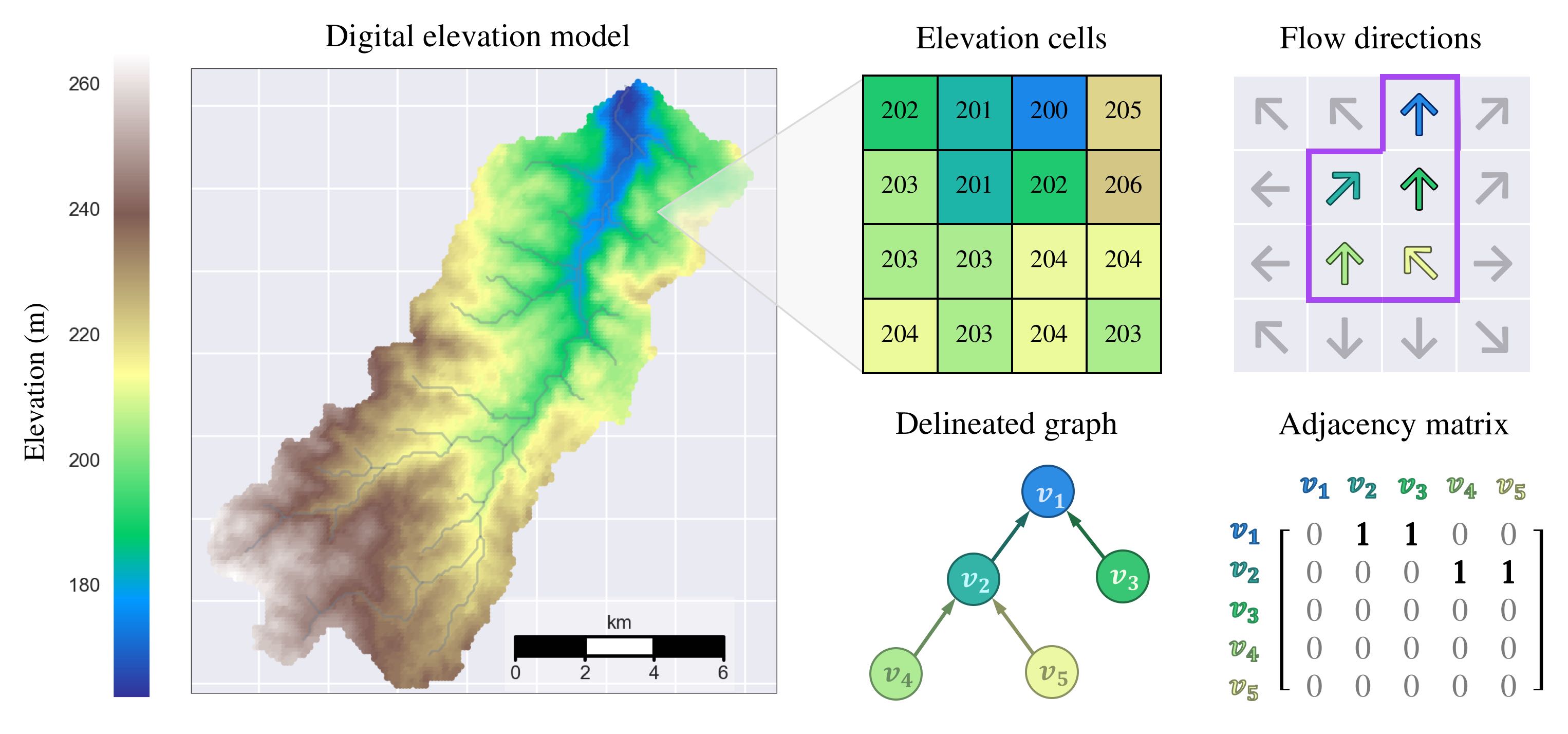
Figure 1: Left panel: Digital elevation model (DEM) of a watershed with river network highlighted. Right panel (from left to right, top to bottom): (i) DEM detail (colors not to scale); (ii) flow directions; (iii) delineated subcatchment graph; (iv) adjacency matrix representation of graph.

2.1 Definitions

Graph representation of a watershed: Watersheds can be represented as directed graphs, in which subcatchments (vertices or cells) are connected by elevation-dependent flow paths (edges). The directed graph can be formulated mathematically as an adjacency matrix, $A$, where for each element $a_{i,j}$, $a_{i,j}\neq 0$ if there exists a directed edge connecting vertex $v_{i}$ to $v_{j}$, and conversely, $a_{i,j}=0$ if there does not exist a directed edge connecting vertex $v_{i}$ to $v_{j}$. Nonzero edge weights can be specified to represent travel times, distances, or probabilities of transition between connected vertices. Flow paths between adjacent cells are established using a routing scheme, typically based on directions of steepest descent (see Figure 1).

In this study, we determine the connectivity of the drainage network using a D8 routing scheme [55]. In this scheme, elevation cells are treated as vertices in a 2-dimensional lattice (meaning that each vertex $v_{i}$ is surrounded by eight neighbors $\mathcal{N}_{i}$). A directed link is established from vertex $v_{i}$ to a neighboring vertex $v_{j}$ if the slope between $v_{i}$ and $v_{j}$ is steeper than the slope between $v_{i}$ and all of its other neighbors $\mathcal{N}_{i}\setminus v_{j}$ (where $v_{j}$ has a lower elevation than $v_{i}$). The D8 routing scheme produces a directed acyclic graph where the indegree of each vertex is between 0 and 8, and the outdegree of each vertex is 1, except for the watershed outlet, which is zero. It should be noted that other schemes exist for determining drainage network structure, such as the D-infinity routing algorithm, which better resolves drainage directions on hillslopes [56]. However, because the routing scheme is not essential to the construction of the algorithm, we focus on the simpler D8 routing scheme for this study. Similarly, to simplify the construction of the algorithm, we will assume that the vertices of the watershed are defined on a regular grid, such that the area of each unit subcatchment is equal. Figure 1 shows the result of delineating a river network from a digital elevation model (left), along with an illustration of the underlying graph structure and adjacency matrix representation (right).

Controller: In the context of this study, a controller represents any structure or practice that can regulate flows from an upstream channel segment to a downstream one. Examples include retention basins, dams, weirs, gates and other hydraulic control structures. These structures may be either passively or actively controlled. For the validation assessment presented later in this paper, we will examine the controller placement problem in the context of volume capture, meaning that controllers are passive, and that they are large enough to completely remove flows from their upstream contributing areas. However, the algorithm itself does not require the controller to meet these particular conditions.

Mathematically, we can think of a controller as a cut in the graph that removes one of the edges. This cut halts or inhibits flows across the affected edge. Because the watershed has a dendritic structure, any cut in the network will split the network into two sub-trees: (i) the delineated region upstream of the cut, and (ii) all the vertices that are not part of the delineated region. Placing controllers is thus equivalent to removing branches (subcatchments) from a tree (the parent watershed).

Delineation: Delineation returns the set of vertices upstream of a target vertex. In other words, this operation returns the contributing area of vertex $v_{i}$. Expressed in terms of the adjacency matrix:

$$\begin{split}V_{d}(A,v_{i})=\{v_{j}\in V|(A^{n})_{ij}\not=0\text{ for some }n\leq D\}\end{split}$$ (1)

Where $A^{n}$ is the adjacency matrix $A$ raised to the $n^{th}$ power, $i$ is the row index, $j$ is the column index, $V$ is the vertex set of $A$, and $D$ is the graph diameter. Note that $(A^{n})_{ij}$ is nonzero only if vertex $v_{j}$ is located within an n-hop neighborhood of vertex $v_{i}$.

Pruning: Pruning is the complement of delineation. This operation returns the vertex set consisting of all vertices that are not upstream of the current vertex.

$$V_{p}(A,v_{i})=V\setminus V_{d}(A,v_{i})$$ (2)

Subgraphs induced by the delineated and pruned vertex sets are defined as follows:

$$\begin{split}A_{d}(A,v_{i})=A(G[V_{d}])\\ A_{p}(A,v_{i})=A(G[V_{p}])\end{split}$$ (3)

Where $A(G[V])$ represents the adjacency matrix of the subgraph induced by the vertex set $V$.

Width function: The width function describes the distribution of travel times from each upstream vertex to some downstream vertex, $v_{i}$ [58]. In general terms, the width function can be expressed as:

$$H(t,v_{i})=\sum_{\gamma\in\Gamma_{i}}I(\gamma,t)$$ (4)

Along with an indicator function, $I(\gamma,t)$:

$$I(\gamma,t)=\begin{cases}1&T(\gamma)=t\\ 0&\text{otherwise}\end{cases}$$ (5)

Where $\Gamma_{i}$ is the set of all directed paths to the target vertex $v_{i}$, and $T(\gamma)$ is the travel time along path $\gamma$. If the travel times between vertices are constant, the width function of the graph at vertex $v_{i}$ can be described as a linear function of the adjacency matrix:

$$H(t,v_{i})=(A^{t}\mathbf{1})(i)$$ (6)

In real-world drainage networks, travel times between grid cells are not uniform. Crucially, the travel time for channelized cells will be roughly 1-2 orders of magnitude faster than the travel time in hillslope cells [58, 59]. Thus, to account for this discrepancy, we define $\phi$ to represent the ratio of hillslope to channel travel times:

$$\phi=\frac{t_{h}}{t_{c}}$$ (7)

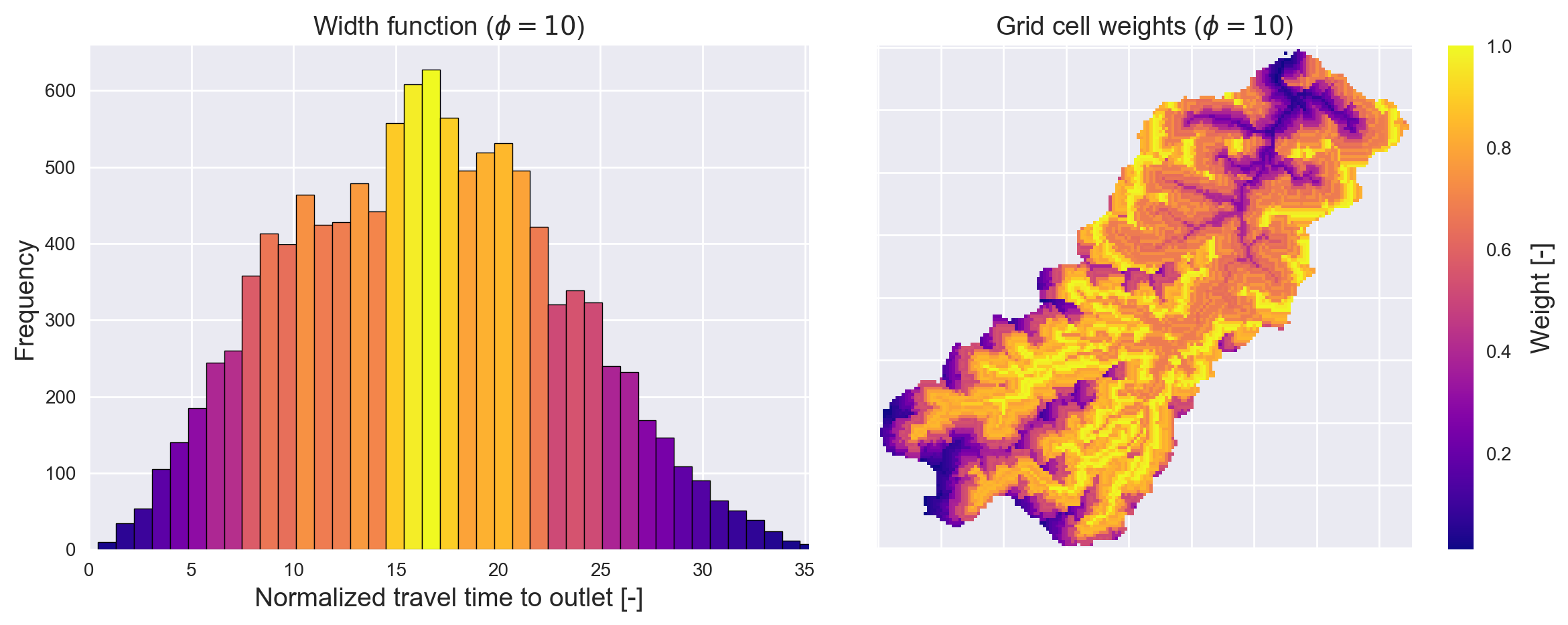
Figure 2: Left: width function (travel-time histogram) of the watershed, assuming that channelized travel time is ten times faster than on hillslopes ($\phi=10$). Right: weights associated with each vertex of the graph. Brighter regions correspond to areas that contribute to the peaks of the width function.

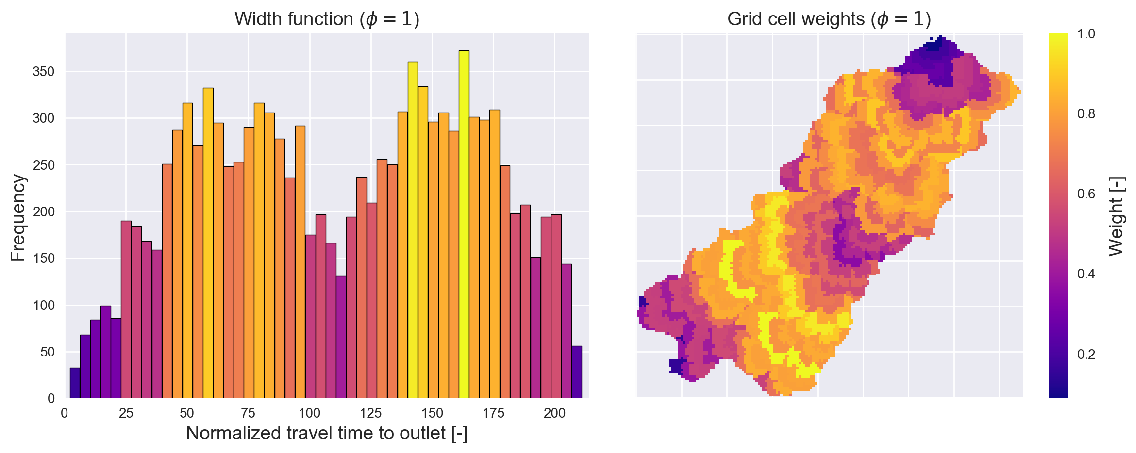
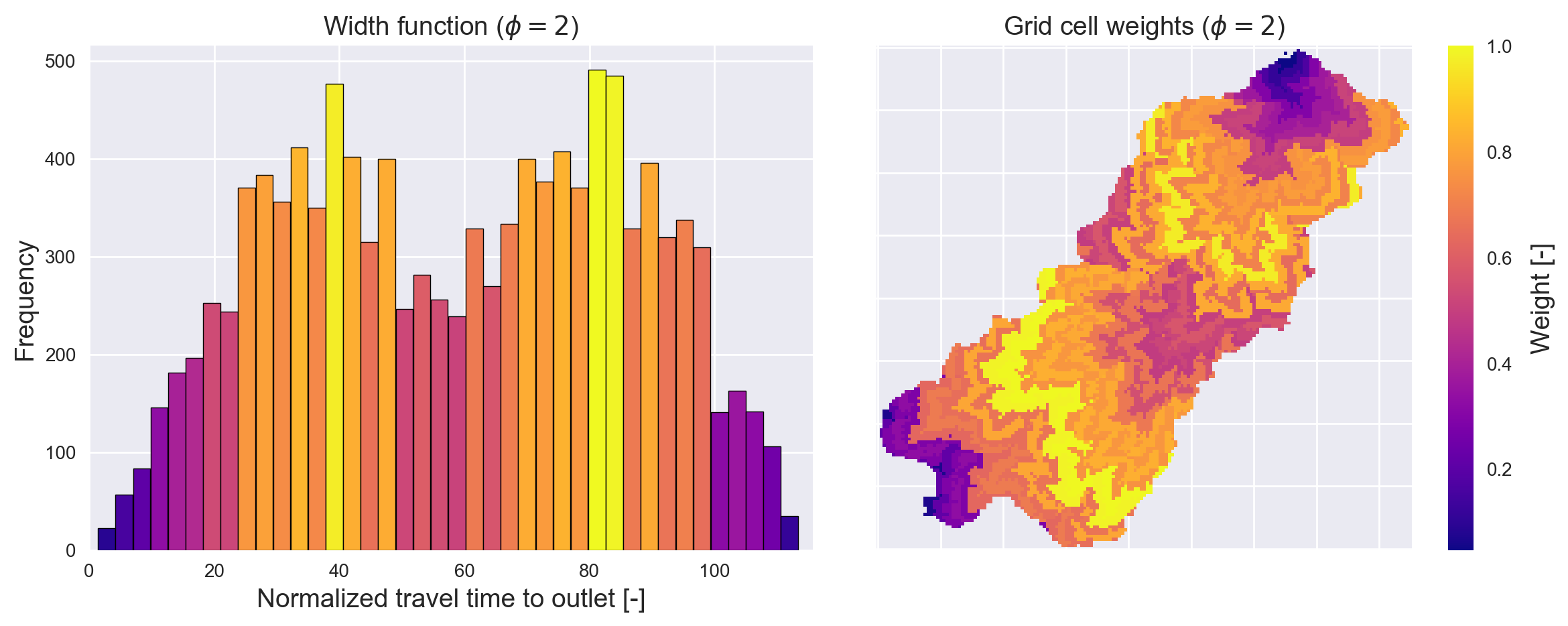
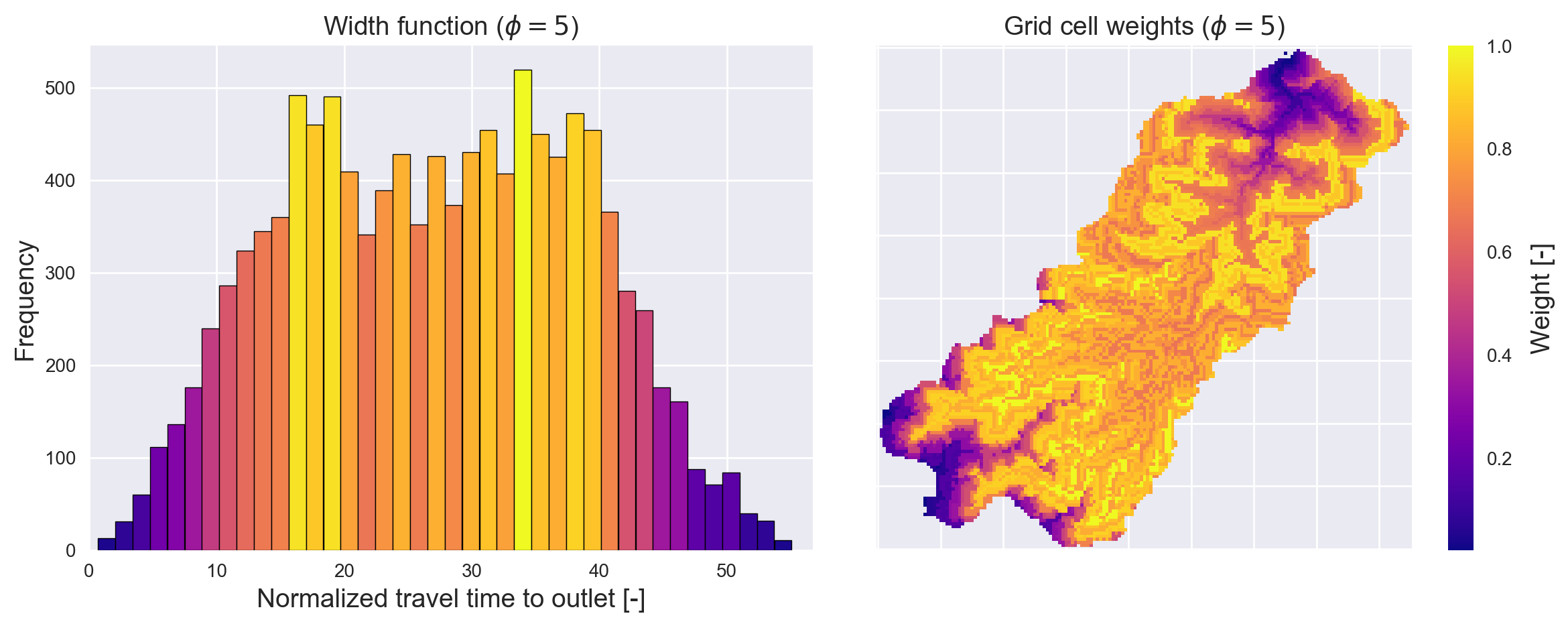
Figure S1: Width function (left) and vertex weights (right) as a function of $\phi$, with $\phi\in\{1,2,5\}$

Where $t_{h}$ is the travel time for hillslopes and $t_{c}$ is the travel time for channels. Figure 2 (left) shows the width function for an example watershed, under the assumption that channel velocity is ten times faster than hillslope velocity ($\phi=10$). The width functions for various values of $\phi$ are shown in Figures S1 and S2 in the Supplementary Information.

Note that when the effects of hydraulic dispersion are ignored, the width function is equivalent to the geomorphological impulse unit hydrograph (GIUH) of the basin [58]. The GIUH represents the response of the basin to an instantaneous impulse of rainfall distributed uniformly over the catchment; or equivalently, the probability that a particle injected randomly within the watershed at time $t=0$ exits the watershed through the outlet at time $t=t^{\prime}$.

Accumulation: The accumulation at vertex $v_{i}$ describes the number of vertices located upstream of $v_{i}$ (or alternatively, the upstream area [60]). It is equivalent to the cumulative sum of the width function with respect to time:

$$C(v_{i})=(\sum_{t=0}^{\infty}A^{t}\mathbf{1})(i)$$ (8)

Figure 3 (left) shows the accumulation at each vertex for an example catchment. Because upstream area is correlated with mean discharge [58], accumulation is frequently used to determine locations of channels within a drainage network [60].

Weighting function: To identify the vertices that contribute most to synchronous flows at the outlet, we propose a weighting function that weights each vertex by its rank in the travel time distribution. Let $\tau_{ij}$ represent the known travel time from a starting vertex $v_{j}$ to the outlet vertex $v_{i}$. Then the weight associated with vertex $v_{j}$ can be expressed in terms of a weighting function $W(v_{i},v_{j})$:

$$w_{j}=W(v_{i},v_{j})=\frac{H(\tau_{ij},v_{i})}{\underset{t}{\max}(H(v_{i}))}$$ (9)

Where $\tau_{ij}$ represents the travel time from vertex $v_{j}$ to vertex $v_{i}$, $H(\tau_{ij},v_{i})$ represents the width function for an outlet vertex $v_{i}$ evaluated at time $\tau_{ij}$, and the normalizing factor $\underset{t}{\max}(H(v_{i}))$ represents the maximum value of the width function over all time steps $t$. In this formulation, vertices are weighted by the rank of the associated travel time in the width function. Vertices that contribute to the maximum value of the width function (the mode of the travel time distribution) will receive the highest possible weight (unity), while vertices that contribute to the smallest values of the width function will receive small weights. In other words, vertices will be weighted in proportion to the number of vertices that share the same travel time to the outlet. Figure 2 shows the weights corresponding to each bin of the travel time distribution (left), along with the weights applied to each vertex (right). Weights for varying values of $\phi$ are shown in Figures S1 and S2 in the Supplementary Information.

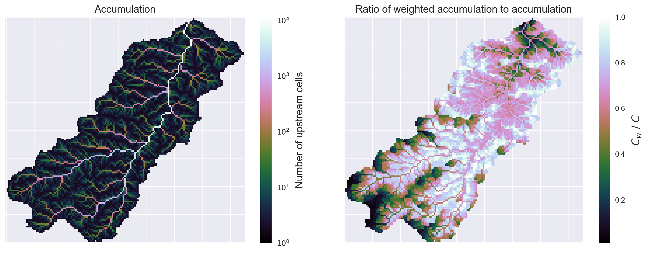
Figure 3: Left: accumulation (number of cells upstream of every cell). Right: ratio of weighted accumulation to accumulation ($C_{w}/C$).

Weighted accumulation: Much like the accumulation describes the number of vertices upstream of each vertex $v_{i}$, the weighted accumulation yields the sum of the weights upstream of $v_{i}$. If each vertex $v_{j}$ is given a weight $w_{j}$, the weighted accumulation at vertex $v_{i}$ can be defined:

$$C_{w}(v_{i},\mathbf{w})=(\sum_{t=0}^{\infty}A^{t}\mathbf{w})(i)$$ (10)

Where $\mathbf{w}$ is a vector of weights, with each weight $w_{j}$ associated with a vertex $v_{j}$ in the graph. When the previously-defined weighting function is used, the weighted accumulation score measures the extent to which a subcatchment delineated at vertex $v_{i}$ contributes to synchronous flows at the outlet. In other words, if the ratio of weighted accumulation to accumulation is large for a particular vertex, this means that the subcatchment upstream of that vertex contributes disproportionately to the peak of the hydrograph. Figure 3 (right) shows the ratio of weighted accumulation to accumulation for the example catchment. The weighted accumulation provides a natural metric for detecting the cuts in the drainage network that will maximally remove synchronous flows, and thus forms the basis of the controller placement algorithm.

2.2 Controller placement algorithm definition

The controller placement algorithm is described as follows. Let $A$ represent the adjacency matrix of a watershed delineated at some vertex $v_{i}$. Additionally, let $k$ equal the desired number of controllers, and $c$ equal the maximum upstream accumulation allowed for each controller. The graph is then partitioned according to the following scheme:

1. Compute the width function, $H(t,v_{i})$, for the graph described by adjacency matrix $A$ with an outlet at vertex $v_{i}$.

2. Compute the accumulation $C(v_{j})$ at each vertex $v_{j}$.

3. Use $H(t,v_{i})$ to compute the weighted accumulation $C_{w}(v_{j})$ at each vertex $v_{j}$.

4. Find the vertex $v_{opt}$, where the accumulation $C(v_{opt})$ is less than the maximum allowable accumulation and the weighted accumulation $C_{w}(v_{opt})$ is maximized:

   $$v_{opt}\leftarrow\underset{v_{s}\in V_{s}}{\text{argmax}}(C_{w}(v_{s}))$$ (11)

   Where $V_{s}$ is the set of vertices such that vertex $v_{i}$ is reachable from any vertex in $V_{s}$ and the accumulation $C$ at any vertex in $V_{s}$ is less than $c$.

5. Prune the graph at vertex $v_{opt}$: $A\leftarrow A_{p}(A,v_{opt})$

6. If the cumulative number of partitions is equal to $k$, end the algorithm. Otherwise, start at (1) with the catchment described by the new $A$ matrix.

The algorithm is described formally in Algorithm 1. An open-source implementation of the algorithm in the Python programming language is also provided [61], along with the data needed to reproduce our results. Efficient implementations of the delineation, accumulation, and width function operations are provided via the pysheds toolkit, which is maintained by the authors [62].

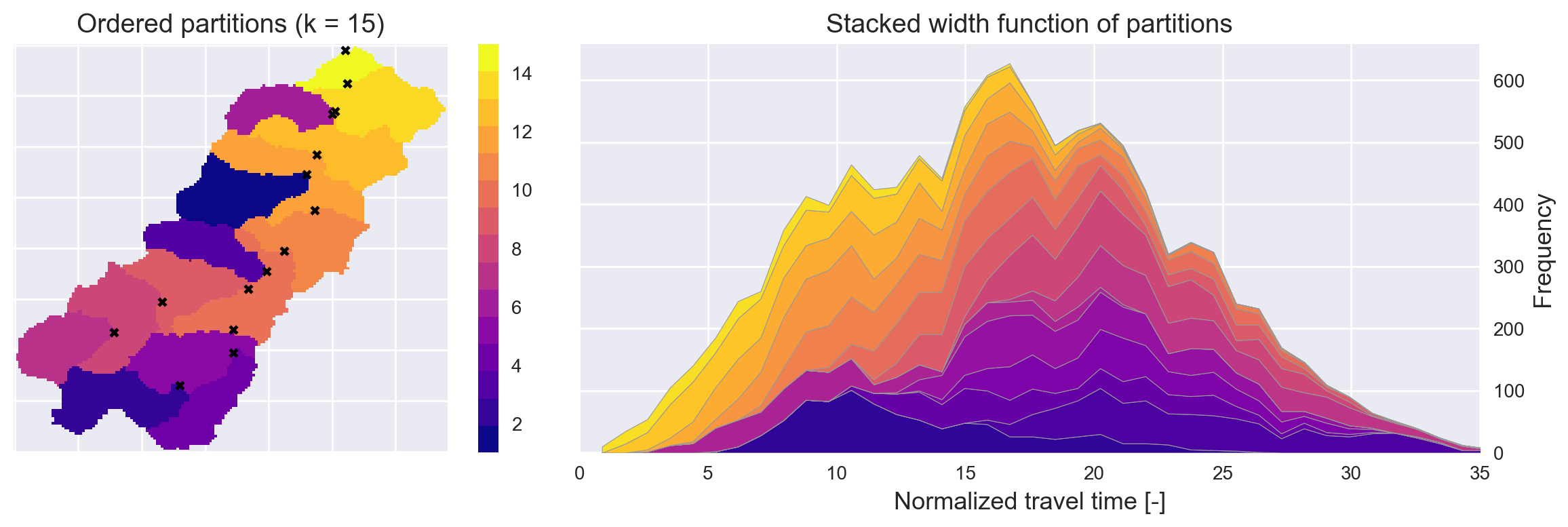
Figure 4: Left: partitioning of the example watershed using the controller placement algorithm. Right: stacked width functions for each partition. The brightness expresses the priority of each partition, with the darker partitions being prioritized over the brighter ones.

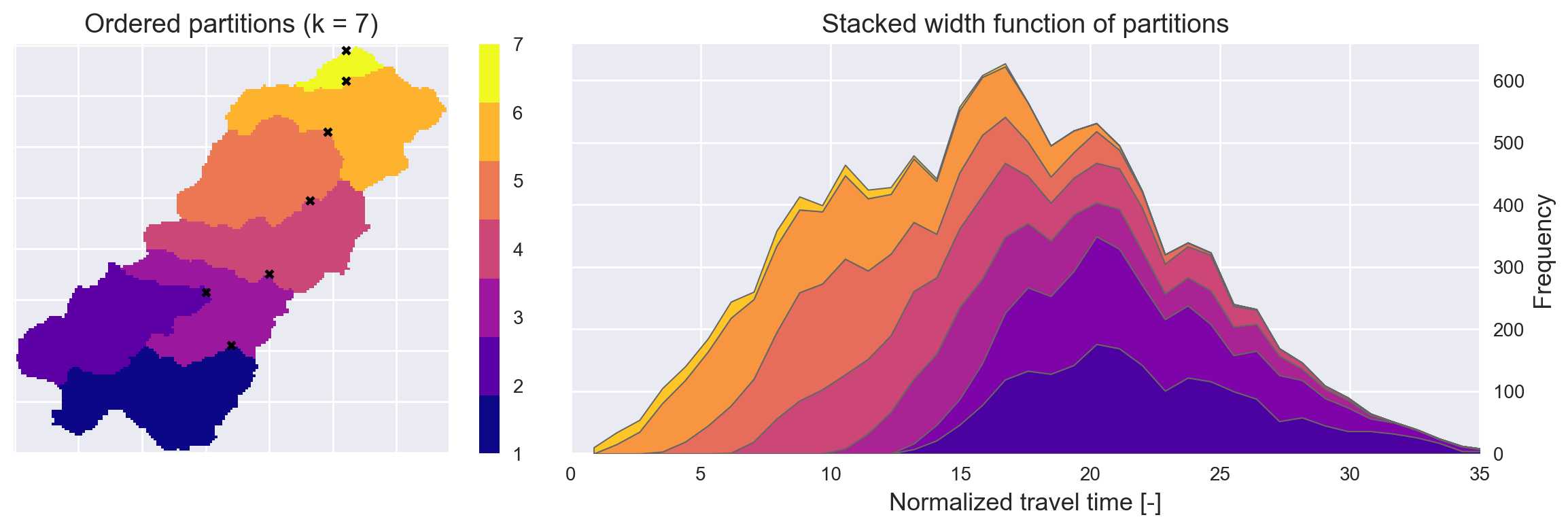
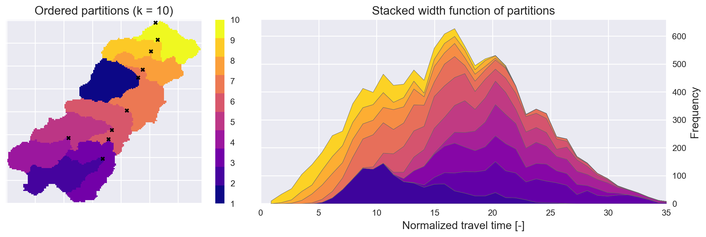
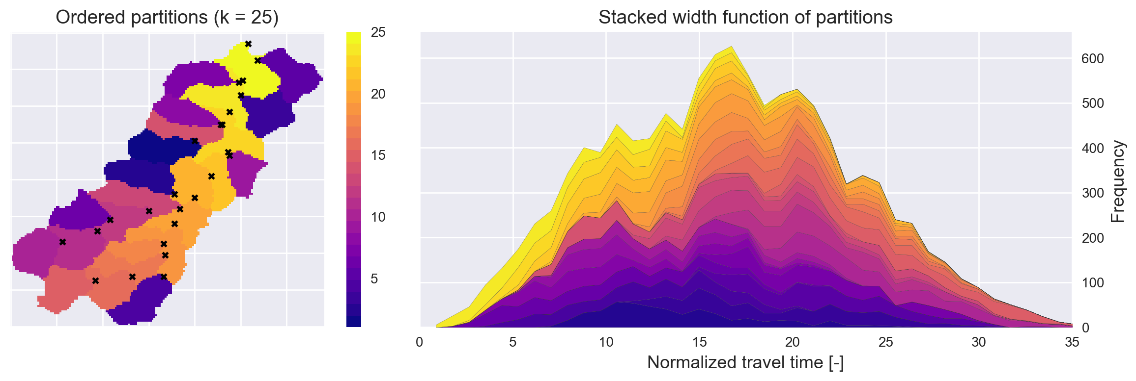
Figure S3: Optimized controller placements (left) and stacked width functions for varying number of controllers (right), $k\in\{7,10,25\}$, $\phi=10$.

Figure 4 shows the controller configuration generated by applying the controller placement algorithm to the example watershed, with $k=15$ controllers, each with a maximum accumulation of $c=900$ (i.e. each controller captures roughly 8% of the catchment’s land area). In the left panel, partitions are shown in order of decreasing priority from dark to light (i.e. darker regions are partitioned first by the algorithm). The right panel shows the stacked width functions for each partition. The sum of the width functions from each partition reconstitute the original width function for the catchment. From the stacked width functions, it can be seen that the algorithm tends to prioritize the pruning of subgraphs that align with the peaks of the travel time distribution. Note for instance, how the least-prioritized paritions gravitate towards the low end of the travel-time distribution, while the most-prioritized partitions are centered around the mode. Controller placement schemes corresponding to different numbers of controllers are shown in Figure S3 in the Supplementary Information.

A directed graph described by adjacency matrix $A$;

A target vertex $v_{i}$ with index $i$;

A desired number of partitions $k$;

The maximum accumulation at each controller, $c$;

Result: Generate partitions for a catchment

Let $\mathbf{q}$ be a vector representing all vertices in the graph;

Let $k_{c}$ equal the current number of partitions;

Let $\mathbf{\tau}$ represent a vector of travel times from each vertex to vertex $v_{i}$;

Let $A$ represent the adjacency matrix of the system;

Let $A_{c}$ represent the adjacency matrix for the current iteration;

$A_{c}\leftarrow A$;

$k_{c}\leftarrow 0$;

while $k_{c}<k$ do

      

      $H(t,v_{i})\leftarrow(A_{c}^{t}\mathbf{1})(i)$;

       $C\leftarrow(\sum_{t=0}^{\infty}A_{c}^{t}\mathbf{1})$;

       $\mathbf{w}\leftarrow W(v_{i},\mathbf{q})$;

       $C_{w}\leftarrow(\sum_{t=0}^{\infty}A_{c}^{t}\mathbf{w})$;

      

      if $C(v_{i})>0$ then

             $V_{c}\leftarrow\{v_{m}\in V|C(v_{m})\leq c\}$;

             $V_{s}\leftarrow V_{d}(A_{c},v_{i})\cap V_{c}$;

             $v_{opt}\leftarrow\underset{v_{s}\in V_{s}}{\text{argmax}}(C_{w}(v_{s}))$;

             $A_{c}\leftarrow A_{p}(A_{c},v_{opt})$;

             $k_{c}\leftarrow k_{c}+1$;

            

      else

            

       end if

      

end while

Algorithm 1 Controller placement algorithm

3 Algorithm validation

To evaluate the controller placement algorithm, we simulate the controlled network using a hydrodynamic model, and compare the performance to a series of randomized controller placement configurations. Performance is characterized by the “flatness” of the flow profile at the outlet of the watershed, as measured by both the peak discharge and the variance of the hydrograph (i.e. the extent to which the flow deviates from the mean flow over the course of the hydrologic response). To establish a basis for comparison, we simulate a volume capture scenario [21], wherein roughly half of the total contributing area is controlled, and each controller completely captures the discharge from its respective upstream area.

The validation experiment is designed to test the central premises of the controller placement algorithm: that synchronous cells can be identified from the structure of the drainage network, and that maximally capturing these synchronous cells will lead to a flatter overall hydrologic response. If these premises are accurate, we expect to see two results. First, the controller placement algorithm will produce flatter flows than the randomized control trials. Second, the performance of the algorithm will be maximized when using a large number of small partitions. Using many small partitions allows the algorithm to selectively target the highly-weighted cells that contribute disproportionately to the peak of the hydrograph. Conversely, large partitions capture many extraneous low-weight cells that don’t contribute to the peak of the hydrograph. In other words, if increasing the number of partitions improves the performance of the algorithm, it not only confirms that the algorithm works for our particular experiment, but also justifies the central premises on which the algorithm is based.

3.1 Experimental design

We evaluate controller configurations based on their ability to flatten the outlet hydrograph of a test watershed when approximately 50% of the contributing area is controlled. This test case is chosen because it presents a practical scenario with real-world constraints, and because it allows for direct comparison of many different controller placement strategies. For our test case, we use the Sycamore Creek watershed, a heavily urbanized creekshed located in the Dallas–Fort Worth Metroplex with a contributing area of roughly 83 km² (see Figure 1). This site is the subject of a long-term monitoring study led by the authors [17], and is chosen for this analysis because (i) it is known to experience issues with flash flooding, and (ii) it is an appropriate size for our analysis—being large enough to capture fine-scale network topology, but not so large that computation time becomes burdensome.

A model of the stream network is generated from a conditioned digital elevation model (DEM) by determining flow directions from the elevation gradient and then assigning channels to cells that fall above an accumulation threshold. Conditioned DEMs and flow direction grids at a resolution of 3 arcseconds (approximately 70 by 90 m) are obtained from the USGS HydroSHEDS database [63]. Grid cells with an accumulation greater than 100 are defined to be channelized cells, while those with less than 100 accumulation are defined as hillslope cells. This threshold is based on visual comparison with the stream network defined in the National Hydrography Dataset (NHD) [64]. Hillslope cells draining into a common channel are aggregated into subcatchments, with a flow length corresponding to the longest path within each hillslope, and a slope corresponding to the average slope over all flow paths in the subcatchment. To avoid additional complications associated with modeling infiltration, subcatchments and channels are assumed to be completely impervious. Channel geometries are assigned to each link within the channelized portion of the drainage network. We assume that each stream segment can be represented by a “wide rectangular channel”, which is generally accurate for natural river reaches in which the stream width is large compared to the stream depth [65]. To simulate channel width and depth, we assume a power law relation between accumulation and channel size based on an empirical formulation from Moody and Troutman (2002) [66]:

$$\begin{split}\omega=7.2\cdot Q^{0.50\pm 0.02}\\ h=0.27\cdot Q^{0.30\pm 0.01}\end{split}$$ (12)

Where $\omega$ is stream width, $h$ is stream depth, and $Q$ is the mean river discharge. Knowing the width and depth of the most downstream reach, and assuming that the accumulation at a vertex is proportional to the mean flow, we generate channel geometries using the mean parameter values from the above relations.

Using the controller placement algorithm, control structures are placed such that approximately 50$\pm$3% of the catchment area is captured by storage basins. To investigate the effect of the number of controllers on performance, optimized controller strategies are generated using between $k=1$ and $k=35$ controllers. The ratio of hillslope-to-channel travel times is assumed to be $\phi=10$. We compare the performance of our controller placement algorithm to randomized controller placement schemes, in which approximately 50$\pm$3% of the catchment area is controlled but the placement of controllers is random. For this comparison assessment, we generate 50 randomized controller placement trials, each using between $k=1$ and $k=24$ controllers.

We simulate the hydrologic response using a hydrodynamic model, and evaluate controller placement performance based on the flatness of the resulting hydrograph. To capture the hydrologic response under various rainfall conditions, we simulate small, medium and large rainfall events, corresponding to 0.5, 1.5 and 4.0 mm of rainfall delivered instantaneously over the first five minutes of the simulation. A hydrodynamic model is used to simulate the hydrologic response at the outlet by routing runoff through the channel network using the dynamic wave equations [67]. The simulation performance is measured by both the peak discharge and the total variance of the hydrograph. The variance of the hydrograph (which we refer to as “flashiness”) is defined as:

$$\sigma^{2}=\frac{1}{N}\sum_{i=1}^{N}(Q_{i}-\bar{Q})^{2}$$ (13)

Where $Q$ is the discharge, $\bar{Q}$ is the mean discharge in the storm window, and $N$ is the number of data points in the storm window. This variance metric captures the flow’s deviation from the mean over the course of the hydrologic response, and thus provides a natural metric for the flatness of the hydrograph. This metric is important for water quality considerations like first flush contamination or streambed erosion—in which the volume of transported material (e.g. contaminants or sediments) depends not only on the maximum discharge, but also on the duration of flow over a critical threshold [68].

Note that the validation experiment is not intended to faithfully reproduce the precise hydrologic response of our chosen study area, but rather, to test the basic premises of the controller placement algorithm. As such, site-specific details—such as land cover, soil types and existing infrastructure—have been deliberately simplified. For situations in which these characteristics exert an important influence on the hydrologic response, one may account for these factors by adjusting the inter-vertex travel times used in the controller placement algorithm.

4 Results

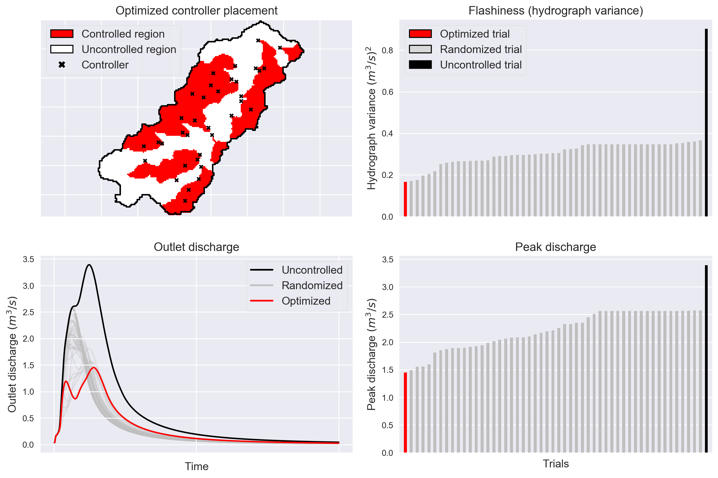
Figure 5: Results of the hydraulic simulation experiment for the medium storm event (1.5 mm). Top left: optimal controller placement ($k=35$), with captured regions in red. Bottom left: hydrographs resulting from each simulation. The uncontrolled simulation is shown in black, while the optimized controller placement simulations are shown in red, and the randomized controller simulations are shown in gray. Right: the overall flashiness (variance of the hydrograph) and peak discharge for each simulation, using the same coloring scheme.

The controller placement algorithm produces consistently flatter flows than randomized control trials. Figure 5 shows the results of the hydraulic simulation assessment in terms of the resulting hydrographs (bottom left), and the overall flashiness and peak discharge of each simulation (right) for the medium-sized (1.5 mm) storm event. The best performance is achieved by using the controller placement algorithm with $k=35$ controllers (see Figure 5, top left). Comparing the overall variances and peak discharges, it can be seen that the optimized controller placement produces flatter outlet discharges than any of the randomized controller placement strategies. Specifically, the optimized controller placement achieves a peak discharge that is roughly 47% of that of the uncontrolled case, while the randomized simulations by comparison achieve an average peak discharge that is more than 72% of that of the uncontrolled case. Similarly, the hydrograph variance of the optimized controller placement is roughly 21% of that of the uncontrolled case, compared to 35% for the randomized simulations on average. When tested against storm events of different sizes (0.5 to 4 mm of rain), the controller placement algorithm also generally outperforms randomized control trials (see Section S4 in the Supplementary Information). However, the within-group performance varies slightly with rain event size, which could result from the nonlinearities inherent in wave propagation speed. Thus, while the optimized controller placement still produces flatter flows than randomized controls, this result suggests that the performance of the controller placement algorithm could be further improved by tuning the assumed inter-vertex travel times to correspond to the expected speed of wave propagation.

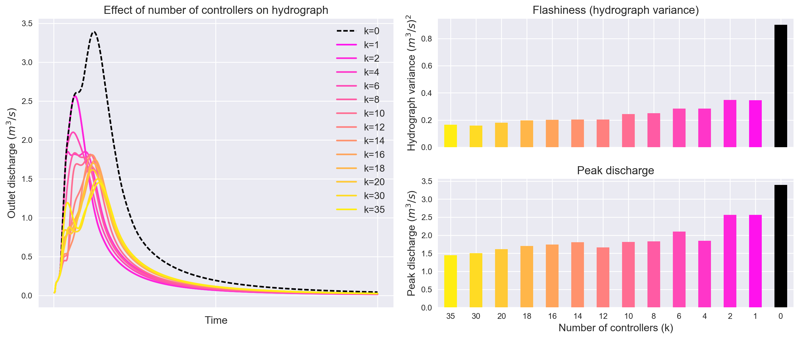
Figure 6: Left: hydrographs associated with varying numbers of controllers (k), using the controller placement algorithm with 50% watershed area removal. Right: hydrograph variance (top) and peak discharge (bottom) vs. number of controllers. In general, more controllers produces a flatter response.

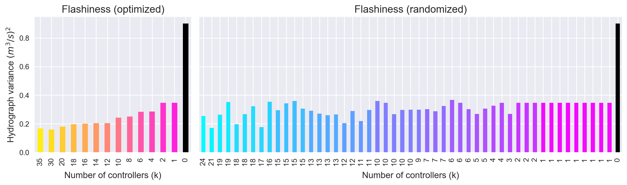
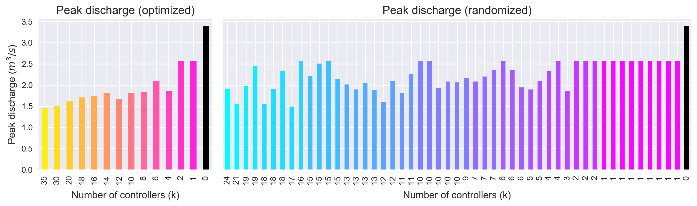
Figure S8: Performance metrics for both optimized (left) and randomized (right) controller placements by number of controllers used. The top panel measures performance in terms of flashiness (hydrograph variance), while the bottom panel measures performance by peak discharge. The optimized controller placements show consistently better performance metrics as the number of controllers is increased, while the randomized simulations do not.

Under the controller placement algorithm, the best performance is achieved by using a large number of small-scale controllers; however, more controllers does not lead to better performance for the randomized controller placement scheme. Given that increasing the number of controllers allows the algorithm to better target highly synchronous cells, this result is consistent with the central premise that capturing synchronous cells will lead to a flatter hydrologic response. Figure 6 shows the optimized hydrologic response for varying numbers of controllers (left), along with the overall variance (top right) and peak discharge (bottom right). In all cases, roughly 50% of the watershed is controlled; however, configurations using many small controllers consistently perform better than configurations using a few large controllers. This trend does not hold for the randomized controller placement strategy (see Figure S8 in the Supplementary Information). Indeed, the worst-performing randomized controller placement uses $k=6$ controllers (out of a minimum of 1) while the best-performing randomized controller placement uses $k=18$ controllers (out of a maximum of 24). The finding that the controller placement algorithm converges to a (locally) optimal solution follows from the fact that as the number of partitions increases, controllers are better able to capture highly-weighted regions without also capturing extraneous low-weight cells. This in turn implies that the weighting scheme used by the algorithm accurately identifies the regions of the watershed that contribute disproportionately to synchronized flows. Thus, in spite of various sources of model and parameter uncertainty, the experimental results confirm the central principles under which the controller placement algorithm operates: namely, that synchronous regions can be deduced from the graph structure alone, and that controlling these regions results in a flatter hydrograph compared to randomized controls.

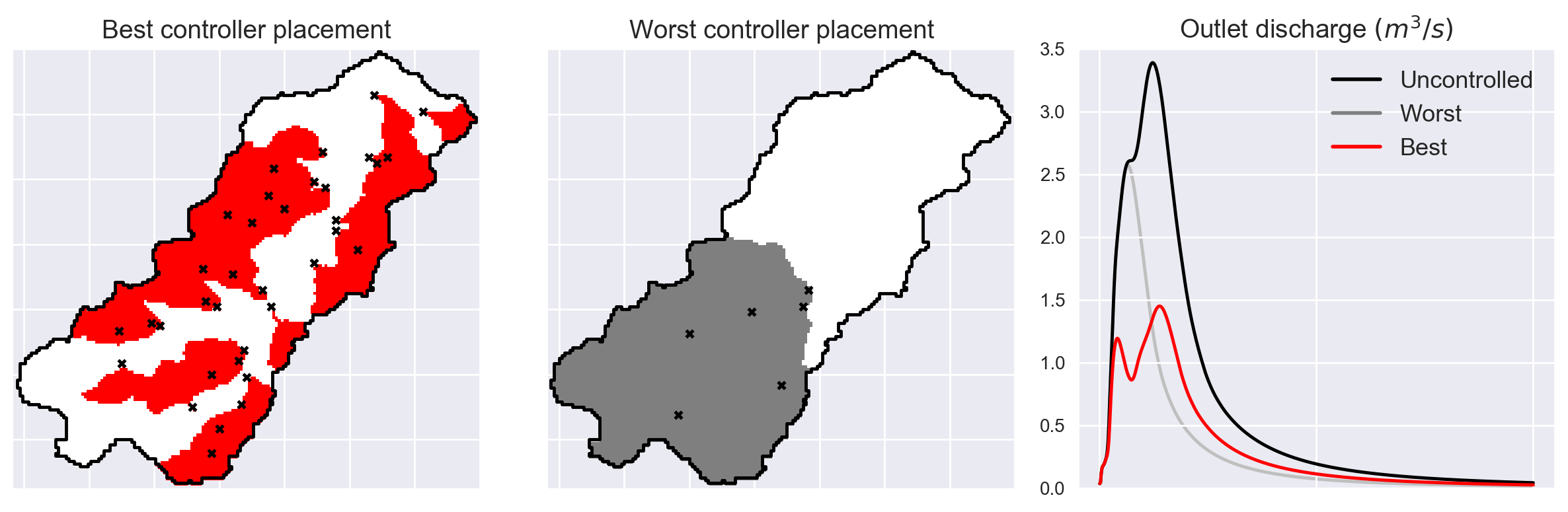
Figure 7: Left: Best controller placement in terms of peak discharge ($k=35$ controllers, optimized). Center: worst controller placement in terms of peak discharge ($k=6$ controllers, randomized). Controller locations are indicated by black crosses, and controlled partitions are indicated by colored regions. Right: hydrographs associated with the best and worst controller placement strategies.

In addition to demonstrating the efficacy of the controller placement algorithm, the validation experiments reveal some general principles for organizing hydraulic control structures within drainage networks to achieve downstream streamflow objectives. Overall, the controller placement strategies that perform best—whether achieved through optimization or randomization—tend to partition the watershed axially rather than laterally. These lengthwise partitions result in a long, thin drainage network that prevents tributary flows from “piling up”. Figure 7 shows the partitions corresponding to the best-performing and worst-performing controller placement strategies with respect to peak discharge (left and center, respectively), along with the associated hydrographs (right). While the best-performing controller placement strategy evenly distributes the partitions along the length of the watershed, the worst-performing controller placement strategy controls only the most upstream half of the watershed. As a result, the worst-performing strategy removes the largest part of the peak, but completely misses the portion of the peak originating from the downstream half of the watershed. In order to achieve a flat downstream hydrograph, controller placement strategies should seek to evenly distribute controllers along the length of the watershed.

5 Discussion

The controller placement algorithm presented in this study provides a tool for designing stormwater control systems to better mitigate floods, regulate contaminants, and protect aquatic ecosystems. By reducing peak discharge, optimized placement of stormwater control structures may help to lessen the impact of flash floods. Existing flood control measures often focus on controlling large riverine floods—typically through existing centralized assets, like dams and levees. However, flash floods may occur in small tributaries, canals, and even normally dry areas. For this reason, flash floods are not typically addressed by large-scale flood control measures, despite the fact that they cause more fatalities than riverine floods in the developed world [2]. By facilitating distributed control of urban flash floods, our controller placement strategy could help reduce flash flood related mortality. Moreover, by flattening the hydrologic response, our controller placement algorithm promises to deliver a number of environmental and water quality benefits, such as decreased first flush contamination [68], decreased sediment transport [69], improved potential for treatment in downstream green infrastructure [1, 17], and regulation of flows in sensitive aquatic ecosystems [70].

5.1 Key features of the algorithm

The controller placement algorithm satisfies a number of important operational considerations:

• Theoretically motivated. The controller placement algorithm has its foundation in the theory of the geomorphological impulse unit hydrograph—a relatively mature theory supported by a established body of research [58, 26, 27, 28, 29, 30, 31]. Moreover, the algorithm works in an intuitive way—by recursively removing the subcatchments of a watershed that contribute most to synchronized flows. This theoretical basis distinguishes our algorithm from other strategies that involve exhaustive optimization or direct application of existing graph theoretical constructs (such as graph centrality metrics).

• Generalizable and extensible. Because it relies solely on network topology, the controller placement algorithm will provide consistent results for any drainage network—including both natural stream networks and constructed sewer systems. Moreover, because each step in our algorithm has a clear meaning in terms of the underlying hydrology, the algorithm can be modified to satisfy more complex control problems (such as systems in which specific regulatory requirements must be met).

• Flexible to user objectives and constraints. The controller placement algorithm permits specification of important practical constraints, such as the amount of drainage area that each control site can capture, and the number of control sites available. Moreover, the weighting function can be adjusted to optimize for a variety of objectives (such as the overall “flatness” of the hydrograph, or removal of flows from a contaminated upstream region).

• Parsimonious with respect to data requirements. The controller placement algorithm requires only a digital elevation model of the watershed of interest. Additional data—such as land cover and existing hydraulic infrastructure—can be used to fine-tune estimates of travel times within the drainage network, but are not required by the algorithm itself.

• Fast implementation For the watershed examined in this study (consisting of about 12,000 vertices), the controller placement algorithm computes optimal locations for $k=15$ controllers in roughly 3.0 seconds (on a 2.9 GHz Intel Core i5 processor). While the computational complexity of the algorithm is difficult to characterize, it is faster than other comparable graph-cutting algorithms, such as recursive spectral bisection or spectral clustering, both of which are $O(n^{3})$ in computational complexity.

Taken together, our algorithm offers a solution to the controller placement problem that is suitable for research as well as for practical applications. On one hand, the algorithm is based in hydrologic and geomorphological theory, and provides important insights into the connections between geomorphology and the design of the built environment. On the other hand, the algorithm is fast, robust, and easy-to-use, making it a useful tool for practicing engineers and water resource managers.

5.2 Caveats and directions for future research

While our controller placement algorithm is robust and broadly-applicable, there are a number of important considerations to keep in mind when applying this algorithm to real-world problems.

• The controller placement algorithm implicitly assumes that rainfall is uniform over the catchment of interest. While this assumption is justified for small catchments in which the average spatial distribution of rainfall will be roughly uniform, this assumption may not hold for large (e.g. continent-scale) watersheds. Modifications to the algorithm would be necessary to account for a non-uniform spatial distribution of rainfall.

• The controller placement algorithm is sensitive to the chosen ratio of hillslope to channel speeds, $\phi$. Care should be taken to select an appropriate value of $\phi$ based on site-specific land cover and morphological characteristics. More generally, for situations in which differential land cover, soil types, and existing hydraulic infrastructure play a dominating role, the performance of the algorithm may be enhanced by adjusting inter-vertex travel times to correspond to estimated overland flow and channel velocities.

• Our assessment of the algorithm’s performance rests on the assumption that installed control structures (e.g. retention basins) are large enough to capture upstream discharges. The algorithm itself does not explicitly account for endogenous upstream flooding that could be introduced by installing new control sites.

• In this study, experiments were conducted only for impulsive rainfall inputs (i.e. with a short duration of rainfall). Future work should assess the performance of the distance-weighted controller placement strategy under arbitrary rainfall durations.

More broadly, future research should investigate the problem of sensor placement in stream networks using the theoretical framework developed in this paper. While this study focuses on the problem of optimal placement of hydraulic control structures, our algorithm also suggests a solution to the problem of sensor placement. Stated probabilistically, the geomorphological impulse unit hydrograph (GIUH) represents the probability that a “particle” injected randomly within the watershed at time $t=0$ exits the outlet at time $t=t^{\prime}$. Thus, the peaks of the GIUH correspond to the portions of the hydrologic response where there is the greatest amount of ambiguity about where a given “particle” originated. It follows that the same locations that maximally de-synchronize flows may also be the best locations for disambiguating the locations from which synchronous flows originated. Future experiments should investigate the ability to estimate upstream states (e.g. flows) within the network given an outlet discharge along with internal state observers (e.g. flow sensors) placed using the algorithm developed in this study.

6 Conclusions

We develop an algorithm for placement of hydraulic control structures that maximally flattens the hydrologic response of drainage networks. This algorithm uses the geomorphological impulse unit hydrograph to locate subcatchments that dominate the peaks of the hydrograph, then partitions the drainage network to minimize the contribution of these subcatchments. We find that the controller placement algorithm produces flatter hydrographs than randomized controller placement trials—both in terms of peak discharge and overall variance. By reducing the flashiness of the hydrologic response, our controller placement algorithm may one day help to mitigate flash floods and restore urban water quality through reduction of contaminant loads and prevention of streambed erosion. We find that the performance of the algorithm is enhanced when using a large number of small, distributed controllers. In addition to confirming the central hypothesis that synchronous cells can be identified based on network structure of drainage basins, this result lends justification to the development of decentralized smart stormwater systems, in which active control of small-scale retention basins, canals and culverts enables more effective management of urban stormwater. Overall, our algorithm is efficient, requires only digital elevation model data, and is robust to parameter and model uncertainty, making it suitable both as a research tool, and as a design tool for practicing water resources engineers.

Declarations of interest

Declarations of interest: none.

Data availability

Upon publication, code and data links will be made available at:

https://github.com/kLabUM/hydraulic-controller-placement

References

Supplementary information

S1 Implementations of algorithms used in the study

S1.1 Width function

For the software implementation used in this study, the width function is computed by determining the travel times from each vertex to the outlet, and then generating a binned histogram of these travel times. The travel times from each vertex to the outlet are computed by performing a depth-first search on the graph representation of the watershed starting with the outlet, and then recording the distances from each vertex to the outlet. The travel times are then binned to produce the width function. The travel time computation is implemented as grid.flow_distance in the pysheds software package, available at github.com/mdbartos/pysheds.

Note that if matrix multiplication is used to compute the width function, the inter-vertex travel times cannot be used as the weights of the adjacency matrix. Rather, differential travel times may be accounted for by modifying the topology of the graph. For instance, consider a graph consisting of fast nodes and slow nodes, where fast nodes transfer flow 10 times as quickly as slow nodes. In this scheme, slow nodes can be modeled using 10 “dummy” vertices placed in series. It should be noted however, that this implementation is inefficient both in terms of speed of computation and memory usage.

S1.2 Flow accumulation

The vectorized flow accumulation algorithm (developed previously by the authors, but unpublished) is reproduced here for the reader’s convenience:

1. Create an m x n array, edges to represent the edges of the directed graph. For each entry in the array, the index corresponds to the index of the start node, and the value corresponds to the index of the end node.

2. Create an m x n array, in_degree, to hold the in-degree of each grid cell (i.e. the number of cells currently pointing to that cell). This can be accomplished by counting the number of occurrences of each unique value in edges.

3. Create an m x n array of ones flow_accumulation to hold the computed number of upstream cells for each cell.

4. Define a 1 x nm array startnodes with entries equal to the indices of edges.

5. Define a 1 x nm array endnodes with entries equal to the values of edges.

6. Create a 1 x nm boolean index no_predecessors which is 0 where in_degree is greater than 0, and 1 where in_degree is equal to zero.

7. Select the subset of start nodes and end nodes that have no predecessors: startnodes = startnodes[no_predecessors] and endnodes = endnodes[no_predecessors]. This selects the “outermost layer” of nodes.

8. While endnodes is not empty:

   • Add the flow accumulation at the start nodes to the flow accumulation of the end nodes: flow_accumulation[endnodes] += flow_accumulation[startnodes]

   • Decrement the in-degree of the endnodes by the number of start nodes that are linked to it in the current step. With endnodes containing repeated entries this operation can be represented as: in_degree[endnodes] -= 1.

   • Set the new value of startnodes as the unique elements in endnodes with a current in-degree of zero: startnodes = unique(endnodes)[(in_degree == 0)]

   • Set endnodes as the end nodes corresponding to the new start nodes: endnodes = edges[startnodes].

This algorithm is implemented as grid.accumulation in the pysheds software package, available at github.com/mdbartos/pysheds.

S2 Vertex weights as a function of $\phi$

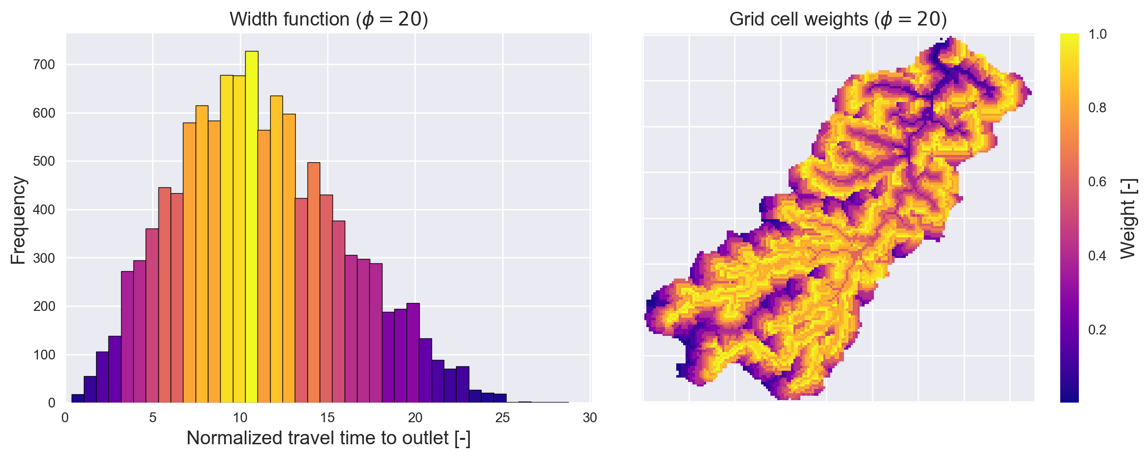
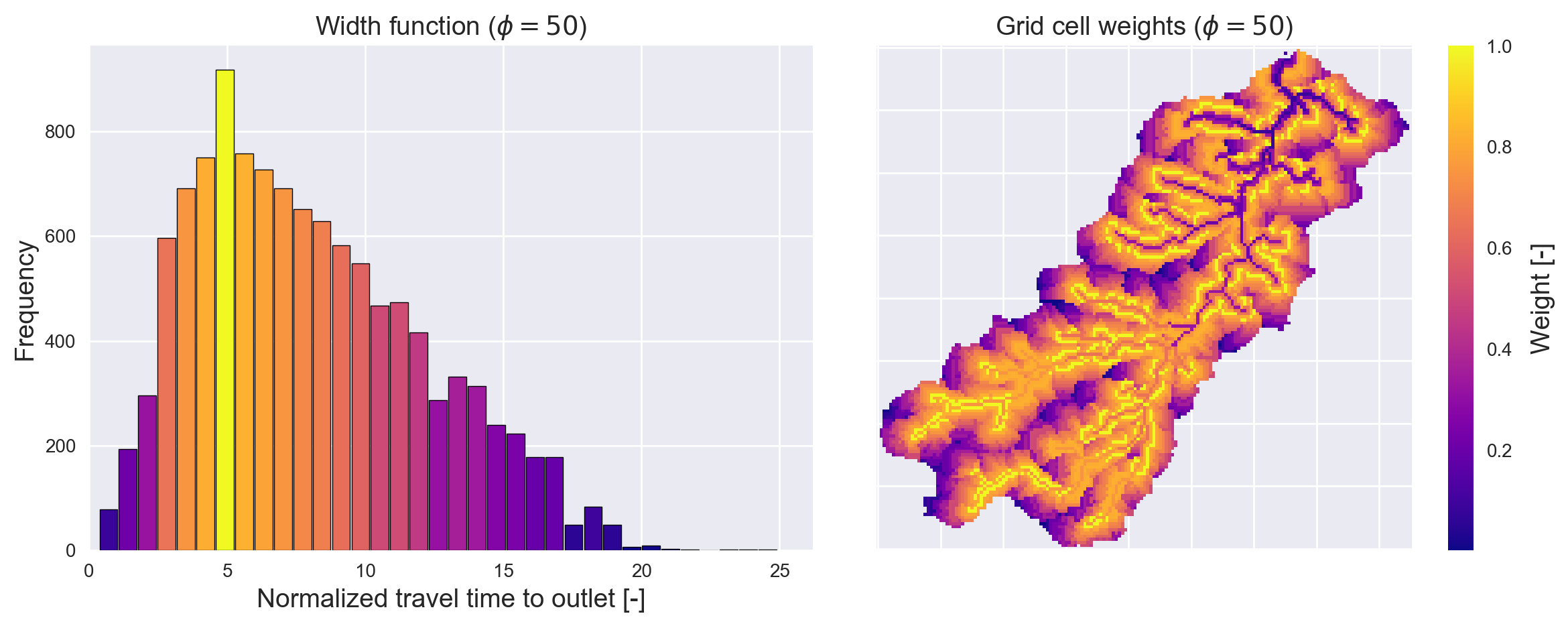
Figure S2: Width function (left) and vertex weights (right) as a function of $\phi$, with $\phi\in\{10,20,50\}$

S3 Optimal controller placements for various numbers of controllers ($k$)

S4 Performance under rainfall events of different sizes

When tested against storm events of different sizes, the controller placement algorithm generally outperforms randomized control trials. However, the relative performance between simulations varies with rainfall intensity, which suggests that a uniquely optimal controller placement may not exist for rainfall events of all sizes. As shown in Figures S4 and S5, the optimized controller placement still produces flatter flows overall compared to randomized trials for the small and large storm events. However, for the large storm event, one of the randomized simulations produces a slightly smaller peak discharge than the best-performing optimized controller placement. Moreover, the within-group performance of controller placement strategies varies with storm event size, as seen in Figures S6 and S7. For instance, the controller placement that produces the smallest peak discharge under the large storm event produces the 4th smallest peak discharge under the medium storm event, and the 7th smallest peak discharge under the small storm event (Figure S7). These results suggest that the optimal controller placement for large storms may not be the same as the optimal controller placement for small storms. This situation may result from the fact that larger flood waves travel faster, meaning that inter-vertex travel times will change depending on the scale of the hydrologic response. Consequently, assumed inter-vertex travel times (controlled in this experiment by the parameter $\phi$) may need to be tuned depending on storm event size to account for the nonlinearities inherent in flood wave travel times. Despite these parameter selection issues, the experiments show that controller placement algorithm still produces flatter flows than random controls for storm events of various sizes.

S5 Hydrograph variance for storm events of different sizes

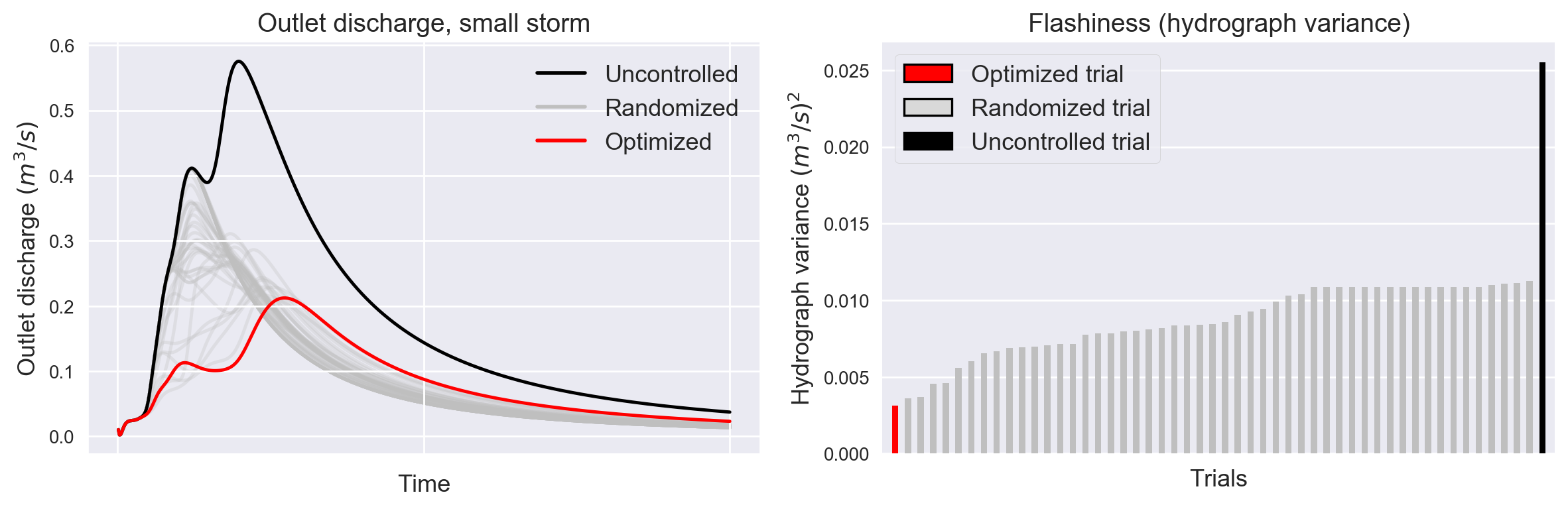
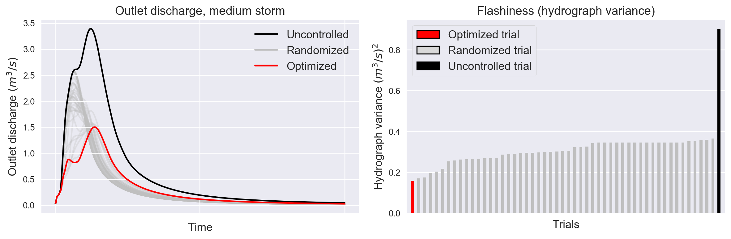
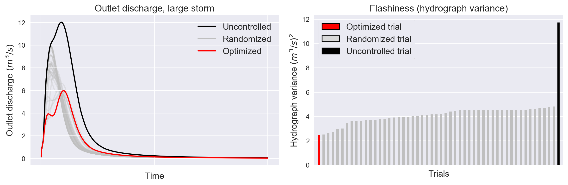
Figure S4: Left: simulated hydrographs for the uncontrolled scenario (black), naive controller placement (gray), and the optimized controller placement (red) under small, medium and large storm events (top to bottom). Right: flashiness (as measured by the variance of the hydrograph) for each simulation.

S6 Peak discharge for storm events of different sizes

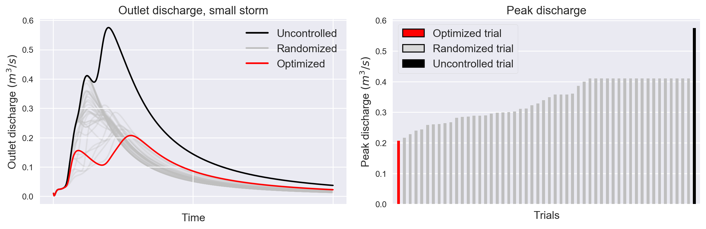
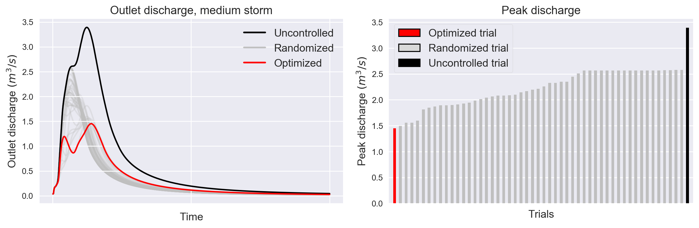
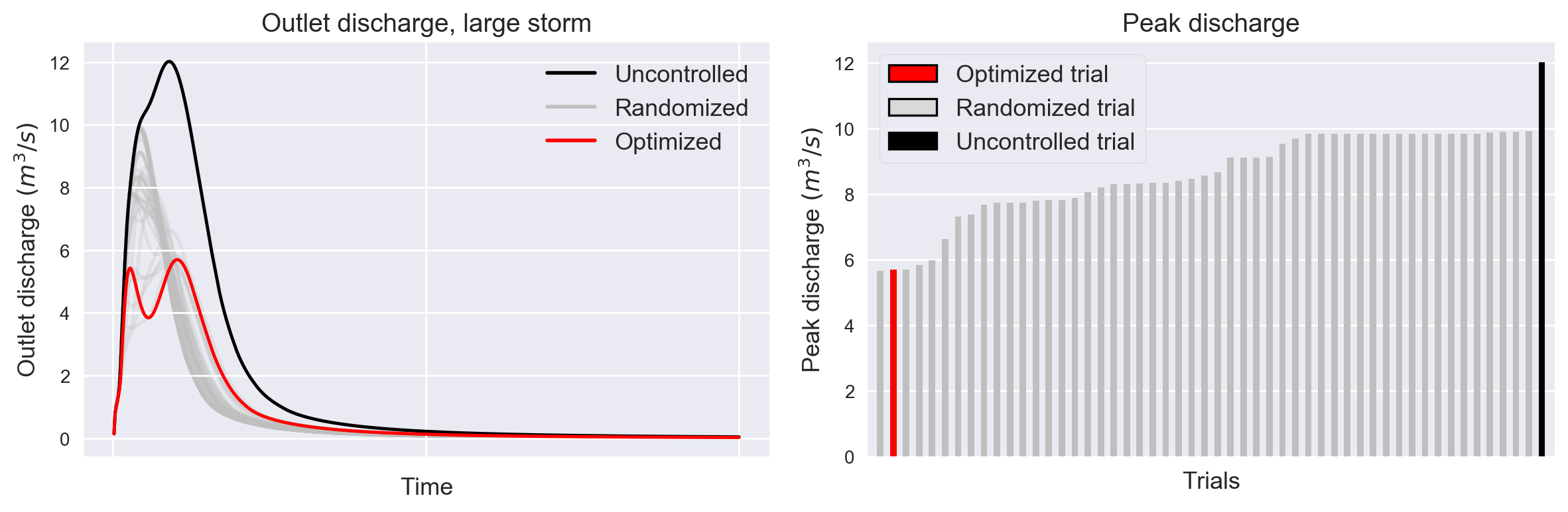
Figure S5: Left: simulated hydrographs for the uncontrolled scenario (black), naive controller placement (gray), and the optimized controller placement (red) under small, medium and large storm events (top to bottom). Right: peak discharge for each simulation.

S7 Hydrograph variance for all simulations

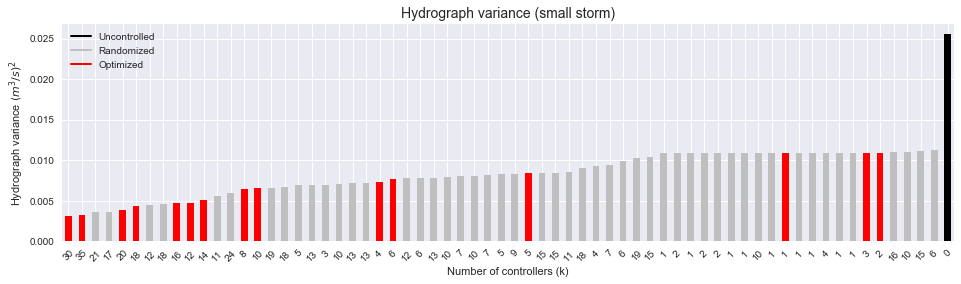
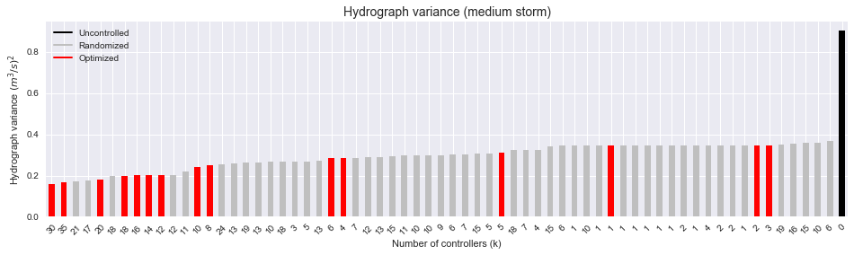
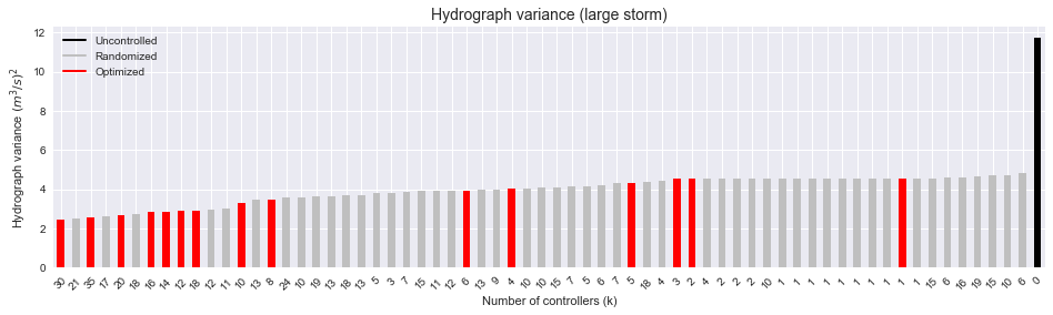
Figure S6: Hydrograph variance for small, medium and large storms under all model runs.

S8 Peak discharge for all simulations

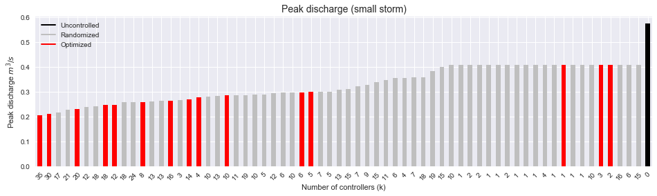
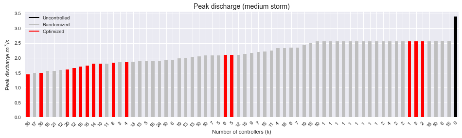
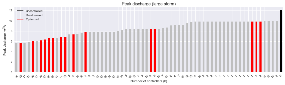
Figure S7: Peak discharge for small, medium and large storms under all model runs.

S9 Performance metrics by number of controllers

References

- [1] B. Kerkez, C. Gruden, M. Lewis, L. Montestruque, M. Quigley, B. Wong, A. Bedig, R. Kertesz, T. Braun, O. Cadwalader, A. Poresky, C. Pak, Smarter stormwater systems, Environmental Science & Technology 50 (14) (2016) 7267–7273. doi:10.1021/acs.est.5b05870.
- [2] S. Doocy, A. Daniels, S. Murray, T. D. Kirsch, The human impact of floods: a historical review of events 1980-2009 and systematic literature review, PLoS Currents. doi:10.1371/currents.dis.f4deb457904936b07c09daa98ee8171a.
- [3] J. Wright, D. Marchese, Briefing: Continuous monitoring and adaptive control: the ‘smart’ storm water management solution, Proceedings of the Institution of Civil Engineers - Smart Infrastructure and Construction 170 (4) (2017) 86–89. doi:10.1680/jsmic.17.00017.
- [4] C. J. Walsh, A. H. Roy, J. W. Feminella, P. D. Cottingham, P. M. Groffman, R. P. Morgan, The urban stream syndrome: current knowledge and the search for a cure, Journal of the North American Benthological Society 24 (3) (2005) 706–723. doi:10.1899/04-028.1.
- [5] D. B. Booth, C. R. Jackson, Urbanization of aquatic systems: degradation thresholds, stormwater detection, and the limits of mitigation, Journal of the American Water Resources Association 33 (5) (1997) 1077–1090. doi:10.1111/j.1752-1688.1997.tb04126.x.
- [6] J. K. Finkenbine, J. Atwater, D. Mavinic, Stream health after urbanization, Journal of the American Water Resources Association 36 (5) (2000) 1149–1160.
- [7] L. Wang, J. Lyons, P. Kanehl, R. Bannerman, Impacts of urbanization on stream habitat and fish across multiple spatial scales, Environmental Management 28 (2) (2001) 255–266. doi:10.1007/s0026702409.
- [8] L. Sahagun, High cost of fighting urban runoff examined in report, LA Times.
- [9] M. Wines, Behind toledo’s water crisis, a long-troubled Lake Erie, New York Times 4.
- [10] E. A. Rosenberg, P. W. Keys, D. B. Booth, D. Hartley, J. Burkey, A. C. Steinemann, D. P. Lettenmaier, Precipitation extremes and the impacts of climate change on stormwater infrastructure in washington state, Climatic Change 102 (1-2) (2010) 319–349. doi:10.1007/s10584-010-9847-0.
- [11] Dams and Development: A New Framework for Decision-making - The Report of the World Commission on Dams, Routledge, 2000. doi:10.4324/9781315541518.
- [12] M. Arora, H. Malano, B. Davidson, R. Nelson, B. George, Interactions between centralized and decentralized water systems in urban context: A review, Wiley Interdisciplinary Reviews: Water 2 (6) (2015) 623–634. doi:10.1002/wat2.1099.
- [13] R. J. Hawley, G. J. Vietz, Addressing the urban stream disturbance regime, Freshwater Science 35 (1) (2016) 278–292. doi:10.1086/684647.
- [14] L. S. Coffman, R. Goo, R. Frederick, Low-impact development: An innovative alternative approach to stormwater management, in: WRPMD 1999, American Society of Civil Engineers, 1999. doi:10.1061/40430(1999)118.
- [15] E. Strecker, M. M. Quigley, B. R. Urbonas, J. Jones, J. Clary, Determining urban stormwater BMP effectiveness, Proceedings of the Water Environment Federation 2000 (6) (2000) 2395–2412. doi:10.2175/193864700785150457.
- [16] A. Askarizadeh, M. A. Rippy, T. D. Fletcher, D. L. Feldman, J. Peng, P. Bowler, A. S. Mehring, B. K. Winfrey, J. A. Vrugt, A. AghaKouchak, S. C. Jiang, B. F. Sanders, L. A. Levin, S. Taylor, S. B. Grant, From rain tanks to catchments: Use of low-impact development to address hydrologic symptoms of the urban stream syndrome, Environmental Science & Technology 49 (19) (2015) 11264–11280. doi:10.1021/acs.est.5b01635.
- [17] M. Bartos, B. Wong, B. Kerkez, Open storm: a complete framework for sensing and control of urban watersheds, Environmental Science: Water Research & Technology 4 (3) (2018) 346–358. doi:10.1039/c7ew00374a.
- [18] A. Mullapudi, B. P. Wong, B. Kerkez, Emerging investigators series: building a theory for smart stormwater systems, Environ. Sci.: Water Res. Technol. 3 (1) (2017) 66–77. doi:10.1039/c6ew00211k.
- [19] A. Mullapudi, M. Bartos, B. Wong, B. Kerkez, Shaping streamflow using a real-time stormwater control network, Sensors 18 (7) (2018) 2259. doi:10.3390/s18072259.
- [20] L. Montestruque, M. D. Lemmon, Globally coordinated distributed storm water management system, in: Proceedings of the 1st ACM International Workshop on Cyber-Physical Systems for Smart Water Networks - CySWater 2015, ACM Press, 2015. doi:10.1145/2738935.2738948.
- [21] C. H. Emerson, C. Welty, R. G. Traver, Watershed-scale evaluation of a system of storm water detention basins, Journal of Hydrologic Engineering 10 (3) (2005) 237–242. doi:10.1061/(asce)1084-0699(2005)10:3(237).
- [22] G. Petrucci, E. Rioust, J.-F. Deroubaix, B. Tassin, Do stormwater source control policies deliver the right hydrologic outcomes?, Journal of Hydrology 485 (2013) 188–200. doi:10.1016/j.jhydrol.2012.06.018.
- [23] B. P. Wong, B. Kerkez, Real-time control of urban headwater catchments through linear feedback: performance, analysis and site selection, Water Resources Research. doi:10.1029/2018wr022657.
- [24] M. S. Gelormino, N. L. Ricker, Model-predictive control of a combined sewer system, International Journal of Control 59 (3) (1994) 793–816. doi:10.1080/00207179408923105.
- [25] A. L. Mollerup, P. S. Mikkelsen, D. Thornberg, G. Sin, Controlling sewer systems - a critical review based on systems in three EU cities, Urban Water Journal 14 (4) (2016) 435–442. doi:10.1080/1573062x.2016.1148183.
- [26] M. J. Kirkby, Tests of the random network model, and its application to basin hydrology, Earth Surface Processes 1 (3) (1976) 197–212. doi:10.1002/esp.3290010302.
- [27] V. K. Gupta, E. Waymire, I. Rodríguez-Iturbe, On scales, gravity and network structure in basin runoff, in: Scale Problems in Hydrology, Springer Netherlands, 1986, pp. 159–184. doi:10.1007/978-94-009-4678-1_8.
- [28] V. K. Gupta, O. J. Mesa, Runoff generation and hydrologic response via channel network geomorphology — recent progress and open problems, Journal of Hydrology 102 (1-4) (1988) 3–28. doi:10.1016/0022-1694(88)90089-3.
- [29] O. J. Mesa, E. R. Mifflin, On the relative role of hillslope and network geometry in hydrologic response, in: Scale Problems in Hydrology, Springer Netherlands, 1986, pp. 1–17. doi:10.1007/978-94-009-4678-1_1.
- [30] A. Marani, R. Rigon, A. Rinaldo, A note on fractal channel networks, Water Resources Research 27 (12) (1991) 3041–3049. doi:10.1029/91wr02077.
- [31] B. M. Troutman, M. R. Karlinger, Unit hydrograph approximations assuming linear flow through topologically random channel networks, Water Resources Research 21 (5) (1985) 743–754. doi:10.1029/wr021i005p00743.
- [32] R. Mantilla, V. K. Gupta, B. M. Troutman, Scaling of peak flows with constant flow velocity in random self-similar networks, Nonlinear Processes in Geophysics 18 (4) (2011) 489–502. doi:10.5194/npg-18-489-2011.
- [33] A. Tejedor, A. Longjas, I. Zaliapin, E. Foufoula-Georgiou, Delta channel networks: 1. a graph-theoretic approach for studying connectivity and steady state transport on deltaic surfaces, Water Resources Research 51 (6) (2015) 3998–4018. doi:10.1002/2014wr016577.
- [34] A. Tejedor, A. Longjas, I. Zaliapin, E. Foufoula-Georgiou, Delta channel networks: 2. metrics of topologic and dynamic complexity for delta comparison, physical inference, and vulnerability assessment, Water Resources Research 51 (6) (2015) 4019–4045. doi:10.1002/2014wr016604.
- [35] M. Zellner, D. Massey, E. Minor, M. Gonzalez-Meler, Exploring the effects of green infrastructure placement on neighborhood-level flooding via spatially explicit simulations, Computers, Environment and Urban Systems 59 (2016) 116 – 128. doi:10.1016/j.compenvurbsys.2016.04.008.
- [36] J. E. Schubert, M. J. Burns, T. D. Fletcher, B. F. Sanders, A framework for the case-specific assessment of green infrastructure in mitigating urban flood hazards, Advances in Water Resources 108 (2017) 55 – 68. doi:10.1016/j.advwatres.2017.07.009.
- [37] L. Yao, L. Chen, W. Wei, R. Sun, Potential reduction in urban runoff by green spaces in beijing: A scenario analysis, Urban Forestry & Urban Greening 14 (2) (2015) 300 – 308. doi:10.1016/j.ufug.2015.02.014.
- [38] B. Zhang, G. di Xie, N. Li, S. Wang, Effect of urban green space changes on the role of rainwater runoff reduction in beijing, china, Landscape and Urban Planning 140 (2015) 8 – 16. doi:10.1016/j.landurbplan.2015.03.014.
- [39] B. A. Norton, A. M. Coutts, S. J. Livesley, R. J. Harris, A. M. Hunter, N. S. Williams, Planning for cooler cities: A framework to prioritise green infrastructure to mitigate high temperatures in urban landscapes, Landscape and Urban Planning 134 (2015) 127 – 138. doi:10.1016/j.landurbplan.2014.10.018.
- [40] S. Meerow, J. P. Newell, Spatial planning for multifunctional green infrastructure: Growing resilience in detroit, Landscape and Urban Planning 159 (2017) 62 – 75. doi:10.1016/j.landurbplan.2016.10.005.
- [41] J. Schilling, J. Logan, Greening the rust belt: A green infrastructure model for right sizing america’s shrinking cities, Journal of the American Planning Association 74 (4) (2008) 451–466.
- [42] M. Cattafi, M. Gavanelli, M. Nonato, S. Alvisi, M. Franchini, Optimal placement of valves in a water distribution network with clp(fd), Theory and Practice of Logic Programming 11 (4-5) (2011) 731–747. doi:10.1017/S1471068411000275.
- [43] E. Creaco, M. Franchini, S. Alvisi, Optimal placement of isolation valves in water distribution systems based on valve cost and weighted average demand shortfall, Water Resources Management 24 (15) (2010) 4317–4338. doi:10.1007/s11269-010-9661-5.
- [44] L. Perelman, A. Ostfeld, Application of graph theory to sensor placement in water distribution systems, in: World Environmental and Water Resources Congress 2013, American Society of Civil Engineers, 2013. doi:10.1061/9780784412947.060.
- [45] A. Yazdani, P. Jeffrey, Robustness and vulnerability analysis of water distribution networks using graph theoretic and complex network principles, in: Water Distribution Systems Analysis 2010, American Society of Civil Engineers, 2011. doi:10.1061/41203(425)85.
- [46] V. G. Tzatchkov, V. H. Alcocer-Yamanaka, V. B. Ortíz, Graph theory based algorithms for water distribution network sectorization projects, in: Water Distribution Systems Analysis Symposium 2006, American Society of Civil Engineers, 2008. doi:10.1061/40941(247)172.
- [47] S. Hajebi, E. Roshani, N. Cardozo, S. Barrett, A. Clarke, S. Clarke, Water distribution network sectorisation using graph theory and many-objective optimisation, Journal of Hydroinformatics. doi:10.2166/hydro.2015.144.
- [48] Y.-Y. Liu, A.-L. Barabási, Control principles of complex systems, Reviews of Modern Physics 88 (3). doi:10.1103/revmodphys.88.035006.
- [49] Y.-Y. Liu, J.-J. Slotine, A.-L. Barabási, Controllability of complex networks, Nature 473 (7346) (2011) 167–173. doi:10.1038/nature10011.
- [50] J. Ruths, D. Ruths, Control profiles of complex networks, Science 343 (6177) (2014) 1373–1376. doi:10.1126/science.1242063.
- [51] T. H. Summers, J. Lygeros, Optimal sensor and actuator placement in complex dynamical networks, IFAC Proceedings Volumes 47 (3) (2014) 3784–3789. doi:10.3182/20140824-6-za-1003.00226.
- [52] G. Yan, J. Ren, Y.-C. Lai, C.-H. Lai, B. Li, Controlling complex networks: How much energy is needed?, Physical Review Letters 108 (21). doi:10.1103/physrevlett.108.218703.
- [53] G. Yan, G. Tsekenis, B. Barzel, J.-J. Slotine, Y.-Y. Liu, A.-L. Barabási, Spectrum of controlling and observing complex networks, Nature Physics 11 (9) (2015) 779–786. doi:10.1038/nphys3422.
- [54] A. Shirin, I. S. Klickstein, F. Sorrentino, Optimal control of complex networks: Balancing accuracy and energy of the control action, Chaos: An Interdisciplinary Journal of Nonlinear Science 27 (4) (2017) 041103. doi:10.1063/1.4979647.
- [55] J. F. OCallaghan, D. M. Mark, The extraction of drainage networks from digital elevation data, Computer Vision, Graphics, and Image Processing 27 (2) (1984) 247. doi:10.1016/s0734-189x(84)80047-x.
- [56] D. G. Tarboton, A new method for the determination of flow directions and upslope areas in grid digital elevation models, Water Resources Research 33 (2) (1997) 309–319. doi:10.1029/96wr03137.
- [57] R. L. Shreve, Stream lengths and basin areas in topologically random channel networks, The Journal of Geology 77 (4) (1969) 397–414. doi:10.1086/628366.
- [58] I. Rodriguez-Iturbe, A. Rinaldo, Fractal river basins: chance and self-organization, Cambridge University Press, 2001.
- [59] L. D. Tak, R. L. Bras, Incorporating hillslope effects into the geomorphologic instantaneous unit hydrograph, Water Resources Research 26 (10) (1990) 2393–2400.
- [60] I. D. Moore, R. Grayson, A. Ladson, Digital terrain modelling: a review of hydrological, geomorphological, and biological applications, Hydrological processes 5 (1) (1991) 3–30.
- [61] M. Bartos, Controller placement code, https://github.com/kLabUM/hydraulic-controller-placement (2018).
- [62] M. Bartos, pysheds: simple and fast watershed delineation in python, https://github.com/mdbartos/pysheds (2018).
- [63] B. Lehner, K. Verdin, A. Jarvis, New global hydrography derived from spaceborne elevation data, Eos, Transactions American Geophysical Union 89 (10) (2008) 93. doi:10.1029/2008eo100001.
- [64] United States Geological Survey, National hydrography geodatabase, https://viewer.nationalmap.gov/viewer/nhd.html?p=nhd (2013).
- [65] L. Mays, Water Resources Engineering, John Wiley & Sons, 2010.
- [66] J. A. Moody, B. M. Troutman, Characterization of the spatial variability of channel morphology, Earth Surface Processes and Landforms 27 (12) (2002) 1251–1266. doi:10.1002/esp.403.
- [67] United States Environmental Protection Agency, ORD stormwater management model, https://github.com/USEPA/Stormwater-Management-Model (2018).
- [68] B. P. Wong, B. Kerkez, Adaptive measurements of urban runoff quality, Water Resources Research 52 (11) (2016) 8986–9000. doi:10.1002/2015WR018013.
- [69] D. Muschalla, B. Vallet, F. Anctil, P. Lessard, G. Pelletier, P. A. Vanrolleghem, Ecohydraulic-driven real-time control of stormwater basins, Journal of Hydrology 511 (2014) 82–91. doi:10.1016/j.jhydrol.2014.01.002.
- [70] A. Poresky, R. Boyle, O. Cadwalader, Piloting real time control retrofits of stormwater facilities: Two oregon case studies and beyond, Proceedings of the Pacific Northwest Clean Water Association, Boise, ID, USA (2015) 26–27.