Statistical periodicity in driven quantum systems: General formalism and application to noisy Floquet topological chains

Abstract

Much recent experimental effort has focused on the realization of exotic quantum states and dynamics predicted to occur in periodically driven systems. But how robust are the sought-after features, such as Floquet topological surface states, against unavoidable imperfections in the periodic driving? In this work, we address this question in a broader context and study the dynamics of quantum systems subject to noise with periodically recurring statistics. We show that the stroboscopic time evolution of such systems is described by a noise-averaged Floquet superoperator. The eigenvectors and -values of this superoperator generalize the familiar concepts of Floquet states and quasienergies and allow us to describe decoherence due to noise efficiently. Applying the general formalism to the example of a noisy Floquet topological chain, we re-derive and corroborate our recent findings on the noise-induced decay of topologically protected end states. These results follow directly from an expansion of the end state in eigenvectors of the Floquet superoperator.

I Introduction

The periodic modulation of a quantum system is a powerful tool to engineer exotic, effectively static models. Even more intriguingly, it provides a pathway to realize novel phases of matter without time-independent counterparts. Central to these ideas is the existence of Floquet states that generalize the notion of eigenstates of a static Hamiltonian to the periodically driven setting Eckardt (2017). In the basis of Floquet states, the stroboscopic time evolution of a driven system resembles the undriven Hamiltonian dynamics, albeit described by an effective Hamiltonian Rahav et al. (2003a, b); Goldman and Dalibard (2014). In particular, a system that is initialized in a Floquet eigenstate, remains in this state. Floquet engineering, thus, amounts to designing an effective Hamiltonian such that its spectrum and eigenstates, i.e., the quasienergies and Floquet states, have the desired, e.g., topological Kitagawa et al. (2010); Rudner et al. (2013), properties.

A common feature of all such proposals is that a perfect periodicity of the driving is required for a well-defined effective Hamiltonian and Floquet eigenstates. This raises questions about the effects of imperfections in the driving protocol. In a recent paper Rieder et al. (2017), we addressed this question for the specific example of a Floquet topological chain with timing noise. For perfectly periodic driving, this system hosts topologically protected end states. Timing noise induces transitions between Floquet states and causes a particle that is initialized in such an end state to decay into the bulk. Interestingly, this decay is slowed down substantially if the bulk states are localized. The noise in this case can be treated as a perturbation to the perfectly periodic driving leading to dynamics captured by a discrete-time Floquet-Lindblad equation (FLE).

Here, we broaden the scope of this investigation. We show that the stroboscopic evolution of a driven system with stochastic periodicity, i.e., with random fluctuations that obey periodically recurring statistics, is described by a Floquet superoperator which directly generalizes the notion of a conventional Floquet operator. This description is not limited to weak noise and does not even rely on the existence of a perfectly periodic and noiseless limit. In this sense, it also applies to systems which are driven exclusively by noise. Within this formalism, we re-derive and corroborate the results for a noisy Floquet topological chain as reported in Ref. Rieder et al. (2017). Here, we obtain the decay of the end state by calculating the eigenoperators and eigenvalues of the noise-averaged Floquet superoperator.

The remainder of the paper is organized as follows: We begin in Sec. II by defining the notion of statistical periodicity that is underlying our work and we introduce key concepts such as the Floquet superoperator. The formalism to describe systems that are periodic on average is developed in Sec. III for the example of a Floquet system that is perturbed by timing noise. We show in Sec. IV how this approach captures fully random driving with temporally periodic statistics. Section V illustrates the theory by applying it to the noisy Floquet topological chain we studied previously in Ref. Rieder et al. (2017). Finally, we discuss our results and future directions in Sec. VI.

II Statistical periodicity

In this paper, we study the dynamics of quantum systems subject to stochastic driving protocols with periodically recurring statistics. More specifically, we focus on driving protocols which can be defined in terms of elementary driving cycles that are applied repeatedly, but with random and statistically independent parameter fluctuations from cycle to cycle. Since this definition is rather general, we find it worthwhile to briefly mention the perhaps simplest incarnation of such a driving protocol. In this simple example, an elementary cycle consists of applying a (constant) Hamiltonian $H_{1}$ for a duration of $T_{1}$ followed by the application of (another) Hamiltonian $H_{2}$ for a duration of $T_{2}$, where $T_{1}$ and $T_{2}$ are random and are drawn from the same distribution in each individual cycle. One of the central goals of this paper is to derive an evolution equation describing the noise-averaged dynamics of such systems.

To this end, we first consider the evolution under a specific realization of the stochastic drive, and we denote the quantum state of the system after $n$ elementary driving cycles by $\ket{\psi_{n}}$. The system’s evolution during one driving cycle is given by

$$\ket{\psi_{n+1}}=U_{{\rm F},n+1}\ket{\psi_{n}},$$ (1)

where the subscript F suggests that for deterministic driving, i.e., when $U_{{\rm F},n}=U_{\rm F}$ for all $n$, we recover a standard Floquet problem (if $U_{\rm F}$ is generated by a Hamiltonian with non-trivial time dependence). By taking the average over different realizations of the stochastic drive, which we indicate by an overbar hereafter, we obtain the density matrix $\rho_{n}=\overline{\ket{\psi_{n}}\bra{\psi_{n}}}$. Working with the density matrix instead of the noise-averaged pure state allows us to directly calculate physical observables as

$$\overline{\langle O_{n}\rangle}=\overline{\braket{\psi_{n}}{O}{\psi_{n}}}=\mathop{\mathrm{tr}}\!\left(O\overline{\ket{\psi_{n}}\bra{\psi_{n}}}\right)=\mathop{\mathrm{tr}}(O\rho_{n}).$$ (2)

The evolution equation for $\rho_{n}$ can be cast as a generalization of the familiar relation $\ket{\psi_{n+1}}=U_{\rm F}\ket{\psi_{n}}$ for noiseless Floquet systems, where $U_{\rm F}$ is the usual Floquet operator describing the time evolution over one period. To derive this evolution equation, we start by expressing $\rho_{n+1}$ as the average of Eq. (1),

$$\rho_{n+1}=\overline{\ket{\psi_{n+1}}\bra{\psi_{n+1}}}=\overline{U_{{\rm F},n+1}\ket{\psi_{n}}\bra{\psi_{n}}U_{{\rm F},n+1}^{\dagger}}.$$ (3)

Under the assumption of statistical independence of fluctuations which occur in different driving cycles, the average in the above expression factorizes and can be taken separately over $U_{\mathrm{F},n+1}$ and $\ket{\psi_{n}}$. We thus obtain

$$\rho_{n+1}=\overline{U_{{\rm F},n+1}\rho_{n}U_{{\rm F},n+1}^{\dagger}}=\mathcal{F}\rho_{n}.$$ (4)

This relation defines the noise-averaged Floquet superoperator $\mathcal{F}$. We note that while we introduce $\mathcal{F}$ to describe the dynamics of systems subject to stochastic driving, the concept of a Floquet superoperator also arises in periodically driven systems in the presence of (Markovian) dissipation Haake (2010). To illustrate the basic properties of the Floquet superoperator $\mathcal{F}$ it is useful to first consider the case of perfectly periodic driving described by a Floquet operator $U_{\rm F}$ such that $\mathcal{F}=\mathcal{U}_{\rm F}$ and

$$\rho_{n+1}=\mathcal{U}_{\rm F}\rho_{n}=U_{\rm F}\rho_{n}U_{\rm F}^{\dagger}.$$ (5)

Then, the eigenvalues and eigenoperators of $\mathcal{U}_{\rm F}$ can be obtained immediately from an eigenbasis of the Floquet operator $U_{\rm F}$. For the states $\ket{\alpha}$ which satisfy $U_{\rm F}\ket{\alpha}=e^{-iT\varepsilon_{\alpha}}\ket{\alpha}$, where $T$ is the period of the drive and $\varepsilon_{\alpha}$ the quasienergy of the state $\ket{\alpha}$, we find

$$\mathcal{U}_{\rm F}(\ket{\alpha}\bra{\beta})=U_{\rm F}\ket{\alpha}\bra{\beta}U_{\rm F}^{\dagger}=e^{-iT\left(\varepsilon_{\alpha}-\varepsilon_{\beta}\right)}\ket{\alpha}\bra{\beta},$$ (6)

i.e., the eigenoperators of $\mathcal{U}_{\rm F}$ take the form $\ket{\alpha}\bra{\beta}$ and the corresponding eigenvalues are determined by the differences of quasienergies $\varepsilon_{\alpha}-\varepsilon_{\beta}$. Unitarity of the perfectly periodic dynamics guarantees that the eigenvalues of $\mathcal{U}_{\rm F}$ have unit modulus. This does not apply if the dynamics is generated by a stochastic driving protocol. For instance, timing noise as considered in Ref. Rieder et al. (2017) and Sec. III.1 below induces transitions between the Floquet states $\ket{\alpha}$, causing the system to eventually heat up to infinite temperature, i.e., for $n\to\infty$ the state becomes fully mixed, $\rho_{n}\to\mathbbm{1}/D$, where $D$ is the dimension of the Hilbert space. In the spectrum of $\mathcal{F}$, this is reflected in $\mathbbm{1}$ being the unique eigenoperator corresponding to the eigenvalue $1$, i.e., $\mathcal{F}\mathbbm{1}=\mathbbm{1}$. Writing the eigenvalues of $\mathcal{F}$ as $e^{-i\lambda}$, noise-induced decoherence implies that all “eigenphases” $\lambda\neq 0$ corresponding to non-stationary states acquire finite imaginary parts $\mathop{\mathrm{Im}}(\lambda)<0$. Thus, the spectrum of $\mathcal{F}$ reveals that at long times noisy Floquet systems generically heat up to a featureless infinite-temperature state, but remnants of the properties of the system for perfectly periodic driving can survive in the dynamics. The latter can also be described efficiently by expanding the system’s state in eigenoperators of $\mathcal{F}$. We pursue this strategy for the example of a noisy Floquet topological chain in Sec. V. First, however, we derive formal expressions for the Floquet superoperator for noisy Floquet systems and for systems which are subject to purely random driving in Secs. III and IV, respectively.

III Noisy Floquet systems

To connect to the familiar physics and concepts of periodically driven (Floquet) systems, we first introduce stochastic driving as a perturbation. That is, we consider a slight imperfection causing random fluctuations around a periodic driving protocol. Motivated by much recent work on Floquet systems, we consider piecewise constant driving, i.e., the time-dependence of the Hamiltonian is a succession of sudden quenches interluded by phases during which the Hamiltonian is kept constant. Moreover, to not burden the discussion with unnecessary complications, we develop the formalism for the simplest case of binary driving that is defined in terms of just two Hamiltonians $H_{1,2}$ which are alternated. The generalization of our considerations to a driving protocol that comprises more than two steps is straightforward and summarized in Sec. III.3.

III.1 Timing noise

Our starting point is a perfectly periodic driving protocol described by the Hamiltonian

$$H(t)=\begin{cases}H_{1},&nT\leq t<nT+T_{1},\\ H_{2},&nT+T_{1}\leq t<\left(n+1\right)T,\end{cases}$$ (7)

i.e., $H(t)=H_{1}$ is kept constant for a time span of length $T_{1}$, and then switched to $H_{2}$ which is applied for $T_{2}$. The cycle of duration $T=T_{1}+T_{2}$ is then repeated periodically, and the integer $n$ counts the number of elapsed driving cycles. The evolution of the system during one driving period is described by the Floquet operator $U_{\rm F}$, which is given by

$$U_{\rm F}=\mathsf{T}e^{-i\int_{0}^{T}dt\,H(t)}=U_{2}U_{1}=e^{-iT_{2}H_{2}}e^{-iT_{1}H_{1}},$$ (8)

where $\mathsf{T}$ denotes time ordering. A special case of this driving protocol arises in the limit when $H_{2}$ is applied as a short pulse of strength $\lambda$ and duration $T_{2}\to 0$. This limit defines the class of periodically “kicked” systems with time-dependent Hamiltonian

$$H(t)=H_{1}+\lambda\sum_{n\in\mathbbm{N}}\delta(t-nT)H_{2},$$ (9)

giving rise to a Floquet operator of the form $U_{\rm F}=e^{-i\lambda H_{2}}e^{-iTH_{1}}$. The Floquet operator determines the stroboscopic time evolution of the state of the system: At multiples of the driving period $T$, the system’s state is given by $\ket{\psi_{n}}=\ket{\psi(nT)}=U_{\rm F}^{n}\ket{\psi_{0}}$ for the initial state $\ket{\psi_{0}}$. By diagonalizing $U_{\rm F}\ket{\alpha}=e^{-iT\varepsilon_{\alpha}}\ket{\alpha}$, we can thus describe the system in terms of its Floquet eigenstates $\ket{\alpha}$ and their associated quasienergies $\varepsilon_{\alpha}$.

The ideal scenario of perfectly periodic driving outlined thus far—and extensions to more elaborate driving schemes—form the basis of a great number of proposals to design Floquet quantum matter. In any realistic experimental implementation, however, noise and imperfections cannot be eliminated completely. A case in point are experiments that demonstrate Floquet topological insulators in photonic waveguides Mukherjee et al. (2017); Maczewsky et al. (2017), where time evolution of a quantum system is emulated by the propagation of light in the waveguide Longhi (2009); Szameit and Nolte (2010). Consequently, fabrication defects in the waveguide amount to timing noise in the emulated quantum dynamics. A simple model for this type of noise replaces the duration $T_{i}$ for which the Hamiltonian $H_{i}$ in Eq. (7) is applied during the $n$th driving cycle by $T_{in}=T_{i}+\tau_{in}$. Noise in $T_{in}$ is incorporated in the random number $\tau_{in}$, which has vanishing mean, $\overline{\tau_{in}}=0$ and fluctuations given by $\overline{\tau_{in}^{2}}=\tau^{2}$. Further, we assume that the time shifts in different parts of a single cycle as well as in different cycles are uncorrelated, i.e., $\overline{\tau_{in}\tau_{jn^{\prime}}}=\tau^{2}\delta_{ij}\delta_{nn^{\prime}}$. This assumption is reasonable in experiments in which the binary driving is realized by sudden quenches of the Hamiltonian parameters that suffer from imperfections. The time-dependent Hamiltonian is then given by

$$H(t)=\begin{cases}H_{1},&t_{n}\leq t<t_{n}+T_{1n},\\ H_{2},&t_{n}+T_{1n}\leq t<t_{n}+T_{1n}+T_{2n}.\end{cases}$$ (10)

In this expression, $t_{n}$ is the elapsed time after a particular realization of $n$ noisy driving cycles. The value of $t_{n}$ depends on all prior time shifts:

$$t_{n}=\sum_{n^{\prime}=1}^{n}\sum_{i=1,2}T_{in^{\prime}}=nT+\sum_{n^{\prime}=1}^{n}\sum_{i=1,2}\tau_{in^{\prime}}.$$ (11)

Evidently, $t_{n}$ is itself a random variable. It’s mean $\overline{t_{n}}=nT+\sum_{n^{\prime}=1}^{n}\sum_{i=1,2}\overline{\tau_{in}}=nT$ coincides with the time span corresponding to $n$ noiseless driving periods, while the fluctuations of $t_{n}$ grow as $\sqrt{n}$. The state of the system after $n$ driving cycles is given by

$$\ket{\psi_{n}}=U_{{\rm F},n}\dotsb U_{{\rm F},1}\ket{\psi_{0}}.$$ (12)

Here, $U_{{\rm F},n}$ denotes a “noisy” Floquet operator. We obtain it from a straightforward generalization of Eq. (8),

$$U_{{\rm F},n}=\mathsf{T}e^{-i\int_{t_{n-1}}^{t_{n}}dt\,H(t)}=e^{-iT_{2n}H_{2}}e^{-iT_{1n}H_{1}}.$$ (13)

In full analogy, we can extend the kicking protocol defined by Eq. (9) to include timing noise Oskay et al. (2003); Bitter and Milner (2016, 2017); ČadeŽ et al. (2017); Cadez et al. (2018):

$$H(t)=H_{1}+\lambda\sum_{n}\delta(t-t_{n})H_{2}.$$ (14)

With $t_{n}$ defined as in Eq. (11), the waiting time between two consecutive kicks is given by $t_{n+1}-t_{n}=T+\tau_{1n}$. The resulting noisy kicking protocol is described by a Floquet operator that takes exactly the same form as the one for the binary Floquet system in Eq. (13) if in addition to timing noise we allow for fluctuations of the kicking strength, i.e., we replace $\lambda\to\lambda+\tau_{2n}$.

We have thus specified the noisy Floquet operator that determines the evolution of the system’s state $\ket{\psi_{n}}$ during one particular realization of a noisy driving cycle as given in Eq. (1). We now proceed to evaluate the average in Eq. (4) to obtain a formal expression for the Floquet superoperator $\mathcal{F}$.

III.2 Formal Solution

For a given distribution of the fluctuating times $T_{in}$ in Eq. (13), the average in Eq. (4) can be carried out explicitly. To begin with, we focus on the first step of the $n$th driving cycle. The time evolution of the density matrix during this step is given by

$$\rho_{n+1,1}=\overline{U_{n+1,1}\rho_{n}U_{n+1,1}^{\dagger}},$$ (15)

where $U_{n+1,1}=e^{-iT_{1n}H_{1}}$. In order to perform the noise average, we rewrite the time evolution in terms of the superoperator $\mathcal{H}_{1}$, which is defined by $\mathcal{H}_{1}A=[H_{1},A]$ for a (matrix) operator $A$. Equation (15) can now be recast as

$$\rho_{n+1,1}=\overline{e^{-iT_{1n}\mathcal{H}_{1}}}\rho_{n}.$$ (16)

A way to see the equivalence of Eqs. (15) and (16) which proves useful in the following, is to note that as is the case for operators $A$ acting on pure states $\ket{\psi}$, functions of superoperators such as $\mathcal{H}_{1}$ can be written in terms of their spectral representation: From an eigenbasis $\ket{\alpha}$ of $H_{1}$ with $H_{1}\ket{\alpha}=E_{\alpha}\ket{\alpha}$ we obtain the eigenoperators $\ket{\alpha}\bra{\beta}$ of $\mathcal{H}_{1}$ which obey $\mathcal{H}_{1}(\ket{\alpha}\bra{\beta})=\left(E_{\alpha}-E_{\beta}\right)\ket{\alpha}\bra{\beta}$. Thus, the spectral representation of $\mathcal{H}_{1}$ reads

$$\mathcal{H}_{1}=\sum_{\alpha,\beta}\left(E_{\alpha}-E_{\beta}\right)\mathcal{P}_{\alpha\beta},$$ (17)

with the superoperator $\mathcal{P}_{\alpha\beta}$ defined by the relation $\mathcal{P}_{\alpha\beta}A=\ket{\alpha}\bra{\beta}\braket{\alpha}{A}{\beta}$. Analogously we obtain

$$e^{-iT_{1n}\mathcal{H}_{1}}\rho_{n}=\sum_{\alpha,\beta}e^{-iT_{1n}\left(E_{\alpha}-E_{\beta}\right)}\ket{\alpha}\bra{\beta}\braket{\alpha}{\rho_{n}}{\beta},$$ (18)

see Eq. (6). This expression can be seen to be equal to $U_{n+1,1}\rho_{n}U_{n+1,1}^{\dagger}$ by inserting the completeness relation of the states $\ket{\alpha}$ twice in the latter expression. While this shows how calculations with superoperators can be carried out analytically, the concrete implementation of the superoperator formalism for numerical purposes is discussed in Appendix A.

Returning to the average in Eq. (16), we note that its result depends on the distribution of the duration $T_{1n}$. For noisy Floquet systems, the average factorizes as $\overline{e^{-iT_{1n}\mathcal{H}_{1}}}=e^{-iT_{1}\mathcal{H}_{1}}\overline{e^{-i\tau_{n1}\mathcal{H}_{1}}}.$ Exemplary distributions for timing noise are a normal distribution with width $\tau$ and a uniform distribution on the interval $[-\sqrt{3}\tau,\sqrt{3}\tau]$, both leading to fluctuations $\overline{\tau_{n1}^{2}}=\tau^{2}$. We thus obtain

$$\mathcal{E}_{1}=\overline{e^{-i\tau_{n1}\mathcal{H}_{1}}}=\begin{cases}e^{-\tau^{2}\mathcal{H}_{1}^{2}/2},&\text{normal,}\\ \mathop{\mathrm{sinc}}(\sqrt{3}\tau\mathcal{H}_{1}),&\text{uniform,}\end{cases}$$ (19)

where $\mathop{\mathrm{sinc}}(x)=\sin(x)/x$ and we set $\mathop{\mathrm{sinc}}(0)=1$. Using the spectral representation Eq. (17) for the example of a uniform distribution of timing errors we thus obtain

$$\mathcal{E}_{1}=\sum_{\alpha,\beta}\mathop{\mathrm{sinc}}(\sqrt{3}\tau\left(E_{\alpha}-E_{\beta}\right))\mathcal{P}_{\alpha\beta}.$$ (20)

For any distribution of timing errors the full evolution during the first step can be written as

$$\rho_{n+1,1}=e^{-iT_{1}\mathcal{H}_{1}}\mathcal{E}_{1}\rho_{n}=\mathcal{U}_{1}\mathcal{E}_{1}\rho_{n}.$$ (21)

Repeating the above reasoning for the second step of the time evolution leads us to

$$\rho_{n+1}=\mathcal{F}\rho_{n}=\mathcal{U}_{2}\mathcal{E}_{2}\mathcal{U}_{1}\mathcal{E}_{1}\rho_{n},$$ (22)

where $\mathcal{E}_{2}$ is defined analogously to $\mathcal{E}_{1}$ in Eq. (19). As a consistency check, we note that for vanishing timing noise, i.e., $\tau\to 0$, from Eq. (19) we see that $\mathcal{E}_{i}=\mathbbm{1}$, and thus $\rho_{n+1}=\mathcal{U}_{\rm F}\rho_{n}$, where $\mathcal{U}_{\rm F}=\mathcal{U}_{2}\mathcal{U}_{1}=e^{-iT_{2}\mathcal{H}_{2}}e^{-iT_{1}\mathcal{H}_{1}}$. We now proceed to discuss the extension of the above derivation to multi-step piecewise constant driving protocols.

III.3 Extension to multi-step piecewise constant driving

Extended driving protocols, which are defined in terms of a sequence of Hamiltonians $H_{i}$ with $i=1,2,\dotsc,M$, can be treated in much the same way as the binary driving of the previous section. To be specific, if fluctuations of each of the $T_{in}$ are independent and obey the same statistics, we find

$$\rho_{n+1}=\mathcal{F}\rho_{n}=\mathcal{U}_{M}\mathcal{E}_{M}\dotsb\mathcal{U}_{1}\mathcal{E}_{1}\rho_{n},$$ (23)

where $\mathcal{U}_{i}=e^{-iT_{i}\mathcal{H}_{i}}$, and the $\mathcal{E}_{i}$ are defined as in Eq. (19). From this form it is straightforward to obtain a matrix representation of $\mathcal{F}$ by using the spectral representation of the superoperators $\mathcal{H}_{i}$ given in Eq. (17). Such a matrix representation can be used to find the eigenmodes and complex quasienergies of $\mathcal{F}$ numerically.

Alternatively, we can iterate the procedure of Sec. III.2 with one modification: A clear separation between the noiseless Floquet dynamics and the noise-induced dissipation can be established by commuting $\mathcal{U}_{1}$ in Eq. (22) through the noisy part of $\mathcal{E}_{2}$ of the second step. This can be done most easily before carrying out the noise average and by using the relation (here, again, for a binary driving protocol)

$$\begin{split}U_{{\rm F},n}&=U_{2}e^{-i\tau_{2n}H_{2}}U_{1}e^{-i\tau_{1n}H_{1}}\\ &=U_{\rm F}e^{-i\tau_{2n}U_{1}^{\dagger}H_{2}U_{1}}e^{-i\tau_{1n}H_{1}}.\end{split}$$ (24)

Extending this procedure to a driving protocol that consists of $M$ steps, we obtain

$$\rho_{n+1}=\mathcal{F}\rho_{n}=\mathcal{U}_{\rm F}\tilde{\mathcal{E}}_{M}\dotsb\tilde{\mathcal{E}}_{1}\rho_{n},$$ (25)

where now

$$\tilde{\mathcal{E}}_{i}=\begin{cases}e^{-\tau^{2}\mathcal{L}_{i}^{2}/2},&\text{normal,}\\ \mathop{\mathrm{sinc}}(\sqrt{3}\tau\mathcal{L}_{i}),&\text{uniform.}\end{cases}$$ (26)

The superoperators $\mathcal{L}_{i}$ act on operators $A$ according to $\mathcal{L}_{i}A=[L_{i},A]$, and the Hermitian operators $L_{i}$ are defined as

$$L_{i}=U_{1}^{\dagger}\dotsb U_{i-1}^{\dagger}H_{i}U_{i-1}\dotsb U_{1}.$$ (27)

The expression Eq. (25) for the Floquet superoperator is most convenient for studying a limiting case that is particularly relevant for experimental realizations of Floquet systems: weak timing noise.

III.4 Weak Noise: Discrete-Time Floquet-Lindblad Equation

As discussed in Sec. III.1, timing noise occurs in Floquet systems as a result of experimental imperfections. Therefore, it is often justified to treat noise as a weak perturbation. In particular, if the spectra of the Hamiltonians $H_{i}$ constituting the driving protocol are bounded by an energy scale $J$ (e.g., the single-particle bandwidth in a tight-binding model) which satisfies $\tau J\ll 1$, the error superoperators in Eq. (26) can be expanded as

$$\tilde{\mathcal{E}}_{i}=\mathbbm{1}-\frac{\tau^{2}}{2}\mathcal{L}_{i}^{2}.$$ (28)

We note that both normal and uniform distributions of time shifts lead to the same lowest-order expansion. Inserting this expansion in Eq. (25) and keeping only terms up to $O(\tau^{2})$, we recover the FLE of Ref. Rieder et al. (2017), namely

$$\rho_{n+1}=\mathcal{U}_{\rm F}\left(\mathbbm{1}+\tau^{2}\sum_{i=1}^{M}\mathcal{D}[L_{i}]\right)\rho_{n}.$$ (29)

Here – in reminiscence of the usual Markovian master equation in Lindblad form – we introduced the “dissipator” $\mathcal{D}[L_{i}]=-\mathcal{L}_{i}^{2}/2$ for “jump operators” $L_{i}$. The similarity becomes obvious when writing the double-commutator structure of Eq. (29) for Hermitian jump operators $L=L^{\dagger}$, namely

$$-\frac{1}{2}\mathcal{L}^{2}\rho=-\frac{1}{2}\left[L,\left[L,\rho\right]\right]=L\rho L-\frac{1}{2}\left\{L^{2},\rho\right\}=\mathcal{D}[L]\rho$$ (30)

where $\mathcal{L}\rho=[L,\rho]$. Markovian master equations in Lindblad form find widespread use in quantum optics, where the time-local form of the equation results from a separation of scales between the typical time scale of the system’s evolution and the much shorter coherence time of the bath which induces dissipation in the system. Similarly, the FLE (29) is local in driving cycles, i.e., the state of the system $\rho_{n+1}$ after $n+1$ cycles depends only on the state $\rho_{n}$ after $n$ cycles and not on $\rho_{n^{\prime}}$ with $n^{\prime}<n$. This is due to our assumption that fluctuations of the stochastic drive are uncorrelated between different driving cycles, which is analogous to the Markovian baths encountered in the quantum optics context Reimer et al. (2018). Finally, we note that while here we found the FLE equation in the limit of weak noise, it is not guaranteed that the generator of the Floquet superoperator is of Lindblad form Schnell et al. (2018).

IV Fully random driving

Having given a detailed account of Floquet systems with timing noise, we now turn to a physical situation whose relation to any form of periodicity is perhaps less obvious: a time-dependent system subject to random telegraph noise (RTN) Zoller et al. (1981); Hu et al. (2015); Cai et al. (2016). We show how randomly timed pulses can be treated as an extreme case within our Floquet superoperator formalism.

IV.1 Random telegraph noise

For $\tau\to 0$, the evolution of the pure state of the noisy Floquet system Eq. (1) considered in the previous section reduces to the familiar perfectly periodic Floquet form. Here, instead, we consider a system that is driven exclusively by noise. As an example, consider a time-dependent Hamiltonian $H(t)=H_{0}+\lambda(t)V$, in which the random process $\lambda(t)$ jumps between two values $\lambda_{1,2}$ (thus, $H(t)$ jumps between $H_{1,2}=H_{0}+\lambda_{1,2}V$) at a rate $\gamma$. Under these conditions, the waiting times between sudden quenches from $H_{1}$ to $H_{2}$ and back are indeed statistically independent and follow an exponential distribution

$$P(t)=\gamma e^{-\gamma t}.$$ (31)

The average duration of a driving cycle corresponding to starting with $H_{1}$ and waiting for the Hamiltonian to change to $H_{2}$ and back is thus $T=2/\gamma$. As above, the noise averaged evolution of the system’s density matrix is given by Eq. (4) with the noisy Floquet operator defined in Eq. (13), but with $T_{in}$ drawn from the same exponential distribution. However, in the present case there is no meaningful definition of noise strength and thus of a noiseless limit. In the limiting case $\gamma\to 0$ the Hamiltonian of the system is simply $H(t)=H_{1}$ up to arbitrarily long times, while for $\gamma\to\infty$ corresponding to fast switching between $H_{1}$ and $H_{2}$ we show below that the time evolution follows the average Hamiltonian $\overline{H}=(H_{1}+H_{2})/2$ with only slow dephasing.

The formal results of Sec. III.2 can be generalized to this case of RTN by using the exponential distribution for the timing noise, yielding now

$$\mathcal{E}_{1}=\overline{e^{-i\tau_{n1}\mathcal{H}_{1}}}=\frac{\gamma}{\gamma+i\mathcal{H}_{1}}.$$ (32)

and, with $T_{i}=0$, the “Floquet” step reduces to $\mathcal{U}_{1}=e^{-iT_{1}H_{1}}=\mathbbm{1}$.

IV.2 Fast switching

The evolution of a system driven by RTN is given by [cf. Eqs. (22) and (32)]

$$\rho_{n+1}=\frac{\gamma}{\gamma+i\mathcal{H}_{2}}\frac{\gamma}{\gamma+i\mathcal{H}_{1}}\rho_{n}.$$ (33)

For fast switching rates, when $\gamma$ is much larger than the spectral bandwidth of the Hamiltonians $H_{i}$, a leading-order expansion in $1/\gamma$ yields

$$\rho_{n+1}=\left[\mathbbm{1}-\frac{i}{\gamma}\left(\mathcal{H}_{1}+\mathcal{H}_{2}\right)\right]\rho_{n}=e^{-iT(\mathcal{H}_{1}+\mathcal{H}_{2})/2}\rho_{n},$$ (34)

where $T=2/\gamma$ is the average period, and the exponentiation is valid up to the same order in $1/\gamma$. Equation (34) describes coherent evolution with the average Hamiltonian $(H_{1}+H_{2})/2$. Noise-induced dissipation is suppressed at fast switching rates, and occurs only at higher orders in $1/\gamma$. This suppression of decoherence at high switching rates has also been found in a description of the RTN-driven dynamics using a generalized master equation for the marginal system density operator Zoller et al. (1981); Hu et al. (2015); Cai et al. (2016).

V Application to noisy Floquet topological chains

We now turn to a concrete application of the formalism of statistical periodicity in driven quantum systems. In our recent work Rieder et al. (2017), we used a Floquet-Lindblad equation to describe the loss of an end state in a noisy Floquet topological chain. Here, we re-derive these results using the Floquet superoperator formalism introduced above.

V.1 Model

We consider a periodically time-dependent system of non-interacting spinless fermions on a one-dimensional ladder, implemented by varying the hopping amplitudes between neighboring lattice sites. One period comprises four steps of equal duration $T/4$ during each of which the system parameters are held constant. The switches between the different phases happen instantaneously. This is described by the Hamiltonian

$$H(t)=H_{i}\quad\text{for}\quad\left(i-1\right)T/4\leq t<iT/4,$$ (35)

where the time is measured modulo the period $T$ and

$$H_{i}=-\sum_{\mu,\nu}J_{\mu\nu}^{i}\left(c_{\mu}^{\dagger}c^{\phantom{{\dagger}}}_{\nu}+\mathrm{H.c.}\right),$$ (36)

for steps $i=1,2,3,4$. The sum runs over a combined index for sites on the ladder, $\mu=(j,s)$, with $j=0,\dotsc,L$ labeling doublets of sites at the plaquettes of the ladder and $s=\pm$ denoting their sublattice index as illustrated in Fig. 1. The hopping amplitudes $J_{\mu\nu}^{i}$ are chosen to enable hopping along disconnected pairs of nearest-neighbor lattice sites. In particular, we set $J_{\mu\nu}^{i}=J$ for all active bonds $\{\mu,\nu\}_{i}$ of step $i$ and $J_{\mu\nu}^{i}=0$ otherwise. We define the driving protocol by setting the active bonds as

$$\begin{split}\{\mu,\nu\}_{1}&=\{(j,s),(j-s,-s)\}\\ \{\mu,\nu\}_{2}&=\{(j,s),(j-2s,-s)\}\\ \{\mu,\nu\}_{3}&=\{(\mu,\nu)\}_{1}\\ \{\mu,\nu\}_{4}&=\{(j,s),(j,-s)\}.\end{split}$$ (37)

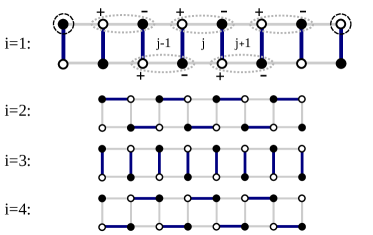
Figure 1: Sketch of the model considered in Sec. V. Lattice sites form doublets (gray dashed ellipses) and are labeled with the plaquette number $j$ and a doublet index $s=\pm$. The driving protocol comprises four steps $i=1,2,3,4$ during which hopping along only certain “active” bonds is allowed, as indicated with the thick blue lines. As a result of the particular driving, localized states, indicated by dashed black circles, form at the ends of the ladder at lattice sites $(0,-)$ and $(L,+)$.

At a special point in parameter space $J=2\pi/T$, which we call “resonant driving,” the eigenstates of the Floquet operator corresponding to the time-dependent Hamiltonian Eq. (35) can be understood intuitively: Each step of the driving protocol (of duration $T/4$) results in the full transfer of particles between two coupled neighboring sites, such that each particle accumulates a phase $\pi/2$. Therefore, during one period, a particle which is initialized on a single lattice site performs a full circle around a plaquette, thereby collecting a phase factor $2\pi$. The only exceptions to this behavior are particles initialized on one of the two lattice sites at the ends of the chain as indicated in Fig. 1. These skip two steps of the driving protocol, returning back to their original positions with a phase of $\pi$. We thus find a completely flat bulk band at quasienergy $0$ and two topologically protected Rieder et al. (2017) end states at quasienergy $\varepsilon T=\pi$. For a chain of length $L$, the left and right end states are $\ket{e_{l}}=\ket{0,-}$ and $\ket{e_{r}}=\ket{L,+}$. When we tune the system away from the point of resonant driving, the bulk band becomes dispersive, while the end states remain at quasienergy $\varepsilon T=\pi$, acquiring only a finite localization length.

The observation of these localized end states in an experimental realization would provide a clear signature of the non-trivial topological properties of the model. In Ref. Rieder et al. (2017), we studied how the observability of end states is affected by timing noise of the type described in Sec. III. Timing noise causes a particle which is initialized in an end state to decay into the system’s bulk. We showed that the nature of this decay depends critically on the nature of the bulk: For a delocalized bulk, noise-induced excitations out of the end state propagate away freely, resulting in an exponential decay with time. In contrast, when the bulk is localized these excitations “get stuck” and have a finite probability of returning to the end state. This results in a dramatically slowed-down diffusive decay. The different behaviors are shown in Fig. 2.

Figure 2: Survival probability of the end mode computed using Eq. (43) as a function of the number of noisy driving cycles, $n$. We use a ladder consisting of 50 rungs and a noise strength $\tau/T=1/80$. Away from the resonant driving point ($JT=5.8$, orange curve), $P_{\mathrm{s}}$ decays exponentially with $n$. The decay slows down to a diffusive one either when fine-tuning the system to $JT=2\pi$ (blue), or by including disorder ($VT/4=0.4$, yellow). The disordered curve is obtained by averaging over 80 simultaneous noise-disorder realizations, with error bars smaller than the line width. The solid black line shows an exponential decay with rate $2J^{2}\tau^{2}\simeq 0.0105$ as predicted in Eq. (52), the dotted line is a fit to a diffusive decay $\sim t^{-1/2}$, whereas the dashed line is the analytic result of Eq. (62).

To obtain localized bulk states in the Floquet ladder model, it is sufficient to consider the resonant driving point, $J=2\pi/T$, at which bulk states are dispersionless. In an experimental setting however, fine-tuning the system parameters to this point may be impractical, and a more accessible means of localizing bulk states is by adding quenched (time-independent) disorder to the system. To model the latter scenario, we consider random on-site disorder, adding to the Hamiltonian a term of the form

$$H_{\rm dis}=\sum_{\mu}V_{\mu}c^{\dagger}_{\mu}c^{\phantom{{\dagger}}}_{\mu},$$ (38)

where the potential $V_{\mu}$ is drawn randomly and independently for each lattice site of the ladder from the uniform distribution $[-V/2,V/2]$, with $V$ the disorder strength.

Note that on-site disorder destroys the topological protection of the boundary modes, since in the presence of a non-zero chemical potential they are allowed to shift away from the quasienergy zone boundary and hybridize with the bulk states. However, as shown in Ref. Rieder et al. (2017), for small values of the disorder strength $V$, end modes are still well separated from bulk states and localized at the boundaries of the system, such that studying their decay is a well defined problem.

In the following, we re-derive the results on the end state decay presented in Ref. Rieder et al. (2017) using the concepts and tools developed in the present paper.

V.2 Decay of the end state

We consider the stroboscopic time evolution of a particle that is initialized in the left end state $\ket{e}=\ket{e_{l}}$ of the chain, i.e., the initial density matrix is given by $\rho_{0}=\ket{e}\bra{e}$. The quantity of interest is the survival probability $P_{\mathrm{s}}$ of the end state which is defined as

$$P_{\mathrm{s}}=\overline{\left\lvert\braket{e}{\psi_{n}}\right\rvert^{2}}=\bra{e}\overline{\ket{\psi_{n}}\bra{\psi_{n}}}\ket{e}=\braket{e}{\rho_{n}}{e},$$ (39)

and is the probability to find a particle in the end state after $n$ driving cycles. In the absence of noise, $P_{\mathrm{s}}=1$ stays constant, while $P_{\mathrm{s}}$ decays over time for noisy driving. The dynamics of the system’s density is determined by the evolution Eq. (4), i.e., the time-evolved state is $\rho_{n}=\mathcal{F}^{n}\rho_{0}$. Before we specify the Floquet superoperator $\mathcal{F}$ for the noisy Floquet topological chain, we show how the survival probability can be evaluated in the superoperator formalism.

V.2.1 Survival probability from the Floquet superoperator

In the following, we find it convenient to adopt the terminology and notation of Ref. Zwolak and Vidal (2004). That is, we regard operators as “superkets” which we distinguish from normal kets (i.e., state vectors) by a subscript $\sharp$. To emphasize this interpretation, we write the density matrix as $\rho_{n}=\left\lvert\rho_{n}\right\rangle_{\sharp}$ and $\ket{e}\bra{e}=\left\lvert e\right\rangle_{\sharp}$ for the projector on the (left) end state of the topological chain to name two examples. A scalar product of superkets is given by $\braket{A}{B}_{\sharp}=\mathop{\mathrm{tr}}(A^{\dagger}B)$. Thence, the survival probability of the end state Eq. (39) can be written as an overlap of superkets:

$$P_{\mathrm{s}}=\mathop{\mathrm{tr}}(\ket{e}\bra{e}\overline{\ket{\psi_{n}}\bra{\psi_{n}}})=\braket{e}{\rho_{n}}_{\sharp},$$ (40)

where according to Eq. (4) the time-evolved density-matrix superket reads $\left\lvert\rho_{n}\right\rangle_{\sharp}=\mathcal{F}^{n}\left\lvert\rho_{0}\right\rangle_{\sharp}$. As in unitary Hamiltonian dynamics, a convenient representation of the time-evolved state and thus of the survival probability Eq. (40) can be given by expanding $\left\lvert\rho_{n}\right\rangle_{\sharp}$ in a basis of eigenoperators of $\mathcal{F}$. In particular, we denote the right eigenoperators of $\mathcal{F}$ by $\left\lvert\alpha\right\rangle_{\sharp}$,

$$\mathcal{F}\left\lvert\alpha\right\rangle_{\sharp}=e^{-i\lambda_{\alpha}}\left\lvert\alpha\right\rangle_{\sharp}.$$ (41)

Since, in general, the superoperator $\mathcal{F}$ is not normal, we have to distinguish its left and right eigenoperators. Denoting by $\prescript{}{\sharp}{\left\langle\alpha\right\rvert}$ the left eigenoperator corresponding to the eigenvalue $\lambda_{\alpha}$, the identity superoperator can be written as $\mathbbm{1}=\sum_{\alpha}\left\lvert\alpha\right\rangle_{\sharp}\!\bra{\alpha}$ (we use the symbol $\mathbbm{1}$ both for the identity operator and the identity superoperator). The stroboscopic time evolution can thus be written as

$$\left\lvert\rho_{n}\right\rangle_{\sharp}=\mathcal{F}^{n}\left\lvert\rho_{0}\right\rangle_{\sharp}=\sum_{\alpha}e^{-in\lambda_{\alpha}}\braket{\alpha}{\rho_{0}}_{\sharp}\left\lvert\alpha\right\rangle_{\sharp}.$$ (42)

Inserting this representation with $\left\lvert\rho_{0}\right\rangle_{\sharp}=\left\lvert e\right\rangle_{\sharp}$ in Eq. (40), the survival probability of the end state becomes

$$P_{\mathrm{s}}=\sum_{\alpha}e^{-in\lambda_{\alpha}}\left\lvert\braket{\alpha}{e}_{\sharp}\right\rvert^{2}.$$ (43)

$P_{\mathrm{s}}$ is evidently fully determined by the eigenoperators and eigenvalues of the Floquet superoperator $\mathcal{F}$. We proceed by specifying $\mathcal{F}$ for the noisy Floquet topological chain, and then evaluate the survival probability Eq. (43) for dispersive and localized bulk states, leading to exponential and diffusive decay, respectively, in Secs. V.2.3, V.2.4, and V.2.5.

V.2.2 Floquet superoperator for a noisy Floquet topological chain

The formal expression for the Floquet superoperator for the Floquet topological chain with timing noise is given by Eq. (23), where the coherent parts of the evolution, $\mathcal{U}_{i}=e^{-iT_{i}\mathcal{H}_{i}}$, are generated by the Hamiltonians $H_{i}$ in Eq. (36) (recall that $\mathcal{H}_{i}$ is defined by its action on an operator $A$, which is $\mathcal{H}_{i}A=[H_{i},A]$), and the error operators for normally distributed timing noise take the form given in Eq. (19), that is, the noise-averaged Floquet superoperator reads

$$\mathcal{F}=\mathcal{U}_{4}\mathcal{E}_{4}\dotsb\mathcal{U}_{1}\mathcal{E}_{1}=e^{-\frac{iT}{4}\mathcal{H}_{4}}e^{-\frac{\tau^{2}}{2}\mathcal{H}_{4}^{2}}\dotsb e^{-\frac{iT}{4}\mathcal{H}_{1}}e^{-\frac{\tau^{2}}{2}\mathcal{H}_{1}^{2}}.$$ (44)

To calculate the survival probability of the end state given in Eq. (43) we have to find the spectrum and the eigenoperators of $\mathcal{F}$. This can be done numerically as described further below, but close to resonant driving we can also make progress analytically. For this purpose, it is more convenient to work with the alternative representation of the Floquet superoperator given in Eq. (25), which in the present case becomes

$$\mathcal{F}=\mathcal{U}_{\rm F}e^{-\frac{\tau^{2}}{2}\mathcal{L}_{4}^{2}}e^{-\frac{\tau^{2}}{2}\mathcal{L}_{3}^{2}}e^{-\frac{\tau^{2}}{2}\mathcal{L}_{2}^{2}}e^{-\frac{\tau^{2}}{2}\mathcal{L}_{1}^{2}}.$$ (45)

The jump superoperators $\mathcal{L}_{i}$ are defined as $\mathcal{L}_{i}A=[L_{i},A]$, with the operators $L_{i}$ given in Eq. (27). At resonant driving, the latter take the form Rieder et al. (2017)

$$\begin{split}L_{1}&=J\sum_{j}\left(\ket{j,+}\bra{j-1,-}+\mathrm{H.c.}\right),\\ L_{2}&=J\sum_{j}\left(\ket{j,+}\bra{j,-}+\mathrm{H.c.}\right),\\ L_{3}&=J\sum_{j}\left(\ket{j,+}\bra{j+1,-}+\mathrm{H.c.}\right),\\ L_{4}&=J\sum_{j}\left(\ket{j,+}\bra{j,-}+\mathrm{H.c.}\right).\end{split}$$ (46)

This is the starting point of our analytical calculation of the end state’s decay close to resonant driving presented in the following. To extend the analysis beyond this limiting case, but also to include disorder in the model, it is necessary to determine the spectrum of the Floquet superoperator numerically. A matrix representation of $\mathcal{F}$ that is amenable to a numerical calculation of its eigenoperators and eigenvalues can be obtained by introducing a basis in the space of operators as described in App. A. All numerical results shown below are based on this representation.

V.2.3 Exponential decay for a dispersive bulk

We first consider the case of a dispersive bulk, in which the survival probability of the end state decays exponentially. Here, we show this analytically for a system that is close to but crucially slightly away from resonant driving, i.e., with $JT/4=\pi/2+\delta\phi$ where $\delta\phi\ll 1$. Then, the projector on the end state, $\left\lvert e\right\rangle_{\sharp}=\ket{e}\bra{e}$, is an approximate eigenstate of the Floquet superoperator with $\lambda_{e}=-i2\kappa^{2}$ where $\kappa=J\tau$, which according to Eq. (43) immediately implies the asserted exponential decay.

To obtain these results, we work in a basis of eigenoperators of the noiseless Floquet operator $\mathcal{U}_{\rm F}$. Starting from a basis of the Floquet operator $U_{\rm F}$ which consists of bulk states $\ket{b}$ and the left end state $\ket{e}$ (we disregard the right end state assuming that the system size is much larger than the localization length of the end states), a basis of $\mathcal{U}_{\rm F}$ is formed by the superkets $\left\lvert b;b^{\prime}\right\rangle_{\sharp}=\ket{b}\bra{b^{\prime}}$, $\left\lvert b;e\right\rangle_{\sharp}=\ket{b}\bra{e}$ (and its Hermitian conjugate), and $\left\lvert e\right\rangle_{\sharp}=\ket{e}\bra{e}$. To see that $\left\lvert e\right\rangle_{\sharp}$ is an approximate eigenoperator of $\mathcal{F}$ given in Eq. (45) it is sufficient to show that the matrix elements $\braket{b;b^{\prime}}{\mathcal{L}_{i}^{2}}{e}_{\sharp}$ and $\braket{b;e}{\mathcal{L}_{i}^{2}}{e}_{\sharp}$ vanish in the thermodynamic limit. This, together with $\mathcal{U}_{\rm F}\left\lvert e\right\rangle_{\sharp}=\left\lvert e\right\rangle_{\sharp}$, establishes the result. We thus consider first the matrix elements

$$\braket{b;b^{\prime}}{\mathcal{L}_{i}^{2}}{e}_{\sharp}\\ \begin{aligned} &=\braket{b}{\left(L_{i}^{2}\ket{e}\bra{e}+\ket{e}\bra{e}L_{i}^{2}-2L_{i}\ket{e}\bra{e}L_{i}\right)}{b^{\prime}}\\ &=-2\braket{b}{L_{i}}{e}\braket{e}{L_{i}}{b^{\prime}},\end{aligned}$$ (47)

where in the second equality we used that $\braket{e}{b}=0$. In the above relation, both the operators $L_{i}$ and the states $\ket{b}$ and $\ket{e}$ depend on $J$. To find the leading behavior close to the resonant value $JT=2\pi$ for the jump operators $L_{i}$ we can use the resonant form in Eq. (46). As with regard to the states, we note that for any small deviation from resonant driving the bulk states are delocalized, and hence $\braket{e}{L_{i}}{b}\sim J/\sqrt{L}$. Therefore, in the thermodynamic limit, the matrix element in Eq. (47) vanishes, $\braket{b;b^{\prime}}{\mathcal{L}_{i}^{2}}{e}_{\sharp}=0$. To obtain the matrix elements $\braket{b;e}{\mathcal{L}_{i}^{2}}{e}_{\sharp}$ and the diagonal element $\braket{e}{\mathcal{L}_{i}^{2}}{e}_{\sharp}$ to leading order in $\delta\phi\to 0$, it is helpful to note first that on resonance the diagonal elements of the jump operators vanish, $\braket{e}{L_{i}}{e}=0$, as can be seen immediately from Eq. (46) and $\ket{e}=\ket{0,-}$. Second, the end state is an eigenstate of $L_{i}^{2}$ Rieder et al. (2017),

$$L_{i}^{2}\ket{e}=\begin{cases}J^{2}\ket{e},&i=1,3,\\ 0,&i=2,4.\end{cases}$$ (48)

Using these results, we see at once that the following off-diagonal matrix elements vanish:

$$\braket{b;e}{\mathcal{L}_{i}^{2}}{e}_{\sharp}\\ \begin{aligned} &=\braket{b}{\left(L_{i}^{2}\ket{e}\bra{e}+\ket{e}\bra{e}L_{i}^{2}-2L_{i}\ket{e}\bra{e}L_{i}\right)}{e}\\ &=\braket{b}{L_{i}^{2}}{e}-2\braket{b}{L_{i}}{e}\braket{e}{L_{i}}{e},\end{aligned}$$ (49)

while for the diagonal element we obtain

$$\braket{e}{\mathcal{L}_{i}^{2}}{e}_{\sharp}=2\left(\braket{e}{L_{i}^{2}}{e}-\braket{e}{L_{i}}{e}^{2}\right)=\begin{cases}2J^{2},&i=1,3,\\ 0,&i=2,4.\end{cases}$$ (50)

Therefore, neglecting terms that vanish in the thermodynamic limit or are $O(\delta\phi)$, the projector on the end state is an eigenoperator of the squared superoperators $\mathcal{L}_{i}^{2}$, and thus of the Floquet superoperator Eq. (45),

$$\mathcal{F}\left\lvert e\right\rangle_{\sharp}=e^{-2\kappa^{2}}\left\lvert e\right\rangle_{\sharp}.$$ (51)

Inserting this in Eq. (43) yields exponential decay of the survival probability,

$$P_{\mathrm{s}}=e^{-2n\kappa^{2}},$$ (52)

with decay rate $2\kappa^{2}=2J^{2}\tau^{2}$ as shown in Fig. 2. In Ref. Rieder et al. (2017), we obtained the same result for $\kappa\ll 1$ by considering the time evolution of $\left\lvert e\right\rangle_{\sharp}$ in a weak noise expansion.

Figure 3: Real and imaginary parts of the eigenvalues of the Floquet superoperator ${\cal F}$ [Eq. (41)], obtained numerically for a topological chain consisting of 20 rungs, with a noise strength $\tau/T=0.1$. Points inside the unit circle correspond to non-stationary states, which have negative imaginary parts, ${\rm Im}(\lambda)<0$, and the color scale denotes the squared overlap of each superket with the edge density matrix, $|\braket{\alpha}{e}_{\sharp}|^{2}$. At the resonant driving point ($JT=2\pi$, right panel) there is a larger number of states with a significant overlap than away from resonant driving ($JT=5.8$, left panel).

Figure 3 shows the eigenvalues of the Floquet superoperator ${\cal F}$ [Eq. (44)] obtained numerically as well as their squared overlaps with the edge superket, $\left\lvert e\right\rangle_{\sharp}$. As illustrated in the left panel of the figure, away from the resonant driving point only few eigenoperators have large values of $|\braket{\alpha}{e}_{\sharp}|^{2}$. This is consistent with the above analytical result that the edge superket is an approximate eigenstate of $\mathcal{F}$, and results in an exponential decay as per Eq. (43). To better visualize this behavior, we plot in Fig. 4 the edge overlap as a function of the imaginary part of the eigenvalues of ${\cal F}$.

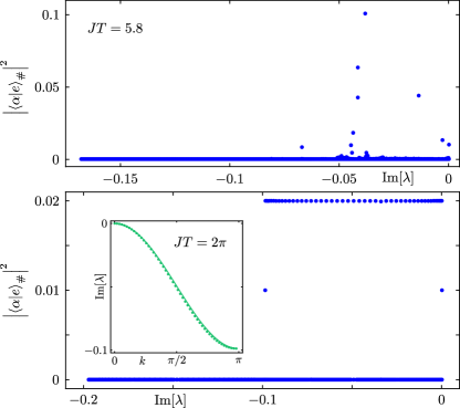
Figure 4: The squared overlap of the eigenoperators of ${\cal F}$ with the edge superket is plotted as a function of the imaginary part of the corresponding eigenvalues. Away from the resonant driving point (top panel), only a few eigenoperators have large values of $|\braket{\alpha}{e}_{\sharp}|^{2}$, leading to an exponential decay. At resonant driving however (bottom panel), many states have a large and equal overlap with the edge, leading to a diffusive decay of the survival probability. We use a ladder of 50 rungs and $\tau/T=1/40$ in both panels. The inset contains only those eigenoperators for which $|\braket{\alpha}{e}_{\sharp}|^{2}>0.005$, using the data from the bottom panel. They are sorted in decreasing order of ${\rm Im}[\lambda]$ as $\lambda_{0}>\lambda_{1}>\ldots>\lambda_{N-1}$ and plotted as a function of $k=\pi j/N$, where $j\in\{0,N-1\}$. For comparison, the solid curve shows the predicted behavior of $\lambda_{\rho}(k)$ from Eq. (57).

Again, from the data shown in the top panel of the figure it is evident that only few eigenoperators have a sizable overlap with the edge superket. Finally, using the numerically obtained eigenoperators and eigenvalues of the Floquet superoperator, we calculate the survival probability of the edge mode using Eq. (43), and find excellent agreement with the analytical result Eq. (52) as shown in Fig. 2.

V.2.4 Diffusive decay for resonant driving

We now turn to exactly resonant driving, where the addition of timing noise leads to diffusive decay of the end state survival probability. Here, we show this explicitly by calculating the eigenoperators and corresponding eigenvalues of the Floquet superoperator that have non-vanishing overlap with the end state and thus contribute to the survival probability in Eq. (43). This calculation is facilitated by the simple form of the jump operators Eq. (46) on resonance. Moreover, since the bulk band of the noiseless Floquet operator is flat, we can work in the basis of lattice sites $\ket{j,s}$ and treat both end and bulk states on the same footing. Thence, we consider for simplicity an infinite chain, where $U_{\rm F}=\mathbbm{1}$ and $\mathcal{U}_{\rm F}=\mathbbm{1}$ is the identity superoperator.

As we show below, the Floquet superoperator is block-diagonal in operator space, and we diagonalize it in the subspace spanned by the projection operators on single lattice sites, $\left\lvert j,s\right\rangle_{\sharp}=\ket{j,s}\bra{j,s}$. Indeed, using the form of the jump operators given in Eq. (46), it is straightforward to check that

$$\begin{split}\mathcal{L}_{1}^{2}\left\lvert j,s\right\rangle_{\sharp}&=2J^{2}\left(\left\lvert j,s\right\rangle_{\sharp}-\left\lvert j-s,-s\right\rangle_{\sharp}\right),\\ \mathcal{L}_{3}^{2}\left\lvert j,s\right\rangle_{\sharp}&=2J^{2}\left(\left\lvert j,s\right\rangle_{\sharp}-\left\lvert j+s,-s\right\rangle_{\sharp}\right),\\ \mathcal{L}_{2}^{2}\left\lvert j,s\right\rangle_{\sharp}&=\mathcal{L}_{4}^{2}\left\lvert j,s\right\rangle_{\sharp}=2J^{2}\left(\left\lvert j,s\right\rangle_{\sharp}-\left\lvert j,-s\right\rangle_{\sharp}\right).\end{split}$$ (53)

The action of the $\mathcal{L}_{i}^{2}$ does not lead out of the spaced spanned by the operators $\left\lvert j,s\right\rangle_{\sharp}$, i.e., $\mathcal{L}_{i}^{2}$ indeed assumes the asserted block-diagonal form. Translational invariance suggests to diagonalize $\mathcal{F}$ in a momentum space basis of superkets $\left\lvert k,s\right\rangle_{\sharp}$ defined by

$$\left\lvert k,s\right\rangle_{\sharp}=\sum_{j}e^{-ikj}\left\lvert j,s\right\rangle_{\sharp},\quad\left\lvert j,s\right\rangle_{\sharp}=\int_{-\pi}^{\pi}\frac{dk}{2\pi}e^{ikj}\left\lvert k,s\right\rangle_{\sharp}.$$ (54)

In this basis, the squared jump superoperators take the form

$$\begin{split}\mathcal{L}_{1}^{2}(k)&=\begin{pmatrix}\braket{k,+}{\mathcal{L}_{1}^{2}}{k,+}_{\sharp}&\braket{k,+}{\mathcal{L}_{1}^{2}}{k,-}_{\sharp}\\ \braket{k,-}{\mathcal{L}_{1}^{2}}{k,+}_{\sharp}&\braket{k,-}{\mathcal{L}_{1}^{2}}{k,-}_{\sharp}\end{pmatrix}\\ &=2J^{2}\begin{pmatrix}1&-e^{ik}\\ -e^{-ik}&1\end{pmatrix},\\ \mathcal{L}_{3}^{2}(k)&=2J^{2}\begin{pmatrix}1&-e^{-ik}\\ -e^{ik}&1\end{pmatrix},\\ \mathcal{L}_{2}^{2}(k)&=\mathcal{L}_{4}^{2}(k)=2J^{2}\left(\mathbbm{1}-\sigma_{x}\right),\end{split}$$ (55)

where $\sigma_{x}$ is the Pauli matrix. It is straightforward to obtain the Floquet superoperator in Eq. (45) (keeping in mind that $\mathcal{U}_{\rm F}=\mathbbm{1}$) and to diagonalize it. Writing the eigenvalues as $e^{-i\lambda(k)}$, we obtain two bands which we denote by $\lambda_{\rho}(k)$ and $\lambda_{\sigma}(k)$, respectively,

$$e^{-i\lambda_{\rho,\sigma}(k)}=\frac{1}{16}e^{-8\kappa^{2}}\left\{10e^{4\kappa^{2}}+3e^{8\kappa^{2}}+3\vphantom{\left[\left(e^{4\kappa^{2}}-1\right)^{2}\right]^{1/2}}\right.\\ -\left(8e^{4\kappa^{2}}-4e^{8\kappa^{2}}-4\right)\cos(k)-\left(2e^{4\kappa^{2}}-e^{8\kappa^{2}}-1\right)\cos(2k)\\ \pm 2\sqrt{2}\left(e^{4\kappa^{2}}-1\right)\cos(k/2)^{2}\left[26e^{4\kappa^{2}}+3e^{8\kappa^{2}}+3\vphantom{\left(e^{4\kappa^{2}}-1\right)^{2}}\right.\\ \left.\left.+4\left(e^{4\kappa^{2}}-1\right)^{2}\cos(k)+\left(e^{4\kappa^{2}}-1\right)^{2}\cos(2k)\right]^{1/2}\right\}.$$ (56)

Both $\lambda_{\rho}(k)$ and $\lambda_{\sigma}(k)$ are purely imaginary, and the imaginary parts encode the decay rates of the respective eigenoperators. For $k\to 0$, $\lambda_{\rho}(k)$ goes to zero quadratically. Thus, the corresponding eigenoperators are long-lived. In contrast, $\mathop{\mathrm{Im}}(\lambda_{\sigma}(k))<0$ for all values of $k$, so that the eigenoperators corresponding to this band decay quickly. These properties can be seen most clearly in the limit of weak timing noise, in which the expressions for $\lambda_{\lambda}(k)$ and $\lambda_{\sigma}(k)$ simplify considerably:

$$\begin{split}\lambda_{\rho}(k)&=-i2\kappa^{2}\left(1-\cos(k)\right)+O(\kappa^{4}),\\ \lambda_{\sigma}(k)&=-i2\kappa^{2}\left(3+\cos(k)\right)+O(\kappa^{4}).\end{split}$$ (57)

The eigenoperators corresponding to the two bands take the form

$$\begin{split}\left\lvert\rho(k)\right\rangle_{\sharp}&=\frac{1}{\sqrt{2}}\left(\left\lvert k,+\right\rangle_{\sharp}+e^{i\phi_{\rho}(k)}\left\lvert k,-\right\rangle_{\sharp}\right),\\ \left\lvert\sigma(k)\right\rangle_{\sharp}&=\frac{1}{\sqrt{2}}\left(\left\lvert k,+\right\rangle_{\sharp}-e^{i\phi_{\sigma}(k)}\left\lvert k,-\right\rangle_{\sharp}\right),\end{split}$$ (58)

i.e., both have equal weight on the states $\left\lvert k,+\right\rangle_{\sharp}$ and $\left\lvert k,-\right\rangle_{\sharp}$, with relative phases between these states that depend on the momentum $k$. At low momenta, $k\to 0$, or weak timing noise, $\kappa\to 0$, both phases vanish, $\phi_{\rho}(k),\phi_{\sigma}(k)\to 0$. Note that we obtain the same structure for the left eigenvectors of $\mathcal{F}$.

These results allow us to calculate the survival probability of localized states analytically. For simplicity, we consider an initial state that is an incoherent superposition of a particle localized on the $+$ and $-$ sublattice sites in the middle of the chain at $j=0$, i.e., $\left\lvert\rho_{0}\right\rangle_{\sharp}=\frac{1}{2}\left(\left\lvert 0,+\right\rangle_{\sharp}+\left\lvert 0,-\right\rangle_{\sharp}\right)$, where the normalization is chosen such that $\mathop{\mathrm{tr}}(\rho_{0})=1$. The overlaps of this density matrix with the left eigenoperators corresponding to the bands $\lambda_{\rho}(k)$ and $\lambda_{\sigma}(k)$ are $\braket{\rho(k)}{\rho_{0}}_{\sharp}=1/\sqrt{2}$ and $\braket{\sigma(k)}{\rho_{0}}_{\sharp}=0$. Moreover, $\left\lvert\rho_{0}\right\rangle_{\sharp}$ has vanishing overlap with any “off-diagonal” operators such as $\ket{j,s}\bra{j^{\prime},s^{\prime}}$. Hence, the survival probability Eq. (43) is given by,

$$P_{\mathrm{s}}=\frac{1}{2}\int_{-\pi}^{\pi}\frac{dk}{2\pi}e^{-in\lambda_{\rho}(k)}.$$ (59)

For $n\to\infty$, the integral over momenta can be evaluated in a stationary-phase approximation. To this end, we expand $\lambda_{\rho}(k)$ in the vicinity of its minimum at $k=0$,

$$\lambda_{\rho}(k)=-\frac{k^{2}}{2}\tanh(2\kappa^{2})+O(k^{4}).$$ (60)

Then, extending the integration over momenta to the full real line, we find

$$s\sim\frac{1}{\sqrt{8\pi n\tanh(2\kappa^{2})}},$$ (61)

i.e., diffusive decay for any value of $\kappa$. At weak noise, we can expand the hyperbolic tangent in $\kappa$ and recover the result of Ref. Rieder et al. (2017). Actually, for $\kappa\to 0$, a closed expression for the survival probability can be obtained over the full range of $n$ by using Eqs. (57). Then, the integral in Eq. (59) yields a modified Bessel function,

$$P_{\mathrm{s}}=\frac{1}{2}\int_{-\pi}^{\pi}\frac{dk}{2\pi}e^{-2n\kappa^{2}\left(1-\cos(k)\right)}=\frac{1}{2}e^{-2n\kappa^{2}}I_{0}(2n\kappa^{2}).$$ (62)

As shown in Fig. 2, this result is in excellent agreement with the numerically determined survival probability. We finally note that using the asymptotic expansion of the Bessel function, $I_{0}(x)\sim e^{x}/\sqrt{2\pi x}$ for $x\to\infty$, leads again to diffusive decay, $P_{\mathrm{s}}\sim 1/(4\kappa\sqrt{\pi n})$ for $n\to\infty$.

Our analytical treatment of the noisy Floquet topological chain at resonant driving shows that the diffusive decay of the end state can be traced back to two key properties of the eigenoperators and eigenvalues of the Floquet superoperator: (i) The end state has spectral weight on a continuum (in the thermodynamic limit) of eigenoperators which form the band $\lambda_{\rho}(k)$, and (ii) the corresponding eigenvalues accumulate at $\lambda=0$. More specifically, the quadratic vanishing of $\lambda_{\rho}(k)$ for $k\to 0$ implies that the “density of states” $\sim 1/(d\lambda_{\rho}(k)/dk)$ has a square-root divergence at $\lambda=0$. These properties, together with the expression for the survival probability Eq. (43), provide an intuitive way of understanding the form of the the end mode decay shown in Fig. 2: The survival probability is obtained by integrating over a continuum of real exponential functions, leading to a diffusive decay.

Figures 3 and 4 show the numerical check of this intuition. In the right panel of Fig. 3, which pertains to resonant driving, we observe that indeed a large number of eigenoperators of ${\cal F}$ have a nonzero overlap with the edge superket. In fact, as illustrated in the bottom panel of Fig. 4, the spectral weight of the edge superket is almost evenly distributed over the set of states forming the band $\lambda_{\rho}(k)$ identified in our analytical approach. This confirms property (i). A first indication of property (ii) can also be seen in the main panel of Fig. 4 – evidently, eigenvalues of $\mathcal{F}$ that have non-zero overlap with $\left\lvert e\right\rangle_{\sharp}$ cluster at $\mathop{\mathrm{Im}}(\lambda)=0$. To demonstrate this feature unambiguously, we plot in the inset of Fig. 4 the imaginary parts of these eigenvalues in decreasing order and find good agreement with the analytical prediction in Eq. (57). This in turn implies that the density of states has a square-root singularity at $k\to 0$, which is rounded in the numerics due to the finite system size.

V.2.5 Diffusive decay for a disorder-localized bulk

As explained above and illustrated in Fig. 2, the decay of the end state survival probability is diffusive if the bulk states are localized. Localization can be due to resonant driving conditions – we considered this fine-tuned situation, which is amenable to a fully analytical treatment, in the previous section. In the more generic case of driving parameters that do not match the resonance condition, localization of the bulk states can be induced by adding disorder to the system, i.e., by modifying the driving protocol Eq. (35) as

$$H(t)=H_{i}+H_{\mathrm{dis}}\quad\text{for}\quad\left(i-1\right)T/4\leq t<iT/4,$$ (63)

where $H_{i}$ and $H_{\mathrm{dis}}$ are given in Eqs. (36) and (38), respectively. The quenched disorder term $H_{\mathrm{dis}}$ does not commute with the clean Hamiltonians $H_{i}$. Therefore, we form superoperators ${\cal H}_{i}$ from the full disordered Hamiltonian during each driving step, $H_{i}+H_{\rm dis}$. This allows us to perform the noise average separately for each quenched disorder realization, and leads again to a Floquet superoperator of the form of Eq. (44), which factorizes into contributions corresponding to the individual driving steps.

While the inclusion of disorder complicates analytics significantly, we can still gain valuable insight from the Floquet superoperator formalism if we determine the spectrum of $\mathcal{F}$ numerically. In particular, above we identified a square-root singularity of the density of states at $\lambda=0$ as the root cause for the diffusive decay. Here, we provide evidence that this phenomenon persists in a disordered system.

Figure. 5 shows the probability distribution of ${\rm Im}[\lambda]$ for all states with an overlap $|\braket{\alpha}{e}_{\sharp}|^{2}>10^{-4}$. When the diffusive decay results from adding disorder to the system, the eigenvalues of ${\cal F}$ take random values for each disorder realization. However, we observe that the distribution is peaked towards $\lambda\to 0$, signifying that there is a large number of slowly decaying states. The peak height grows with increasing system size for the sizes we can access numerically, and its decay away from $\lambda=0$ is comparable to $1/\sqrt{-{\rm Im}[\lambda]}$ (black line). Given the form of the survival probability Eq. (43), a square root singularity leads to a diffusive decay, consistent with Fig. 2.

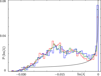
Figure 5: Probability distribution of ${\rm Im}[\lambda]$, ${\cal P}({\rm Im}[\lambda])$, corresponding to all eigenoperators of ${\cal F}$ for which the squared overlap with the edge superket is greater than $10^{-4}$. We use an on-site disorder strength $VT/4=0.4$ and a noise strength $\tau/T=1/80$. The three histograms represent different system sizes: 40 rungs (red), 50 rungs (green), and 60 rungs (blue). They are obtained from 150 simultaneous disorder-noise realizations in the case of 40 and 50 rung systems, and by using 50 realizations for the largest system size. The probability distribution is peaked towards $\lambda\to 0$, with a peak hight that increases with system size. The black curve shows a square root singularity, which by Eq. (43) leads to a diffusive decay of the end mode survival probability.

VI Conclusions and Outlook

In this paper, we discussed a general formalism to treat randomly driven quantum systems with periodically recurring statistics. Our focus was on a description of the averaged system dynamics. We showed that the average over random fluctuations of the drive leads to an evolution equation of the system’s density matrix in terms of a Floquet superoperator (4). The eigenoperators and eigenvalues of the Floquet superoperator are generalizations of Floquet states and quasienergies, which are familiar from the theory of periodically driven systems without noise, to the randomly driven setting. In particular, a spectral representation of the Floquet superoperator in terms of its eigenoperators and their corresponding eigenvalues enables an efficient description of the system dynamics in analogy to the spectral representation of the usual Floquet operator in terms of Floquet states and quasienergies.

We developed this formalism in the context of noisy Floquet systems and showed that it can also be applied in systems with fully random driving. To illustrate the formalism, we revisited a model of a Floquet topological chain which we previously studied in Ref. Rieder et al. (2017), and we re-derived and corroborated our earlier results. Our analysis of the spectrum of the Floquet superoperator revealed that the diffusive decay of the end state of a Floquet topological chain with a localized bulk can be traced back to an accumulation of long-lived modes, i.e., eigenvalues with vanishing imaginary part.

In this work, we focused on piecewise constant driving protocols, for which timing noise is a naturally present source of unwanted random fluctuations. Other types of noise have to be taken into account for continuous driving as is realized, e.g., in laser-induced Floquet topological insulators in condensed matter experiments Wang et al. (2013). In particular, for the simple yet ubiquitous case of harmonic driving described by $H(t)=H_{0}+H_{1}A\sin(\omega t+\phi)$ with time-independent Hamiltonians $H_{0}$ and $H_{1}$, noise might affect the amplitude $A$, frequency $\omega$, and phase $\phi$ of the drive. Which type of noise dominates depends both on the concrete experimental realization and the physical phenomenon under study. From the perspective of theory, an immediate question is whether such a situation can also be described by a Floquet superoperator formalism. We expect that this is the case if the noise is Markovian, i.e., correlations of the noise decay much faster than all other relevant time scales set by the Hamiltonians $H_{0}$ and $H_{1}$, as well as the period of the drive. This expectation is grounded on the observation that our derivation of a formal expression for the Floquet superoperator relied solely on the assumption of statistical independence of fluctuations in different driving cycles, which translates to assuming Markovian correlations for temporally continuous noise processes. The precise form of the Floquet superoperator for amplitude, frequency, and phase noise, and the physical consequences of such types of noise for, e.g., the decay of edge states, are interesting questions for further studies.

Above, we applied the Floquet superoperator formalism to a one-dimensional noisy Floquet topological chain, and it will be interesting to extend this analysis to higher-dimensional Floquet topological phases. As in the one-dimensional case, noise will lead to leakage from topological surface modes into the bulk. However, in contrast to the Floquet topological chain considered here, surface modes in higher-dimensional systems are propagating, and it is an open question how the propagation along the system’s surface will be affected by different types of noise.

Appendix A Implementation of superoperators

To study the properties of the noise-averaged Floquet superoperator $\mathcal{F}$ it is convenient to obtain a matrix representation Zwolak and Vidal (2004). For this purpose we regard density matrices as vectors, “superkets,” in the space of operators. Starting from the lattice-site basis of states $\ket{j,s}$ of the original Hilbert space in the example of Sec. V, a basis of operator space is given by

$$\left\lvert j,s;j^{\prime},s^{\prime}\right\rangle_{\sharp}=\ket{j,s}\bra{j^{\prime},s^{\prime}}.$$ (64)

A scalar product in the space of operators is defined by $\braket{A}{B}_{\sharp}=\mathop{\mathrm{tr}}(A^{\dagger}B)$, which implies

$$\braket{j_{1},s_{1};j_{2},s_{2}}{j_{3},s_{3};j_{4},s_{4}}_{\sharp}\\ \begin{aligned} &=\mathop{\mathrm{tr}}(\ket{j_{2},s_{2}}\braket{j_{1},s_{1}}{j_{3},s_{3}}\bra{j_{4},s_{4}})\\ &=\delta_{j_{1}j_{3}}\delta_{s_{1}s_{3}}\delta_{j_{2}j_{4}}\delta_{s_{2}s_{4}}.\end{aligned}$$ (65)

In the basis of operators $\left\lvert j,s;j^{\prime},s^{\prime}\right\rangle_{\sharp}$, the matrix elements of the superoperator $\mathcal{H}_{i}$, which is defined by its action on an operator $A$, $\mathcal{H}_{i}A=[H_{i},A]$, are thus given by

$$\braket{j_{1},s_{1};j_{2},s_{2}}{\mathcal{H}_{i}}{j_{3},s_{3};j_{4},s_{4}}_{\sharp}\\ \begin{aligned} &=\mathop{\mathrm{tr}}(\ket{j_{2},s_{2}}\bra{j_{1},s_{1}}[H_{i},\ket{j_{3},s_{3}}\bra{j_{4},s_{4}}])\\ &=\bra{j_{1},s_{1}}[H_{i},\ket{j_{3},s_{3}}\bra{j_{4},s_{4}}]\ket{j_{2},s_{2}}\\ &=\braket{j_{1},s_{1}}{H_{i}}{j_{3},s_{3}}\delta_{j_{4}j_{2}}\delta_{s_{4}s_{2}}\\ &\mathrel{\hphantom{=}}-\delta_{j_{1}j_{3}}\delta_{s_{1}s_{3}}\braket{j_{4},s_{4}}{H_{i}}{j_{2},s_{2}}.\end{aligned}$$ (66)

With the matrix representation of the superoperators $\mathcal{H}_{i}$ for $i=1,2,3,4$, it is straightforward to assemble the Floquet superoperator $\mathcal{F}$ [Eq. (44)] for the noisy Floquet topological chain discussed in Sec. V. All numerical results presented in that section are based on the exact diagonalization of the Floquet superoperator.

References

- Eckardt (2017) A. Eckardt, “Colloquium: Atomic quantum gases in periodically driven optical lattices,” Reviews of Modern Physics 89, 011004 (2017), arXiv:1606.08041 .
- Rahav et al. (2003a) S. Rahav, I. Gilary, and S. Fishman, “Effective Hamiltonians for periodically driven systems,” Phys. Rev. A - At. Mol. Opt. Phys. 68, 18 (2003a), arXiv:0301033 [nlin] .
- Rahav et al. (2003b) S. Rahav, I. Gilary, and S. Fishman, “Time independent description of rapidly oscillating potentials,” Phys. Rev. Lett. 91, 1–4 (2003b), arXiv:0302023 [nlin] .
- Goldman and Dalibard (2014) N. Goldman and J. Dalibard, “Periodically driven quantum systems: Effective Hamiltonians and engineered gauge fields,” Phys. Rev. X 4, 1–29 (2014), arXiv:1404.4373 .
- Kitagawa et al. (2010) T. Kitagawa, E. Berg, M. Rudner, and E. Demler, “Topological characterization of periodically driven quantum systems,” Phys. Rev. B 82, 235114 (2010).
- Rudner et al. (2013) M. S. Rudner, N. H. Lindner, E. Berg, and M. Levin, “Anomalous edge states and the bulk-edge correspondence for periodically driven two-dimensional systems,” Phys. Rev. X 3, 031005 (2013).
- Rieder et al. (2017) M. T. Rieder, L. M. Sieberer, M. H. Fischer, and I. C. Fulga, “Localization counteracts decoherence in noisy Floquet topological chains,” Phys. Rev. Lett. 120, 216801 (2017), arXiv:1711.06188 .
- Haake (2010) F. Haake, Quantum Signatures of Chaos, Springer Series in Synergetics, Vol. 54 (Springer Berlin Heidelberg, Berlin, Heidelberg, 2010).
- Mukherjee et al. (2017) S. Mukherjee, A. Spracklen, M. Valiente, E. Andersson, P. Öhberg, N. Goldman, and R. R. Thomson, “Experimental observation of anomalous topological edge modes in a slowly driven photonic lattice,” Nature Communications 8, 13918 EP – (2017).
- Maczewsky et al. (2017) L. J. Maczewsky, J. M. Zeuner, S. Nolte, and A. Szameit, “Observation of photonic anomalous floquet topological insulators,” Nature Communications 8, 13756 EP – (2017).
- Longhi (2009) S. Longhi, “Quantum-optical analogies using photonic structures,” Laser & Photonics Reviews 3, 243–261 (2009).
- Szameit and Nolte (2010) A. Szameit and S. Nolte, “Discrete optics in femtosecond-laser-written photonic structures,” J. Phys. B 43, 163001 (2010).
- Oskay et al. (2003) W. H. Oskay, D. A. Steck, and M. G. Raizen, “Timing noise effects on dynamical localization,” in Chaos, Solitons and Fractals, Vol. 16 (2003) pp. 409–416.
- Bitter and Milner (2016) M. Bitter and V. Milner, “Experimental Observation of Dynamical Localization in Laser-Kicked Molecular Rotors,” Phys. Rev. Lett. 117, 144104 (2016), arXiv:1603.06918 .
- Bitter and Milner (2017) M. Bitter and V. Milner, “Control of quantum localization and classical diffusion in laser-kicked molecular rotors,” Phys. Rev. A 95, 013401 (2017).
- ČadeŽ et al. (2017) T. ČadeŽ, R. Mondaini, and P. D. Sacramento, “Dynamical localization and the effects of aperiodicity in Floquet systems,” Phys. Rev. B 96, 1–9 (2017), arXiv:1707.07420 .
- Cadez et al. (2018) T. Cadez, R. Mondaini, and P. D. Sacramento, “Edge and bulk localization of Floquet topological superconductors,” (2018), arXiv:1808.10238 .
- Reimer et al. (2018) V. Reimer, K. G. L. Pedersen, N. Tanger, M. Pletyukhov, and V. Gritsev, “Nonadiabatic effects in periodically driven dissipative open quantum systems,” Phys. Rev. A 97, 043851 (2018).
- Schnell et al. (2018) A. Schnell, A. Eckardt, and S. Denisov, “Is there a Floquet Lindbladian?” (2018), arXiv:1809.11121 .
- Zoller et al. (1981) P. Zoller, G. Alber, and R. Salvador, “ac Stark splitting in intense stochastic driving fields with Gaussian statistics and non-Lorentzian line shape,” Phys. Rev. A 24, 398–410 (1981).
- Hu et al. (2015) Y. Hu, Z. Cai, M. A. Baranov, and P. Zoller, “Majorana fermions in noisy Kitaev wires,” Phys. Rev. B - Condens. Matter Mater. Phys. 92, 1–13 (2015), arXiv:1506.06977 .
- Cai et al. (2016) Z. Cai, C. Hubig, and U. Schollwöck, “Universal long-time behavior of stochastically driven interacting quantum systems,” 1609.08518 96, 1–13 (2016), arXiv:1609.08518 .
- Zwolak and Vidal (2004) M. Zwolak and G. Vidal, “Mixed-state dynamics in one-dimensional quantum lattice systems: A time-dependent superoperator renormalization algorithm,” Phys. Rev. Lett. 93, 1–4 (2004), arXiv:0406440 [cond-mat] .
- Wang et al. (2013) Y. H. Wang, H. Steinberg, P. Jarillo-Herrero, and N. Gedik, “Observation of floquet-bloch states on the surface of a topological insulator,” Science (80-. ). 342, 453–457 (2013), arXiv:1310.7563 .