Phenomenology of A Little Higgs Pseudo-Axion

Abstract

In models where the Higgs is realized as a pseudo-Nambu-Goldstone boson (pNGB) of some global symmetry breaking, there are often remaining pNGBs of some $U(1)$ groups (called “pseudo-axions”), which could lead to smoking gun signatures of such scenarios and provide important clues on the electroweak symmetry breaking mechanism. As a concrete example, we investigate the phenomenology of the pseudo-axion in the anomaly-free Simplest Little Higgs (SLH) model. After clarifying a subtle issue related to the effect of symmetric vector-scalar-scalar (VSS) vertices (e.g. $Z_{\mu}(H\partial^{\mu}\eta+\eta\partial^{\mu}H)$), we show that for natural region in the parameter space, the SLH pseudo-axion is top-philic, decaying almost exclusively to a pair of top quarks. The direct and indirect (i.e. via heavy particle decay) production of such a pseudo-axion at the $14~{}{\mbox{TeV}}$ (HL-)LHC turn out to suffer from either large backgrounds or small rates, making its detection quite challenging. A $pp$ collider with higher energy and luminosity, such as the $27~{}{\mbox{TeV}}$ HE-LHC, or even the $100~{}{\mbox{TeV}}$ FCC-hh or SppC, is therefore motivated to capture the trace of such a pNGB.

I Introduction

Despite the great success of the Standard Model (SM), marked by the discovery of the $125~{}{\mbox{GeV}}$ Higgs-like boson Aad:2012tfa ; Chatrchyan:2012xdj and the on-going measurements of its properties, how the SM is embedded into a larger theory still remains a mystery. Since the Higgs boson mass parameter is in general not protected under radiative correction, a naive embedding would signal a high sensitivity of infrared (IR) parameters (the electroweak scale and the Higgs boson mass) to ultraviolet (UV) parameters (i.e. physical parameters defined at a high scale). Although this fine-tuned situation is logically possible, or might be explained to some extent by anthropic reasoning Schellekens:2013bpa ; Donoghue:2016tjk , it is nevertheless natural to conjecture the existence of some systematic mechanism which protects the Higgs boson mass parameter from severe radiative instability. A well-known example of such systematic mechanism is supersymmetry, which has the merit of being weakly-coupled and thus offers better calculability compared to scenarios based on strong dynamics. However supersymmetry requires the introduction of a large number of new degrees of freedom, and a large number of new parameters associated with them, making the model quite cumbersome. None of the new degrees of freedom have been observed. It is therefore well-motivated to consider alternative but simpler mechanisms with weakly-coupled dynamics in their range of validity.

One candidate of such alternative is the Little Higgs mechanism ArkaniHamed:2001nc ; ArkaniHamed:2002pa ; ArkaniHamed:2002qx ; ArkaniHamed:2002qy , in which the Higgs boson is a Goldstone boson of some spontaneous global symmetry breaking. The global symmetry is also explicitly broken in a collective manner such that the Higgs boson acquires a mass and at the same time the model is radiatively more stable. A very simple implementation of this collective symmetry breaking (CSB) idea is the Simplest Little Higgs (SLH) model Kaplan:2003uc ; Schmaltz:2004de , in which the electroweak gauge group is enlarged to $SU(3)_{L}\times U(1)_{X}$, and two scalar triplets are introduced to realize the global symmetry breaking pattern

$$[SU(3)_{1}\times U(1)_{1}]\times[SU(3)_{2}\times U(1)_{2}]$$

$$\rightarrow[SU(2)_{1}\times U(1)_{1}]\times[SU(2)_{2}\times U(1)_{2}]$$ (1)

The global symmetry is also explicitly broken by gauge and Yukawa interactions, but in a collective manner to improve the radiative stability of the scalar sector. The particle content is quite economical. Especially in the low energy scalar sector, there exists only two physical degrees of freedom, one of which (denoted $H$) could be identified with the $125~{}{\mbox{GeV}}$ Higgs-like particle, while the other is a CP-odd scalar $\eta$ which is referred to as a pseudo-axion in the literature Kilian:2004pp ; Kilian:2006eh .

In the SLH, the pseudo-axion $\eta$ is closely related to the electroweak symmetry breaking (EWSB) and therefore studying its phenomenology is well-motivated. According to the hidden mass relation derived in ref. Cheung:2018iur , the $\eta$ mass $m_{\eta}$ is anti-correlated with the top partner mass $m_{T}$, which is in turn related to the degree of fine-tuning in the model. The hidden mass relation is derived within an approach consistent with the continuum effective field theory (CEFT) and does not rely on the assumption on the contribution from the physics at the cutoff. Although phenomenology of the $\eta$ particle has been studied by quite a few papers (e.g. Kilian:2004pp ; Kilian:2006eh ; Cheung:2006nk ; Cheung:2008zu ; Han:2013ic ), their treatment was not based on the hidden mass relation, and also most of the papers were written before the $125~{}{\mbox{GeV}}$ boson was discovered. It is thus timely to revisit the status of $\eta$ phenomenology in light of the discovery of the $125~{}{\mbox{GeV}}$ boson, taking into account the properly derived hidden mass relation and focusing on the parameter space favored by naturalness considerations.

There is another important reason that warrants a reanalysis of the $\eta$ phenomenology. The SLH is usually written as a gauged nonlinear sigma model, in which the EWSB can be parametrized through vacuum misalignment. However, the vacuum misalignment also leads to the fact that, in the usual parametrization of the two scalar triplets, there exist scalar kinetic terms that are not canonically-normalized, and vector-scalar two-point transitions that are “unexpected” He:2017jjx . A further field rotation, including an appropriate gauge-fixing procedure, is thus required to properly diagonalize the vector-scalar sector of the SLH model. This subtlety had been overlooked in all related papers before ref. He:2017jjx , and if one carries out a proper diagonalization of the bosonic sector of the SLH, some of the $\eta$-related couplings will turn out to be different from what has been obtained in previous literature. This is the case for both the $ZH\eta$ coupling and the coupling of $\eta$ to a pair of SM fermions. The occurrence of the mass eigenstate antisymmetric $ZH\eta$ vertex (i.e. $Z_{\mu}(H\partial^{\mu}\eta-\eta\partial^{\mu}H)$) is postponed to $\mathcal{O}(\xi^{3})$ (with $\xi\equiv\frac{v}{f}$, $v\approx 246~{}{\mbox{GeV}}$ and $f$ is the global symmetry breaking scale of Eq. (1)), and the couplings of $\eta$ to a pair of SM charged leptons, and to $b\overline{b},c\overline{c},u\overline{u}$ are found to vanish to all order in $\xi$. This leads to significant changes in the $\eta$ phenomenology, which will be studied in detail in this work.

When one tries to derive the $\eta$-related Lagrangian in the SLH, symmetric vector-scalar-scalar (VSS) vertices, e.g. $Z_{\mu}(H\partial^{\mu}\eta+\eta\partial^{\mu}H)$ naturally appear, which is a feature that is often present in models based on a nonlinearly-realized scalar sector. The effects of such symmetric VSS vertices contain some subtleties which, to our knowledge, have not been discussed before in literature. Therefore, we devote one section to the analysis of symmetric VSS vertices, which could also be helpful to clarify similar situations in other nonlinearly-realized models.

In this work we do not aim to give a complete characterization of the $\eta$ phenomenology, which could be very complicated in certain corner of parameter space. Instead, we focus our attention on the parameter space favored by naturalness considerations. More specifically, we will consider $\eta$ mass in the region $2m_{t}\lesssim m_{\eta}\lesssim 1~{}{\mbox{TeV}}$, which is favored by naturalness. We then calculate the $\eta$ decay and production at future high energy hadron colliders in various channels. It turns out at the $14~{}{\mbox{TeV}}$ (HL)-LHC the detection of $\eta$ is quite challenging due to various suppression mechanisms. A $pp$ collider with higher energy and luminosity, such as the $27~{}{\mbox{TeV}}$ HE-LHC, or even the $100~{}{\mbox{TeV}}$ FCC-hh or SppC, is therefore motivated to capture the trace of such a pNGB.

The paper is organized as follows. In Section II we review the basic ingredients of the SLH, including the crucial hidden mass relation obtained from a CEFT analysis, and present the mass eigenstate Lagrangian relevant for phenomenological studies. In Section III we clarify the effect of symmetric VSS vertices. Then in Section IV we derive important constraints from electroweak precision observables relevant for the pseudo-axion phenomenology. Section V is dedicated to the study of $\eta$ decay and production at hadron colliders. In Section VI we present the discussion and conclusions.

II The Simplest Little Higgs

II.1 Overview of the Simplest Little Higgs

In the SLH, the electroweak gauge group is enlarged to $SU(3)_{L}\times U(1)_{X}$. Two scalar triplets $\Phi_{1},\Phi_{2}$ are introduced to realize the spontaneous global symmetry breaking pattern in Eq. (1). They are parameterized as

$$\Phi_{1}=\exp\left(\frac{i\Theta^{\prime}}{f}\right)\exp\left(\frac{it_{\beta}\Theta}{f}\right)\begin{pmatrix}0\\ 0\\ fc_{\beta}\end{pmatrix}$$ (2)

$$\Phi_{2}=\exp\left(\frac{i\Theta^{\prime}}{f}\right)\exp\left(-\frac{i\Theta}{ft_{\beta}}\right)\begin{pmatrix}0\\ 0\\ fs_{\beta}\end{pmatrix}$$ (3)

Here we have introduced the shorthand notation $s_{\beta}\equiv\sin\beta,c_{\beta}\equiv\cos\beta,t_{\beta}\equiv\tan\beta$. $f$ is the Goldstone decay constant. $\Theta$ and $\Theta^{\prime}$ are $3\times 3$ matrix fields, parameterized as

$$\Theta=\frac{\eta}{\sqrt{2}}+\begin{pmatrix}\textbf{0}_{2\times 2}&h\\ h^{\dagger}&0\end{pmatrix},\quad\Theta^{\prime}=\frac{\zeta}{\sqrt{2}}+\begin{pmatrix}\textbf{0}_{2\times 2}&k\\ k^{\dagger}&0\end{pmatrix}$$ (4)

$\eta$ is the pseudo-axion, and $h$ and $k$ are parameterized as ($v$ denotes the vacuum expectation value (vev) of the Higgs doublet)

$$h =\begin{pmatrix}h^{0}\\ h^{-}\end{pmatrix},\quad h^{0}=\frac{1}{\sqrt{2}}(v+H-i\chi)$$ (5)

$$k =\begin{pmatrix}k^{0}\\ k^{-}\end{pmatrix},\quad k^{0}=\frac{1}{\sqrt{2}}(\sigma-i\omega)$$ (6)

For future convenience, we introduce the notation

$$\hat{h}\equiv(h^{\dagger}h)^{1/2}$$ (7)

We note that the spontaneous global symmetry breaking Eq. (1) should deliver 10 Goldstone bosons, which are parameterized here in $\Theta$ and $\Theta^{\prime}$. The electroweak gauge group $SU(3)_{L}\times U(1)_{X}$ will eventually break to $U(1)_{EM}$, and therefore 8 Goldstone bosons will be eaten to make the associated gauge bosons massive. Only two Goldstone bosons remain physical, parameterized here as $h$ and $\eta$. The parametrization of these Goldstone fields actually has some freedom, which we refer the reader to ref. Cheung:2018iur for explanation.

In the SLH, under the full gauge group $SU(3)_{C}\times SU(3)_{L}\times U(1)_{X}$, $\Phi_{1}$ and $\Phi_{2}$ have quantum number $(\textbf{1},\textbf{3})_{-\frac{1}{3}}$. The gauge kinetic term of $\Phi_{1}$ and $\Phi_{2}$ can thus be written as

$$\mathcal{L}_{gk}=(D_{\mu}\Phi_{1})^{\dagger}(D^{\mu}\Phi_{1})+(D_{\mu}\Phi_{2})^{\dagger}(D^{\mu}\Phi_{2})$$ (8)

in which the covariant derivative can be expressed as

$$D_{\mu}=\partial_{\mu}-igA_{\mu}^{a}T^{a}+ig_{x}Q_{x}B_{\mu}^{x},\quad g_{x}=\frac{gt_{W}}{\sqrt{1-t_{W}^{2}/3}}$$ (9)

In the above equation, $A_{\mu}^{a}$ and $B_{\mu}^{x}$ denote $SU(3)_{L}$ and $U(1)_{X}$ gauge fields, respectively. $g$ and $g_{x}$ denote the coupling constants of $SU(3)_{L}$ and $U(1)_{X}$ gauge groups, respectively. It is convenient to trade $g_{x}$ for $t_{W}\equiv\tan\theta_{W}$. $T^{a}=\frac{\lambda^{a}}{2}$ where $\lambda^{a},a=1,...,8$ denote the Gell-Mann matrices. For $\Phi_{1},\Phi_{2}$, $Q_{x}=-\frac{1}{3}$. Following ref. delAguila:2011wk , we parameterize the $SU(3)_{L}$ gauge bosons as

$$A_{\mu}^{a}T^{a} =\frac{A_{\mu}^{3}}{2}\begin{pmatrix}1&0&0\\ 0&-1&0\\ 0&0&0\end{pmatrix}$$

$$+\frac{A_{\mu}^{8}}{2\sqrt{3}}\begin{pmatrix}1&0&0\\ 0&1&0\\ 0&0&-2\end{pmatrix}+\frac{1}{\sqrt{2}}\begin{pmatrix}0&W_{\mu}^{+}&Y_{\mu}^{0}\\ W_{\mu}^{-}&0&X_{\mu}^{-}\\ Y_{\mu}^{0\dagger}&X_{\mu}^{+}&0\end{pmatrix}$$ (10)

with the first-order neutral gauge boson mixing relation ($c_{W}\equiv\cos\theta_{W},s_{W}\equiv\sin\theta_{W}$)

$$\begin{pmatrix}A^{3}\\ A^{8}\\ B^{x}\end{pmatrix}=\begin{pmatrix}0&c_{W}&-s_{W}\\ \sqrt{1-\frac{t_{W}^{2}}{3}}&\frac{s_{W}t_{W}}{\sqrt{3}}&\frac{s_{W}}{\sqrt{3}}\\ -\frac{t_{W}}{\sqrt{3}}&s_{W}\sqrt{1-\frac{t_{W}^{2}}{3}}&c_{W}\sqrt{1-\frac{t_{W}^{2}}{3}}\end{pmatrix}\begin{pmatrix}Z^{\prime}\\ Z\\ A\end{pmatrix}$$ (11)

Since the electroweak gauge group is enlarged to $SU(3)_{L}\times U(1)_{X}$, it is also necessary to enlarge the fermion sector in order that fermions transform properly under the enlarged group. We adopt the elegant anomaly-free embedding proposed in ref. Kong:2003vm ; Schmaltz:2004de ; Kong:2004cv . In the lepton Yukawa sector, the SM left-handed lepton doublets are enlarged to $SU(3)_{L}$ triplets $L_{m}=(\nu_{L},\ell_{L},iN_{L})_{m}^{T}$ with $Q_{x}=-\frac{1}{3}$ ($m=1,2,3$ is the family index). There are also right-handed singlet lepton fields $\ell_{Rm}$ with $Q_{x}=-1$ and $N_{Rm}$ with $Q_{x}=0$. The lepton Yukawa Lagrangian can be written as delAguila:2011wk

$$\mathcal{L}_{LY}=i\lambda_{N}^{m}\bar{N}_{Rm}\Phi_{2}^{\dagger}L_{m}+\frac{i\lambda_{\ell}^{mn}}{\Lambda}\bar{\ell}_{Rm}\epsilon_{ijk}\Phi_{1}^{i}\Phi_{2}^{j}L_{n}^{k}+\text{h.c.}$$ (12)

In the quark sector, we have the following field content

$$Q_{1} =(d_{L},-u_{L},iD_{L})^{T},\quad d_{R},\quad u_{R},\quad D_{R}$$ (13)

$$Q_{2} =(s_{L},-c_{L},iS_{L})^{T},\quad s_{R},\quad c_{R},\quad S_{R}$$ (14)

$$Q_{3} =(t_{L},b_{L},iT_{L})^{T},\quad t_{R},\quad b_{R},\quad T_{R}$$ (15)

Here $Q_{1},Q_{2}$ transform under $\bar{\textbf{3}}$ representation of $SU(3)_{L}$ with $Q_{x}=0$. $Q_{3}$ transforms under 3 representation of $SU(3)_{L}$ with $Q_{x}=\frac{1}{3}$. The right-handed quark fields are all $SU(3)_{L}$ singlets with various $U(1)_{X}$ charges. More specifically, $u_{R},c_{R},t_{R},T_{R}$ carry $Q_{x}=\frac{2}{3}$ while $d_{R},s_{R},b_{R},D_{R},S_{R}$ carry $Q_{x}=-\frac{1}{3}$. The quark Yukawa Lagrangian can be written as delAguila:2011wk

$$\mathcal{L}_{QY} =i\lambda_{1}^{t}\bar{u}_{R3}^{1}\Phi_{1}^{\dagger}Q_{3}+i\lambda_{2}^{t}\bar{u}_{R3}^{2}\Phi_{2}^{\dagger}Q_{3}$$

$$+i\frac{\lambda_{b}^{m}}{\Lambda}\bar{d}_{Rm}\epsilon_{ijk}\Phi_{1}^{i}\Phi_{2}^{j}Q_{3}^{k}+i\lambda_{1}^{dn}\bar{d}_{Rn}^{1}Q_{n}^{T}\Phi_{1}$$

$$+i\lambda_{2}^{dn}\bar{d}_{Rn}^{2}Q_{n}^{T}\Phi_{2}+i\frac{\lambda_{u}^{mn}}{\Lambda}\bar{u}_{Rm}\epsilon_{ijk}\Phi_{1}^{*i}\Phi_{2}^{*j}Q_{n}^{k}+\text{h.c.}$$ (16)

In the above equation, $n=1,2$ is the family index for the first two generations of quark triplets. $d_{Rm}$ runs over $(d_{R},s_{R},b_{R},D_{R},S_{R})$ and $u_{Rm}$ runs over $(u_{R},c_{R},t_{R},T_{R})$. $u_{R3}^{1},u_{R3}^{2}$ are linear combinations of $t_{R}$ and $T_{R}$. $d_{Rn}^{1},d_{Rn}^{2}$ are linear combinations of $d_{R}$ and $D_{R}$ for $n=1$ and of $s_{R}$ and $S_{R}$ for $n=2$. It is worth noting that in the dimension-4 part of the Eq. (12) and Eq. (16) CSB is formally preserved. In contrast, in Eq. (12) and Eq. (16), the dimension-5 part formally violates CSB. Nevertheless the amount of violation is proportional to light fermion Yukawas and is thus negligible.

We now turn to the scalar potential. Using a CEFT approach and combining tree level and one-loop contributions, the scalar effective potential in the SLH is calculated to be Cheung:2018iur

$$V=-\mu^{2}(\Phi_{1}^{\dagger}\Phi_{2}+\Phi_{2}^{\dagger}\Phi_{1})+\lambda|\Phi_{1}^{\dagger}\Phi_{2}|^{2}+\Delta(\hat{h})\hat{h}^{4}$$ (17)

$\mu^{2}$ and $\lambda$ could be regarded as parameters to be determined from experiments, while $\Delta(\hat{h})$ is automatically finite, and could be expressed from Lagrangian parameters in the model

$$\Delta(\hat{h}) =\frac{3}{16\pi^{2}}\Bigg{\{}\lambda_{t}^{4}\left[\ln\frac{M_{T}^{2}}{m_{t}^{2}(\hat{h})}-\frac{1}{2}\right]$$

$$-\frac{1}{8}g^{4}\left[\ln\frac{M_{X}^{2}}{m_{W}^{2}(\hat{h})}-\frac{1}{2}\right]$$

$$-\frac{1}{16}g^{4}(1+t_{W}^{2})^{2}\left[\ln\frac{M_{Z^{\prime}}^{2}}{m_{Z}^{2}(\hat{h})}-\frac{1}{2}\right]\Bigg{\}}$$ (18)

$\lambda_{t}$ is defined as

$$\lambda_{t}\equiv\frac{\lambda_{1}^{t}\lambda_{2}^{t}}{\sqrt{\lambda_{1}^{t2}c_{\beta}^{2}+\lambda_{2}^{t2}s_{\beta}^{2}}}$$ (19)

where $\lambda_{1}^{t},\lambda_{2}^{t}$ are the two Yukawa couplings in the top sector, introduced in Eq. (16). $M_{T}^{2},M_{X}^{2},M_{Z^{\prime}}^{2}$ are defined as

$$M_{T}^{2} \equiv(\lambda_{1}^{t2}c_{\beta}^{2}+\lambda_{2}^{t2}s_{\beta}^{2})f^{2}$$ (20)

$$M_{X}^{2} \equiv\frac{1}{2}g^{2}f^{2}$$ (21)

$$M_{Z^{\prime}}^{2} \equiv\frac{2}{3-t_{W}^{2}}g^{2}f^{2}$$ (22)

They are related to physical mass squared of the relevant particles as follows

$$M_{T}^{2} =m_{T}^{2}+m_{t}^{2}$$ (23)

$$M_{X}^{2} =m_{X}^{2}+m_{W}^{2}$$ (24)

$$M_{Z^{\prime}}^{2} =m_{Z^{\prime}}^{2}+m_{Z}^{2}$$ (25)

in which $m_{T},m_{t}$ denote the physical mass of the heavy top $T$ and the top quark $t$, $m_{X},m_{W}$ denote the physical mass of the $X$ boson and $W$ boson, $m_{Z^{\prime}},m_{Z}$ denote the physical mass of the $Z^{\prime}$ boson and $Z$ boson, respectively. $m_{t}^{2}(\hat{h}),m_{W}^{2}(\hat{h}),m_{Z}^{2}(\hat{h})$ are field-dependent mass squared, which we use the following leading order (LO) expression

$$m_{t}^{2}(\hat{h}) =\lambda_{t}^{2}\hat{h}^{2}$$ (26)

$$m_{W}^{2}(\hat{h}) =\frac{1}{2}g^{2}\hat{h}^{2}$$ (27)

$$m_{Z}^{2}(\hat{h}) =\frac{1}{2}g^{2}(1+t_{W}^{2})\hat{h}^{2}$$ (28)

With the above expressions for the scalar effective potential we are able to compute the electroweak vev, Higgs mass, pseudo-axion mass, etc. as a function of $\mu^{2},\lambda$ and other Lagrangian parameters in the model.

Finally we note that there of course exist gauge-invariant kinetic Lagrangian for the $SU(3)_{L}\times U(1)_{X}$ gauge fields and the fermion fields in the model, according to their representations.

II.2 Hidden Mass Relation, Unitarity and Naturalness

Before starting the phenomenological analysis in the SLH, it is important to notice that there exist certain constraints that we have to take into account Cheung:2018iur .

First, there exists a hidden mass relation which follows from an analysis of the scalar effective potential Eq. (17). This is because if we consider $g,t_{W},\lambda_{t}$ as fixed, then the scalar effective potential Eq. (17) is fully determined by 5 parameters, say $\mu^{2},\lambda,f,t_{\beta},m_{T}$. Requiring electroweak vev to be $246~{}{\mbox{GeV}}$ and the CP-even Higgs mass to be $125~{}{\mbox{GeV}}$ should eliminate two parameters, leaving only three parameters as independent. For instance, we may choose $f,t_{\beta},m_{T}$ as the three independent parameters, then any other observable could be expressed in terms of these three parameters. Especially, the pseudo-axion mass $m_{\eta}$ is determined from the following hidden mass relation derived in ref. Cheung:2018iur

$$m_{\eta}^{2}=[m_{h}^{2}-v^{2}\Delta_{A}(3-2\theta t_{2\theta}^{-1})+v^{2}A(5-2\theta t_{2\theta}^{-1})]s_{\theta}^{-2}$$ (29)

Here $t_{2\theta}^{-1}\equiv\frac{1}{\tan(2\theta)},s_{\theta}^{-2}\equiv\frac{1}{\sin^{2}\theta}$, and $\theta,A,\Delta_{A}$ are defined by

$$\theta\equiv\frac{v}{\sqrt{2}fs_{\beta}c_{\beta}}$$ (30)

$$A\equiv\frac{3}{16\pi^{2}}\left[\lambda_{t}^{4}-\frac{g^{4}}{8}-\frac{g^{4}}{16}(1+t_{W}^{2})^{2}\right]$$ (31)

$$\Delta_{A} \equiv\frac{3}{16\pi^{2}}\Bigg{[}\lambda_{t}^{4}\ln\frac{M_{T}^{2}}{m_{t}^{2}}-\frac{g^{4}}{8}\ln\frac{M_{X}^{2}}{m_{W}^{2}}$$

$$-\frac{g^{4}}{16}(1+t_{W}^{2})^{2}\ln\frac{M_{Z^{\prime}}^{2}}{m_{Z}^{2}}\Bigg{]}$$ (32)

The basic feature of this mass relation is that the pseudo-axion mass is anti-correlated with the top partner mass.

Second, the SLH is meant to be only an effective field theory valid up to some energy scale, which could be revealed by an analysis of partial wave unitarity. This is done in ref. Cheung:2018iur and the unitarity cutoff is determined to be

$$\Lambda_{U}=\sqrt{8\pi}\times\min\{fc_{\beta},fs_{\beta}\}$$ (33)

Apart from the lepton Yukawa part, the SLH Lagrangian is manifestly symmetric with respect to the exchange $\Phi_{1}\leftrightarrow\Phi_{2}$ (with the corresponding exchange of all related coefficients), therefore without loss of generality we may restrict to $t_{\beta}\geq 1$. The resulting formulae have the $t_{\beta}\leftrightarrow\frac{1}{t_{\beta}}$ invariance. Nevertheless, the lepton Yukawa Lagrangian Eq. (12) does not share this exchange symmetry, and the $t_{\beta}\leftrightarrow\frac{1}{t_{\beta}}$ invariance could be lost. However, if we do not deal directly with lepton-related vertices, the $t_{\beta}\leftrightarrow\frac{1}{t_{\beta}}$ invariance violation could only come from input parameter corrections, which are all suppressed by $\frac{v^{2}}{f^{2}}$ Cheung:2018iur , which is a very small quantity if we consider current bound on $f$. Therefore in the following, unless otherwise specified, we will assume $t_{\beta}\geq 1$. (Moreover, in Section IV we will show that the $t_{\beta}<1$ case is disfavored by electroweak precision measurements for natural region of parameter space.) Then we can express the unitarity cutoff as

$$\Lambda_{U}=\sqrt{8\pi}fc_{\beta}$$ (34)

and we require all particle masses be less than $\Lambda_{U}$. We note that since $\Lambda_{U}$ is determined by the smaller of the triplet vevs, while $m_{Z^{\prime}}$ is determined by the quadrature of the triplet vevs, therefore requiring $m_{Z^{\prime}}\leq\Lambda_{U}$ leads to an upper bound on $t_{\beta}$ (besides our assumption $t_{\beta}\geq 1$)

$$1\leq t_{\beta}\leq\sqrt{\frac{4\pi(3-t_{W}^{2})}{g^{2}}-1}\approx 8.9$$ (35)

Third, the parameter $M_{T}$ has a lower bound derived simply from the structure of the Yukawa Lagrangian Han:2005ru

$$M_{T}\geq\sqrt{2}\frac{m_{t}}{v}fs_{2\beta}\approx fs_{2\beta}$$ (36)

where $s_{2\beta}\equiv\sin(2\beta)$. $M_{T}$ is also bounded from above by either $\Lambda_{U}$ or the requirement that $m_{\eta}^{2}$ obtained from Eq. (29) should be positive.

Finally, from the LHC search of $Z^{\prime}$ boson in the dilepton channel Aaboud:2017buh ; Sirunyan:2018exx , we estimate the lower bound on $f$ as Mao:2017hpp

$$f\gtrsim 7.5~{}{\mbox{TeV}}$$ (37)

We note that when combined with Eq. (36) and Eq. (35) this also leads to a lower bound on the top partner mass of around $1.7~{}{\mbox{TeV}}$, which is much more stringent than constraints from top partner searches at the LHC.

It is remarkable that the naturalness issue can also be analyzed in a CEFT approach, which is done in ref. Cheung:2018iur . We define the total degree of fine-tuning at a certain parameter point as

$$\Delta_{\text{TOT}}=\max\{\Delta_{\text{TOT}}^{\mu^{2}},\Delta_{\text{TOT}}^{\lambda}\}$$ (38)

where $\Delta_{\text{TOT}}^{\mu^{2}},\Delta_{\text{TOT}}^{\lambda}$ are defined by

$$\Delta_{\text{TOT}}^{\lambda}\equiv\left|\frac{\lambda_{U}}{m_{h}^{2}}\frac{\partial m_{h}^{2}}{\partial\lambda_{U}}\right|,\quad\Delta_{\text{TOT}}^{\mu^{2}}\equiv\left|\frac{\mu_{U}^{2}}{m_{h}^{2}}\frac{\partial m_{h}^{2}}{\partial\mu_{U}^{2}}\right|$$ (39)

Here $\lambda_{U},\mu_{U}^{2}$ denote the $\lambda,\mu^{2}$ parameters defined at the unitarity cutoff. The above definitions obviously reflect how the IR parameters (e.g. $m_{h}^{2}$) are sensitive to UV parameters (e.g. $\lambda_{U},\mu_{U}^{2}$), and thus may serve as a measure of the degree of fine-tuning in the allowed parameter space. We may follow ref. Cheung:2018iur to compute the degree of fine-tuning, and find several general features. One feature which is easy to understand is, generally speaking, with smaller $f$ and $m_{T}$ we could get smaller degree of fine-tuning.

Figure 1: Density plot of $\text{Log}\Delta_{\text{TOT}}$ in the $m_{\eta}-m_{T}$ plane for $f=8~{}{\mbox{TeV}}$. Log means $\log_{10}$.

In Figure 1 we present the density plot of $\text{Log}\Delta_{\text{TOT}}$ in the $m_{\eta}-m_{T}$ plane for $f=8~{}{\mbox{TeV}}$. Only the colored region is allowed by various constraints. From the figure it is clear that the parameter region favored by naturalness considerations is featured by a small $m_{T}$, with $m_{\eta}$ around $500~{}{\mbox{GeV}}$. A light $\eta$, with a mass less than $2m_{t}$, is unfortunately disfavored.

II.3 Fermion Mass Diagonalization and Flavor Assumption

Fermion mass diagonalization has been studied in ref. Han:2005ru ; delAguila:2011wk . In the lepton sector, the fermion mass matrices can be diagonalized by the following field rotations:

$$\begin{pmatrix}N_{Ln}\\ \nu_{Ln}\end{pmatrix}\rightarrow\begin{pmatrix}c_{\delta}&s_{\delta}\\ s_{\delta}&-c_{\delta}\end{pmatrix}\begin{pmatrix}N_{Ln}\\ \nu_{Ln}\end{pmatrix},$$

$$\quad n=1,2,3,\quad\delta\equiv\frac{v}{\sqrt{2}ft_{\beta}}$$ (40)

$$\begin{pmatrix}e_{L}\\ \mu_{L}\\ \tau_{L}\end{pmatrix}\rightarrow U_{l}\begin{pmatrix}e_{L}\\ \mu_{L}\\ \tau_{L}\end{pmatrix},\quad\begin{pmatrix}e_{R}\\ \mu_{R}\\ \tau_{R}\end{pmatrix}\rightarrow W_{l}\begin{pmatrix}e_{R}\\ \mu_{R}\\ \tau_{R}\end{pmatrix}$$ (41)

where $U_{l},W_{l}$ are both $3\times 3$ unitary matrices. In this work, for simplicity we will assume $U_{l},W_{l}$ are both identity matrices. This leads to simplification of some Feynman rules associated with the heavy neutrino $N$.

In the quark sector, first of all we perform field rotations in the right-handed sector as follows

$$u_{R3}^{1}=\frac{-\lambda_{2}^{t}s_{\beta}t_{R}+\lambda_{1}^{t}c_{\beta}T_{R}}{\sqrt{\lambda_{1}^{t2}c_{\beta}^{2}+\lambda_{2}^{t2}s_{\beta}^{2}}},\quad u_{R3}^{2}=\frac{\lambda_{1}^{t}c_{\beta}t_{R}+\lambda_{2}^{t}s_{\beta}T_{R}}{\sqrt{\lambda_{1}^{t2}c_{\beta}^{2}+\lambda_{2}^{t2}s_{\beta}^{2}}}$$ (42)

$$d_{R1}^{1}=\frac{-\lambda_{2}^{d}s_{\beta}d_{R}+\lambda_{1}^{d}c_{\beta}D_{R}}{\sqrt{\lambda_{1}^{d2}c_{\beta}^{2}+\lambda_{2}^{d2}s_{\beta}^{2}}},\quad d_{R1}^{2}=\frac{\lambda_{1}^{d}c_{\beta}d_{R}+\lambda_{2}^{d}s_{\beta}D_{R}}{\sqrt{\lambda_{1}^{d2}c_{\beta}^{2}+\lambda_{2}^{d2}s_{\beta}^{2}}}$$ (43)

$$d_{R2}^{1}=\frac{-\lambda_{2}^{s}s_{\beta}s_{R}+\lambda_{1}^{s}c_{\beta}S_{R}}{\sqrt{\lambda_{1}^{s2}c_{\beta}^{2}+\lambda_{2}^{s2}s_{\beta}^{2}}},\quad d_{R2}^{2}=\frac{\lambda_{1}^{s}c_{\beta}s_{R}+\lambda_{2}^{s}s_{\beta}S_{R}}{\sqrt{\lambda_{1}^{s2}c_{\beta}^{2}+\lambda_{2}^{s2}s_{\beta}^{2}}}$$ (44)

For simplicity, the phenomenological studies done in this work will be carried out under the following flavor assumptions on the quark Yukawa Lagrangian Eq. (16)

$$\lambda_{u}^{Tu}=\lambda_{u}^{Tc}=\lambda_{u}^{12}=\lambda_{u}^{21}=\lambda_{u}^{31}=\lambda_{u}^{32}=0$$ (45)

$$\lambda_{b}^{D}=\lambda_{b}^{S}=\lambda_{b}^{1}=\lambda_{b}^{2}=0$$ (46)

These flavor assumptions turn off all the generation-crossing quark flavor transitions and lead to a trivial CKM matrix, i.e. $V_{CKM}=\textbf{1}_{3\times 3}$, which is not realistic. Nevertheless, in this paper we are concerned with the direct production of new physics particles at high energy colliders rather than quark flavor observables. Also, for the parameter region which we are interested in, the phenomenology is not sensitive to the flavor assumptions adopted here, if the $\lambda$’s in Eq. (45) and Eq. (46), which characterize the generation-crossing quark flavor changing effects, are small.

With the above flavor assumptions, it is then straightforward to show, up to $\mathcal{O}(\frac{v}{f})$, after right-handed sector field rotations we only need to perform the following field rotations in the left-handed sector to diagonalize the quark mass matrices

$$\begin{pmatrix}t_{L}\\ T_{L}\end{pmatrix} \rightarrow\begin{pmatrix}1&-\delta_{t}\\ \delta_{t}&1\end{pmatrix}\begin{pmatrix}t_{L}\\ T_{L}\end{pmatrix}$$ (47)

$$\begin{pmatrix}d_{L}\\ D_{L}\end{pmatrix} \rightarrow\begin{pmatrix}1&-\delta_{Dd}\\ \delta_{Dd}&1\end{pmatrix}\begin{pmatrix}d_{L}\\ D_{L}\end{pmatrix}$$ (48)

$$\begin{pmatrix}s_{L}\\ S_{L}\end{pmatrix} \rightarrow\begin{pmatrix}1&-\delta_{Ss}\\ \delta_{Ss}&1\end{pmatrix}\begin{pmatrix}s_{L}\\ S_{L}\end{pmatrix}$$ (49)

In the above equations, the field rotation parameters $\delta_{t},\delta_{Dd},\delta_{Ss}$ can be expressed using $f,\beta$ and the corresponding heavy fermion mass as follows

$$\delta_{t} =\frac{v}{2\sqrt{2}fs_{\beta}c_{\beta}}\left(s_{\beta}^{2}-c_{\beta}^{2}\pm\sqrt{1-8\frac{m_{t}^{2}}{v^{2}}\frac{f^{2}}{M_{T}^{2}}s_{\beta}^{2}c_{\beta}^{2}}\right)$$ (50)

$$\delta_{Dd} =-\frac{v}{2\sqrt{2}fs_{\beta}c_{\beta}}\left(s_{\beta}^{2}-c_{\beta}^{2}\pm\sqrt{1-8\frac{m_{d}^{2}}{v^{2}}\frac{f^{2}}{M_{D}^{2}}s_{\beta}^{2}c_{\beta}^{2}}\right)$$ (51)

$$\delta_{Ss} =-\frac{v}{2\sqrt{2}fs_{\beta}c_{\beta}}\left(s_{\beta}^{2}-c_{\beta}^{2}\pm\sqrt{1-8\frac{m_{s}^{2}}{v^{2}}\frac{f^{2}}{M_{S}^{2}}s_{\beta}^{2}c_{\beta}^{2}}\right)$$ (52)

Note in the above equations, before the square root, both the plus sign and minus sign give possible solutions, which leads to a total of eight sign combinations. When we refer to the sign combination in these equations, we will list according to the order $\delta_{t},\delta_{Dd},\delta_{Ss}$, as e.g. $(+,+,+),(+,+,-)$, etc. $m_{d},m_{s},M_{D},M_{S}$ correspond to the mass of $d,s,D,S$, respectively. In the following we will simply neglect the small $m_{d},m_{s}$, then the expressions of $\delta_{Dd},\delta_{Ss}$ become identical, apart from a possible sign difference before the square root. Then we obtain the simple expression

$$\delta_{Dd}^{+}=\delta_{Ss}^{+}=-\frac{vt_{\beta}}{\sqrt{2}f},\quad\delta_{Dd}^{-}=\delta_{Ss}^{-}=\frac{v}{\sqrt{2}ft_{\beta}}$$ (53)

where the superscripts indicate the sign choice for the corresponding rotation parameter. The rotation parameters $\delta_{t},\delta_{Dd},\delta_{Ss}$ are important since they appear directly in the coefficients of various interaction vertices which affect the $\eta$ phenomenology, as we will see.

II.4 Lagrangian in the Mass Basis

We are now prepared to present the Lagrangian in the mass basis which is relevant for the investigation of $\eta$ phenomenology. However, let us first note that there is a subtle issue regarding the diagonalization in the bosonic sector. After EWSB, it can be shown that the CP-odd sector scalar kinetic matrix in terms of the $\eta,\zeta,\chi,\omega$ fields are not canonically-normalized. Also, there exist “unexpected” two-point vector-scalar transition terms like $Z^{\mu}\partial_{\mu}\eta$ after expanding the covariant derivative terms of the scalar fields. Therefore, a further field rotation (including a proper gauge-fixing) is needed to diagonalize the bosonic sector. This subtle issue had been overlooked for a long time in the literature, and was only remedied in a recent paper He:2017jjx . In ref. He:2017jjx , an expression for the fraction of mass eigenstate $\eta$ field contained in the $\eta,\zeta,\chi,\omega$ fields originally introduced in the parametrization Eq. (4), Eq. (5),Eq. (6) was obtained, valid to all orders in $\xi\equiv\frac{v}{f}$, as follows (we collect the four fraction values into a four-component column vector $\Upsilon$)

$$\Upsilon=\begin{pmatrix}c_{\gamma+\delta}^{-1}\\ \\ -c_{\gamma+\delta}^{-1}(s_{\delta}^{2}t_{\beta}-s_{\gamma}^{2}t_{\beta}^{-1})\\ \\ \frac{v}{\sqrt{2}f}c_{\gamma+\delta}^{-1}(c_{2\delta}t_{\beta}-c_{2\gamma}t_{\beta}^{-1})\\ \\ \frac{1}{2}c_{\gamma+\delta}^{-1}(s_{2\delta}t_{\beta}+s_{2\gamma}t_{\beta}^{-1})\end{pmatrix}$$ (54)

where

$$\gamma\equiv\frac{vt_{\beta}}{\sqrt{2}f},\quad\delta\equiv\frac{v}{\sqrt{2}ft_{\beta}}$$ (55)

The $\Upsilon$ vector is involved in the derivation of all $\eta$-related mass eigenstate vertices. Especially, from the expression of $\Upsilon$ we see there is an $\mathcal{O}(\xi)$ component of mass eigenstate $\eta$ contained in $\chi$. This has the following consequences. If we parameterize the mass eigenstate $ZH\eta$ vertex as follows

$$\mathcal{L}_{ZH\eta} =c^{as}_{ZH\eta}Z^{\mu}(\eta\partial_{\mu}H-H\partial_{\mu}\eta)$$

$$+c^{s}_{ZH\eta}Z^{\mu}(\eta\partial_{\mu}H+H\partial_{\mu}\eta)$$ (56)

where $c^{as}_{ZH\eta}$ denotes the coefficient of the anti-symmetric $ZH\eta$ vertex, and $c^{s}_{ZH\eta}$ denotes the coefficient of the symmetric $ZH\eta$ vertex, then it is shown in ref. He:2017jjx that

$$c^{as}_{ZH\eta}=-\frac{g}{4\sqrt{2}c_{W}^{3}t_{2\beta}}\xi^{3}+\mathcal{O}(\xi^{5})$$ (57)

$$c^{s}_{ZH\eta}=\frac{g}{\sqrt{2}c_{W}t_{2\beta}}\xi+\frac{g}{24\sqrt{2}c_{W}s_{2\beta}}\left[\frac{8}{s_{2\beta}t_{2\beta}}+3c_{2\beta}\left(8+\frac{6}{c_{W}^{2}}-\frac{1}{c_{W}^{4}}\right)\right]\xi^{3}+\mathcal{O}(\xi^{5})$$ (58)

We see that the anti-symmetric $ZH\eta$ vertex only shows up from $\mathcal{O}(\xi^{3})$, in contrast to the results presented in ref. Kilian:2004pp ; Kilian:2006eh which claimed the existence of anti-symmetric $ZH\eta$ vertex at $\mathcal{O}(\xi)$ due to the lack of an appropriate diagonalization in the bosonic sector.

This subtle issue of diagonalization in the bosonic sector also has impact on the $\eta$ coupling to fermions. For instance, if we consider the expansion of $\epsilon_{ijk}\Phi_{1}^{i}\Phi_{2}^{j}$, with the help of the expression for the $\Upsilon$ vector in Eq. (54), we could find the following result for the neutral component

$$\epsilon_{ijk}\Phi_{1}^{i}\Phi_{2}^{j}\supset-if\begin{pmatrix}0\\ fs_{\beta}c_{\beta}s_{\gamma+\delta}+\frac{1}{\sqrt{2}}c_{\gamma+\delta}H\\ 0\end{pmatrix}$$ (59)

An important message from this is that $\epsilon_{ijk}\Phi_{1}^{i}\Phi_{2}^{j}$ does not contain any fraction of mass eigenstate $\eta$ field, to all orders in $\xi$. Therefore, from Eq. (12) we immediately conclude that $\eta$ does not couple to a pair of charged leptons to all orders in $\xi$. This point has been overlooked by previous studies Cheung:2008zu ; Kim:2011bv which rely on $\eta\rightarrow\tau\tau$.

In the following let us collect the other mass eigenstate vertices that are relevant for $\eta$ phenomenology, to the first nontrivial order in $\xi$. In the Yukawa sector, we have the following couplings of $H$ and $\eta$ to a pair of fermions:

1. $H$ and $\eta$ couplings to lepton sector:

   $$\mathcal{L}_{LY} \supset-\sum_{n=1}^{3}\frac{m_{ln}}{\sqrt{2}fs_{\beta}c_{\beta}t_{\gamma+\delta}}H\bar{l}_{Rn}l_{Ln}+\sum_{n=1}^{3}\frac{M_{Nn}}{\sqrt{2}ft_{\beta}}H\bar{N}_{Rn}\nu_{Ln}$$

   $$-i\sum_{n=1}^{3}\frac{M_{Nn}}{\sqrt{2}ft_{\beta}}c_{\gamma+\delta}\eta\bar{N}_{Rn}N_{Ln}-i\sum_{n=1}^{3}\frac{M_{Nn}}{\sqrt{2}ft_{\beta}}s_{\gamma+\delta}\eta\bar{N}_{Rn}\nu_{Ln}+\text{h.c.}$$ (60)

2. $H$ and $\eta$ couplings to up-type quark sector:

   $$\mathcal{L}_{QY} \supset-\frac{m_{u}}{v}H\bar{u}_{R}u_{L}-\frac{m_{c}}{v}H\bar{c}_{R}c_{L}$$

   $$-\frac{m_{t}}{v}H\bar{t}_{R}t_{L}+\frac{m_{t}}{v}\left(\frac{\sqrt{2}v}{ft_{2\beta}}+\delta_{t}\right)H\bar{t}_{R}T_{L}+\frac{M_{T}}{v}\delta_{t}H\bar{T}_{R}t_{L}+\frac{m_{t}^{2}}{vM_{T}}H\bar{T}_{R}T_{L}$$

   $$-i\frac{m_{t}}{v}\delta_{t}\eta\bar{t}_{R}t_{L}-i\frac{m_{t}}{v}\eta\bar{t}_{R}T_{L}+i\frac{M_{T}}{v}\left(\frac{v^{2}}{2f^{2}}+\delta_{t}^{2}\right)\eta\bar{T}_{R}t_{L}+i\frac{M_{T}}{v}\delta_{t}\eta\bar{T}_{R}T_{L}$$

   $$+\text{h.c.}$$ (61)

3. $H$ and $\eta$ couplings to down-type quark sector:

   $$\mathcal{L}_{QY} \supset-\frac{m_{b}}{v}H\bar{b}_{R}b_{L}$$

   $$-\frac{m_{d}}{v}H\bar{d}_{R}d_{L}+\frac{m_{d}}{v}\left(-\frac{\sqrt{2}v}{ft_{2\beta}}+\delta_{Dd}\right)H\bar{d}_{R}D_{L}+\frac{M_{D}}{v}\delta_{Dd}H\bar{D}_{R}d_{L}+\frac{m_{d}^{2}}{vM_{D}}H\bar{D}_{R}D_{L}$$

   $$-\frac{m_{s}}{v}H\bar{s}_{R}s_{L}+\frac{m_{s}}{v}\left(-\frac{\sqrt{2}v}{ft_{2\beta}}+\delta_{Ss}\right)H\bar{s}_{R}S_{L}+\frac{M_{S}}{v}\delta_{Ss}H\bar{S}_{R}s_{L}+\frac{m_{s}^{2}}{vM_{S}}H\bar{S}_{R}S_{L}$$

   $$-i\frac{m_{d}}{v}\delta_{Dd}\eta\bar{d}_{R}d_{L}-i\frac{m_{d}}{v}\eta\bar{d}_{R}D_{L}+i\frac{M_{D}}{v}\left(\frac{v^{2}}{2f^{2}}+\delta_{Dd}^{2}\right)\eta\bar{D}_{R}d_{L}+i\frac{M_{D}}{v}\delta_{Dd}\eta\bar{D}_{R}D_{L}$$

   $$-i\frac{m_{s}}{v}\delta_{Ss}\eta\bar{s}_{R}s_{L}-i\frac{m_{s}}{v}\eta\bar{s}_{R}S_{L}+i\frac{M_{S}}{v}\left(\frac{v^{2}}{2f^{2}}+\delta_{Ss}^{2}\right)\eta\bar{S}_{R}s_{L}+i\frac{M_{S}}{v}\delta_{Ss}\eta\bar{S}_{R}S_{L}$$

   $$+\text{h.c.}$$ (62)

In the above equations, $m_{ln},n=1,2,3$ denote the masses of $e,\mu,\tau$ leptons, $M_{Nn},n=1,2,3$ denote the masses of the three heavy neutral leptons $N_{n}$. $m_{u},m_{c}$ denote the masses of the $u,c$ quarks, respectively. $\eta$ can also be a decay product of the heavy fermions $N,T,D,S$, therefore we also list the relevant Lagrangian for the heavy fermion gauge interaction which enters the heavy fermion decays

$$\mathcal{L}_{\text{matter}} \supset\frac{gv}{2ft_{\beta}}W_{\mu}^{+}\bar{N}_{Lm}\gamma^{\mu}l_{Lm}-\frac{gv}{2\sqrt{2}c_{W}ft_{\beta}}Z_{\mu}\bar{N}_{Lm}\gamma^{\mu}\nu_{Lm}$$

$$-\frac{g\delta_{t}}{\sqrt{2}}W_{\mu}^{+}\bar{T}_{L}\gamma^{\mu}b_{L}-\frac{g\delta_{t}}{2c_{W}}Z_{\mu}\bar{T}_{L}\gamma^{\mu}t_{L}$$

$$-\frac{g\delta_{Dd}}{\sqrt{2}}W_{\mu}^{+}\bar{u}_{L}\gamma^{\mu}D_{L}+\frac{g\delta_{Dd}}{2c_{W}}Z_{\mu}\bar{d}_{L}\gamma^{\mu}D_{L}-\frac{g\delta_{Ss}}{\sqrt{2}}W_{\mu}^{+}\bar{c}_{L}\gamma^{\mu}S_{L}+\frac{g\delta_{Ss}}{2c_{W}}Z_{\mu}\bar{s}_{L}\gamma^{\mu}S_{L}$$

$$+\text{h.c.}$$ (63)

A further interesting possibility is that $\eta$ might come from the decay of a $Z^{\prime}$ boson. The $Z^{\prime}$-related parts of interaction Lagrangian are listed below:

1. $Z^{\prime}$ couplings to leptons:

   $$\mathcal{L}_{\text{matter}} \supset g\frac{1-t_{W}^{2}}{2\sqrt{3-t_{W}^{2}}}\bar{l}_{Ln}\gamma^{\mu}l_{Ln}Z^{\prime}_{\mu}-g\frac{t_{W}^{2}}{\sqrt{3-t_{W}^{2}}}\bar{l}_{Rn}\gamma^{\mu}l_{Rn}Z^{\prime}_{\mu}$$

   $$+g\frac{1-t_{W}^{2}}{2\sqrt{3-t_{W}^{2}}}\bar{\nu}_{Ln}\gamma^{\mu}\nu_{Ln}Z^{\prime}_{\mu}-g\frac{1}{\sqrt{3-t_{W}^{2}}}\bar{N}_{Ln}\gamma^{\mu}N_{Ln}Z^{\prime}_{\mu}$$ (64)

2. $Z^{\prime}$ couplings to 3rd generation quarks:

   $$\mathcal{L}_{\text{matter}} \supset-g\frac{3-2t_{W}^{2}}{3\sqrt{3-t_{W}^{2}}}\bar{T}_{L}\gamma^{\mu}T_{L}Z^{\prime}_{\mu}+g\frac{2t_{W}^{2}}{3\sqrt{3-t_{W}^{2}}}\bar{T}_{R}\gamma^{\mu}T_{R}Z^{\prime}_{\mu}$$

   $$+g\frac{3+t_{W}^{2}}{6\sqrt{3-t_{W}^{2}}}\bar{t}_{L}\gamma^{\mu}t_{L}Z^{\prime}_{\mu}+g\frac{2t_{W}^{2}}{3\sqrt{3-t_{W}^{2}}}\bar{t}_{R}\gamma^{\mu}t_{R}Z^{\prime}_{\mu}$$

   $$+g\frac{3+t_{W}^{2}}{6\sqrt{3-t_{W}^{2}}}\bar{b}_{L}\gamma^{\mu}b_{L}Z^{\prime}_{\mu}-g\frac{t_{W}^{2}}{3\sqrt{3-t_{W}^{2}}}\bar{b}_{R}\gamma^{\mu}b_{R}Z^{\prime}_{\mu}$$ (65)

3. $Z^{\prime}$ couplings to 1st and 2nd generation quarks:

   $$\mathcal{L}_{\text{matter}} \supset g\frac{\sqrt{3-t_{W}^{2}}}{3}\bar{D}_{L}\gamma^{\mu}D_{L}Z^{\prime}_{\mu}-g\frac{t_{W}^{2}}{3\sqrt{3-t_{W}^{2}}}\bar{D}_{R}\gamma^{\mu}D_{R}Z^{\prime}_{\mu}$$

   $$-g\frac{\sqrt{3-t_{W}^{2}}}{6}\bar{d}_{L}\gamma^{\mu}d_{L}Z^{\prime}_{\mu}-g\frac{t_{W}^{2}}{3\sqrt{3-t_{W}^{2}}}\bar{d}_{R}\gamma^{\mu}d_{R}Z^{\prime}_{\mu}$$

   $$-g\frac{\sqrt{3-t_{W}^{2}}}{6}\bar{u}_{L}\gamma^{\mu}u_{L}Z^{\prime}_{\mu}+g\frac{2t_{W}^{2}}{3\sqrt{3-t_{W}^{2}}}\bar{u}_{R}\gamma^{\mu}u_{R}Z^{\prime}_{\mu}$$

   $$+\text{terms with}\quad u\rightarrow c,d\rightarrow s,D\rightarrow S$$ (66)

4. $Z^{\prime}$ couplings to bosons (relevant for $Z^{\prime}$ decay):

   $$\mathcal{L}_{\text{gauge}} \supset-ig\sqrt{3-t_{W}^{2}}(1-t_{W}^{2})\frac{v^{2}}{8f^{2}}\Big{\{}(\partial_{\mu}Z^{\prime}_{\nu})(W^{-\mu}W^{+\nu}-W^{+\mu}W^{-\nu})$$

   $$+Z^{\prime\mu}[(\partial_{\mu}W_{\nu}^{+})W^{-\nu}-(\partial_{\mu}W_{\nu}^{-})W^{+\nu}]+Z^{\prime\nu}[(\partial_{\mu}W_{\nu}^{-})W^{+\mu}-(\partial_{\mu}W_{\nu}^{+})W^{-\mu}]\Big{\}}$$ (67)

   $$\mathcal{L}_{gk} \supset-\frac{\sqrt{2}gv}{\sqrt{3-t_{W}^{2}}ft_{2\beta}}Z^{\prime\mu}(\eta\partial_{\mu}H-H\partial_{\mu}\eta)-\frac{\sqrt{3-t_{W}^{2}}gv}{\sqrt{2}ft_{2\beta}}Z^{\prime\mu}(\eta\partial_{\mu}H+H\partial_{\mu}\eta)$$

   $$-\frac{g^{2}v}{2c_{W}^{2}\sqrt{3-t_{W}^{2}}}\eta Z^{\prime\mu}\frac{(Y_{\mu}^{0\dagger}+Y_{\mu}^{0})}{\sqrt{2}}+\frac{g^{2}vc_{2W}}{2c_{W}^{3}\sqrt{3-t_{W}^{2}}}HZ^{\prime\mu}Z_{\mu}$$ (68)

III Symmetric VSS Vertices

In the derivation of SLH Lagrangian in the mass basis we obtain the $ZH\eta$ vertex in the form of Eq. (56), which contains two parts: the antisymmetric part ($Z^{\mu}(\eta\partial_{\mu}H-H\partial_{\mu}\eta)$) and the symmetric part ($Z^{\mu}(\eta\partial_{\mu}H+H\partial_{\mu}\eta)$). An antisymmetric VSS vertex often appears in models based on a linearly-realized scalar sector, such as the usual two-Higgs-doublet model(2HDM). It is natural to ask whether the symmetric VSS vertices can have any physical effect. We note that in a Lorentz-invariant $ZH\eta$ vertex, the $\partial_{\mu}$ may act on any of the three fields ($Z^{\mu},H,\eta$). However because a total derivative term $\partial_{\mu}(Z^{\mu}H\eta)$ has no physical effects, we therefore expect at most two independent contributions from the interaction of one vector fields with two scalar fields. If symmetric VSS vertices are allowed and present in a general theory and could lead to distinct physical effects, it would mean that a vector field could interact with two scalar fields in a manner different from the usually expected antisymmetric pattern, which may further reveal interesting features of the enlarged scalar sector.

Let us first note that the symmetric VSS Lagrangian $Z^{\mu}(\eta\partial_{\mu}H+H\partial_{\mu}\eta)$ can be written as

$$Z_{\mu}\partial^{\mu}(H\eta)$$ (69)

via Leibniz rule and is therefore (via integration by parts) equivalent to

$$-(\partial^{\mu}Z_{\mu})(H\eta)$$ (70)

in the Lagrangian formulation of the theory. A reflective reader might at this moment wonder whether terms like  (70) indeed contribute to S-matrix elements if canonical quantization is adopted. Note that what matters in canonical quantization is the interaction Hamiltonian in the interaction picture (denoted $H_{I}^{\text{int}}$), and if $Z^{\mu}$ is a massive spin-1 field, then the corresponding interaction picture field operator $Z_{I}^{\mu}$ (the subscript “$I$” denotes interaction picture) will automatically satisfy Weinberg:1995mt

$$\partial_{\mu}Z_{I}^{\mu}=0$$ (71)

It is tempting to arrive at the conclusion that terms like  (70) cannot contribute to S-matrix elements due to Eq. (71). Actually this is not quite correct. The correct procedure from the classical Lagrangian to the interaction Hamiltonian in the interaction picture $H_{I}^{\text{int}}$ is first identify appropriate canonical coordinates and their conjugate momenta, then perform a Legendre transformation to obtain the Hamiltonian and express it in terms of canonical coordinates and their conjugate momenta, then promote the canonical variables to field operators satisfying appropriate canonical communtation relations, and finally split the Hamiltonian into a free part and an interaction part and replace the Heisenberg-picture quantities with their interaction-picture counterparts Weinberg:1995mt . If this procedure is strictly followed, we would find that only the spatial components of $Z^{\mu}$ can be treated as independent canonical coordinates while $Z^{0}$ is dependent because no matter we start with Eq. (69) or Eq. (70) the derivative of the Lagrangian with respect to $\dot{Z}_{0}$ cannot be made to satisfy canonical commutation relations. To avoid the appearance of $\partial^{0}Z_{0}$ in the Hamiltonian we could start with Eq. (69) and then the problem turns out to be what has been treated in Section 7.5 of Ref. Weinberg:1995mt . Using the results there we could see that Eq. (69) leads to a term

$$-Z^{\mu}_{I}\partial_{\mu}(h_{I}A_{I})$$ (72)

in the interaction Hamiltonian in the interaction-picture (barring a Lorentz non-covariant term which is not shown here). This will certainly lead to a vertex Feynman rule

$$-k^{\mu}$$ (73)

where $k^{\mu}$ is the $Z$ momentum flowing into the vertex. This vertex Feynman rule could also be derived from Eq. (69) via the path-integral method. Notice that it is not legitimate to perform integration by parts in the interaction-picture Hamiltonian $H_{I}^{\text{int}}$ to obtain

$$(\partial_{\mu}Z^{\mu}_{I})(h_{I}A_{I})$$ (74)

from Eq. (72).

The appearance of $\partial_{\mu}Z^{\mu}$ in Eq. (70) is reminiscent of covariant gauge-fixing in gauge field theories. Eq. (70) is not gauge-invariant, nevertheless at this moment let us suppose that it can be deduced from a gauge-invariant operator. Because we are dealing with quantum field theories it is important not to be confused with the case of classical field theories. In a classical gauge field theory a gauge-fixing condition (such as the Landau gauge condition $\partial_{\mu}Z^{\mu}=0$) is employed so that the solutions of the equation of motion are required to also satisfy the gauge-fixing condition. In quantum field theory all classical field configurations, regardless of whether they satisfy the classical equation of motion, are to be integrated over in the path-integral. The usually-adopted covariant gauge, the general $R_{\xi}$ gauge, actually corresponds to a Gaussian smearing of a class of covariant gauge conditions and does not strictly force the classical field to satisfy a simple gauge-fixing equation. However, the limit $\xi\rightarrow 0$ makes the gauge-fixing functional act like a delta-function imposing the Landau gauge condition $\partial_{\mu}Z^{\mu}=0$ Weinberg:1995mt . Therefore it is heuristic to guess that in the Landau gauge, symmetric VSS vertices do not contribute to S-matrix of the theory. However, we should not forget that in the Landau gauge it is necessary to take into account the Goldstone contribution to the S-matrix, and also the associated ghost contribution when we go beyond tree level in perturbation theory. This observation suggests that at tree level, processes involving symmetric VSS vertices can be seen as purely Goldstone-mediated.

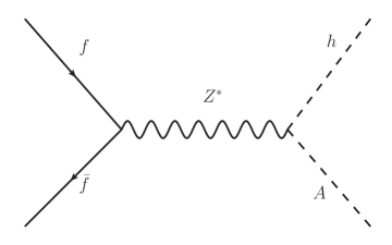
Figure 2: Associated production of $h$ and $A$.

Physical effects of antisymmetric VSS vertices have been well-studied in the literature. For example, in 2HDM, a benchmark process which embodies the effect of antisymmetric VSS vertices is

$$f+\bar{f}\rightarrow A+h$$ (75)

where $A$ and $h$ denote a generic CP-odd and CP-even 2HDM Higgs boson, respectively. The corresponding Feynman diagram is shown in Fig. 2 in unitarity gauge. Now suppose we replace the antisymmetric VSS $ZhA$ vertex in Fig. 2 by a completely symmetric VSS $ZhA$ vertex. It is obvious that if the $Z$ boson is on-shell, then the amplitude should vanish since for an on-shell massive vector-boson we have the relation $p\cdot\epsilon=0$ for its momentum and polarization vector. It is tempting to proceed with the case that $Z$ boson is off-shell. The amplitude in this case can be examined from two perspectives. First, we can perform the calculation in unitarity gauge. In this gauge, the result of dotting the $Z$ momentum $p$ at the $ZhA$ vertex into its s-channel propgator is again proportional to the $Z$ momentum $p$ at the $Zf\bar{f}$ vertex. It is then obvious that only the axial-vector part of the $Zf\bar{f}$ vertex contributes to the amplitude, with a contribution proportional to the fermion mass $m_{f}$. Alternatively, we may perform the calculation in Landau gauge ($\xi=0$), in which the diagram shown in Fig. 2 does not contribute to the amplitude, nevertheless we need to take into account the s-channel Goldstone-mediated amplitude, which again gives an contribution proportional to the fermion mass $m_{f}$.

Although usually $f$ is a light fermion with negligible mass effects, we might be interested in the case that $f$ is heavy with important mass effects, e.g. the top quark. If in this case the symmetric VSS vertex could lead to physical effects, we would seem to produce a paradox in the SLH. In the SLH there exists a symmetric $ZH\eta$ vertex, however if we consider a linearly-realized SLH as a UV completion, then it cannot lead to symmetric VSS vertices and hence there will be no related physical effects. Since the usual nonlinearly-realized SLH can be related to a linearly-realized SLH via an appropriate field redefinition, the above discussion seems to cause violation of the field redefinition invariance of the S-matrix element. We can turn the argument around to use the field redefinition invariance to infer the existence of additional contribution in the SLH which also contributes to the $f\bar{f}\rightarrow H\eta$ process such that the field redefinition invariance is maintained. In fact, if we examine the Yukawa part of the SLH Lagrangian, we would find the following four-point contact vertex ($m_{f}$ denotes the mass of $f$)

$$\mathcal{L}\supset i\frac{2\sqrt{2}g_{A}}{ft_{2\beta}}\frac{m_{f}}{v}H\eta\bar{f}\gamma^{5}f$$ (76)

Here $g_{A}$ is the axial coupling of the fermion $f$ which also appears in its interaction to $Z$ boson and the associated Goldstone $\chi$ as

$$\mathcal{L}\supset\frac{g}{2c_{W}}Z^{\mu}\bar{f}\gamma_{\mu}(g_{V}+g_{A}\gamma^{5})f+i\frac{2g_{A}m_{f}}{v}\bar{f}\gamma^{5}f\chi$$ (77)

Now if we compute the amplitude for $f\bar{f}\rightarrow H\eta$ in $R_{\xi}$ gauge, we need to include three contributions: s-channel $Z$ exchange, s-channel $\chi$ exchange, and $ffH\eta$ contact interaction, as shown in Fig. 3.

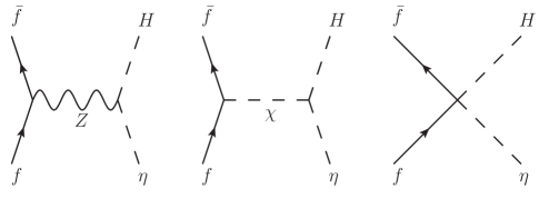
Figure 3: Feynman diagrams in the SLH for $f\bar{f}\rightarrow H\eta$ in $R_{\xi}$ gauge.

The amplitudes corresponding to these three diagrams are computed to be (from left to right):

$$i\mathcal{M}_{I} =\frac{\sqrt{2}}{vft_{2\beta}}\frac{-\xi m_{Z}^{2}}{q^{2}-\xi m_{Z}^{2}}2g_{A}m_{f}\bar{v}(p_{\bar{f}})\gamma^{5}u(p_{f})$$ (78)

$$i\mathcal{M}_{II} =\frac{\sqrt{2}}{vft_{2\beta}}\frac{q^{2}}{q^{2}-\xi m_{Z}^{2}}2g_{A}m_{f}\bar{v}(p_{\bar{f}})\gamma^{5}u(p_{f})$$ (79)

$$i\mathcal{M}_{III} =-\frac{\sqrt{2}}{vft_{2\beta}}2g_{A}m_{f}\bar{v}(p_{\bar{f}})\gamma^{5}u(p_{f})$$ (80)

Here $p_{f}$ and $p_{\bar{f}}$ are the four-momenta of $f$ and $\bar{f}$, respectively and $q\equiv p_{f}+p_{\bar{f}}$. When we add the three contributions, we find

$$i\mathcal{M}_{I}+i\mathcal{M}_{II}+i\mathcal{M}_{III}=0$$ (81)

which is exactly what we would expect from field redefinition invariance. Moreover, we see that the $Z$ and $\chi$ contributions add to be gauge-independent, while the contact interaction contribution itself is gauge-independent.

Here we would like to mention a further subtle point related to the symmetric VSS vertex. It might still be somewhat counter-intuitive the contribution from the symmetric $ZH\eta$ vertex is cancelled by the contribution from $ffH\eta$ contact vertex, since the former contribution should know the position of $Z$ pole and therefore vanish for an on-shell $Z$ boson while the latter certainly does not “feel” the $Z$ pole. To illustrate this issue, we can include the effect of $Z$ boson width $\Gamma_{Z}$ so that the $Z$ boson propagator in the unitarity gauge is written as

$$\frac{-g^{\mu\nu}+\frac{q^{\mu}q^{\nu}}{m_{Z}^{2}}}{q^{2}-m_{Z}^{2}+im_{Z}\Gamma_{Z}}$$ (82)

When this propagator is dotted into $q_{\nu}$ coming from the symmetric VSS Feynman rule, at $q^{2}=m_{Z}^{2}$ it will vanish, which seems quite plausible given our previous argument that symmetric VSS vertex does not contribute to the process in which the related vector boson is on-shell. However, this immediately leads to the paradoxical situation that near on-shell region the field redefinition invariance is again violated since the contribution from $ffH\eta$ contact vertex certainly does not know about the $Z$ pole.

The resolution of this paradox consists in the treatment of particle width in its propagator. The naive treatment in Eq. (82) is actually not quite correct and will in general lead to results that violate the Ward-Takahashi identities. A proper treatment can be made by e.g. employing the complex mass scheme which properly retains gauge invariance. The final result is, of course, no exotic structure appears near $Z$ pole and the field redefinition invariance is maintained.

IV Constraints from Electroweak Precision Observables

As discussed in Section II in the study of the pseudo-axion phenomenology there are eight sign combinations for the rotation parameters $\delta_{t},\delta_{Dd},\delta_{Ss}$. Moreover, when lepton sector is relevant, either $t_{\beta}\geq 1$ or $t_{\beta}<1$ could be possible, leading to further complication. Nevertheless, as will be shown in this section, the number of possibilities greatly reduces if we require

1. The parameter space under consideration is favored by naturalness consideration and thus embodies (to some extent) the original motivation of the SLH model.

2. The parameter space under consideration is allowed by electroweak precision measurements.

As discussed in Section II the first requirement points to the region characterized by a small top partner mass. In the SLH, currently the lower bound on top partner mass is derived from Eq. (36) where $f$ is stringently constrained by dilepton resonance searches. Constraints from direct searches for top partner production is not as competitive at the moment. For given $f$, a small top partner mass could be obtained by requiring a large $t_{\beta}$ (or $t_{\beta}^{-1}$ for $t_{\beta}<1$), which is in turn bounded by unitarity consideration. To summarize, the first requirement points to the region characterized by a small $f$ and large $t_{\beta}$ (or $t_{\beta}^{-1}$ for $t_{\beta}<1$).

As to the second requirement, in the present work we consider the following electroweak observables

1. The $W$ boson mass $m_{W}$.

2. $R$ observables measured at the $Z$-pole: $R_{b},R_{c},R_{e},R_{\mu},R_{\tau}$, which are defined by

   $$R_{b} \equiv\Gamma(b\bar{b})/\Gamma(\text{had}),R_{c}\equiv\Gamma(c\bar{c})/\Gamma(\text{had}),$$

   $$R_{l} \equiv\Gamma(\text{had})/\Gamma(l^{+}l^{-}),l=e,\mu,\tau$$ (83)

   in which $\Gamma(\text{had})$ denotes the total hadronic width of the $Z$ boson, and $\Gamma(b\bar{b}),\Gamma(c\bar{c}),\Gamma(l^{+}l^{-})$ denote the $Z$ boson partial widths into $b\bar{b},c\bar{c},l^{+}l^{-}$ channels.

To set up the calculation we choose the fine structure constant $\alpha_{\text{em}}\equiv\frac{e^{2}}{4\pi}$ (defined at $Z$-pole), Fermi constant $G_{F}$ and $Z$ boson mass $m_{Z}$ as the input parameters. Expressed with the SM quantities we have the tree level relations

$$e=g_{SM}s_{W,SM},\quad\frac{G_{F}}{\sqrt{2}}=\frac{g_{SM}^{2}}{8m_{W,SM}^{2}}$$ (84)

$$m_{Z}^{2}=\frac{g_{SM}^{2}{v_{SM}^{2}}}{4c_{W,SM}^{2}},\quad m_{W,SM}^{2}=\frac{1}{4}g_{SM}^{2}v_{SM}^{2}$$ (85)

These relations get modified in the SLH to be

$$e=gs_{W},\quad\frac{G_{F}}{\sqrt{2}}=\frac{g^{2}}{8m_{W,SLH}^{2}}\left(1-\frac{v^{2}}{4f^{2}t_{\beta}^{2}}\right)^{2}$$ (86)

$$m_{Z}^{2}=\frac{g^{2}v^{2}}{4c_{W}^{2}}+\frac{g^{2}}{32c_{W}^{2}}\left[c_{W}^{-2}(3-t_{W}^{2})-\frac{4}{3}s_{\beta}^{-2}c_{\beta}^{-2}\right]\frac{v^{4}}{f^{2}}$$ (87)

$$m_{W,SLH}^{2}=\frac{1}{4}g^{2}v^{2}+\frac{1}{24}g^{2}(3-s_{\beta}^{-2}c_{\beta}^{-2})\frac{v^{4}}{f^{2}}$$ (88)

Here we note that in the above equations, as in Section II, $g,v,s_{W}$ represent quantities in the SLH and are thus different from the SM quantities $g_{SM},v_{SM},s_{W,SM}$. From the above two set of relations we may derive

$$\frac{m_{W,SLH}^{2}}{m_{W,SM}^{2}}=1+\frac{1}{8}\left(1-t_{W,SM}^{2}+\frac{1-c_{W,SM}^{2}}{2c_{W,SM}^{2}-1}\frac{4}{t_{\beta}^{2}}\right)\frac{v_{SM}^{2}}{f^{2}}$$ (89)

$$\frac{s_{W}^{2}}{s_{W,SM}^{2}}=1-\frac{1}{8}\left(1-t_{W,SM}^{2}+\frac{c_{W,SM}^{2}}{2c_{W,SM}^{2}-1}\frac{4}{t_{\beta}^{2}}\right)\frac{v_{SM}^{2}}{f^{2}}$$ (90)

To calculate the $R$ observables in the SLH we also need the modified $Z$ couplings to light fermions. Although the corrections relative to the SM come in in the $\frac{v^{2}}{f^{2}}$ order, they are still relevant since the $R$ observables have been measured to a few per mille precision. In such a case the diagonal entries in the rotational matrices in Eq. (49) should be understood as $1-\frac{1}{2}\delta_{Dd}^{2}$ and $1-\frac{1}{2}\delta_{Ss}^{2}$, respectively. Then the modified $Z$ couplings to light fermions in the SLH can be written as

$$g^{\prime}_{L,Z,f} =g_{L,Z,f}+\delta_{Z}g_{L,Z^{\prime},f},$$

$$g^{\prime}_{R,Z,f} =g_{R,Z,f}+\delta_{Z}g_{R,Z^{\prime},f},$$

$$\text{for }f=u,c,b,e,\mu,\tau$$ (91)

In the above equations, $\delta_{Z}$ is the $\mathcal{O}\left(\frac{v^{2}}{f^{2}}\right)$ $Z-Z^{\prime}$ mixing angle, appearing in the mixing relation

$$Z^{\prime}=Z^{\prime}_{m}+\delta_{Z}Z_{m},\quad Z=Z_{m}-\delta_{Z}Z^{\prime}_{m}$$ (92)

Here $Z_{m},Z^{\prime}_{m}$ denote the final mass eigenstates after the $\mathcal{O}\left(\frac{v^{2}}{f^{2}}\right)$ rotation while $Z,Z^{\prime}$ denote the states before the $\mathcal{O}\left(\frac{v^{2}}{f^{2}}\right)$ rotation, as define via Eq. (11). In the process of gauge boson mass diagonalization, $\delta_{Z}$ is computed to be

$$\delta_{Z}=-\frac{(1-t_{W}^{2})\sqrt{3-t_{W}^{2}}}{8c_{W}}\frac{v^{2}}{f^{2}}$$ (93)

In Eq. (91), $g_{L,Z,f}=\frac{g}{c_{W}}(T_{3}^{f}-Q_{f}s_{W}^{2}),g_{R,Z,f}=-\frac{g}{c_{W}}Q_{f}s_{W}^{2}$ are leading-order coefficients of the Lagrangian terms $\bar{f}_{L}\gamma^{\mu}f_{L}Z_{\mu},\bar{f}_{R}\gamma^{\mu}f_{R}Z_{\mu}$ and $T_{3}^{f},Q_{f}$ denote the third component of the isospin and the electric charge of $f$, respectively. $g_{L,Z^{\prime},f},g_{R,Z^{\prime},f}$ are leading-order coefficients of the Lagrangian terms $\bar{f}_{L}\gamma^{\mu}f_{L}Z^{\prime}_{\mu},\bar{f}_{R}\gamma^{\mu}f_{R}Z^{\prime}_{\mu}$, which are given in Eq. (64),Eq. (65) and Eq. (66). $g^{\prime}_{L,Z,f},g^{\prime}_{R,Z,f}$ in Eq. (91) denote the coefficients of the Lagrangian terms $\bar{f}_{L}\gamma^{\mu}f_{L}Z_{\mu},\bar{f}_{R}\gamma^{\mu}f_{R}Z_{\mu}$ and $T_{3}^{f},Q_{f}$ , to the $\mathcal{O}\left(\frac{v^{2}}{f^{2}}\right)$ precision.

For $f=d$ the modified $Z$ couplings in the SLH turn out to be

$$g^{\prime}_{L,Z,d} =g_{L,Z,d}+\delta_{Z}g_{L,Z^{\prime},d}+\delta_{Dd}^{2}(g_{L,Z,D}-g_{L,Z,d}),$$

$$g^{\prime}_{R,Z,d} =g_{R,Z,d}+\delta_{Z}g_{R,Z^{\prime},d}$$ (94)

Obviously the additional correction is due to the left-handed $D-d$ mixing. The corresponding formulae for $f=s$ can be obtained by the replacement $d\rightarrow s,D\rightarrow S$. $g_{L,Z,D},g_{L,Z,S}$ are leading-order coefficients of the Lagrangian terms $\bar{D}_{L}\gamma^{\mu}D_{L}Z_{\mu},\bar{S}_{R}\gamma^{\mu}S_{R}Z_{\mu}$

$$g_{L,Z,D}=g_{L,Z,S}=\frac{1}{3}gs_{W}t_{W}$$ (95)

Now we have all the SLH couplings that are necessary to calculate the $R$ observables. It should be noted that in the above coupling formulae, $s_{W},c_{W},t_{W}$ are quantities in the SLH and are therefore different from their SM counterparts $s_{W,SM},c_{W,SM},t_{W,SM}$, see Eq. (90). Therefore, the modification of $Z$ couplings to light fermions relative to the SM is caused by three factors: $Z-Z^{\prime}$ mixing,left-handed $D-d,S-s$ mixing, and correction of the weak-mixing angle.

A $95\%$ CL level constraint can be obtained in the $f-t_{\beta}$ plane by performing a $\chi^{2}$-fit of the five $R$ observables. The $\chi^{2}$ is defined by

$$\chi^{2}=\sum_{f=b,c,e,\mu,\tau}\frac{(R_{f,SLH}-R_{f})^{2}}{\delta_{R_{f}}^{2}+\delta_{R_{f,SM}}^{2}}$$ (96)

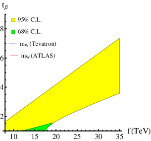
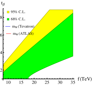
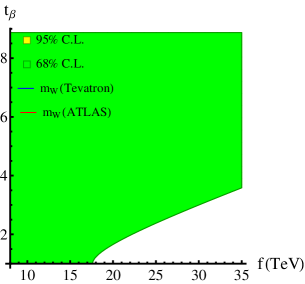
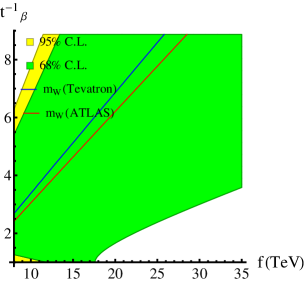
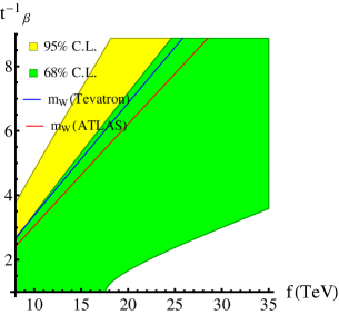
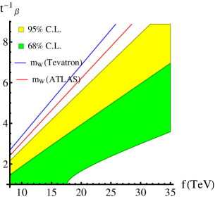
Figure 4: Constraints from $m_{W}$ and $R$ observables on the $f-t_{\beta}$ plane. Upper left: $t_{\beta}\geq 1,\delta_{Dd}^{+},\delta_{Ss}^{+}$, upper middle: $t_{\beta}\geq 1,\delta_{Dd}^{+},\delta_{Ss}^{-}$ or $t_{\beta}\geq 1,\delta_{Dd}^{-},\delta_{Ss}^{+}$, upper right: $t_{\beta}\geq 1,\delta_{Dd}^{-},\delta_{Ss}^{-}$, lower left: $t_{\beta}\leq 1,\delta_{Dd}^{+},\delta_{Ss}^{+}$, lower middle: $t_{\beta}\leq 1,\delta_{Dd}^{+},\delta_{Ss}^{-}$ or $t_{\beta}\geq 1,\delta_{Dd}^{-},\delta_{Ss}^{+}$, lower right: $t_{\beta}\leq 1,\delta_{Dd}^{-},\delta_{Ss}^{-}$. See the text for detailed description.

In the above equation, $R_{f}$ denote the experimental values and $\delta_{R_{f}}$ denotes the associated experimental uncertainty. Also, $R_{f,SM}$ is the SM theory prediction and $\delta_{R_{f,SM}}$ denotes the associated theory uncertainty. Their values are listed in Table  1 Erler:2018rpp .

Quantity	Value	Standard Model
$R_{e}$	$20.804\pm 0.050$	$20.737\pm 0.010$
$R_{\mu}$	$20.785\pm 0.033$	$20.737\pm 0.010$
$R_{\tau}$	$20.764\pm 0.045$	$20.782\pm 0.010$
$R_{b}$	$0.21629\pm 0.00066$	$0.21582\pm 0.00002$
$R_{c}$	$0.1721\pm 0.0030$	$0.17221\pm 0.00003$

Table 1: Experimental values and the SM predictions of the $R$ observables.

As to the constraint from $W$ boson mass, we treat it separately and consider two most precise measurements Erler:2018rpp

$$m_{W} =80.387\pm 0.016~{}{\mbox{GeV}}\quad\text{(Tevatron)}$$ (97)

$$m_{W} =80.370\pm 0.019~{}{\mbox{GeV}}\quad\text{(ATLAS)}$$ (98)

while we note the SM prediction for $m_{W}$ is Erler:2018rpp

$$m_{W,SM}=80.358\pm 0.004~{}{\mbox{GeV}}$$ (99)

In Figure 4 the results of the electroweak precision analysis of $m_{W}$ and $R$ observables are shown. To clarify the situation we present the results according to whether $t_{\beta}\geq 1$ and the sign combination of the rotation parameters $\delta_{Dd},\delta_{Ss}$ (see Eq. (53)). At first sight there are eight possibilities in total, however it is immediately recognized that $\delta_{Dd}^{+},\delta_{Ss}^{-}$ and $\delta_{Dd}^{-},\delta_{Ss}^{+}$ make no difference in terms of constraints in the $f-t_{\beta}$ plane, reducing the number of possibilities to six. Therefore we obtain the six panels in Figure 4, each panel showing one possibility as described in the caption.

For all the panels, the green and yellow regions correspond to parameter points that are allowed by $\chi^{2}$-fit of $R$ observables at $68\%$ and $95\%$ CL, respectively. These allowed regions do not exhibit a $t_{\beta}\rightarrow t_{\beta}^{-1}$ symmetry (for example, the allowed region in the upper right panel and the lower left panel still differ under the transformation $t_{\beta}\rightarrow t_{\beta}^{-1}$), since in the computation of $R$ observables, the correction of $s_{W}^{2}$ relative to its SM value has to be taken into account, as was pointed out previously. When $f$ is larger than about $17~{}{\mbox{TeV}}$ there will be a lower theoretical bound (from the mass relation) on $t_{\beta}$ or $t_{\beta}^{-1}$ which is larger than $1$, corresponding to the white region at large $f$ and small $t_{\beta}$ or $t_{\beta}^{-1}$ in each panel. The $2\sigma$ constraints from $m_{W}$ measurements are simply implemented by requiring

$$|m_{W,SLH}-m_{W}|<2\sqrt{\delta_{m_{W}}^{2}+\delta_{m_{W,SM}}^{2}}$$ (100)

In the above equation $m_{W}$ denotes the experimentally measured $W$ boson mass and $\delta_{m_{W}}$ and $\delta_{m_{W,SM}}$ denote the associated experimental and theoretical uncertainties, respectively. We superimpose the constraint boundary on the six plots as blue or red lines, representing constraints from Tevatron or ATLAS measurements, respectively. For all these $m_{W}$ constraint boundary lines, the regions on the right side of the lines are allowed at $2\sigma$ level.

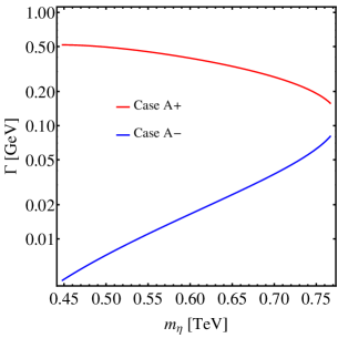
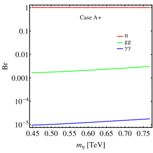
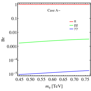
Figure 5: Total width $\Gamma$ and decay branching ratios of $\eta$ in Case A.

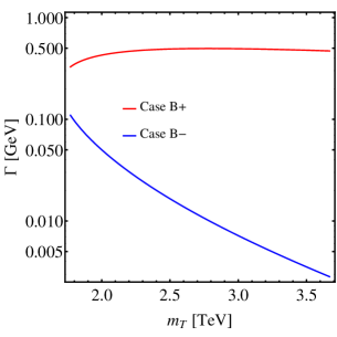
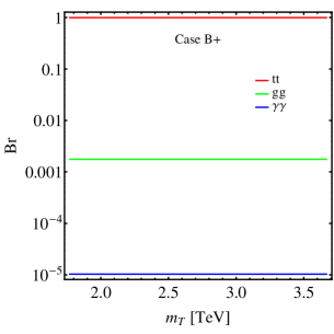
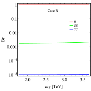
Figure 6: Total width $\Gamma$ and decay branching ratios of $\eta$ in Case B.

As can be seen from Figure 4, if $t_{\beta}<1$, then the region favored by naturalness consideration is disfavored by constraints from both $R$ observables and $W$ boson mass measurements, regardless of the sign combination of the rotation parameters $\delta_{Dd},\delta_{Ss}$. If $t_{\beta}\geq 1$, then $W$ boson mass measurement does not constrain the parameter region favored by naturalness consideration. However, in this case constraints from $R$ observables are significant when any of the rotation parameters $\delta_{Dd},\delta_{Ss}$ adopt the plus sign in Eq. (53). This is because the choice of plus sign leads to a large $t_{\beta}$ enhancement of the rotation parameter and therefore a larger deviation of $Z$ couplings to the corresponding fermion. Although the lower bound on $f$ has been pushed to around $7.5~{}{\mbox{TeV}}$ by LHC dilepton resonance searches, the $R$ observable constraints still force us to avoid this $t_{\beta}$ enhancement, and consequently the only possibility left is $\delta_{Dd}^{-},\delta_{Ss}^{-}$ with $t_{\beta}\geq 1$. This result has important consequences for the pseudo-axion phenomenology since the sign combinations of $\delta_{Dd},\delta_{Ss}$ will determine how $\eta$ interacts with the $D,S$ quarks which in turn influences the decay and production of the $\eta$ particle, as will be discussed in more detail in the next section.

In previous literature on the SLH model the $t_{\beta}\geq 1$ and $t_{\beta}<1$ cases are usually not distinguished, since a $t_{\beta}\rightarrow t_{\beta}^{-1}$ symmetry is tacitly assumed. Then only the $t_{\beta}\geq 1$ case is considered. However strictly speaking this symmetry is only valid when the leptonic sector is not considered. Here we established clearly that if we consider the region favored by naturalness consideration, the $t_{\beta}<1$ case is disfavored by measurements $m_{W}$ and $R$ observables. This is closely related to the breakdown of the $t_{\beta}\rightarrow t_{\beta}^{-1}$ symmetry in the lepton sector. Moreover, in previous literature Han:2005ru ; Reuter:2012sd , the sign combination of the rotation parameter $\delta_{Dd},\delta_{Ss}$ was simply assumed to be (effectively) $\delta_{Dd}^{-},\delta_{Ss}^{-}$, in order to suppress contribution to the electroweak precision observables. Here we also establish firmly this choice based on constraints from $R$ observables, combined with $m_{W}$ and naturaless consideration, keeping in mind that the constraint on $f$ has been pushed to around $7.5~{}{\mbox{TeV}}$ due to updated LHC constraints.

V Production and Decay of the Pseudo-Axion

With the preparation made in the previous three sections we are now ready to calculate the production and decay of the pseudo-axion. We will restrict ourselves to the region $2m_{t}\lesssim m_{\eta}\lesssim 1~{}{\mbox{TeV}}$, which is favored by naturalness consideration. All the related partial widths formulae are given in Appendix B.

V.1 Decay of the Pseudo-Axion

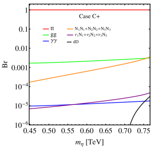
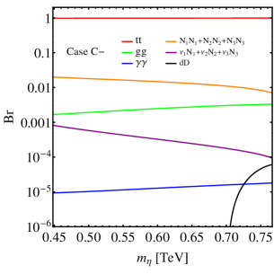
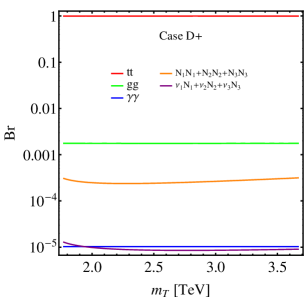
Figure 7: Decay branching ratios of $\eta$ in Case C and Case D.

For $\eta$ in the mass range $2m_{t}\lesssim m_{\eta}\lesssim 1~{}{\mbox{TeV}}$, it can always decay into $t\bar{t},gg,\gamma\gamma$ channels. (The $WW,ZZ,Z\gamma$ channels are also possible and may have comparable branching ratio compared to $\gamma\gamma$. However from a detection viewpoint, it is preferrable to consider further decays into leptons in these channels, leading to an additional suppression by the leptonic branching. For simplicity we will not consider these channels further in this work.). $\eta\rightarrow ZH$ is highly suppressed, since the antisymmetric $ZH\eta$ vertex is suppressed to $\mathcal{O}\left(\frac{v^{3}}{f^{3}}\right)$ while the symmetric $ZH\eta$ vertex does not contribute, as pointed out in Section III. If the new fermions $D,S,N$ are heavy enough such that they cannot appear as decay products of $\eta$, then we are left with only the $t\bar{t},gg,\gamma\gamma$ channels. Nevertheless we should keep in mind that when $f$ and $m_{\eta}$ are given, the partial withds of these channels still depend on the masses of the additional heavy quarks $T,D,S$ which do not appear as decay products of $\eta$. First, the $\eta\rightarrow t\bar{t}$ decay is controlled by the rotation parameter $\delta_{t}$, which in turn depends on the top partner mass. The loop-induced decays $\eta\rightarrow gg,\gamma\gamma$ have contributions from both the top quark and the heavy quark partners $T,D,S$. The top quark contribution again depends on $\delta_{t}$ while the $T,D,S$ contributions depend on the $\eta T\bar{T},\eta D\bar{D},\eta S\bar{S}$ couplings which are propotional to the corresponding rotation parameters times the quark partner mass. Experimentally the current lower bound for light-flavor quark partner $D$ and $S$ is around $700~{}{\mbox{GeV}}$ Sirunyan:2017lzl . Thus for a heavy enough $\eta$ the $\eta\rightarrow Dd,Ss$ channels are still possible if the mass of $D$ or $S$ is close to the lower bound. To be definite, we will consider four benchmark scenarios:

1. Case A: $f=8~{}{\mbox{TeV}},m_{T}=m_{D}=m_{S}=3~{}{\mbox{TeV}},\text{all }m_{N}>m_{\eta}$.

2. Case B: $f=8~{}{\mbox{TeV}},m_{\eta}=500~{}{\mbox{GeV}},m_{D}=m_{S}=m_{T},\text{all }m_{N}>m_{\eta}$.

3. Case C: $f=8~{}{\mbox{TeV}},m_{T}=3~{}{\mbox{TeV}},m_{D}=700~{}{\mbox{GeV}},m_{S}=1~{}{\mbox{TeV}},\text{all }m_{N}=150~{}{\mbox{GeV}}$.

4. Case D: $f=8~{}{\mbox{TeV}},m_{\eta}=500~{}{\mbox{GeV}},m_{D}=m_{S}=m_{T},\text{all }m_{N}=150~{}{\mbox{GeV}}$.

For each case, there are two allowed sign combinations for the rotation parameters $(\delta_{t},\delta_{Dd},\delta_{Ss})$: $(+,-,-)$ and $(-,-,-)$. Other choices are excluded by electroweak precision measurements, if we are only interested in parameter region favored by nartualness consideration. Therefore in the following we will use Case A$+$, Case A$-$, etc. to indicate the sign choice of $\delta_{t}$ in each case (see Eq. (52)).

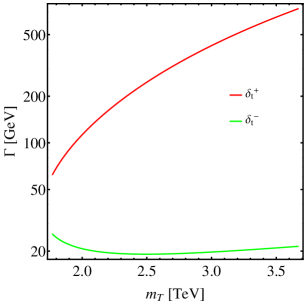
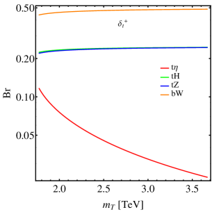
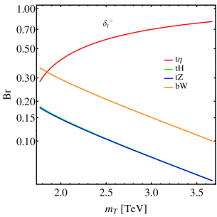
Figure 8: Total width $\Gamma$ and decay branching ratios of $T$ in the SLH. We assume $f=8~{}{\mbox{TeV}}$ and $m_{\eta}=500~{}{\mbox{GeV}}$. Note that in the considered mass range $T\rightarrow bX,tY$ channels do not open.

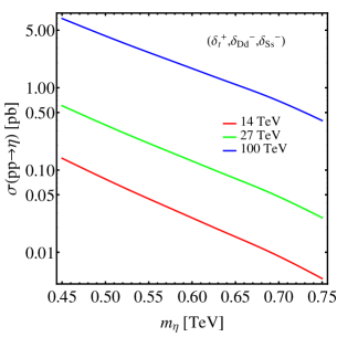
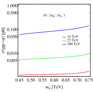
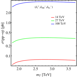
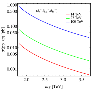
Figure 9: Gluon fusion production cross section of $\eta$ as a function of $m_{\eta}$ (upper panel, assuming $m_{T}=m_{D}=m_{S}=3~{}{\mbox{TeV}}$) or $m_{T}$ (lower panel, assuming $m_{D}=m_{S}=m_{T}$ and $m_{\eta}=500~{}{\mbox{GeV}}$). The sign combination of $(\delta_{t},\delta_{Dd},\delta_{Ss})$ is indicated in each plot.

The total width and branching ratios of $\eta$ are shown in Figure 5 and Figure 6 for Case A and Case B respectively. In these two cases, the additional fermion partners $D,S,N$ are not light enough to appear as decay products of $\eta$ and therefore we are left with the standard $\eta\rightarrow t\bar{t},gg,\gamma\gamma$ channels. From the figures it is clear that $\eta$ can be viewed as a narrow width particle, however the width is not small enough to give rise to displaced vertices. In both Case A and Case B and for both sign choices, $\eta$ decays almost $100\%$ to $t\bar{t}$, with only very small branching ratios to $gg$ ($\mathcal{O}(0.1\%)$) and $\gamma\gamma$ ($\mathcal{O}(0.001\%)$). Here (and in the following) all the partial widths are calculated at LO, but it is obvious that the inclusion of higher order radiative corrections has little effect on the whole picture. From a detection point of view this situation is somewhat unfortunate since the dominant channel $t\bar{t}$ suffer from huge background at hadron colliders, while the clean channel $\gamma\gamma$ has an extremely small branching ratio. It is natural to ask how the situation will change if any of $D,S,N$ is light enough, such that exotic channels like $\eta\rightarrow NN,N\nu,Dd,Ss$ could be open. This is embodied in Cases C and D and we show the corresponding branching ratio plots in Figure 7. Nevertheless the exotic channels contribute at most a few percent in terms of branching ratio, therefore are of little use for $\eta$ detection even if any of $D,S,N$ is light enough. This can be understood from the interaction Lagrangian containing the $\eta Dd,\eta Ss$ and $\eta N\nu,\eta NN$ vertices. The $\eta Dd$ vertex is shown in Eq. (62). When $\eta\rightarrow Dd$ is open, $\frac{M_{D}}{v}$ is an $\mathcal{O}(1)$ quantity, and therefore from Eq. (62) we may recognize that the $\eta Dd$ coupling can be considered as being relatively suppressed by $\mathcal{O}(\frac{v}{f})$ compared to $\eta t\bar{t}$ vertex. This leads to the suppression of $\eta\rightarrow Dd$ channel. The $\eta N\nu$ coupling is relatively suppressed by $\mathcal{O}(\frac{v}{f})$ compared to $\eta NN$ coupling, as can be seen from Eq. (60). However, when $\eta\rightarrow NN$ is open, $M_{Nn}$ can be at most $\mathcal{O}(v)$. Moreover, the $\eta NN$ coupling suffers from a $t_{\beta}$ suppression. Therefore numerically $\eta\rightarrow NN$ channel is much suppressed compared to $\eta\rightarrow t\bar{t}$ channel.

V.2 Decay of the Top Partner

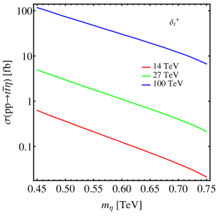
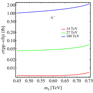
Figure 10: Production cross section of $pp\rightarrow t\bar{t}\eta$ as a function of $m_{\eta}$. We assume $f=8~{}{\mbox{TeV}}$ and $m_{T}=3~{}{\mbox{TeV}}$.

The pseudo-axion may appear as a decay product of some additional heavy particles in the model. Among the additional particles in the SLH only $Z^{\prime}$ and $T$ are closely related to EWSB and naturalness favors small $Z^{\prime}$ and $T$ masses within theoretical constraints. In this subsection we consider the decay of the top partner. The possibility of $T\rightarrow t+a$ where $T$ and $a$ denote the top partner and a pNGB in the context of composite Higgs models have been investigated in the literature Bizot:2018tds ; Serra:2015xfa ; Kearney:2013cca . Here we focus on the situation in the SLH. To be specific we fix $f=8~{}{\mbox{TeV}}$ and $m_{\eta}=500~{}{\mbox{GeV}}$ and then plot the total width and branching ratios of $T$ as a function of the top partner mass $m_{T}$ in Figure 8. Both $\delta_{t}^{+}$ and $\delta_{t}^{-}$ possibilities are considered. Note that when $m_{T}$ is also given, then according to the mass relation, $t_{\beta}$ can be calculated, which in turn determines the total width and branching ratios. The relation ${\mathrm{Br}}(T\rightarrow bW)=2{\mathrm{Br}}(T\rightarrow tH)=2{\mathrm{Br}}(T\rightarrow tZ)$ holds to a good approximation. In the $\delta_{t}^{+}$ case, ${\mathrm{Br}}(T\rightarrow t\eta)$ is small (not larger than $10\%$ for $m_{T}>2~{}{\mbox{TeV}}$) and decreases with the increase of $m_{T}$. In the $\delta_{t}^{-}$ case, ${\mathrm{Br}}(T\rightarrow t\eta)$ is sizable and becomes dominant (larger than $50\%$) for $m_{T}\gtrsim 2.2~{}{\mbox{TeV}}$. Another interesting and important feature is about the total width of $T$. In the $\delta_{t}^{-}$ case, the total width is around $20~{}{\mbox{GeV}}$ which makes the narrow width approximation valid to high precision. In the $\delta_{t}^{+}$ case, the total width increases with $m_{T}$. For $m_{T}\approx 3.5~{}{\mbox{TeV}}$ the total width increases to around $500~{}{\mbox{GeV}}$. In this case $\Gamma/M\lesssim 20\%$ and the narrow width approximation still roughly holds, if the phase space is large enough. The width will however leave appreciable impact on the invariant mass distribution of the $T$ decay products.

V.3 Direct Production of the Pseudo-Axion

The pseudo-axion can be directly produced via the gluon fusion mechanism at hadron colliders. The particles running in the loop now contain $t,T,D,S$. In the calculation of the production cross section, we consider the $14~{}{\mbox{TeV}}$ (HL-)LHC, the $27~{}{\mbox{TeV}}$ HE-LHC and also the $100~{}{\mbox{TeV}}$ FCC-hh. The production cross sections are plotted in Figure 9 as a function of $m_{\eta}$ or $m_{T}$, with other parameters described in the figure caption. Although the production cross section may reach $\mathcal{O}(\text{pb})$ in certain region of parameter space, unfortunately when combined with $\eta$ decay it turns out very difficult to detect in the gluon fusion channel. The dominant $t\bar{t}$ decay mode suffers from huge background, while the $\gamma\gamma$ decay mode has only $\mathcal{O}(10^{-5})$ branching ratio.

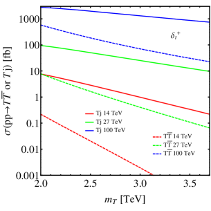
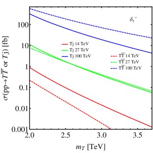
Figure 11: Production cross section of $pp\rightarrow T\bar{T}$ and $pp\rightarrow Tj$ as a function of $m_{T}$. We assume $f=8~{}{\mbox{TeV}}$ and $m_{\eta}=500~{}{\mbox{GeV}}$. For $pp\rightarrow Tj$, the contribution from $pp\rightarrow\bar{T}j$ is also included.

Another way to directly produce $\eta$ is through the $pp\rightarrow t\bar{t}\eta$ channel. We plot the production cross section as a function of $m_{\eta}$ in Figure 10, for three center of mass energies and both $\delta_{t}^{+}$ and $\delta_{t}^{-}$. Here we fix $f=8~{}{\mbox{TeV}}$ and $m_{T}=3~{}{\mbox{TeV}}$, and therefore for given $m_{\eta}$, $t_{\beta}$ (and $\delta_{t}^{\pm}$)is also determined. The cross section in the $\delta_{t}^{-}$ case is much smaller than that of the $\delta_{t}^{+}$ case. Even in the $\delta_{t}^{+}$ case the detection of $pp\rightarrow t\bar{t}\eta$ process is still very difficult. For instance, if we take $m_{\eta}=450~{}{\mbox{GeV}}$, then in the $\delta_{t}^{+}$ case the cross section reaches only about $0.6~{}{\mbox{fb}}$ at $14~{}{\mbox{TeV}}$ and $100~{}{\mbox{fb}}$ at $100~{}{\mbox{TeV}}$. When we consider $\eta\rightarrow t\bar{t}$ decay, there exists the SM four-top production as an irreducible background, with cross section of about $10~{}{\mbox{fb}}$ at $14~{}{\mbox{TeV}}$ and $5000~{}{\mbox{fb}}$ at $100~{}{\mbox{TeV}}$. Unfortunately, since $m_{\eta}$ is not far above the $2m_{t}$ threshold, we don’t expect large differences of kinematical features between the $pp\rightarrow t\bar{t}\eta$ signal and the SM four-top background, making the discrimination very difficult. With larger $m_{\eta}$ (say $1~{}{\mbox{TeV}}$), the top pair from $\eta$ decay can be boosted, with invariant mass distribution peaked around a high value, which can facilitate the discrimination from SM backgrounds. However, the cross section for such a heavy $\eta$ becomes very small. Therefore we don’t expect $pp\rightarrow t\bar{t}\eta$ to be a promising channel for future $\eta$ detection in the SLH.

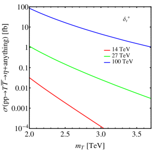
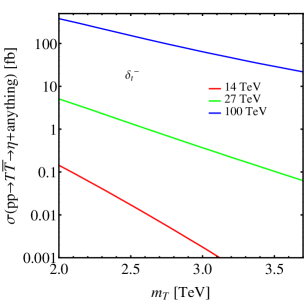
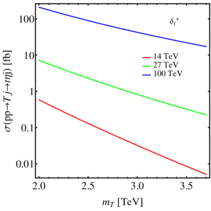
Figure 12: Cross section of $pp\rightarrow T\bar{T}\rightarrow\eta+\text{anything}$ and $pp\rightarrow Tj\rightarrow\eta+\text{anything}$ as a function of $m_{T}$. We assume $f=8~{}{\mbox{TeV}}$ and $m_{\eta}=500~{}{\mbox{GeV}}$. For $pp\rightarrow Tj$, the contribution from $pp\rightarrow\bar{T}j$ is also included.

V.4 Pseudo-Axion Production from Top Partner Decay

The above discussion shows that it is very difficult to detect $\eta$ via the gluon fusion and $t\bar{t}\eta$ associated production channels. It is therefore natural to consider alternative $\eta$ production mechanisms, such as decay from heavier particles. In the SLH, particles that can be heavier than $\eta$ are $T,D,S,N,Z^{\prime},X$ and $Y$. Here we will concentrate on $T$, which is most tightly connected to EWSB. We will briefly comment on the possibility of detecting $\eta$ from other heavy particle decays in the next subsection.

Under current constraints, the lower bound on $m_{T}$ is already larger than the largest possible value of $m_{\eta}$ plus $m_{t}$, therefore the exotic decay channel $T\rightarrow t\eta$ will always open. The branching fraction of $T\rightarrow t\eta$ has been discussed (see Figure 8). Here we focus on top partner production. Two major production mechanisms are pair production through QCD interaction, and single production through the $TbW$ vertex. Pair production has the virtue of being model-independent, while single production depends on the value of $\delta_{t}$. In Figure 11 we present the cross section of $pp\rightarrow T\bar{T}$ and $pp\rightarrow Tj+\bar{T}j$ for both $\delta_{t}^{+}$ and $\delta_{t}^{-}$, as a function of $m_{T}$ while we fix $f=8~{}{\mbox{TeV}},m_{\eta}=500~{}{\mbox{GeV}}$. Three center of mass energies ($14,27,100~{}{\mbox{TeV}}$) are considered. Whether pair or single production delivers a larger cross section depends on the sign choice for $\delta_{t}$ and the center of mass energy. In the $\delta_{t}^{+}$ case, for all three center of mass energies the single production cross section is larger. In the $\delta_{t}^{-}$ case, at $14~{}{\mbox{TeV}}$ single production is larger since pair production is highly suppressed by phase space. At $27~{}{\mbox{TeV}}$ pair production and single production become comparable while for $100~{}{\mbox{TeV}}$ collider energy pair production dominates.

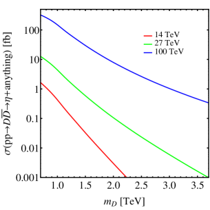
Figure 13: Production cross section of $pp\rightarrow D\bar{D}\rightarrow\eta+\text{anything}$ as a function of $m_{D}$ (left) and $m_{\eta}$ (right). For the left plot, we assume $f=8~{}{\mbox{TeV}},m_{T}=3~{}{\mbox{TeV}},m_{\eta}=500~{}{\mbox{GeV}}$. For the right plot, we assume $f=8~{}{\mbox{TeV}},m_{T}=3~{}{\mbox{TeV}},m_{D}=700~{}{\mbox{GeV}}$.

To detect $\eta$ we would also like to consider the top partner decay $T\rightarrow t\eta$ that follows the pair or single production of $T$. The associated cross sections are plotted as a function of $m_{T}$ in Figure 12, using narrow width approximation, for both $\delta_{t}^{+}$ and $\delta_{t}^{-}$. For definiteness we take $f=8~{}{\mbox{TeV}},m_{\eta}=500~{}{\mbox{GeV}}$. To be precise, the plotted cross sections are defined by (for $pp\rightarrow Tj$, the contribution from $pp\rightarrow\bar{T}j$ is also included)

$$\sigma(pp\rightarrow Tj\rightarrow\eta+\text{anything}) =\sigma(pp\rightarrow Tj)\times{\mathrm{Br}}(T\rightarrow t\eta)$$ (101)

$$\sigma(pp\rightarrow T\bar{T}\rightarrow\eta+\text{anything}) =2\sigma(pp\rightarrow T\bar{T})\times{\mathrm{Br}}(T\rightarrow t\eta)(1-{\mathrm{Br}}(T\rightarrow t\eta))$$

$$+\sigma(pp\rightarrow T\bar{T})\times{\mathrm{Br}}^{2}(T\rightarrow t\eta)$$ (102)

For the purpose of $\eta$ detection, let us consider using the $\eta\rightarrow t\bar{t}$ channel, which has almost $100\%$ branching fraction. Then the $\eta$ production from top partner decays generically leads to a multi-top ($\geq 3$) signature. Moreover, the top quarks will be boosted since $m_{T}\gg m_{t}+m_{\eta}$. For example, suppose a $2~{}{\mbox{TeV}}$ top partner is produced with little boost in the lab frame and then decays into $t+\eta$. At this step $t$ and $\eta$ roughly shares the rest energy of the top partner and therefore will each have about $1~{}{\mbox{TeV}}$ energy. The $\eta$ boson then further decays into $t$ and $\bar{t}$, each of which roughly has an energy about $0.5~{}{\mbox{TeV}}$. All three top quarks are boosted: the first one will have the decay ($t\rightarrow bW$) cone size approximated by $\sim 2m_{t}/E_{t}\simeq 0.4$ while the second and third top have $\sim 2m_{t}/E_{t}\simeq 0.8$. Furthermore, the second and the third top quark decaying from $\eta$ is close to each other, of separation approximated by $\sim 2m_{\eta}/E_{\eta}\simeq 0.8$.

In the single production case, the signature will be $3t+j$, in which the first top is highly boosted while the second and third are still somewhat boosted and close to each other. One can make use of such kinematics to discriminate from QCD backgrounds. The most serious background is perhaps multi-top production. One may be able to reduce the background using the boosted techniques Kaplan:2008ie . In the pair production case, if we consider one top partner decaying into $t\eta$ with the other decaying into $bW$, then we obtain a signature of $3t+b+W$ in which the top quarks and also the $W$ boson will be boosted. In both single and pair production channels, the invariant mass peaks at $m_{T}$ and $m_{\eta}$ will also be helpful in discriminating between the signal and background. Nevertheless, a full signal-background analysis using boosted-top techniques is beyond the scope of the present work.

From Figure 12, we see that the cross sections at $14~{}{\mbox{TeV}}$ (HL-)LHC for all these channels are very small ($<1~{}{\mbox{fb}}$), making the detection very difficult. Nevertheless, with the increase of collider energy, the signal cross sections increase significantly. For example, at the $100~{}{\mbox{TeV}}$ FCC-hh, for both $\delta_{t}^{+}$ and $\delta_{t}^{-}$ and pair and single production channels, at relatively small $m_{T}$ the cross sections could reach $\mathcal{O}(100~{}{\mbox{fb}})$. In the $\delta_{t}^{+}$ case, the single production (with the top partner decaying to $t\eta$) turns out to deliver a cross section of about $200~{}{\mbox{fb}}$, which is larger than the pair production channel. In the $\delta_{t}^{-}$ case, the pair production (with one top partner decaying to $t\eta$) turns out to deliver a cross section of about $400~{}{\mbox{fb}}$, which is however larger than the single production channel.

In principle, top partner production and decay provide a way to measure $t_{\beta}$ (which is important for testing the SLH mass relation) and also discriminate between the $\delta_{t}^{+}$ and $\delta_{t}^{-}$ cases. In practice, we may consider the partial width ratio $R_{\eta}\equiv\frac{\Gamma(T\rightarrow t\eta)}{\Gamma(T\rightarrow bW)}$ as both an indicator of the sign choice for $\delta_{t}$ and a way to measure $\delta_{t}$, which in turn determines $t_{\beta}$. $\delta_{t}$ can also be determined from $pp\rightarrow Tj$ production since the cross section is proportional to $\delta_{t}^{2}$. Furthermore, in the $\delta_{t}^{+}$ case the total width of $T$ could reach $\mathcal{O}(100~{}{\mbox{GeV}})$, which may have impact on the invariant mass distribution of $T$ decay products (e.g. $bW$). Measurement of the $T$ total width in principle could also help determine the value of $\delta_{t}$. If $\delta_{t}$ is determined (including the sign choice), we should note however the determination of $t_{\beta}$ and the test of mass relation still requires the measurement of $f$ and $m_{\eta}$, which can be obtained if we are able to measure the masses of $Z^{\prime}$ and $\eta$ particles.

V.5 Comments on Other Channels

Currently the SLH is stringently constrained by the LHC $Z^{\prime}\rightarrow ll$ search, nevertheless it also means that if the SLH was realized in nature, the $Z^{\prime}\rightarrow ll$ signature would be the first place that we might expect the appearance of new physics. Then it would also be important to consider whether we may detect $\eta$ as a decay product of $Z^{\prime}$. Two channels might be conceived: $Z^{\prime}\rightarrow\eta H$ and $Z^{\prime}\rightarrow\eta Y$. However, it turns out they give too small branching fractions: ${\mathrm{Br}}(Z^{\prime}\rightarrow\eta H)<0.01$ and ${\mathrm{Br}}(Z^{\prime}\rightarrow\eta Y)<10^{-4}$. This is regardless of whether the $Z^{\prime}\rightarrow DD,SS,NN$ channels are kinematically allowed. Therefore it is not preferable to consider detecting $\eta$ from $Z^{\prime}$ decay.

If kinematically allowed, we might also consider $D\rightarrow d\eta,S\rightarrow s\eta,N\rightarrow\nu\eta$ decays. However, these decay channels also suffer from small branching fractions, since the $\eta Dd,\eta Ss,\eta N\nu$ couplings are $\mathcal{O}(\frac{v}{f})$ suppressed compared to $HDd,HSs,HN\nu$ couplings (see Eq. (60) and Eq. (62)). For example, $D$ will dominantly decay to $uW,dZ,dH$, with only ${\mathrm{Br}}(D\rightarrow d\eta)<1\%$, for the benchmark point $f=8~{}{\mbox{TeV}},m_{T}=2~{}{\mbox{TeV}},m_{\eta}=0.5~{}{\mbox{TeV}}$ and any value of $m_{D}$. Here $\delta_{Dd}^{-}$ is assumed, to be consistent with electroweak precision constraints. As to $D$ production, for the $\delta_{Dd}^{-}$ case, there is a $t_{\beta}^{-1}$ suppresion for single $D$ production, therefore $D$ pair production is more promising. Moreover, current collider constraint on $D$ mass is not stringent, such that $m_{D}=700~{}{\mbox{GeV}}$ is still allowed Sirunyan:2017lzl . Therefore, if $m_{D}$ is as light as $700~{}{\mbox{GeV}}$, the large $pp\rightarrow D\bar{D}$ production cross section could compensate for the small $D\rightarrow d\eta$ branching fraction, leading to sizable $\eta$ production rate. At the $100~{}{\mbox{TeV}}$ FCC-hh, the $\eta$ production cross section from $D$ decay, $\sigma(pp\rightarrow D\bar{D}\rightarrow\eta+\text{anything})$ could also reach more than $100~{}{\mbox{fb}}$ for $m_{D}$ not much larger than $700~{}{\mbox{GeV}}$(see Figure 13). This is comparable with $\eta$ cross section from top partner production, and in principle could also be used to measure $t_{\beta}$. The expected signature would be $t\bar{t}+2j+W/Z/H$, in which the $W/Z/H$ should be boosted. The existence of various intermediate resonances would be helpful in discriminating signal and background. Nevertheless, we should be aware that naturalness does not offer any guidance on the preferred value of $m_{D}$. This is different from the case of $m_{T}$, in which naturalness clearly favors a lighter top partner. The case of $pp\rightarrow S\bar{S}$ production with $S\rightarrow s\eta$ decay is completely similar to the above discussion of $D$ production and decay. For $N$, $Br(N\rightarrow\nu\eta)$ is also very small (less than $1\%$ for the benchmark point $f=8~{}{\mbox{TeV}},m_{T}=2~{}{\mbox{TeV}},m_{\eta}=0.5~{}{\mbox{TeV}}$ and any value of $m_{N}$. Moreover, $N$ does not have QCD pair production channels like $D,S$, therefore it is difficult to detect $\eta$ from $N$ decay at hadron colliders.

The $X,Y$ gauge bosons in the SLH may have decays like $X\rightarrow\eta W$ and $Y\rightarrow H\eta$. However, single production cross section of $X,Y$ at hadron colliders are highly suppressed, and we need to rely on production with other heavy particles (heavy gauge bosons or quark partners) Han:2005ru . Since $X,Y$ bosons are quite heavy (with masses of about $0.8m_{Z^{\prime}}$), their production with other heavy particles would be limited by phase space while their decays are expected to be dominated by fermionic final states. Therefore we don’t consider $\eta$ production from $X,Y$ decays as promising channels for $\eta$ detection.

VI Discussion and Conclusions

Channel	Cross section at the benchmark point ($\sqrt{s}=100~{}{\mbox{TeV}}$)(fb)	Signature
$pp\rightarrow T\bar{T}\rightarrow\eta+\text{anything}$	$84(\delta_{t}^{+}),\quad\quad 379(\delta_{t}^{-})$	$3t+W+b$ or $4t+Z/H$
$pp\rightarrow Tj\rightarrow\eta+\text{anything}$	$209(\delta_{t}^{+}),\quad\quad 133(\delta_{t}^{-})$	$3t+j$
$pp\rightarrow D\bar{D}\rightarrow\eta+\text{anything}$	322	$2t+W/Z/H+2j$

Table 2: Summary of $\eta$ production from $T,D(S)$ decays at the $100~{}{\mbox{TeV}}$ FCC-hh. For $pp\rightarrow Tj$, the contribution from $pp\rightarrow\bar{T}j$ is also taken into account. For $T\bar{T},Tj$ channels, the benchmark point is $f=8~{}{\mbox{TeV}},m_{T}=2~{}{\mbox{TeV}},m_{\eta}=500~{}{\mbox{GeV}}$ while for $D\bar{D}$ channels, the benchmark point is $f=8~{}{\mbox{TeV}},m_{T}=3~{}{\mbox{TeV}},m_{\eta}=500~{}{\mbox{GeV}},m_{D}=700~{}{\mbox{GeV}}$. When listing the signatures for $T\bar{T},D\bar{D}$ channels we don’t consider the situation in which both quark partners decay into $\eta+t$ or $\eta+j$, but this possibility is taken into account in the cross section values and plots.

The Simplest Little Higgs model provides a most simple manner to concretely realize the collective symmetry breaking mechanism, in order to alleviate the Higgs mass naturalness problem. In the scalar sector, its particle content is very economical, since besides the CP-even Higgs which should serve as the $125~{}{\mbox{GeV}}$ Higgs-like particle, the only additional scalar particle is the pseudo-Nambu-Goldstone particle $\eta$ associated with a remnant global $U(1)$ symmetry. The detection of $\eta$ is important since its mass enters into the crucial SLH mass relation and it will also play an important role in discriminating SLH from other new physics scenarios. In this work we are concerned with the production and decay of $\eta$ particle at future hadron colliders. We found that for natural region of parameter space, $m_{\eta}$ is larger than $2m_{t}$ and decays almost exclusively to $t\bar{t}$, and ${\mathrm{Br}}(\eta\rightarrow\gamma\gamma)$ is too small to be considered promising for detection. Also it is very difficult to detect $\eta$ in direct production channels $pp\rightarrow\eta$ (gluon fusion) and $pp\rightarrow t\bar{t}\eta$. Channels that are worth further consideration include $\eta$ production from heavy quark partner ($T,D,S$) decays, in which the heavy quark partner might be singly (for $T$) or pair produced. The corresponding $\eta$ production cross section at $100~{}{\mbox{TeV}}$ FCC-hh could reach $\mathcal{O}(100~{}{\mbox{fb}})$ for certain range of parameter space that is allowed by current constraints, while at $14~{}{\mbox{TeV}}$ (HL-)LHC the rate might be too small for detection. However, the detection prospects in these channels (at $100~{}{\mbox{TeV}}$) might still be challenging since the final states are quite complicated, including multi-top associated production with other objects, in which one or more of them could be boosted, requiring sophisticated tagging techniques. At the same time the SM background also enjoys a large increase with the collider energy, with more complicated hadronic environment. The aim of this paper is to examine the $\eta$ production channels with a LO estimate of the $\eta$ cross sections in the relatively promising ones as a function of model parameters, keeping in mind the most up-to-date theoretical and experimental constraints (see Table 2 for a summary). We do not attempt here to give a quantitative assessment of the collider sensitivities in these channels.

Phenomenology of the $\eta$ particle in the SLH was studied long time ago by several papers (e.g. Kilian:2004pp ; Kilian:2006eh ; Cheung:2006nk ; Cheung:2008zu ). Compared to all the previous studies, the present paper is different in a few crucial aspects:

1. Instead of working with the ad hoc assumption of no direct contribution to the scalar potential from the physics at the cutoff, we take into account in all calculations the crucial SLH mass relation Eq. (29) which is a reliable prediction of the SLH. Therefore our prediction preserves all the correlation required by theoretical consistency but does not depend on the choice of any fixed cutoff value such as $4\pi f$.

2. We have focused our attention on the parameter region favored by naturalness consideration. This region is characterized by small $m_{T}$ and large $t_{\beta}$ or $t_{\beta}^{-1}$. The favored $\eta$ mass is larger than $2m_{t}$.

3. We have taken into account the recent collider constraint on $f$ ($f\gtrsim 7.5~{}{\mbox{TeV}}$) which is much more stringent than the constraints obtained long time ago. We also take into account the constraint from perturbative unitarity which sets an upper bound on the allowed value of $t_{\beta}$ or $t_{\beta}^{-1}$. These two factors determine the current lower bound on $m_{T}$ and crucially affect the largest cross section that can be achieved in all channels.

4. Our study is based on an appropriate treatment of the diagonalization of the vector-scalar system in the SLH, and especially the field redefinition related to $\eta$. This affect the derivation of $ZH\eta$ vertices and also $\eta$ coupling to fermions, which are not treated properly in previous works until ref. He:2017jjx .

5. We also clarify the role played by the symmetric VSS vertices that appear in the Lagrangian and how they are compatible with the general principle like field redefinition invariance and gauge independence.

From our study it turns out that the detection of $\eta$ at the $14~{}{\mbox{TeV}}$ (HL-)LHC will be very difficult, and therefore a $pp$ collider with higher energy and larger luminosity, such as the $27~{}{\mbox{TeV}}$ HE-LHC or even the $100~{}{\mbox{TeV}}$ FCC-hh or SppC, is motivated to capture the trace of such an elusive particle. Moreover, generally we would expect some other SLH signatures (e.g. $Z^{\prime}\rightarrow ll,T\rightarrow bW$ or $D\rightarrow uW$) to show up earlier than $\eta$ signatures since $\eta$ signatures are usually very complicated (with multiple top quarks) and suffer from small rates). It is nonetheless important to study $\eta$ properties since they are crucial in testing the SLH mass relation and also provide a basis for model discrimination.

Acknowledgements

We thank Yue-Lin Sming Tsai for helpful discussion. P.Y.T. was supported by World Premier International Research Center Initiative (WPI), MEXT, Japan. This work was supported in part by the Natural Science Foundation of China (Grants No. 11635001 and No. 11875072), the China Postdoctoral Science Foundation (Grant No. 2017M610992) and the MoST of Taiwan under the grant no.:105-2112-M-007-028-MY3 and 107-2112-M-007-029-MY3.

Appendix A Convention Conversion

In previous literature, Ref. delAguila:2011wk and Ref. Han:2005ru contain detailed treatment of the anomaly-free SLH model. However, they use different conventions and it is useful to establish a conversion rule to relate formulae in the two conventions. Ref. delAguila:2011wk uses the following covariant derivative expression:

$$D_{\mu}=\partial_{\mu}-igA_{\mu}^{a}T^{a}+ig_{x}Q_{x}B_{\mu}^{x},\quad g_{x}=\frac{gt_{W}}{\sqrt{1-t_{W}^{2}/3}}$$ (103)

while Ref. Han:2005ru uses

$$D_{\mu}=\partial_{\mu}+igA_{\mu}^{a}T^{a}+ig_{x}Q_{x}B_{\mu}^{x},\quad g_{x}=\frac{gt_{W}}{\sqrt{1-t_{W}^{2}/3}}$$ (104)

Therefore to convert between the two conventions, we need

$$g\leftrightarrow-g,\quad t_{W}\leftrightarrow-t_{W}$$ (105)

if we assume $g_{x}\leftrightarrow g_{x}$ and $A_{\mu}^{a}\leftrightarrow A_{\mu}^{a},B_{\mu}^{x}\leftrightarrow B_{\mu}^{x},T^{a}\leftrightarrow T^{a},Q_{x}\leftrightarrow Q_{x}$. The transformation of $s_{W}$ and $c_{W}$ are still not determined. For convenience we would like to identify the first-order gauge boson mass eigenstates $Z,Z^{\prime},A$ in both conventions, namely

$$Z\leftrightarrow Z,\quad Z^{\prime}\leftrightarrow Z^{\prime},\quad A\leftrightarrow A$$ (106)

Then by comparing the first-order gauge boson mixing formulae in the two papers we are led to the following conversion rule for $s_{W}$ and $c_{W}$:

$$c_{W}\leftrightarrow c_{W},\quad s_{W}\leftrightarrow-s_{W}$$ (107)

Using these rules it is straightforward to convert between the two conventions. (Our present work adopts the same convention as Ref. delAguila:2011wk .) Then for example, the Lagrangian coefficient of $Z^{\prime}f\bar{f}$ couplings will acquire a minus sign during conversion since $g\leftrightarrow-g$. However, the expression for $\delta_{Z}$ (see Eq. (93)) remains the same since $c_{W}\leftrightarrow c_{W}$.

Appendix B Partial Width Formulae

Let us define

$$F(x,y)\equiv\sqrt{(1+x+y)(1-x-y)(1+x-y)(1-x+y)}$$ (108)

In particular we have

$$F(0,x)=1-x^{2},\quad\text{for }|x|\leq 1$$ (109)

The partial width formulae related to $\eta,T,D,S,N,Z^{\prime}$ decays are listed as follows:

1. $\eta$ decay: Tree-level decay channels (to fermion final states):

   $$\Gamma_{\eta\rightarrow t\bar{t}} =\frac{3m_{\eta}}{8\pi}\left(\frac{m_{t}\delta_{t}}{v}\right)^{2}\sqrt{1-\frac{4m^{2}_{t}}{m^{2}_{\eta}}}.$$ (110)

   $$\Gamma_{\eta\rightarrow dD} =\frac{3m_{\eta}}{8\pi}\left(\frac{m_{D}}{v}\right)^{2}\left(\delta^{2}_{Dd}+\frac{v^{2}}{2f^{2}}\right)^{2}\left(1-\frac{m^{2}_{D}}{m^{2}_{\eta}}\right)^{2}.$$ (111)

   $$\Gamma_{\eta\rightarrow N\bar{N}} =\frac{m_{\eta}m^{2}_{N}}{16\pi f^{2}t^{2}_{\beta}}\sqrt{1-\frac{4m^{2}_{N}}{m^{2}_{\eta}}}.$$ (112)

   $$\Gamma_{\eta\rightarrow\nu N} =\frac{m_{\eta}}{8\pi}\left(\frac{vm_{N}}{2f^{2}s^{2}_{\beta}}\right)^{2}\left(1-\frac{m^{2}_{N}}{m^{2}_{\eta}}\right)^{2}.$$ (113)

   Here we adopt the notation $\Gamma_{\eta\rightarrow dD}\equiv\Gamma_{\eta\rightarrow d\bar{D}}+\Gamma_{\eta\rightarrow D\bar{d}}$ and $\Gamma_{\eta\rightarrow\nu N}\equiv\Gamma_{\eta\rightarrow\nu\bar{N}}+\Gamma_{\eta\rightarrow\bar{\nu}N}$. Loop-induced decay channels:

   $$\Gamma_{\eta\rightarrow gg} = \frac{m^{3}_{\eta}\alpha_{s}^{2}}{128\pi^{3}v^{2}}\left|-\delta_{t}A_{\frac{1}{2}}(\tau_{t})+\delta_{t}A_{\frac{1}{2}}(\tau_{T})+\delta_{Dd}A_{\frac{1}{2}}(\tau_{D})+\delta_{Ss}A_{\frac{1}{2}}(\tau_{S})\right|^{2}.$$ (114)

   $$\Gamma_{\eta\rightarrow\gamma\gamma} = \frac{m^{3}_{\eta}\alpha_{em}^{2}}{2304\pi^{3}v^{2}}\left|-4\delta_{t}A_{\frac{1}{2}}(\tau_{t})+4\delta_{t}A_{\frac{1}{2}}(\tau_{T})+\delta_{Dd}A_{\frac{1}{2}}(\tau_{D})+\delta_{Ss}A_{\frac{1}{2}}(\tau_{S})\right|^{2}.$$ (115)

   Here $\tau_{f}\equiv m^{2}_{\eta}/4m^{2}_{f}$ and for $f=T,D,S$ we have $\tau_{f}\ll 1$. The function $A_{\frac{1}{2}}(\tau)\equiv 2f(\tau)/\tau$ where

   $$f(\tau)=\left\{\begin{array}[]{cc}\arcsin^{2}\sqrt{\tau},&(\tau\leq 1)\\ -\frac{1}{4}\left(\ln\frac{1+\sqrt{1-1/\tau}}{1-\sqrt{1-1/\tau}}-\textrm{i}\pi\right)^{2}&(\tau>1).\end{array}\right.$$ (116)

2. $T$ decay:

   $$\Gamma_{T\rightarrow Wb} = \frac{g^{2}\delta_{t}^{2}m^{3}_{T}}{64\pi m^{2}_{W}}\left(1+\frac{m^{2}_{W}}{m^{2}_{T}}-\frac{2m^{4}_{W}}{m^{4}_{T}}\right)F\left(0,\frac{m_{W}}{m_{T}}\right)\simeq\frac{\delta_{t}^{2}m^{3}_{T}}{16\pi v^{2}}.$$ (117)

   $$\Gamma_{T\rightarrow Zt} = \frac{g^{2}\delta_{t}^{2}m^{3}_{T}}{128\pi c^{2}_{W}m^{2}_{Z}}\left(1+\frac{m^{2}_{Z}-2m^{2}_{t}}{m^{2}_{T}}+\frac{m^{4}_{t}+m^{2}_{t}m^{2}_{Z}-2m^{4}_{Z}}{m^{4}_{T}}\right)F\left(\frac{m_{t}}{m_{T}},\frac{m_{Z}}{m_{T}}\right)\simeq\frac{\delta_{t}^{2}m^{3}_{T}}{32\pi v^{2}}.$$ (118)

   $$\Gamma_{T\rightarrow Ht} = \frac{m_{T}^{3}\delta_{t}^{2}}{32\pi v^{2}}\left(1+\frac{m^{2}_{t}-m^{2}_{H}}{m^{2}_{T}}\right)F\left(\frac{m_{t}}{m_{T}},\frac{m_{H}}{m_{T}}\right)\simeq\frac{\delta_{t}^{2}m^{3}_{T}}{32\pi v^{2}}.$$ (119)

   $$\Gamma_{T\rightarrow\eta t} = \frac{m_{T}m^{2}_{t}}{32\pi v^{2}}\left(1+\frac{m^{2}_{t}-m^{2}_{\eta}}{m^{2}_{T}}\right)F\left(\frac{m_{t}}{m_{T}},\frac{m_{\eta}}{m_{T}}\right)\simeq\frac{m_{T}m^{2}_{t}}{32\pi v^{2}}\left(1-\frac{m^{2}_{\eta}}{m^{2}_{T}}\right)^{2}.$$ (120)

3. $D,S,N$ decays

   $$\Gamma_{D\rightarrow Wu} = \frac{g^{2}\delta_{Dd}^{2}m^{3}_{D}}{64\pi m^{2}_{W}}\left(1+\frac{m^{2}_{W}}{m^{2}_{D}}-\frac{2m^{4}_{W}}{m^{4}_{D}}\right)F\left(0,\frac{m_{W}}{m_{D}}\right)\simeq\frac{\delta_{Dd}^{2}m^{3}_{D}}{16\pi v^{2}}.$$ (121)

   $$\Gamma_{D\rightarrow Zd} = \frac{g^{2}\delta_{Dd}^{2}m^{3}_{T}}{128\pi c^{2}_{W}m^{2}_{Z}}\left(1+\frac{m^{2}_{Z}}{m^{2}_{D}}-\frac{2m^{4}_{Z}}{m^{4}_{D}}\right)F\left(0,\frac{m_{Z}}{m_{D}}\right)\simeq\frac{\delta_{Dd}^{2}m^{3}_{D}}{32\pi v^{2}}.$$ (122)

   $$\Gamma_{D\rightarrow Hd} = \frac{m_{D}^{3}\delta_{Dd}^{2}}{32\pi v^{2}}\left(1-\frac{m^{2}_{H}}{m^{2}_{D}}\right)F\left(0,\frac{m_{H}}{m_{D}}\right)\simeq\frac{\delta_{Dd}^{2}m^{3}_{D}}{32\pi v^{2}}.$$ (123)

   $$\Gamma_{D\rightarrow\eta d} = \frac{m^{3}_{D}}{32\pi v^{2}}\left(\frac{v^{2}}{2f^{2}}+\delta_{Dd}^{2}\right)^{2}\left(1-\frac{m^{2}_{\eta}}{m^{2}_{D}}\right)^{2}\ll\Gamma_{D\rightarrow Wu,Zd,Hd}.$$ (124)

   The same formulae hold for $S$ decay channels with the replacements $\delta_{Dd}\rightarrow\delta_{Ss},m_{D}\rightarrow m_{S},D\rightarrow S,d\rightarrow s,u\rightarrow c$. They also hold for $N$ decay channels with the replacements $m_{D}\rightarrow m_{N},D\rightarrow N,d\rightarrow\nu,u\rightarrow\ell$ and $\delta_{Dd}\rightarrow\delta_{Dd}^{-}=\frac{v}{\sqrt{2}ft_{\beta}}$.

4. $Z^{\prime}$ decay

   For $Z^{\prime}\rightarrow f\bar{f}$ decay modes, assuming the interaction Lagrangian $\mathcal{L}\supset\sum_{f}g(a_{L}^{f}\bar{f}_{L}\gamma^{\mu}f_{L}+a_{R}^{f}\bar{f}_{R}\gamma^{\mu}f_{R})Z^{\prime}_{\mu}$, then the decay width is given by

   $$\Gamma_{Z^{\prime}\rightarrow f\bar{f}}=\frac{N_{c}g^{2}m_{Z^{\prime}}}{24\pi}\left(\left(\left(a_{L}^{f}\right)^{2}+\left(a_{R}^{f}\right)^{2}\right)\left(1-\frac{m^{2}_{f}}{m^{2}_{Z^{\prime}}}\right)+6a_{L}^{f}a_{R}^{f}\frac{m^{2}_{f}}{m^{2}_{Z^{\prime}}}\right)\sqrt{1-\frac{4m^{2}_{f}}{m^{2}_{Z^{\prime}}}}.$$ (125)

   $N_{c}=1$ for leptons and $N_{c}=3$ for quarks. For SM quarks, we can take $m_{f}=0$ since $m_{Z^{\prime}}\sim\mathcal{O}(f)$. $a_{L}^{f}$ and $a_{R}^{f}$ can be extracted from Eq. (64), Eq. (65) and Eq. (66). Thus the $Z^{\prime}\rightarrow f\bar{f}$ decay widths are

   $$\Gamma_{Z^{\prime}\rightarrow\ell^{+}\ell^{-}} = \frac{g^{2}m_{Z^{\prime}}\left((1-t^{2}_{W})^{2}+4t^{4}_{W}\right)}{96\pi(3-t^{2}_{W})}.$$ (126)

   $$\Gamma_{Z^{\prime}\rightarrow\nu\bar{\nu}} = \frac{g^{2}m_{Z^{\prime}}(1-t^{2}_{W})^{2}}{96\pi(3-t^{2}_{W})}.$$ (127)

   $$\Gamma_{Z^{\prime}\rightarrow u\bar{u}}=\Gamma_{Z^{\prime}\rightarrow c\bar{c}} = \frac{g^{2}m_{Z^{\prime}}}{72\pi}\left(\frac{3-t^{2}_{W}}{4}+\frac{4t^{4}_{W}}{3-t^{2}_{W}}\right).$$ (128)

   $$\Gamma_{Z^{\prime}\rightarrow d\bar{d}}=\Gamma_{Z^{\prime}\rightarrow s\bar{s}} = \frac{g^{2}m_{Z^{\prime}}}{72\pi}\left(\frac{3-t^{2}_{W}}{4}+\frac{t^{4}_{W}}{3-t^{2}_{W}}\right).$$ (129)

   $$\Gamma_{Z^{\prime}\rightarrow b\bar{b}} = \frac{g^{2}m_{Z^{\prime}}}{72\pi(3-t^{2}_{W})}\left(\frac{(3+t^{2}_{W})^{2}}{4}+t^{4}_{W}\right).$$ (130)

   $$\Gamma_{Z^{\prime}\rightarrow t\bar{t}} = \frac{g^{2}m_{Z^{\prime}}}{72\pi(3-t^{2}_{W})}\left(\frac{(3+t^{2}_{W})^{2}}{4}+4t^{4}_{W}\right).$$ (131)

   $$\Gamma_{Z^{\prime}\rightarrow N\bar{N}} = \frac{g^{2}m_{Z^{\prime}}}{24\pi(3-t^{2}_{W})}\left(1-\frac{m^{2}_{N}}{m^{2}_{Z^{\prime}}}\right)\sqrt{1-\frac{4m^{2}_{N}}{m^{2}_{Z^{\prime}}}}.$$ (132)

   $$\Gamma_{Z^{\prime}\rightarrow D\bar{D},S\bar{S}} = \frac{g^{2}m_{Z^{\prime}}}{72\pi(3-t^{2}_{W})}\left[\left((3-t^{2}_{W})^{2}+t^{4}_{W}\right)\left(1-\frac{m^{2}_{D,S}}{m^{2}_{Z^{\prime}}}\right)-6t^{2}_{W}(3-t^{2}_{W})\frac{m^{2}_{D,S}}{m^{2}_{Z^{\prime}}}\right]\sqrt{1-\frac{4m^{2}_{D,S}}{m^{2}_{Z^{\prime}}}}.$$ (133)

   $$\Gamma_{Z^{\prime}\rightarrow T\bar{T}} = \frac{g^{2}m_{Z^{\prime}}}{72\pi(3-t^{2}_{W})}\left[\left((3-2t^{2}_{W})^{2}+4t^{4}_{W}\right)\left(1-\frac{m^{2}_{T}}{m^{2}_{Z^{\prime}}}\right)-12t^{2}_{W}(3-2t^{2}_{W})\frac{m^{2}_{T}}{m^{2}_{Z^{\prime}}}\right]\sqrt{1-\frac{4m^{2}_{T}}{m^{2}_{Z^{\prime}}}}.$$ (134)

   Decay widths in bosonic channels:

   $$\Gamma_{Z^{\prime}\rightarrow W^{+}W^{-}} = \frac{g^{2}m_{Z^{\prime}}(1-t^{2}_{W})^{2}}{192\pi(3-t^{2}_{W})}\left(1-\frac{4m^{2}_{W}}{m^{2}_{Z^{\prime}}}\right)^{\frac{3}{2}}\left(1+\frac{20m^{2}_{W}}{m^{2}_{Z^{\prime}}}+\frac{12m^{4}_{W}}{m^{4}_{Z^{\prime}}}\right)\simeq\frac{g^{2}m_{Z^{\prime}}(1-t^{2}_{W})^{2}}{192\pi(3-t^{2}_{W})}.$$ (135)

   $$\Gamma_{Z^{\prime}\rightarrow ZH} = \frac{g^{2}m_{Z^{\prime}}(1-t^{2}_{W})^{2}}{192\pi(3-t^{2}_{W})}F\left(\frac{m_{Z}}{m_{Z^{\prime}}},\frac{m_{H}}{m_{Z^{\prime}}}\right)\left[F^{2}\left(\frac{m_{Z}}{m_{Z^{\prime}}},\frac{m_{H}}{m_{Z^{\prime}}}\right)+\frac{12m^{2}_{Z}}{m^{2}_{Z^{\prime}}}\right]\simeq\frac{g^{2}m_{Z^{\prime}}(1-t^{2}_{W})^{2}}{192\pi(3-t^{2}_{W})}.$$ (136)

   $$\Gamma_{Z^{\prime}\rightarrow H\eta} = \frac{g^{2}m_{Z^{\prime}}(v/f)^{2}}{24\pi(3-t^{2}_{W})t^{2}_{2\beta}}F^{3}\left(\frac{m_{H}}{m_{Z^{\prime}}},\frac{m_{\eta}}{m_{Z^{\prime}}}\right).$$ (137)

   $$\Gamma_{Z^{\prime}\rightarrow Y\eta} = \frac{g^{2}m_{Z^{\prime}}(v/f)^{2}}{384\pi c^{4}_{W}}F\left(\frac{m_{Y}}{m_{Z^{\prime}}},\frac{m_{\eta}}{m_{Z^{\prime}}}\right)\left(2+\frac{(m^{2}_{Z^{\prime}}+m^{2}_{Y}-m^{2}_{\eta})^{2}}{4m^{2}_{Z^{\prime}}m^{2}_{Y}}\right).$$ (138)

References

- (1) ATLAS, G. Aad et al., Phys. Lett. B716, 1 (2012), 1207.7214.
- (2) CMS, S. Chatrchyan et al., Phys. Lett. B716, 30 (2012), 1207.7235.
- (3) A. N. Schellekens, Rev. Mod. Phys. 85, 1491 (2013), 1306.5083.
- (4) J. F. Donoghue, Ann. Rev. Nucl. Part. Sci. 66, 1 (2016), 1601.05136.
- (5) N. Arkani-Hamed, A. G. Cohen, and H. Georgi, Phys. Lett. B513, 232 (2001), hep-ph/0105239.
- (6) N. Arkani-Hamed, A. G. Cohen, T. Gregoire, and J. G. Wacker, JHEP 08, 020 (2002), hep-ph/0202089.
- (7) N. Arkani-Hamed et al., JHEP 08, 021 (2002), hep-ph/0206020.
- (8) N. Arkani-Hamed, A. G. Cohen, E. Katz, and A. E. Nelson, JHEP 07, 034 (2002), hep-ph/0206021.
- (9) M. Schmaltz and D. Tucker-Smith, Ann. Rev. Nucl. Part. Sci. 55, 229 (2005), hep-ph/0502182.
- (10) M. Perelstein, Prog. Part. Nucl. Phys. 58, 247 (2007), hep-ph/0512128.
- (11) D. Dercks, G. Moortgat-Pick, J. Reuter, and S. Y. Shim, JHEP 05, 049 (2018), 1801.06499.
- (12) J. Reuter and M. Tonini, JHEP 02, 077 (2013), 1212.5930.
- (13) J. Reuter, M. Tonini, and M. de Vries, JHEP 02, 053 (2014), 1310.2918.
- (14) X.-F. Han, L. Wang, J. M. Yang, and J. Zhu, Phys. Rev. D87, 055004 (2013), 1301.0090.
- (15) D. E. Kaplan and M. Schmaltz, JHEP 10, 039 (2003), hep-ph/0302049.
- (16) M. Schmaltz, JHEP 08, 056 (2004), hep-ph/0407143.
- (17) W. Kilian, D. Rainwater, and J. Reuter, Phys. Rev. D71, 015008 (2005), hep-ph/0411213.
- (18) W. Kilian, D. Rainwater, and J. Reuter, Phys. Rev. D74, 095003 (2006), hep-ph/0609119, [Erratum: Phys. Rev.D74,099905(2006)].
- (19) K. Cheung, S.-P. He, Y.-n. Mao, C. Zhang, and Y. Zhou, Phys. Rev. D97, 115001 (2018), 1801.10066.
- (20) K. Cheung and J. Song, Phys. Rev. D76, 035007 (2007), hep-ph/0611294.
- (21) K. Cheung, J. Song, P. Tseng, and Q.-S. Yan, Phys. Rev. D78, 055015 (2008), 0806.4411.
- (22) S.-P. He, Y.-n. Mao, C. Zhang, and S.-h. Zhu, Phys. Rev. D97, 075005 (2018), 1709.08929.
- (23) F. del Aguila, J. I. Illana, and M. D. Jenkins, JHEP 03, 080 (2011), 1101.2936.
- (24) T. Han, H. E. Logan, and L.-T. Wang, JHEP 01, 099 (2006), hep-ph/0506313.
- (25) O. C. W. Kong, J. Korean Phys. Soc. 45, S404 (2004), hep-ph/0312060.
- (26) O. C. W. Kong, Phys. Rev. D70, 075021 (2004), hep-ph/0409238.
- (27) Y.-n. Mao, Phys. Rev. D97, 075031 (2018), 1703.10123.
- (28) F. del Aguila, M. Masip, and J. L. Padilla, Phys. Lett. B627, 131 (2005), hep-ph/0506063.
- (29) ATLAS, M. Aaboud et al., JHEP 10, 182 (2017), 1707.02424.
- (30) CMS, A. M. Sirunyan et al., JHEP 06, 120 (2018), 1803.06292.
- (31) C. S. Kim, K. Y. Lee, and J. Park, Phys. Rev. D85, 117702 (2012), 1112.6043.
- (32) S. Weinberg, The Quantum theory of fields. Vol. 1: Foundations (Cambridge University Press, 2005).
- (33) J. Erler and A. Freitas, http://pdg.lbl.gov/2018/reviews/rpp2018-rev-standard-model.pdf.
- (34) CMS, A. M. Sirunyan et al., Phys. Rev. D97, 072008 (2018), 1708.02510.
- (35) N. Bizot, G. Cacciapaglia, and T. Flacke, JHEP 06, 065 (2018), 1803.00021.
- (36) J. Serra, JHEP 09, 176 (2015), 1506.05110.
- (37) J. Kearney, A. Pierce, and J. Thaler, JHEP 10, 230 (2013), 1306.4314.
- (38) J. Alwall et al., JHEP 07, 079 (2014), 1405.0301.
- (39) A. Alloul, N. D. Christensen, C. Degrande, C. Duhr, and B. Fuks, Comput. Phys. Commun. 185, 2250 (2014), 1310.1921.
- (40) A. D. Martin, W. J. Stirling, R. S. Thorne, and G. Watt, Eur. Phys. J. C63, 189 (2009), 0901.0002.
- (41) D. E. Kaplan, K. Rehermann, M. D. Schwartz, and B. Tweedie, Phys. Rev. Lett. 101, 142001 (2008), 0806.0848.