Cut distance identifying graphon parameters over weak* limits

Abstract.

The theory of graphons comes with the so-called cut norm and the derived cut distance. The cut norm is finer than the weak* topology (when considering the predual of $L^{1}$-functions). Doležal and Hladký [J. Combin. Theory Ser. B 137 (2019), 232-263] showed, that given a sequence of graphons, a cut distance accumulation graphon can be pinpointed in the set of weak* accumulation points as a minimizer of the entropy. Motivated by this, we study graphon parameters with the property that their minimizers or maximizers identify cut distance accumulation points over the set of weak* accumulation points. We call such parameters cut distance identifying.

Of particular importance are cut distance identifying parameters coming from homomorphism densities, $t(H,\cdot)$. This concept is closely related to the emerging field of graph norms, and the notions of the step Sidorenko property and the step forcing property introduced by Kráľ, Martins, Pach and Wrochna [J. Combin. Theory Ser. A 162 (2019), 34-54]. We prove that a connected graph is weakly norming if and only if it is step Sidorenko, and that if a graph is norming then it is step forcing.

Further, we study convexity properties of cut distance identifying graphon parameters, and find a way to identify cut distance limits using spectra of graphons. We also show that continuous cut distance identifying graphon parameters have the <<pumping property>>, and thus can be used in the proof of the Frieze–Kannan regularity lemma.

1. Introduction

The theory of graphons, initiated in [3, 30] and covered in depth in [29], provides a powerful formalism for handling large graphs that are dense, i.e., they contain a positive proportion of all potential edges. In this paper, we study the relation between the cut norm and the weak* topology on the space of graphons through various graphon parameters. Let us give basic definitions needed to explain our motivation and results.

We write $\mathcal{W}_{0}$ for the space of all graphons, i.e., all symmetric measurable functions from $\Omega^{2}$ to $[0,1]$. Here as well as in the rest of the paper, $\Omega$ is an arbitrary standard Borel space with an atomless probability measure $\nu$. Given a graphon $W$ and a measure preserving bijection (m.p.b., for short) $\varphi:\Omega\rightarrow\Omega$, we define the version of $W$ by

$$W^{\varphi}(x,y)=W(\varphi(x),\varphi(y))\;.$$

Let us recall that the cut norm is defined by

(1.1) $$\left\|Y\right\|_{\square}=\sup_{S,T\subset\Omega}\left|\int_{S\times T}Y\right|\quad\text{for each $Y\in L^{1}(\Omega^{2})$\>.}$$

Given two graphons $U$ and $W$ we define in (1.2) their cut norm distance and in (1.3) their cut distance,

(1.2) $$d_{\square}\left(U,W\right): =\left\|U-W\right\|_{\square}\;,\text{ and}$$

(1.3) $$\delta_{\square}(U,W) :=\inf_{\varphi:\Omega\rightarrow\Omega\,\mathrm{m.p.b.}}d_{\square}\left(U,W^{\varphi}\right)\;.$$

Recall that the key property of the space $\mathcal{W}_{0}$, which makes the theory so powerful in applications in extremal graph theory, random graphs, property testing, and other areas, is its compactness with respect to the cut distance. This result was first proven by Lovász and Szegedy [30] using the regularity lemma, and then by Elek and Szegedy [14] using ultrafilter techniques, by Austin [2] and Diaconis and Janson [11] using the theory of exchangeable random graphs, and finally by Doležal and Hladký [13] and by Doležal, Grebík, Hladký, Rocha, and Rozhoň [12] in a way explained below. For our later purposes, it is more convenient to state the compactness theorem in terms of the cut norm distance.

Theorem 1.1.

For every sequence $\Gamma_{1},\Gamma_{2},\Gamma_{3},\ldots$ of graphons there is a subsequence $\Gamma_{n_{1}},\Gamma_{n_{2}},\Gamma_{n_{3}},\ldots$, measure preserving bijections $\pi_{n_{1}},\pi_{n_{2}},\pi_{n_{3}},\ldots:\Omega\rightarrow\Omega$ and a graphon $\Gamma$ such that $d_{\square}\left(\Gamma_{n_{i}}^{\pi_{n_{i}}},\Gamma\right)\rightarrow 0$.

Let us now explain the approach from [13] and from [12], which is based on the weak* topology. Throughout the paper, we regard graphons as functions in the Banach space $L^{\infty}(\Omega^{2})$, to which we associate the concept of weak* convergence given by its predual Banach space $L^{1}(\Omega^{2})$. Therefore a sequence of graphons $\Gamma_{1},\Gamma_{2},\Gamma_{3},\ldots$ converges weak* to a graphon $W$ if for every $Q\subset\Omega^{2}$ we have $\lim_{n\rightarrow\infty}(\int_{Q}\Gamma_{n}-\int_{Q}W)=0$. Since the sigma-algebra of measurable sets on $\Omega^{2}$ is generated by sets of the form $S\times T$ where $S,T\subset\Omega$ we have that this is equivalent to requiring that $\lim_{n\rightarrow\infty}(\int_{S\times T}\Gamma_{n}-\int_{S\times T}W)=0$ for each $S,T\subset\Omega$. This latter perspective on the definition of weak* convergence is better suited for our purposes as we are ranging over the same space as in (1.1). In particular, we get that the weak* topology is weaker than the topology generated by $d_{\square}$, which can be viewed as a certain uniformization of the weak* topology.

So, the idea in [13] and [12], on a high level, is to look at the set $\mathbf{ACC}_{\mathrm{w}*}\left(\Gamma_{1},\Gamma_{2},\Gamma_{3},\ldots\right)$ of all weak* accumulation points of sequences,

$$\mathbf{ACC}_{\mathrm{w}*}\left(\Gamma_{1},\Gamma_{2},\Gamma_{3},\ldots\right)=\bigcup_{\pi_{1}\pi_{2},\pi_{3},\ldots:\Omega\rightarrow\Omega\,\mathrm{m.p.b.}}\text{weak* accumulation points of}\,\Gamma{}_{1}^{\pi_{1}},\Gamma_{2}^{\pi_{2}},\Gamma{}_{3}^{\pi_{3}},\ldots\;,$$

and locate in the set $\mathbf{ACC}_{\mathrm{w}*}\left(\Gamma_{1},\Gamma_{2},\Gamma_{3},\ldots\right)$ one graphon $\Gamma$ that is an accumulation point not only with respect to the weak* topology but also with respect to the cut norm distance. In [13], this was done by choosing $\Gamma$ as a maximizer of an operator $\mathrm{INT}_{f}(\cdot)$ on $\mathcal{W}_{0}$, defined for a continuous strictly convex function $f:[0,1]\rightarrow\mathbb{R}$ by

(1.4) $$\mathrm{INT}_{f}(W):=\int_{x}\int_{y}f\left(W(x,y)\right)\;.$$

In [12], we then approached Theorem 1.1 by more abstract means. Namely, we showed that $\Gamma$ can be chosen as the element with the maximum <<envelope>> in $\mathbf{ACC}_{\mathrm{w}*}\left(\Gamma_{1},\Gamma_{2},\Gamma_{3},\ldots\right)$. We recall the notion of envelopes in Section 2.6. For now, it suffices to say that each envelope is a subset of $L^{\infty}(\Omega^{2})$ and the notion of maximality is with respect to the set inclusion. In particular, envelopes are not numerical quantities.

The main focus of this paper is to return to the numerical program initiated in [13]. We provide a comprehensive study of graphon parameters where the maximization problem over $\mathbf{ACC}_{\mathrm{w}*}\left(\Gamma_{1},\Gamma_{2},\Gamma_{3},\ldots\right)$ pinpoints cut distance accumulation points. We call such parameters <<cut distance identifying>>; further we call parameters satisfying somewhat a weaker property <<cut distance compatible>> (definitions are given in Section 3.1). We introduce similar but more abstract (i.e., non-numerical) notions of <<cut distance identifying graphon orders>> and <<cut distance compatible graphon orders>>. In Section 3.1 we sketch that each cut distance identifying parameter/order can indeed be used to prove Theorem 1.1. While we initially regarded cut distance identifying/compatible graphon parameters/orders merely as a tool to understanding the relation between the weak* and the cut norm topologies, as we shall see below, it naturally led to results regarding quasirandomness, the Regularity Lemma, and graph norms. Let us now highlight some of these results, following the order in the paper. In this presentation we are somewhat imprecise (in particular, we omit various continuity assumptions) and use notions that can be found in the main body of the text.

Relation to quasirandomness

Recall that the Chung–Graham–Wilson theorem provides several characterizations of quasirandom graph sequences. Two of these characterizations are minimization characterizations; dealing with the 4-cycle density and the spectrum of the adjacency matrix, respectively. In Section 3.1.1 we explain that each cut distance identifying parameter/order gives rise to such a minimization counterpart to the Chung–Graham–Wilson theorem. As we show, the 4-cycle density and the spectrum of the adjacency matrix (or, rather of the graphon), indeed possess these stronger properties (see Theorems 3.28 and 3.22) and can be used as cut distance identifying parameters/orders.

Index-pumping

Starting with Szemerédi’s Regularity Lemma [39], the field of regularizations of graphs is now one of the most powerful areas of graph theory. In the heart of proofs of these regularity lemmas is a certain <<index-pumping>> parameter. Recall that the most common index-pumping parameter is the <<mean-square density>>. Sometimes, another index-pumping parameter is more convenient. For example, Scott [34] used a slight modification of the mean-square density to get a better handle on sparse graphs. Also, Gowers [19] famously used <<octahedral densities>> for index-pumping in his hypergraph regularity lemma; projected to the 2-uniform case (i.e., graphs), this would correspond to using the $C_{4}$-density for index-pumping. In Section 3.2 we show that each cut distance identifying graphon parameter can be used for <<index-pumping>> in the Frieze-Kannan Regularity Lemma (see Proposition 3.11). Our results in particular imply that any norming graph can play the same role (by Theorem 3.28).

The parameter $\mathrm{INT}_{f}(\cdot)$

In Section 3.3 we reprove the result of Doležal and Hladký and show that the assumption of $f$ being continuous in (1.4) is not really needed (see Theorem 3.14). This result is a short application of our concept of so-called <<range frequencies>> which we previously introduced in [12]. In particular, our current approach gives us a shorter proof of the results from [13], even when the necessary theory from [12] is counted.

Convex graphon parameters

In Section 3.4 we make a connection between graphon parameters that are convex on the space of graphons and cut distance compatible graphon parameters (see Theorem 3.17). A similar observation was made independently by Lee and Schülke [26] who derived from it that certain graphs are not norming/weakly norming (see Section 3.6.7).

Spectrum

In Section 3.5, we prove that a so-called <<spectral quasiorder>>, which we define in Section 2.3.4 using the spectral properties of graphons, is a cut distance identifying graphon order (see Theorem 3.22). As was previously mentioned, this in particular strengthens the spectral part of the Chung–Graham–Wilson theorem.

Graph norms

Last, but most importantly, in Section 3.6 we study cut distance identifying and cut distance compatible graphon parameters of the form $t(H,\cdot)$, that is, densities of a fixed graph $H$. Such parameters are central in extremal graph theory. The famous <<Sidorenko conjecture>> (by Erdős–Simonovits [15] and independently by Sidorenko [35]) asserts that if $H$ is a bipartite graph and $W$ is a graphon of edge density $p$, then $t(H,W)\geq p^{e(H)}$, and the Forcing conjecture asserts that this inequality is strict unless $W\equiv p$. Kráľ, Martins, Pach and Wrochna [25] introduced a stronger concept. They say that $H$ has the <<step Sidorenko property>> if for each graphon $W$ and each finite partition $\mathcal{P}$ of $\Omega$ we have $t\left(H,W\right)\geq t\left(H,W^{\Join\mathcal{P}}\right)$, where $W^{\Join\mathcal{P}}$ is the stepping of $W$ according to $\mathcal{P}$, that is, a graphon obtained by averaging $W$ on the steps of $\mathcal{P}\times\mathcal{P}$. The <<step forcing property>> can be formulated similarly. These concepts are very much related to the main focus of our paper. Indeed, as we show in Proposition 3.2, $H$ has the step Sidorenko property if and only if $t(H,\cdot)$ is cut distance compatible. An analogous equivalence between the step forcing property and cut distance identifying parameters is the subject of Conjecture 3.3 where we expect that $H$ has the step forcing property if and only if $t(H,\cdot)$ is cut distance identifying; let us note that the implication from right to left is trivial.

In Theorem 3.25 we prove that if for a connected graph $H$ we have that $t(H,\cdot)$ is cut distance compatible, then $H$ is weakly norming. This answers a question of Kráľ, Martins, Pach and Wrochna [25, Section 5]. The opposite implication is trivial. Combined with the equivalence between the step Sidorenko property and being cut distance compatible, we get a characterization of connected weakly norming graphs as those that have the step Sidorenko property.

Our another main result about graph norms, Theorem 3.28, states that for each norming graph $H$, the graphon parameter $t(H,\cdot)$ is cut distance identifying. Thus, by the trivial direction of Conjecture 3.3 mentioned above, we in particular obtain that each norming graph $H$ has the step forcing property.

These implications are shown in Figure 3.2.

2. Preliminaries

In this section we introduce necessary notation and work up facts from real and functional analysis, probability theory and facts about graphons. Among these auxiliary results, two are quite difficult, and need a good amount of preparation. These are Proposition 2.15 and Lemma 2.24. We also recall results from [12] which we build on in this paper.

2.1. General notation and basic analysis

We write $\stackrel{{\scriptstyle\varepsilon}}{{\approx}}$ for equality up to $\varepsilon$. For example, $1\stackrel{{\scriptstyle 0.2}}{{\approx}}1.1\stackrel{{\scriptstyle 0.2}}{{\approx}}1.3$. We write $\diamond$ for the symmetric difference of two sets. We write $P_{k}$ for a path on $k$ vertices and $C_{k}$ for a cycle on $k$ vertices.

If $A$ and $B$ are measure spaces then we say that a map $f:A\rightarrow B$ is an almost-bijection if there exist measure zero sets $A_{0}\subset A$ and $B_{0}\subset B$ such that $f_{\restriction A\setminus A_{0}}$ is a bijection between $A\setminus A_{0}$ and $B\setminus B_{0}$. Note that in (1.3), we could have worked with measure preserving almost-bijections $\varphi$ instead.

2.1.1. Moduli of convexity

We recall the notion of the modulus of convexity. Suppose that $Y$ is a linear space with a seminorm $\left\|\cdot\right\|_{Y}$. Then the modulus of convexity of $\left\|\cdot\right\|_{Y}$ is the function $\mathfrak{d}_{Y}:(0,+\infty)\rightarrow[0,+\infty)$ defined by

(2.1) $$\mathfrak{d}_{Y}(\varepsilon) :=\inf\left\{1-\left\|\frac{x+y}{2}\right\|_{Y}\>:\>x,y\in Y,\left\|x-y\right\|_{Y}\geq\varepsilon,\left\|x\right\|_{Y}=\left\|y\right\|_{Y}=1\right\}.$$

The seminorm $\left\|\cdot\right\|_{Y}$ is said to be uniformly convex if $\mathfrak{d}_{Y}(\varepsilon)>0$ for each $\varepsilon>0$.

For each $p\in\left(1,+\infty\right)$, the $L^{p}$-norm is known to be uniformly convex; the most streamlined argument to show this is due to Hanner [21].

Remark 2.1.

The modulus of convexity is a basic parameter in the theory of Banach spaces, but let us give some explanation for nonexperts. Any seminorm $\left\|\cdot\right\|_{Y}$ must satisfy the triangle inequality $\left\|x+y\right\|_{Y}\leq\left\|x\right\|_{Y}+\left\|y\right\|_{Y}$, and this inequality is tight; we certainly have an equality if $y$ is a nonnegative multiple of $x$. The modulus of convexity gives us a lower bound on the gap in the triangle inequality if we are guaranteed that $x$ and $y$ are far from being colinear.

2.2. Probability

We write $\mathbf{E}$ and $\mathbf{P}$ for expectation and probability, respectively. We use two concentration inequalities, which we now recall. The first one is the Chernoff bound in the form that can be found in [1, Theorem A.1.16].

Lemma 2.2.

Suppose that $N\in\mathbb{N}$ and $X_{1},X_{2},\ldots,X_{N}$ are mutually independent random variables with $\mathbf{E}[X_{i}]=0$ and $|X_{i}|\leq 1$ for each $i\in[N]$. Then for each $a>0$ we have

$$\mathbf{P}\left[\left|\sum X_{i}\right|>a\right]<2\exp\left(\frac{-a^{2}}{2N}\right)\;.$$

Next, we give a tailored version of the Method of Bounded Differences [32]. For convenience, we give it in two versions, the former an easy consequence of the latter.

Lemma 2.3.

1. Suppose that $r\in\mathbb{N}$, $a>0$ and $Z$ is a random variable on the probability space $[0,1]^{r}$. Suppose that for each two vectors $\mathbf{c},\mathbf{c}^{\prime}\in[0,1]^{r}$ that differ on at most one coordinate, we have $\left|Z(\mathbf{c})-Z(\mathbf{c}^{\prime})\right|\leq a$. Then we have for each $d>0$ that

   $$\mathbf{P}\left[\left|Z-\mathbf{E}Z\right|>d\right]\leq\exp\left(-\frac{2d^{2}}{ra^{2}}\right)\;.$$

2. Suppose that $r\in\mathbb{N}$, $\mathbf{a}\in\mathbb{R}^{r}$ is a non-zero vector and $Z$ is a random variable on the probability space $[0,1]^{r}$. Suppose that for each $i\in[r]$ and for each two vectors $\mathbf{c},\mathbf{c}^{\prime}\in[0,1]^{r}$ that differ only on the $i$-th coordinate, we have $\left|Z(\mathbf{c})-Z(\mathbf{c}^{\prime})\right|\leq\mathbf{a}_{i}$. Then we have for each $d>0$ that

   $$\mathbf{P}\left[\left|Z-\mathbf{E}Z\right|>d\right]\leq\exp\left(-\frac{2d^{2}}{\sum_{i}\mathbf{a}_{i}^{2}}\right)\;.$$

2.3. Graphons

Our notation is mostly standard, following [29]. Let us fix a standard Borel space $\Omega$ with an atomless probability measure $\nu$. Let $\mathcal{W}$ denote the space of kernels, i.e. of all bounded symmetric measurable real functions defined on $\Omega^{2}$. We always work modulo differences on null-sets. For example, if $U,W\in\mathcal{W}$ are such that $U\neq W$, then $\left\|U-W\right\|_{1}>0$. We write $\mathcal{W}_{0}\subset\mathcal{W}$ for the space of all graphons, that is, symmetric measurable functions from $\Omega^{2}$ to $[0,1]$, and $\mathcal{W}^{+}\subset\mathcal{W}$ for the space of all bounded symmetric measurable functions from $\Omega^{2}$ to $[0,+\infty)$. The definitions of the cut norm and cut distance given in (1.2) and (1.3) extend to kernels verbatim. We write $\nu^{\otimes k}$ for the product measure on $\Omega^{k}$.

For $p\in[0,1]$, we write $\mathcal{G}_{p}=\left\{W\in\mathcal{W}_{0}:\int_{x}\int_{y}W(x,y)=p\right\}$ for all graphons with edge density $p$.

Remark 2.4.

It is a classical fact that there is a measure preserving bijection between each two standard atomless probability spaces. So, while most of the time we shall work with graphons on $\Omega^{2}$, a graphon defined on a square of any other probability space as above can be represented (even though not in a unique way) on $\Omega^{2}$.

If $W\colon\Omega^{2}\rightarrow[0,1]$ is a graphon and $\varphi,\psi$ are two measure preserving bijections of $\Omega$ then we use the short notation $W^{\psi\varphi}$ for the graphon $W^{\psi\circ\varphi}$, i.e. $W^{\psi\varphi}(x,y)=W(\psi(\varphi(x)),\psi(\varphi(y)))=W^{\psi}(\varphi(x),\varphi(y))=\left(W^{\psi}\right)^{\varphi}\left(x,y\right)$ for $(x,y)\in\Omega^{2}$.

The next well-known lemma says that one can define cut norm using just disjoint sets or squares, by losing just a constant factor.

Lemma 2.5 ([3, (7.1), (7.2)]).

Let $U,V\in\mathcal{W}_{0}$ be graphons with $\left\|U-V\right\|_{\square}=\delta$. Then there exist $A,B,X\subset\Omega$ with $A\cap B=\emptyset$ such that

$$\left|\int_{A\times B}(U-V)\right| \geq\frac{\delta}{4}\;,\text{and}$$

$$\left|\int_{X\times X}(U-V)\right| \geq\frac{\delta}{2}\;.$$

2.3.1. Subgraphons

Suppose that $W\in\mathcal{W}_{0}$ and $A,B\subset\Omega$ are disjoint sets of positive measures. Then we write $W[A,B]$ for the following bipartite graphon. The graphon is defined on $(A\cup B)^{2}$ where $A\cup B$ is equipped by the measure $\nu$ normalized by $\frac{1}{\nu(A\cup B)}$ (so that it is a probability measure), and it is given by $W[A,B](x,y)=W\left(x,y\right)$ if $(x,y)\in A\times B\cup B\times A$, and $W[A,B](x,y)=0$ if $(x,y)\in A\times A\cup B\times B$.

Similarly, we write $W[A,A]$ for the following graphon. The graphon is defined on $A^{2}$ where $A$ is equipped by the measure $\nu$ normalized by $\frac{1}{\nu(A)}$ (so that it is a probability measure), and it is given by $W[A,A](x,y)=W\left(x,y\right)$ for every $(x,y)\in A^{2}$.

2.3.2. Homomorphism densities

As usual, given a finite graph $H$ on the vertex set $\left\{v_{1},v_{2},\ldots,v_{n}\right\}$ and a graphon $W$, we write

(2.2) $$t(H,W):=\int_{x_{1}\in\Omega}\int_{x_{2}\in\Omega}\cdots\int_{x_{n}\in\Omega}\prod_{v_{i}v_{j}\in E(H)}W(x_{i},x_{j})$$

for the homomorphism density of $H$ in $W$. Note that (2.2) extends to all $W\in\mathcal{W}$. The Counting Lemma allows to bound the difference between $t(H,W_{1})$ and $t(H,W_{2})$ in terms of the cut distance between $W_{1}$ and $W_{2}$.

Lemma 2.6 (Exercise 10.27 in [29]).

Suppose that $H$ is a graph with $m$ edges, and $W_{1},W_{2}\in\mathcal{W}$ satisfy $\left\|W_{1}\right\|_{\infty},\left\|W_{2}\right\|_{\infty}\leq c$. Then $\left|t(H,W_{1})-t(H,W_{2})\right|\leq 4m\cdot c^{m-1}\cdot\delta_{\square}(W_{1},W_{2})$.

We call the quantity $t(P_{2},W)=\int_{x}\int_{y}W(x,y)$ the edge density of $W$. Recall also that for $x\in\Omega$, we have the degree of $x$ in $W$ defined as $\deg_{W}(x)=\int_{y}W\left(x,y\right)$. Recall that measurability of $W$ gives that $\deg_{W}(x)$ exists for almost each $x\in\Omega$. We say that $W$ is $p$-regular if for almost every $x\in\Omega$, $\deg_{W}(x)=p$. Note that the notions of edge density, degree and regularity extend to kernels. In particular, there exist non-trivial 0-regular kernels (for example the difference of the constant $\frac{1}{2}$-graphon and a complete balanced bipartite graphon).

We will need to generalize homomorphism densities to decorated graphs, as is done in [29, p. 120]. A $\mathcal{W}$-decorated graph is a finite simple graph $H$ on the vertex set $\left\{v_{1},v_{2},\ldots,v_{n}\right\}$ in which each edge $v_{i}v_{j}\in E(H)$ is labelled by an element $W_{v_{i}v_{j}}\in\mathcal{W}$. We denote such a $\mathcal{W}$-decorated graph by $(H,w)$, where $w=\left(W_{v_{i}v_{j}}\right)_{v_{i}v_{j}\in E(H)}$. For such a $\mathcal{W}$-decorated graph $(H,w)$ we define

$$t(H,w) =\int_{x_{1}\in\Omega}\int_{x_{2}\in\Omega}\cdots\int_{x_{n}\in\Omega}\prod_{v_{i}v_{j}\in E(H)}W_{v_{i}v_{j}}(x_{i},x_{j})\;.$$

Analogous definitions can be formulated to introduce $\mathcal{W}_{0}$-decorated graphs and $\mathcal{W}^{+}$-decorated graphs.

2.3.3. Tensor product

Finally, we will need the definition of the tensor product of two graphons. Suppose that $U,V:\Omega^{2}\rightarrow[0,1]$ are two graphons. We define their tensor product as a $[0,1]$-valued function $U\otimes V:\left(\Omega^{2}\right)^{2}\rightarrow[0,1]$ by $(U\otimes V)\left(\left(x_{1},x_{2}\right),\left(y_{1},y_{2}\right)\right)=U(x_{1},y_{1})V(x_{2},y_{2})$.

Using Remark 2.4, we can think of $U\otimes V$ as a graphon in $\mathcal{W}_{0}$. Note that for every graph $H$ we have

(2.3) $$t(H,U\otimes V)=\int_{\Omega{}^{2v(H)}}\prod_{v_{i}v_{j}\in E(H)}U\left(x_{i},x_{j}\right)\prod_{v_{i}v_{j}\in E(H)}V\left(x_{v(H)+i},x_{v(H)+j}\right)=t(H,U)\cdot t(H,V)\;.$$

One can deal with the generalised homomorphism density for decorations on a fixed finite graph $H$ (where the tensor product $w_{1}\otimes w_{2}$ is defined coordinatewise) in the same way and get that

(2.4) $$t(H,w_{1}\otimes w_{2})=t(H,w_{1})\cdot t(H,w_{2})\;.$$

2.3.4. Spectrum and the spectral quasiorder

We recall the basic spectral theory for graphons, details and proofs can be found in [29, §7.5]. We shall work with the real Hilbert space $L^{2}\left(\Omega\right)$, inner product on which is denoted by $\left\langle\cdot,\cdot\right\rangle$. Given a graphon $W:\Omega^{2}\rightarrow[0,1]$, we can associate to it an operator $T_{W}:L^{2}\left(\Omega\right)\rightarrow L^{2}\left(\Omega\right)$ given by

$$\left(T_{W}f\right)(x):=\int_{y}W(x,y)f(y)\;.$$

$T_{W}$ is a Hilbert–Schmidt operator, and hence has a discrete spectrum of finitely or countably many non-zero eigenvalues (with possible multiplicities). All these eigenvalues are real, bounded in modulus by 1, and their only possible accumulation point is 0. Whenever there is no danger of confusion, we do not distinguish between the graphon $W$ and the associated operator $T_{W}$ in the following text. For a given graphon $W$ we denote its eigenvalues, taking into account their multiplicities, by

$$\lambda_{1}^{+}(W)\geq\lambda_{2}^{+}(W)\geq\lambda_{3}^{+}(W)\geq\ldots \geq 0\;,$$

$$\lambda_{1}^{-}(W)\leq\lambda_{2}^{-}(W)\leq\lambda_{3}^{-}(W)\leq\ldots \leq 0\;.$$

(We pad zeros if the spectrum has only finitely many positive or negative eigenvalues.)

We now introduce the notion of spectral quasiorder (it seems that this definition has not appeared in other literature). We write $W\stackrel{{\scriptstyle S}}{{\preceq}}U$ if $\lambda_{i}^{+}(W)\leq\lambda_{i}^{+}(U)$ and $\lambda_{i}^{-}(W)\geq\lambda_{i}^{-}(U)$ for all $i=1,2,3,\ldots$. Further we write $W\stackrel{{\scriptstyle S}}{{\prec}}U$ if $W\stackrel{{\scriptstyle S}}{{\preceq}}U$ and at least one of the above inequalities is strict. Then $\stackrel{{\scriptstyle S}}{{\preceq}}$ is a quasiorder on $\mathcal{W}_{0}$, which we call the spectral quasiorder.

Recall that the eigenspaces are pairwise orthogonal. Recall also that (see e.g. [29, eq. (7.23)])

(2.5) $$\left\|W\right\|_{2}^{2}=\sum_{i}\lambda_{i}^{+}(W)^{2}+\sum_{i}\lambda_{i}^{-}(W)^{2}\;.$$

In Section 3.6 we shall use the following formula connecting eigenvalues and cycle densities. For any graphon $W$ and for any $k\geq 3$, we have by [29, eq. (7.22)],

(2.6) $$t\left(C_{k},W\right)=\sum_{i}\lambda_{i}^{+}(W)^{k}+\sum_{i}\lambda_{i}^{-}(W)^{k}\;.$$

2.3.5. The stepping operator

Suppose that $W:\Omega^{2}\rightarrow[0,1]$ is a graphon. We say that $W$ is a step graphon if $W$ is constant on each $\Omega_{i}\times\Omega_{j}$, for a suitable finite partition $\mathcal{P}$ of $\Omega$, $\mathcal{P}=\left\{\Omega_{1},\Omega_{2},\ldots,\Omega_{k}\right\}$.

We recall the definition of the stepping operator.

Definition 2.7.

Suppose that $\Gamma:\Omega^{2}\rightarrow[0,1]$ is a graphon. For a finite partition $\mathcal{P}$ of $\Omega$, $\mathcal{P}=\left\{\Omega_{1},\Omega_{2},\ldots,\Omega_{k}\right\}$, we define the graphon $\Gamma^{\Join\mathcal{P}}$ by setting it on the rectangle $\Omega_{i}\times\Omega_{j}$ to be the constant $\frac{1}{\nu^{\otimes 2}(\Omega_{i}\times\Omega_{j})}\int_{\Omega_{i}}\int_{\Omega_{j}}\Gamma(x,y)$. We allow graphons to have not well-defined values on null sets which handles the cases $\nu(\Omega_{i})=0$ or $\nu(\Omega_{j})=0$.

In [29], the stepping is denoted by $\Gamma_{\mathcal{P}}$ rather than $\Gamma^{\Join\mathcal{P}}$.

We will need the following technical result which is Lemma 2.5 in [12].

Lemma 2.8.

Suppose that $\Gamma:\Omega^{2}\rightarrow[0,1]$ is a graphon and $\varepsilon$ is a positive number. Then there exists a finite partition $\mathcal{P}$ of $\Omega$ such that $\left\|\Gamma-\Gamma^{\Join\mathcal{P}}\right\|_{1}<\varepsilon$.

We call $\Gamma^{\Join\mathcal{P}}$ with properties as in Lemma 2.8 an averaged $L^{1}$-approximation of $\Gamma$ by a step-graphon for precision $\varepsilon$.

The next easy lemma says that weak* convergence of graphons is preserved under stepping.

Lemma 2.9.

Suppose that $W:\Omega^{2}\rightarrow[0,1]$ and $\left(U_{n}:\Omega^{2}\rightarrow[0,1]\right)_{n}$ are graphons such that $U_{n}\overset{\mathrm{w}^{*}}{\;\longrightarrow\;}W$. Suppose that $\mathcal{R}$ is a finite partition of $\Omega$. Then $\left(U_{n}\right)^{\Join\mathcal{R}}\overset{\mathrm{w}^{*}}{\;\longrightarrow\;}W^{\Join\mathcal{R}}$.

Proof.

We need to prove that for any $S,T\subset\Omega$ we have $\int_{S\times T}W^{\Join\mathcal{R}}=\lim_{n\rightarrow\infty}\int_{S\times T}\left(U_{n}\right)^{\Join\mathcal{R}}$. Let $\mathcal{R}=\left\{\Omega_{1},\Omega_{2},\ldots,\Omega_{k}\right\}$. Then we have

(2.7) $$\int_{S\times T}W^{\Join\mathcal{R}}=\sum_{i=1}^{k}\sum_{j=1}^{k}\frac{\nu(S\cap\Omega_{i})\nu(T\cap\Omega_{j})}{\nu(\Omega_{i})\nu(\Omega_{j})}\int_{\Omega_{i}\times\Omega_{j}}W\;,$$

and a similar decomposition formula for each $U_{n}$,

(2.8) $$\int_{S\times T}\left(U_{n}\right)^{\Join\mathcal{R}}=\sum_{i=1}^{k}\sum_{j=1}^{k}\frac{\nu(S\cap\Omega_{i})\nu(T\cap\Omega_{j})}{\nu(\Omega_{i})\nu(\Omega_{j})}\int_{\Omega_{i}\times\Omega_{j}}U_{n}\;.$$

Since $U_{n}\overset{\mathrm{w}^{*}}{\;\longrightarrow\;}W$, we have that for each $i$ and $j$, $\int_{\Omega_{i}\times\Omega_{j}}W=\lim_{n\rightarrow\infty}\int_{\Omega_{i}\times\Omega_{j}}U_{n}$. Substituting this into (2.7) and (2.8), we get the claim. ∎

Finally, we say that a graphon $U$ refines a graphon $W$, if $W$ is a step graphon and for a suitable partition $\mathcal{P}$ of $\Omega$ we have $U^{\Join\mathcal{P}}=W$.

Recall that a partition $\mathcal{Q}=\left\{Q_{1},Q_{2},\ldots,Q_{k}\right\}$ of a finite measure space $\left(\Lambda,\lambda\right)$ is an equipartition if $\lambda(Q_{i})=\frac{1}{k}\cdot\lambda(\Lambda)$ for each $i=1,\ldots,k$. The last lemma of this section asserts that given a step graphon $\Gamma^{\Join\mathcal{U}}$ such that the steps of $\mathcal{U}$ are refined by a certain finer equipartition $\mathcal{O}$, we can group cells of $\mathcal{O}$ into a coarser partition $\mathcal{R}$ but finer than $\mathcal{U}$ in such a way that $\Gamma^{\Join\mathcal{R}}$ is close to $\Gamma^{\Join\mathcal{U}}$ in $L^{1}$.

Lemma 2.10.

Suppose that $\Gamma:\Omega^{2}\rightarrow[0,1]$ is a graphon. Let $\mathcal{O}$ and $\mathcal{U}$ be finite partitions of $\Omega$ such that $\mathcal{O}$ is an equipartition which refines $\mathcal{U}$, and the number $b_{U}$ of cells of $\mathcal{O}$ in each part $U$ of $\mathcal{U}$ is a multiple of a number $t\in\mathbb{N}$. Then for each $U\in\mathcal{U}$ there is a partition of the cells of $\mathcal{O}$ that lie in $U$ into $d_{U}:=\frac{b_{U}}{t}$ many groups $R_{U,1},R_{U,2},\ldots,R_{U,d_{U}}$ with $t$ elements each such that the partition $\mathcal{R}$ of $\Omega$ defined as $\bigcup R_{U,\ell}$, where $U\in\mathcal{\mathcal{U}}$, $\ell\in[d_{U}]$, satisfies $\left\|\Gamma^{\Join\mathcal{U}}-\Gamma^{\Join\mathcal{R}}\right\|_{1}\leq 2t^{-1/4}$.

Proof.

For $A,B\subseteq\Omega$ define $m\left(A,B\right)=\frac{1}{\lambda\left(A\right)\lambda\left(B\right)}\int_{A\times B}\Gamma$. In the special case when $U,V\in\mathcal{U}$ we set $c_{U,V}=m\left(U,V\right)$. We equip the set of all $t$-partitions $\mathcal{R}=\left\{\bigcup R_{U,i}\right\}_{U\in\mathcal{U},i\in\left[d_{U}\right]}$ that respect $\mathcal{O}$ with the uniform measure. For every $U,V\in\mathcal{U}$ and $i\in\left[d_{U}\right],j\in\left[d_{V}\right]$ we define a random variable $B_{U,V,i,j}$ as an indicator function of the event $\left|m\left(\bigcup R_{U,i},\bigcup R_{V,j}\right)-c_{U,V}\right|>t^{-\frac{1}{4}}$. We will show that

(2.9) $$\mathbf{E}\left[\sum B_{U,V,i,j}\right]\leq\left(\frac{\left|\mathcal{O}\right|}{t}\right)^{2}\exp\left(-\sqrt{t}\right).$$

Once we have this then we can pick $\mathcal{R}$ that satisfies $\sum B_{U,V,i,j}\left(\mathcal{R}\right)\leq\left(\frac{\left|\mathcal{O}\right|}{t}\right)^{2}\exp\left(-\sqrt{t}\right)$ and we have

$$\left\|\Gamma^{\Join\mathcal{U}}-\Gamma^{\Join\mathcal{R}}\right\|_{1} =\sum\left\|\left(\Gamma^{\Join\mathcal{U}}-\Gamma^{\Join\mathcal{R}}\right)_{\restriction\bigcup R_{U,i}\times\bigcup R_{V,j}}\right\|_{1}$$

$$\leq t^{-\frac{1}{4}}+\left(\frac{t}{\left|\mathcal{O}\right|}\right)^{2}\left(\frac{\left|\mathcal{O}\right|}{t}\right)^{2}\exp\left(-\sqrt{t}\right)\leq 2t^{-\frac{1}{4}}\;.$$

This will finish the proof.

To show (2.9), it is clearly enough to show that $\mathbf{E}\left[B_{U,V,i,j}\right]\leq\exp\left(-\sqrt{t}\right)$ for each $U,V\in\mathcal{U}$ and $i\in\left[d_{U}\right],j\in\left[d_{V}\right]$. To prove that we use the method of bounded differences in three distinguished cases. Set $I_{U}=\left\{A\in\mathcal{O}:A\subseteq U\right\}$ for every $U\in\mathcal{U}$.

Case I: We have $U\not=V$.
Consider the space $\mathcal{X}_{U,V}$ of all pairs of unions of $t$-subsets of $I_{U}$ and $I_{V}$ endowed with the uniform measure, i.e., elements of $\mathcal{X}_{U,V}$ are of the form $\left(\bigcup I,\bigcup J\right)$ for some $I\subseteq I_{U}$ and $J\subseteq I_{V}$ such that $\left|I\right|=\left|J\right|=t$. It is easy to see that

$$\mathbf{E}\left[B_{U,V,i,j}\right]=\mathbf{P}\left[\left|m-c_{U,V}\right|>t^{-\frac{1}{4}}\right]\;,$$

where we abuse the notation and view $m$ as a random variable on $\mathcal{X}_{U,V}$. We can represent $\mathcal{X}_{U,V}$ as vectors in $\left[0,1\right]^{b_{U}}\times\left[0,1\right]^{b_{V}}$, endowed with the product Lebesgue measure, using the following procedure. Let $v\in\left[0,1\right]^{b_{U}}$ be a random vector taken with respect to the Lebesgue measure on $\left[0,1\right]^{b_{U}}$. Note that almost surely, the coordinates of $v$ are pairwise distinct. Let $I\subset I_{U}$ be the set of the $t$ indices of $v$ with the smallest values. Note that this procedure is <<Lipschitz>> in the sense that if $v$ and $v^{\prime}$ are two vectors that differ in only one coordinate then $I$ and the corresponding $I^{\prime}$ differ in at most one index. Similarly $J$ can be selected from an independent random vector $w\in[0,1]^{b_{V}}$. Thus, we can think of $m$ as a random variable on $\left[0,1\right]^{b_{U}}\times\left[0,1\right]^{b_{V}}$ with expectation $c_{U,V}$. Recall that the range of $\Gamma$ is in $[0,1]$. Observe that if $\left(v,w\right)$ changes in at most one index, then $m$ changes by at most $\frac{1}{b_{U}}$ or $\frac{1}{b_{V}}$. Thus, Lemma 2.3(b) implies that

$$\mathbf{P}\left[\left|m-c_{U,V}\right|>d\right]\leq\exp\left(-\frac{2d^{2}}{b_{U}\cdot\left(\frac{1}{b_{U}}\right)^{2}+b_{V}\cdot\left(\frac{1}{b_{V}}\right)^{2}}\right)\leq\exp\left(-d^{2}t\right)$$

for every $d>0$. The statement follows by taking $d:=t^{-1/4}$.

Case II: We have $U=V$ and $i=j$.
First, note that if $b_{U}=t$, then there is nothing to prove, so we assume that $b_{U}\geq 2t$. Consider the space $\mathcal{X}_{U}$ of all unions of $t$-subsets of $I_{U}$ endowed with the uniform measure, i.e., elements of $\mathcal{X}_{U}$ are of the form $\bigcup I$ for some $I\subseteq I_{U}$ such that $\left|I\right|=t$. Again, it is easy to see that

$$\mathbf{E}\left[B_{U,U,i,i}\right]=\mathbf{P}\left[\left|m-c_{U,U}\right|>t^{-\frac{1}{4}}\right]\;,$$

where we abuse the notation and view $m$ as a random variable on $\mathcal{X}_{U}$. We can represent $\mathcal{X}_{U}$ as vectors in $\left[0,1\right]^{b_{U}}$ as in Case I and use Lemma 2.3(b) to get

$$\mathbf{P}\left[\left|m-c_{U,U}\right|>d\right]\leq\exp\left(-\frac{2d^{2}}{b_{U}\cdot\left(\frac{2}{b_{U}}\right)^{2}}\right)\leq\exp\left(-d^{2}t\right)$$

for every $d>0$. The statement follows by taking $d:=t^{-1/4}$.

Case III: We have $U=V$ and $i\not=j$.
Again, note that if $b_{U}=t$, then there is nothing to prove, so we assume that $b_{U}\geq 2t$. Consider the space $\mathcal{Y}_{U}$ of all pairs of unions of $t$-subsets of $I_{U}$ that are disjoint endowed with the uniform measure, i.e., elements of $\mathcal{Y}_{U}$ are of the form $\left(\bigcup I,\bigcup I^{\prime}\right)$ for some $I,I^{\prime}\subseteq I_{U}$ such that $\left|I\right|=\left|I^{\prime}\right|=t$ and $I\cap I^{\prime}=\emptyset$. Again, it is easy to see that

$$\mathbf{E}\left[B_{U,U,i,j}\right]=\mathbf{P}\left[\left|m-c_{U,U}\right|>t^{-\frac{1}{4}}\right]\;,$$

where we view $m$ as a random variable on $\mathcal{Y}_{U}$. We can represent $\mathcal{Y}_{U}$ as vectors in $\left[0,1\right]^{b_{U}}$ endowed with the Lebesgue measure. Namely, if $v\in\left[0,1\right]^{b_{U}}$, then we set $I\subseteq I_{U}$ to be the set of the $t$ indices of $v$ with the smallest values and $I^{\prime}\subseteq I_{U}$ to be the set of the $t$ indices of $v$ with the biggest values. Observe that if $v$ changes in at most one index, then $m$ changes by at most $\frac{2}{b_{U}}$. Thus, Lemma 2.3(b) implies that

$$\mathbf{P}\left[\left|m-c_{U,V}\right|>d\right]\leq\exp\left(-\frac{2d^{2}}{b_{U}\cdot\left(\frac{2}{b_{U}}\right)^{2}}\right)\leq\exp\left(-d^{2}t\right)$$

for every $d>0$. The statement follows by taking $d:=t^{-1/4}$. ∎

2.4. Norms defined by graphs

In this section we briefly recall how homomorphism densities $t(H,\cdot)$ induce norms on the space of graphons. More details can be found in [29, §14.1].

We now introduce the (semi)norming and weakly norming graphs and graphs with the (weak) Hölder property, concepts first introduced in [22]. We say that a graph $H$ is (semi)norming, if the function

(2.10) $$\left\|W\right\|_{H}:=\left|t(H,W)\right|{}^{1/e(H)}$$

is a (semi)norm on $\mathcal{W}$. This means that we require that $\left\|\cdot\right\|_{H}$ is subadditive and homogeneous (i.e., $\left\|c\cdot W\right\|_{H}=\left|c\right|\cdot\left\|W\right\|_{H}$ for each $c\in\mathbb{R}$), and in the case of norming graphs we moreover assume that there does not exist a kernel $W$ that is not identically zero, but $t(H,W)=0$.

We list several properties of (semi)norming graphs.

Fact 2.11.

1. [Exercise 14.7 in [29]] Each seminorming graph is bipartite.

2. No tree is norming.

Proof of Fact 2.11(b).

Theorem 2.10(ii) from [22] implies that a tree $F$ is not norming, unless $F$ is a star, say $K_{1,m}$. So, it remains to argue that a star $K_{1,m}$ cannot be norming. To this end, observe that for any 0-regular kernel $U$, we have that $\left\|U\right\|_{K_{1,m}}=0$, while we can have $U\neq 0$. ∎

We say that a graph $H$ is weakly norming, if the function $\left\|W\right\|_{H}:=t(H,|W|)^{1/e(H)}$ is a seminorm on $\mathcal{W}$. Note that by [29, Exercise 14.7 (a)], every weakly norming graph is bipartite. It follows that in this case the seminorm above is also a norm. Indeed, if $U\in\mathcal{W}$ is not zero almost everywhere, then $U$ contains a Lebesgue point $(a,b)$ such that $|U(a,b)|>0$ and, denoting the bipartition of $H$ as $\left\{u_{1},\ldots,u_{k}\right\}\sqcup\left\{v_{1},\ldots,v_{\ell}\right\}$, we can write

$$\left\|U\right\|_{H}^{e(H)}=t(H,|U|)=\int_{x_{1}}\cdots\int_{x_{k}}\int_{y_{1}}\cdots\int_{y_{\ell}}\prod_{u_{i}v_{j}\in E(H)}|U(x_{i},y_{j})|\;.$$

Now, if all $x_{i}$’s are restricted to a sufficiently small neighborhood of $a$ and all $y_{j}$’s are in a small neighborhood of $b$, then the fact that $(a,b)$ is a Lebesgue point at which |$U(a,b)|>0$ tells us that $\prod_{u_{i}v_{j}\in E(H)}|U(x_{i},y_{j})|$ is positive, say at least 50% of the time. We conclude that $\left\|U\right\|_{H}^{e(H)}>0$.

Since the homomorphism density $t(H,\cdot)$ satisfies $\left|t(H,cW)\right|=\left|c\right|^{e(H)}\left|t(H,W)\right|$, the only nontrivial requirement in the definition of seminorming or weakly norming graphs, respectively, is the subadditivity of the homomorphism density defined on the space $\mathcal{W}$ of kernels, or on the space $\mathcal{W}_{0}$ of graphons, respectively. In other words we ask that for each $W_{1},W_{2}\in\mathcal{W}$, or for each $W_{1},W_{2}\in\mathcal{W}_{0}$, respectively, we have

$$\left\|W_{1}+W_{2}\right\|_{H}\leq\left\|W_{1}\right\|_{H}+\left\|W_{2}\right\|_{H}\;.$$

Complete bipartite graphs (in particular, stars), complete balanced bipartite graphs without a perfect matching, even cycles, and hypercubes are some of the most prominent examples of weakly norming graphs. All these classes fall within a much wider family of so-called <<reflection graphs>> which were shown to be weakly norming by Conlon and Lee [7].

A graph $H$ has the Hölder property, if for every $\mathcal{W}$-decoration $w=\left(W_{e}\right)_{e\text{$\in$}E(H)}$ of $H$ we have

(2.11) $$t(H,w)^{e(H)} \leq\prod_{e\in E(H)}t(H,W_{e})\;.$$

The graph $H$ has the weak Hölder property, if (2.11) holds for every $\mathcal{W}_{0}$-decoration $w$ of $H$.

Our next lemma says that for the weak Hölder property it is enough to test (2.11) over a slightly different set of decorations of $H$.

Lemma 2.12.

Suppose that $H$ is graph which satisfies (2.11) for every $\mathcal{W}^{+}$-decoration $u=\left(U_{e}\right)_{e\text{$\in$}E(H)}$ with $t(H,U_{e})=1$ for every $e\in E(H)$. Then $H$ has the weak Hölder property.

Proof.

Suppose that we need to check (2.11) for a given $\mathcal{W}_{0}$-decoration $w=\left(W_{e}\right)_{e\text{$\in$}E(H)}$ (or, actually, we will suppose, somewhat more generally, that $w$ is a $\mathcal{W}^{+}$-decoration). Firstly, suppose that $t(H,W_{e})>0$ for every $e\in E(H)$. Then we define a $\mathcal{W}^{+}$-decoration $u=\left(U_{e}\right)_{e\text{$\in$}E(H)}$ by $U_{e}:=t\left(H,W_{e}\right)^{-1/e(H)}\cdot W_{e}$. The decoration $u$ satisfies (2.11) by the assumption of the lemma. Hence,

$$\left(\prod_{e\in E(H)}t\left(H,W_{e}\right)^{-1/e(H)}\>\cdot\>t(H,w)\right)^{e(H)}=t(H,u)^{e(H)}\leq\prod_{e\in E(H)}t(H,U_{e})=\prod_{e\in E(H)}1=1,$$

which is indeed equivalent to (2.11).

Secondly, suppose that $w$ is a general $\mathcal{W}_{0}$-decoration. For $\alpha>0$, let $w_{\alpha}=\left(W_{\alpha,e}\right)_{e\text{$\in$}E(H)}$ be a $\mathcal{W}^{+}$-decoration where we add the constant $\alpha$ to each component, $W_{\alpha,e}=W_{e}+\alpha$. By the <<firstly>> part, we have $t(H,w_{\alpha})^{e(H)}\leq\prod_{e\in E(H)}t(H,W_{\alpha,e})$. Since the graphons $W_{\alpha,e}$ converge to $W_{e}$ in the cut norm as alpha tends to $0$, and since the quantities $t(H,x)^{e(H)}$ and $\prod_{e\in E(H)}t\left(H,x_{e}\right)$ are cut norm continuous on the space of $\mathcal{W}^{+}$-decorations, we obtain the desired $t(H,w)^{e(H)}\leq\prod_{e\in E(H)}t(H,W_{e})$. ∎

Literature concerning norming and weakly norming graphs seems to be imprecise when it comes to disconnected graphs. These impressions penetrated into previous versions of this paper (up to version 3 at arXiv). The following recent result will help us to rescue the situation.

Fact 2.13 ([18]).

1. Suppose that $G$ is a disconnected norming graph. Then there exists a connected norming graph $F$ such that each component of $G$ is either isomorphic to $F$ or is a vertex.

2. Suppose that $H$ is a disconnected weakly norming graph. Then there exists a connected weakly norming graph $J$ such that each component of $H$ is either isomorphic to $J$ or is a vertex.

One of our main results in Section 3.6, Theorem 3.25, connects weakly norming graphs with the concept of the step Sidorenko property introduced below. To prove Theorem 3.25, we shall need the following characterization of weakly norming graphs from [22].

Theorem 2.14 (Theorem 2.8 in [22]).

A graph is seminorming if and only if it has the Hölder property. It is weakly norming if and only if it has the weak Hölder property.

Another main result in Section 3.6, Theorem 3.28, connects norming graphs with the related step forcing property. To prove Theorem 3.28, we need Proposition 2.15 below. This proposition was proven in Section 5.2 of [7] in the discussion after equations (12) and (13). Formally, it was proven there only for the case $H=C_{4}$, but the authors noted that the same approach works in general. In particular, a straightforward generalization of their proof yields the following proposition.

Proposition 2.15 (Section 5.2 in [7]).

Suppose that $H$ is a norming graph. Then for each kernel $W\in\mathcal{W}$ we have $t(H,W)\geq\left(\left\|W\right\|_{\square}\right)^{e(H)}$.

2.4.1. Moduli of convexity of seminorming graphs

For every seminorming graph $H$, let $\left\|\cdot\right\|_{H}$ be the corresponding seminorm on $\mathcal{W}$. Hatami determined in Theorem 2.16 of [22] the moduli of convexity of the norms induced by connected seminorming graphs (note that Hatami wrongly claimed his result for disconnected graphs as well, see [18] for a discussion):

Theorem 2.16.

Let $m\in\mathbb{N}$ and let $\mathfrak{d}_{m}$ be the modulus of convexity of the $L^{m}$ norm. There exists a constant $C_{m}>0$ such that for any connected seminorming graph $H$ with $m$ edges we have the following. The modulus $\mathfrak{d}_{H}$ of convexity of the seminorm $\left\|\cdot\right\|_{H}$ satisfies

$$C_{m}\mathfrak{d}_{m} \leq\mathfrak{d}_{H}\leq\mathfrak{d}_{m}\>.$$

In Section 2.1.1 we mentioned that the $L^{p}$-norm is uniformly convex, for $p\in\left(1,+\infty\right)$. Thus, when $H$ is a connected seminorming graph which is not an edge, the seminorm $\left\|\cdot\right\|_{H}$ is uniformly convex.

2.5. Topologies on $\mathcal{W}_{0}$

There are several natural topologies on $\mathcal{W}_{0}$ and $\mathcal{W}$. The $\left\|\cdot\right\|_{\infty}$ topology inherited from the normed space $L^{\infty}(\Omega^{2})$, the $\left\|\cdot\right\|_{1}$ topology inherited from the normed space $L^{1}(\Omega^{2})$, the topology given by the $\left\|\cdot\right\|_{\square}$ norm, and the weak* topology inherited from the weak* topology of the dual Banach space $L^{\infty}(\Omega^{2})$. Note that $\mathcal{W}_{0}$ is closed in both $L^{1}(\Omega^{2})$ and $L^{\infty}(\Omega^{2})$. We write $d_{1}\left(\cdot,\cdot\right)$ for the distance derived from the $\left\|\cdot\right\|_{1}$ norm and $d_{\infty}\left(\cdot,\cdot\right)$ for the distance derived from the $\left\|\cdot\right\|_{\infty}$ norm. The weak* topology of the dual Banach space $L^{\infty}(\Omega^{2})$ is generated by elements of its predual $L^{1}(\Omega^{2})$. That means that the weak* topology on $L^{\infty}(\Omega^{2})$ is the smallest topology on $L^{\infty}(\Omega^{2})$ such that all functionals of the form $g\in L^{\infty}(\Omega^{2})\mapsto\int_{\Omega^{2}}fg$, where $f\in L^{1}(\Omega^{2})$ is fixed, are continuous. Recall that by the Banach–Alaoglu theorem, $\mathcal{W}_{0}$ equipped with the weak* topology is compact. Recall also that the weak* topology on $\mathcal{W}_{0}$ is metrizable. We shall denote by $d_{\mathrm{w}^{*}}(\cdot,\cdot)$ any metric compatible with this topology. For example, we can take some countable family $\left\{A_{n}\right\}_{n\in\mathbb{N}}$ of measurable subsets of $\Omega$ which forms a dense set in the sigma-algebra of $\Omega$, and define $d_{\mathrm{w}^{*}}\left(U,W\right):=\sum_{n,k\in\mathbb{N}}2^{-(n+k)}\left|\int_{A_{n}\times A_{k}}(U-W)\right|$.

2.6. Envelopes, the structuredness order, and the range and degree frequencies

Here, we recall the key concepts from [12].

Suppose that $\Gamma_{1},\Gamma_{2},\Gamma_{3},\ldots\in\mathcal{W}_{0}$ are graphons. Recall that

$$\mathbf{ACC}_{\mathrm{w}*}\left(\Gamma_{1},\Gamma_{2},\Gamma_{3},\ldots\right)=\bigcup_{\pi_{1}\pi_{2},\pi_{3},\ldots:\Omega\rightarrow\Omega\,\mathrm{m.p.b.}}\text{weak* accumulation points of}\,\Gamma{}_{1}^{\pi_{1}},\Gamma_{2}^{\pi_{2}},\Gamma{}_{3}^{\pi_{3}},\ldots\;.$$

Similarly, we define

$$\mathbf{\mathbf{LIM}_{\mathrm{w}*}}\left(\Gamma_{1},\Gamma_{2},\Gamma_{3},\ldots\right)=\bigcup_{\pi_{1}\pi_{2},\pi_{3},\ldots:\Omega\rightarrow\Omega\,\mathrm{m.p.b.}}\text{weak* limit points of}\,\Gamma{}_{1}^{\pi_{1}},\Gamma_{2}^{\pi_{2}},\Gamma{}_{3}^{\pi_{3}},\ldots\;.$$

For every graphon $W\in\mathcal{W}_{0}$ we define the set $\left\langle W\right\rangle:=\mathbf{\mathbf{LIM}_{\mathrm{w}*}}\left(W,W,W,\ldots\right)$. That is, a graphon $U\in\mathcal{W}_{0}$ belongs to $\langle W\rangle$ if and only if there are measure preserving bijections $\pi_{1},\pi_{2},\pi_{3},\ldots$ of $\Omega$ such that the sequence $W^{\pi_{1}},W^{\pi_{2}},W^{\pi_{3}},\ldots$ converges to $U$ in the weak* topology. We call the set $\langle W\rangle$ the envelope of $W$.

We say that a graphon $U$ is at most as structured as a graphon $W$ if $\left\langle U\right\rangle\subset\left\langle W\right\rangle$. We write $U\preceq W$ in this case. We write $U\prec W$ if $U\preceq W$ but it does not hold that $W\preceq U$.

Fact 2.17 (Lemma 4.2(b) in [12]).

We have $W^{\Join\mathcal{P}}\in\langle W\rangle$ for every graphon $W$ and every finite partition $\mathcal{P}$ of $\Omega$.

The <<structurdness order>> $\preceq$ fails to be antisymmetric on the space of graphons equipped with the cut norm. Indeed, if $A$ and $B$ are two graphons, $A=B^{\pi}$ for some measure preserving bijection $\pi$, then we can have $A\neq B$, $A\preceq B$ and $B\preceq A$. However, the structurdness order is a proper order on the factorspace given by the cut distance. This is stated below.

Fact 2.18 (Corollary 4.24 in [12]).

Suppose that $U\preceq W$. Then $W\preceq U$ if and only if $\delta_{\square}(U,W)=0$.

The next fact tells us that the relation $\preceq$ is (topogically) closed with respect to the cut distance topology.

Fact 2.19 (Lemma 8.1 in [12]).

Suppose that $A,A_{1},A_{2},A_{3},\ldots$ and $B,B_{1},B_{2},B_{3},\ldots$ are graphons, for each $n\in\mathbb{N}$ we have $B_{n}\preceq A_{n}$, $A_{n}\overset{\delta_{\square}}{\;\longrightarrow\;}A$ and $B_{n}\overset{\delta_{\square}}{\;\longrightarrow\;}B$. Then $B\preceq A$.

It follows directly from the definition of the weak* topology that the edge density of a weak* limit of a sequence of graphons equals to the limit of the edge densities of the graphons in the sequence. Thus, we obtain the following.

Fact 2.20.

If two graphons have different edge densities then they are incomparable in the structuredness order.

2.6.1. The range frequency $\boldsymbol{\Phi}_{W}$, the degree frequency $\boldsymbol{\Upsilon}_{W}$, and the flatness order

Given a graphon $W:\Omega^{2}\rightarrow\left[0,1\right]$, we can define a pushforward probability measure on $\left[0,1\right]$ by

(2.12) $$\boldsymbol{\Phi}_{W}\left(A\right):=\nu^{\otimes 2}\left(W^{-1}(A)\right)\,,$$

for every Borel measurable set $A\subset\left[0,1\right]$. The measure $\boldsymbol{\Phi}_{W}$ gives us the distribution of the values of $W$. In [12], $\boldsymbol{\Phi}_{W}$ is called the range frequencies of $W$. Similarly, we can take the pushforward measure of the degrees, which is called the degree frequencies of $W$,

(2.13) $$\boldsymbol{\Upsilon}_{W}\left(A\right):=\nu\left(\deg_{W}^{-1}\left(A\right)\right)\;,$$

for every Borel measurable set $A\subset\left[0,1\right]$. The measures $\boldsymbol{\Phi}_{W}$ and $\boldsymbol{\Upsilon}_{W}$ provide substantial information about the graphon $W$. It is therefore natural to ask how these measures relate with respect to the structuredness order. To this end the following <<flatness relation>> on measures is introduced.

Definition 2.21.

Suppose that $\Lambda_{1}$ and $\Lambda_{2}$ are two finite measures on $\left[0,1\right]$. We say that $\Lambda_{1}$ is at least as flat as $\Lambda_{2}$ if there exists a finite measure $\Lambda$ on $\left[0,1\right]^{2}$ such that $\Lambda_{1}$ is the marginal of $\Lambda$ on the first coordinate, $\Lambda_{2}$ is the marginal of $\Lambda$ on the second coordinate, and for each $D\subset\left[0,1\right]$ we have

(2.14) $$\int_{\left(x,y\right)\in D\times\left[0,1\right]}x\;\mathrm{d}\Lambda=\int_{\left(x,y\right)\in D\times\left[0,1\right]}y\;\mathrm{d}\Lambda\;.$$

We say that $\Lambda_{1}$ is strictly flatter than $\Lambda_{2}$ if $\Lambda_{1}$ is at least as flat as $\Lambda_{2}$ and $\Lambda_{1}\neq\Lambda_{2}$.

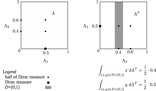
Figure 2.1. An illustration of the concept of flatness order. Let $\Lambda_{1}$ be the Dirac measure on $0.5$. Let $\Lambda_{2}$ be a half of the sum of the Dirac measures on $0.4$ and on $0.6$. The left-hand side shows a measure $\Lambda$ which witnesses that $\Lambda_{1}$ is at least as flat as $\Lambda_{2}$. The right-hand side gives an example of a set $D$ which proves that the transposed measure $\Lambda^{T}$ fails to witness that $\Lambda_{2}$ is at least as flat as $\Lambda_{1}$ (and indeed no such witness exists).

An illustration of the concept of flatness order is given in Figure 2.1. We can now state the main result of Section 4.4 of [12].

Proposition 2.22.

Suppose that we have two graphons $U\preceq W$. Then the measure $\boldsymbol{\Phi}_{U}$ is at least as flat as the measure $\boldsymbol{\Phi}_{W}$. Similarly, the measure $\boldsymbol{\Upsilon}_{U}$ is at least as flat as the measure $\boldsymbol{\Upsilon}_{W}$. Lastly, if $U\prec W$ then $\boldsymbol{\Phi}_{U}$ is strictly flatter than $\boldsymbol{\Phi}_{W}$.

2.7. Approximating a graphon by versions of a more structured graphon

In this section we state and prove Lemma 2.24, which is the key technical step for one of our main results, Theorem 3.28. Since the proof of Lemma 2.24 is quite complex, we first state a simplified version in Lemma 2.23. We use this simplification to explain some key features of the proof and motivate some further notation.

Lemma 2.23 (Simplified version of Proposition 2.31).

Suppose that $U,V\in\mathcal{W}_{0}$ and that $\mathcal{R}$ is a finite partition of $\Omega$ such that $V=U^{\Join\mathcal{R}}$. Then for each $\varepsilon>0$ we can find a number $N$ and measure preserving bijections $\left(\phi_{i}:\Omega\rightarrow\Omega\right)_{i=1}^{N}$ such that $\left\|V-\frac{\sum_{i=1}^{N}U^{\phi_{i}}}{N}\right\|_{1}<\varepsilon$.

While there are several possible proofs, the one which we need (and which we extend to prove Lemma 2.24) uses the probabilistic method. Let us sketch it now. Let $\mathcal{R}=\left\{\Omega_{1},\Omega_{2},\ldots,\Omega_{k}\right\}$. Suppose that we are given $\varepsilon$. We now take a large number $s$, and $N\gg s$. We partition each set $\Omega_{j}$ into sets $\llbracket\Omega_{j}\rrbracket_{1}^{s}\sqcup\llbracket\Omega_{j}\rrbracket_{2}^{s}\sqcup\ldots\sqcup\llbracket\Omega_{j}\rrbracket_{s}^{s}$ of the same measure (Definition 2.26 below introduces this formally). For each $j\in[k]$, we can randomly shuffle the sets $\left\{\llbracket\Omega_{j}\rrbracket_{1}^{s},\llbracket\Omega_{j}\rrbracket_{2}^{s},\ldots,\llbracket\Omega_{j}\rrbracket_{s}^{s}\right\}$. Putting these shuffles together, we obtain a random measure preserving bijection $\phi:\Omega\rightarrow\Omega$ with the property that

(2.15) $$\Omega_{j}=\phi\left(\Omega_{j}\right)\text{ for each $j\in[k]$,}$$

and hence a random version $U^{\phi}$ of $U$ (Definition 2.27 below introduces this formally). Such a random version typically blurs whatever structure there was in each rectangle $\Omega_{j}\times\Omega_{\ell}$ ($j,\ell\in[k]$). Hence, a rather straightforward application of the Law of Large Numbers gives that with high probability, the mean of independent random versions $U^{\phi_{1}},U^{\phi_{2}}\ldots,U^{\phi_{N}}$ approximates $V$ in the $L^{1}$-distance.

Our actual Lemma 2.24 strengthens Lemma 2.23 in two ways. Firstly, it assumes that $V\preceq U$ which is more general than $V=U^{\Join\mathcal{R}}$ for some finite partition $\mathcal{R}$. This represents only a minor complication in the proof as these properties are almost the same (see for example Lemma 2.28). So, we describe the second (and main) strengthening under the notationally more convenient assumption that $V=U^{\Join\mathcal{R}}$ for $\mathcal{R}=\left\{\Omega_{1},\Omega_{2},\ldots,\Omega_{k}\right\}$. In addition to the approximation property as in Lemma 2.23, we require that many of the pairs $U^{\phi_{2i-1}}$ and $U^{\phi_{2i}}$ are at least as far apart in the cut norm distance, as a constant multiple of $\delta_{\square}\left(U,V\right)$. (Note that this statement is void when $\delta_{\square}\left(U,V\right)=0$. Indeed in that case there is no way we could hope for such a property.) Let us explain why we expect this to occur for two independent random versions $U^{\phi_{2i-1}}$ and $U^{\phi_{2i}}$ with high probability. To this end, let us fix $S,T\subset\Omega$ for which we have $\left|\int_{S\times T}(U-V)\right|>\frac{\delta_{\square}\left(U,V\right)}{2}$. Without loss of generality, let us assume that $\int_{S\times T}(U-V)>\frac{\delta_{\square}\left(U,V\right)}{2}$. Let us now look at $U^{\phi_{2i-1}}$. We clearly have $\int_{S\times T}U=\int_{\phi_{2i-1}^{-1}(S)\times\phi_{2i-1}^{-1}(T)}U^{\phi_{2i-1}}$. Since $V$ is a step-function on $\mathcal{R}\times\mathcal{R}$, for any measure preserving bijection $\phi$ satisfying (2.15) we have $\int_{S\times T}V=\int_{\phi^{-1}\left(S\right)\times\phi^{-1}\left(T\right)}V$, and hence

(2.16) $$\int_{\phi_{2i-1}^{-1}(S)\times\phi_{2i-1}^{-1}(T)}(U^{\phi_{2i-1}}-V)>\frac{\delta_{\square}\left(U,V\right)}{2}\;.$$

Let us now look at $\int_{\phi_{2i-1}^{-1}(S)\times\phi_{2i-1}^{-1}(T)}U^{\phi_{2i}}$. As we said earlier (recall Footnote [g]), the version $U^{\phi_{2i}}$ with high probability blurs any structure on each rectangle $\Omega_{j}\times\Omega_{\ell}$. Thus, with high probability, $\int_{\phi_{2i-1}^{-1}(S)\times\phi_{2i-1}^{-1}(T)}U^{\phi_{2i}}\approx\int_{\phi_{2i-1}^{-1}(S)\times\phi_{2i-1}^{-1}(T)}V$. Combined with (2.16), this proves that $U^{\phi_{2i-1}}$ and $U^{\phi_{2i}}$ are far apart in the cut norm distance. In the actual proof, we need to deal with several technical difficulties.

Lemma 2.24.

Suppose that $U,V\in\mathcal{W}_{0}$ and $V\prec U$. Then for any $\varepsilon>0$ we can find an even number $N$ and measure preserving bijections $\left(\phi_{i}:\Omega\rightarrow\Omega\right)_{i=1}^{N}$ such that

(2.17) $$\left\|V-\frac{\sum_{i=1}^{N}U^{\phi_{i}}}{N}\right\|_{1}<\varepsilon\;.$$

Moreover, for at least half of the indices $i\in\left\{1,2,\ldots,\frac{N}{2}\right\}$ we have

(2.18) $$\left\|U^{\phi_{2i-1}}-U^{\phi_{2i}}\right\|_{\square}>\frac{\delta_{\square}\left(U,V\right)}{32}\;.$$

Remark 2.25.

Obviously, by rescaling, Lemma 2.24 can be extended to $U,V\in\mathcal{W}^{+}$.

The rest of this section is devoted to proving Lemma 2.24. The key construction in the proof of Lemma 2.24 is very similar to the proof of Lemma 9 in [13] (however, our proof is substantially more complex due to the additional property (2.18)). We borrow the following two definitions from [13].

Definition 2.26.

Given a set $A\subset[0,1]$ of positive measure and a number $s\in\mathbb{N}$, we can consider a partition $A=\llbracket A\rrbracket_{1}^{s}\sqcup\llbracket A\rrbracket_{2}^{s}\sqcup\ldots\sqcup\llbracket A\rrbracket_{s}^{s}$, where each set $\llbracket A\rrbracket_{i}^{s}$ has measure $\frac{\lambda(A)}{s}$ and for each $1\leq i<j\leq s$, the set $\llbracket A\rrbracket_{i}^{s}$ is entirely to the left of $\llbracket A\rrbracket_{j}^{s}$. These conditions define the partition $A=\llbracket A\rrbracket_{1}^{s}\sqcup\llbracket A\rrbracket_{2}^{s}\sqcup\ldots\sqcup\llbracket A\rrbracket_{s}^{s}$ uniquely, up to null sets. For each $i,j\in[s]$ there is a natural, uniquely defined (up to null sets), measure preserving almost-bijection $\chi_{i,j}^{A,s}:\llbracket A\rrbracket_{i}^{s}\rightarrow\llbracket A\rrbracket_{j}^{s}$ which preserves the order on the real line.

We can now give a definition of the model of random versions of a given graphon which we need. An illustration is given in Figure 2.2.

Figure 2.2. An illustration to Definitions 2.26 and 2.27. A sample partition $\mathcal{R}=\left\{\Omega_{1},\Omega_{2}\right\}$ of $[0,1]$ in the top left figure. To create $\mathbb{W}(\Gamma,\mathcal{R},s=3)$, the unit interval is partitioned as in the top right figure. Finally, for randomly chosen permutations $\pi_{1},\pi_{2}$, the unit interval is effectively reshuffled as in the bottom figure.

Definition 2.27.

Suppose that $\Gamma:[0,1]^{2}\rightarrow[0,1]$ is a graphon. For a finite partition $\mathcal{R}=\left\{\Omega_{1},\Omega_{2},\ldots,\Omega_{k}\right\}$ of $[0,1]$ and for $s\in\mathbb{N}$, we define a discrete probability distribution $\mathbb{W}(\Gamma,\mathcal{R},s)$ on versions of $\Gamma$ as follows. We take $\pi_{1},\ldots,\pi_{k}:[s]\rightarrow[s]$ independent uniformly random permutations. After these are fixed, we define a sample $W\sim\mathbb{W}(\Gamma,\mathcal{R},s)$ by

$$W(x,y)=\Gamma\left(\chi_{p,\pi_{i}(p)}^{\Omega_{i},s}(x),\chi_{q,\pi_{j}(q)}^{\Omega_{j},s}(y)\right)\quad\mbox{when $x\in\llbracket\Omega_{i}\rrbracket_{p}^{s}$, $y\in\llbracket\Omega_{j}\rrbracket_{q}^{s}$, $i,j\in[k]$, $p,q\in[s]$}\;.$$

This defines the sample $W:[0,1]^{2}\rightarrow[0,1]$ uniquely up to null sets, and thus defines the whole distribution $\mathbb{W}(\Gamma,\mathcal{R},s)$. Observe that $\mathbb{W}(\Gamma,\mathcal{R},s)$ is supported on (some) versions of $\Gamma$. We call the sets $\llbracket\Omega_{j}\rrbracket_{q}^{s}$ stripes.

We shall also need the following technical lemmas.

Lemma 2.28.

Let $V\preceq U$ be two graphons on $\Omega^{2}$ and $\varepsilon>0$. Then there is a measure preserving bijection $\varphi:\Omega\rightarrow\Omega$ and a finite partition $\mathcal{R}$ of $\Omega$ such that

$$\left\|V-\left(U^{\varphi}\right)^{\Join\mathcal{R}}\right\|_{1}<\varepsilon.$$

Proof.

Use Lemma 2.8 to find a finite partition $\mathcal{R}$ such that $\left\|V-V^{\Join\mathcal{R}}\right\|_{1}<\frac{\varepsilon}{2}$. By the definition of $V\preceq U$ we may find a sequence $\left\{U^{\varphi_{i}}\right\}_{i\in\mathbb{N}}$ of versions of $U$ such that $U^{\varphi_{i}}\overset{\mathrm{w}^{*}}{\;\longrightarrow\;}V$. By Lemma 2.9, we have $\left(U^{\varphi_{i}}\right)^{\Join\mathcal{R}}\overset{\mathrm{w}^{*}}{\;\longrightarrow\;}V^{\Join\mathcal{R}}$. Since on the left-hand side, we have step-functions on the same grid $\mathcal{R}\times\mathcal{R}$, the weak* convergence is in this case equivalent to the convergence in $\left\|\cdot\right\|_{1}$, $\left(U^{\varphi_{i}}\right)^{\Join\mathcal{R}}\overset{\|\cdot\|_{1}}{\;\longrightarrow\;}V^{\Join\mathcal{R}}$. Now, we can find $i\in\mathbb{N}$ such that $\left\|V-\left(U^{\varphi_{i}}\right)^{\Join\mathcal{R}}\right\|_{1}\leq\left\|V-V^{\Join\mathcal{R}}\right\|_{1}+\left\|V^{\Join\mathcal{R}}-\left(U^{\varphi_{i}}\right)^{\Join\mathcal{R}}\right\|_{1}<\varepsilon$. ∎

Lemma 2.29.

Let $A\subset\left[0,1\right]$ be a measurable set, $\mathcal{R}=\left\{\Omega_{1},\dots,\Omega_{k}\right\}$ be a finite partition of $\left[0,1\right]$ and $\varepsilon>0$. Then there is $s_{0}\in\mathbb{N}$ such that for every $s\geq s_{0}$ we may find a collection $\mathcal{I_{A}}\subset\left[k\right]\times\left[s\right]$ such that for the symmetric difference of $A$ and $\bigcup_{\left(i,x\right)\in\mathcal{I}_{A}}\left\llbracket\Omega_{i}\right\rrbracket_{x}^{s}$ we have

$$\nu\left(A\diamond\bigcup_{\left(i,x\right)\in\mathcal{I}_{A}}\left\llbracket\Omega_{i}\right\rrbracket_{x}^{s}\right)<\varepsilon.$$

Proof.

First we demonstrate that it is enough to show the lemma for the special case when $\mathcal{R}$ is an interval partition. Suppose that $A\subset\left[0,1\right]$ and $\varepsilon>0$ is given. We may find a measurable almost-bijection $\varphi$ such that the restriction of $\varphi$ to each $\Omega_{j}$ preserves the order of the real line and such that $\varphi\left(\mathcal{R}\right)$ is an interval partition. Then we find the correct $s_{0}\in\mathbb{N}$ when applied for $\varphi\left(A\right)$. It is clear that this $s_{0}\in\mathbb{N}$ works because $\varphi\left(\left\llbracket\Omega_{i}\right\rrbracket_{x}^{s}\right)=\left\llbracket\varphi\left(\Omega_{i}\right)\right\rrbracket_{x}^{s}$.

If $\mathcal{R}$ is a finite interval partition then we can work in each interval separately. This implies that we may restrict ourselves to the case where $\mathcal{R}=\left\{\left[0,1\right]\right\}$. The latter is a basic fact about the Lebesgue measure. ∎

Lemma 2.30.

Let $U\in\mathcal{W}_{0}$, $\mathcal{R}=\left\{\Omega_{1},\dots,\Omega_{k}\right\}$ be a finite partition and $\varepsilon>0$. Then there is $s_{0}\in\mathbb{N}$ such that for every $s\geq s_{0}$ we have $\left\|U-U^{\Join\left\llbracket\mathcal{R}\right\rrbracket^{s}}\right\|_{1}<\varepsilon$ where

$$\left\llbracket\mathcal{R}\right\rrbracket^{s}=\left\{\left\llbracket\Omega_{i}\right\rrbracket_{x}^{s}:\left(i,x\right)\in\left[k\right]\times\left[s\right]\right\}.$$

Proof.

Using Lemma 2.29, it is straightforward to show that the assertion is true if there is a finite partition $\mathcal{P}=\{P_{1},\ldots,P_{\ell}\}$ of $\Omega$ such that $U$ is constant on each $P_{i}\times P_{j}$. To prove the general case, use Lemma 2.8 to find a suitable partition $\mathcal{P}$ of $\Omega$, then apply the previous observation to $U^{\Join\mathcal{P}}$ and use the inequality

$$\|U-U{}^{\Join\left\llbracket\mathcal{R}\right\rrbracket^{s}}\|_{1}\leq\|U-U^{\Join\mathcal{P}}\|_{1}+\|U^{\Join\mathcal{P}}-(U^{\Join\mathcal{P}})^{\Join\left\llbracket\mathcal{R}\right\rrbracket^{s}}\|_{1}+\|(U^{\Join\mathcal{P}})^{\Join\left\llbracket\mathcal{R}\right\rrbracket^{s}}-U{}^{\Join\left\llbracket\mathcal{R}\right\rrbracket^{s}}\|_{1}\>.$$

∎

Proposition 2.31.

Let $U$ be a graphon, $\mathcal{R}=\left\{\Omega_{1},\dots,\Omega_{k}\right\}$ a finite partition of $\left[0,1\right]$ and $\varepsilon>0$. Then there is $s_{0}\in\mathbb{N}$ such that for every $s\geq s_{0}$ there is $N_{0}\in\mathbb{N}$ such that for every $N\geq N_{0}$, an independently chosen random $N$-tuple $\left(W_{i}\sim\mathbb{W}\left(U,\mathcal{R},s\right)\right)_{i=1}^{N}$ satisfies

(2.19) $$\left\|U^{\Join\mathcal{R}}-\frac{\sum_{i=1}^{N}W_{i}}{N}\right\|_{1}<\varepsilon$$

with probability at least $0.9$.

Proof.

We will set $s_{0},s,N_{0},N$ later, and start with some bounds that hold for all $s$ and $N$, which we from now on suppose to be fixed. The idea is to split (2.19) to the contributions of individual parts $\left(\llbracket\Omega_{i}\rrbracket_{x}^{s}\times\llbracket\Omega_{j}\rrbracket_{y}^{s}\right)_{i,j\in[k],x,y\in[s]}$.

We call a quadruple $(i,j,x,y)\in[k]\times[k]\times[s]\times[s]$ a diagonal quadruple if $i=j$ and $x=y$. A quadruple $(i,j,p,q)\in[k]\times[k]\times[s]\times[s]$ is off-diagonal of Type I if $i\neq j$, and it is off-diagonal of Type II if $i=j$ and $x\neq y$.

Claim (Claim A).

Suppose that $(i,j,x,y)\in[k]\times[k]\times[s]\times[s]$ is an off-diagonal quadruple. Then for each $a>0$ we have with probability at least $1-2\exp\left(-\frac{a^{2}N}{2}\right)$ that

$$\left|\frac{1}{s^{2}}\int_{\Omega_{i}\times\Omega_{j}}U\mathrm{d}\nu^{\otimes 2}-\frac{1}{N}\sum_{\ell=1}^{N}\int_{\llbracket\Omega_{i}\rrbracket_{x}^{s}\times\llbracket\Omega_{j}\rrbracket_{y}^{s}}W_{\ell}\mathrm{d}\nu^{\otimes 2}\right|\leq a+\frac{2\nu^{\otimes 2}(\Omega_{i}\times\Omega_{j})}{s^{2}\left(s-1\right)}\;.$$

Proof of Claim A.

For each $\ell\in[N]$, we define

$$Y_{\ell}:=\int_{\llbracket\Omega_{i}\rrbracket_{x}^{s}\times\llbracket\Omega_{j}\rrbracket_{y}^{s}}W_{\ell}\mathrm{d}\nu^{\otimes 2}\;.$$

Then $Y_{\ell}:\mathbb{W}\left(U,\mathcal{R},s\right)\to\left[0,1\right]$ is a random variable with the expectation

$$e_{1}:=\frac{1}{s^{2}}\cdot\int_{\Omega_{i}\times\Omega_{j}}U\mathrm{d}\nu^{\otimes 2}$$

if $(i,j,x,y)$ if off-diagonal of Type I, or

$$e_{2}:=\frac{1}{s\left(s-1\right)}\int_{\Omega_{i}\times\Omega_{j}\setminus\cup_{d=1}^{s}\llbracket\Omega_{i}\rrbracket_{d}^{s}\times\llbracket\Omega_{j}\rrbracket_{d}^{s}}U\mathrm{d}\nu^{\otimes 2}=\left(\frac{1}{s^{2}}\int_{\Omega_{i}\times\Omega_{j}}U\mathrm{d}\nu^{\otimes 2}\right)\pm\frac{2\nu^{\otimes 2}\left(\Omega_{i}\times\Omega_{j}\right)}{s^{2}\left(s-1\right)}$$

if $(i,j,x,y)$ if off-diagonal of Type II. To see this, consider first the case of Type I. In that case, using the notation from Definition 2.27, we have a random permutation $\pi_{i}$ permuting stripes of $\Omega_{i}$ and a different random permutation $\pi_{j}$ permuting stripes of $\Omega_{j}$. Such a pair of random permutations induces a permutation of the grid on $\Omega_{i}\times\Omega_{j}$ such that the probability that any given cell is placed onto the cell $\llbracket\Omega_{i}\rrbracket_{x}^{s}\times\llbracket\Omega_{j}\rrbracket_{y}^{s}$ is $\frac{1}{s^{2}}$, which justifies that the average is $e_{1}$ in this case. Similarly, in the case of Type II (i.e., $i=j$), we have one permutation $\pi_{i}$ which permutes simultaneously rows and columns of the grid on $\Omega_{i}\times\Omega_{i}$. In that case, the probability that any given off-diagonal cell is placed onto the cell $\llbracket\Omega_{i}\rrbracket_{x}^{s}\times\llbracket\Omega_{i}\rrbracket_{y}^{s}$ is $\frac{1}{s(s-1)}$.

Observe that $\left(Y_{\ell}\right)_{\ell=1}^{N}$ are independent random variables. Thus, the Chernoff bound (Lemma 2.2) gives us that for each $a>0$ we have with probability at least $1-2\exp\left(-\frac{a^{2}N^{2}}{2N}\right)=1-2\exp\left(-\frac{a^{2}N}{2}\right)$ that

(2.20) $$\left|\frac{1}{s^{2}}\int_{\Omega_{i}\times\Omega_{j}}U\mathrm{d}\nu^{\otimes 2}-\frac{1}{N}\sum_{\ell=1}^{N}\int_{\llbracket\Omega_{i}\rrbracket_{x}^{s}\times\llbracket\Omega_{j}\rrbracket_{y}^{s}}W_{\ell}\mathrm{d}\nu^{\otimes 2}\right|=\left|e_{1}-\left(\frac{1}{N}\sum_{\ell=1}^{N}Y_{\ell}\right)\right|\leq a$$

in the case of off-diagonal quadruple of Type I and

(2.21) $$\left|\frac{1}{s^{2}}\int_{\Omega_{i}\times\Omega_{j}}U\mathrm{d}\nu^{\otimes 2}-\frac{1}{N}\sum_{\ell=1}^{N}\int_{\llbracket\Omega_{i}\rrbracket_{x}^{s}\times\llbracket\Omega_{j}\rrbracket_{y}^{s}}W_{\ell}\mathrm{d}\nu^{\otimes 2}\right| \leq$$

$$\leq\left|e_{2}-\left(\frac{1}{N}\sum_{\ell=1}^{N}Y_{\ell}\right)\right|+\frac{2\nu^{\otimes 2}\left(\Omega_{i}\times\Omega_{j}\right)}{s^{2}\left(s-1\right)} \leq a+\frac{2\nu^{\otimes 2}\left(\Omega_{i}\times\Omega_{j}\right)}{s^{2}\left(s-1\right)}$$

in the case of off-diagonal quadruple of Type II. Hence, (2.20) and (2.21) give the statement of the claim. ∎

Take $s_{0}\geq 3$ that satisfies Lemma 2.30 with $\frac{\varepsilon}{2}$, and such that $\frac{k^{2}+3}{s_{0}-1}<\frac{\varepsilon}{2}$. Then for every $s\geq s_{0}$ we may find $N_{0}$ such that for every $N\geq N_{0}$ we have $1-2\exp\left(-\frac{\left(\frac{1}{s^{3}}\right)^{2}N}{2}\right)>1-\frac{1}{10k^{2}s^{2}}$. We have

$$\left\|U^{\Join\mathcal{R}}-\frac{1}{N}\sum_{\ell=1}^{N}W_{\ell}\right\|_{1} \leq\left\|U^{\Join\mathcal{R}}-\frac{1}{N}\sum_{\ell=1}^{N}\left(W_{\ell}\right)^{\Join\left\llbracket\mathcal{R}\right\rrbracket^{s}}\right\|_{1}+\left\|\frac{1}{N}\sum_{\ell=1}^{N}\left(W_{\ell}\right)^{\Join\left\llbracket\mathcal{R}\right\rrbracket^{s}}-\frac{1}{N}\sum_{\ell=1}^{N}W_{\ell}\right\|_{1}$$

$$\leq\left\|U^{\Join\mathcal{R}}-\frac{1}{N}\sum_{\ell=1}^{N}\left(W_{\ell}\right)^{\Join\left\llbracket\mathcal{R}\right\rrbracket^{s}}\right\|_{1}+\frac{\varepsilon}{2}.$$

The following simple observation allows us to use Claim A:

$$\left\|U^{\Join\mathcal{R}}-\frac{1}{N}\sum_{\ell=1}^{N}\left(W_{\ell}\right)^{\Join\left\llbracket\mathcal{R}\right\rrbracket^{s}}\right\|_{1}$$

$$= \sum_{\left(i,j,x,y\right)\in\left[k\right]\times\left[k\right]\times\left[s\right]\times\left[s\right]}\int_{\llbracket\Omega_{i}\rrbracket_{x}^{s}\times\llbracket\Omega_{j}\rrbracket_{y}^{s}}$$

$$\,\,\,\,\,\left|\frac{1}{\nu^{\otimes 2}(\Omega_{i}\times\Omega_{j})}\int_{\Omega_{i}\times\Omega_{j}}U\mathrm{d}\nu^{\otimes 2}-\frac{1}{N}\sum_{\ell=1}^{N}\frac{s^{2}}{\nu^{\otimes 2}(\Omega_{i}\times\Omega_{j})}\int_{\llbracket\Omega_{i}\rrbracket_{x}^{s}\times\llbracket\Omega_{j}\rrbracket_{y}^{s}}W_{\ell}\mathrm{d}\nu^{\otimes 2}\right|\mathrm{d}\nu^{\otimes 2}$$

$$= \sum_{\left(i,j,x,y\right)\in\left[k\right]\times\left[k\right]\times\left[s\right]\times\left[s\right]}\left|\frac{1}{s^{2}}\int_{\Omega_{i}\times\Omega_{j}}U\mathrm{d}\nu^{\otimes 2}-\frac{1}{N}\sum_{\ell=1}^{N}\int_{\llbracket\Omega_{i}\rrbracket_{x}^{s}\times\llbracket\Omega_{j}\rrbracket_{y}^{s}}W_{\ell}\mathrm{d}\nu^{\otimes 2}\right|\;.$$

Claim A applied with $a=\frac{1}{s^{3}}$ gives that with probability at least $1-\left(\sum_{i,j\in\left[k\right]}\sum_{x,y\in[s]}\frac{1}{10k^{2}s^{2}}\right)=0.9$ we have

$$\sum_{\left(i,j,x,y\right)\in\left[k\right]\times\left[k\right]\times\left[s\right]\times\left[s\right]}\left|\frac{1}{s^{2}}\int_{\Omega_{i}\times\Omega_{j}}U\mathrm{d}\nu^{\otimes 2}-\frac{1}{N}\sum_{\ell=1}^{N}\int_{\llbracket\Omega_{i}\rrbracket_{x}^{s}\times\llbracket\Omega_{j}\rrbracket_{y}^{s}}W_{\ell}\mathrm{d}\nu^{\otimes 2}\right|$$

$$\leq \sum_{i,j\in\left[k\right]\times\left[k\right]}s^{2}\left(a+\frac{2\nu^{\otimes 2}\left(\Omega_{i}\times\Omega_{j}\right)}{s^{2}\left(s-1\right)}\right)+\sum_{(i,x)\in\left[k\right]\times\left[s\right]}\nu^{\otimes 2}\left(\llbracket\Omega_{i}\rrbracket_{x}^{s}\times\llbracket\Omega_{i}\rrbracket_{x}^{s}\right)$$

$$\leq k^{2}s^{2}a+\frac{2}{s-1}+\frac{1}{s}\leq\frac{k^{2}+3}{s-1}<\frac{\varepsilon}{2}\;.$$

∎

Proposition 2.32.

Let $U$ be a graphon, $\mathcal{R}=\left\{\Omega_{1},\dots,\Omega_{k}\right\}$ be a finite partition of $\left[0,1\right]$. Then there is $s_{0}\in\mathbb{N}$ such that for every $s\geq s_{0}$, a random graphon $W\sim\mathbb{W}\left(U,\mathcal{R},s\right)$ satisfies

$$\left\|U-W\right\|_{\square}>\frac{\delta_{\square}\left(U,U^{\Join\mathcal{R}}\right)}{8}-\frac{2}{s^{\frac{1}{4}}}$$

with probability at least $1-\exp\left(-\frac{\sqrt{s}}{8k}\right)$.

Proof.

Put $V=U^{\Join\mathcal{R}}$ and write $\delta=\delta_{\square}\left(U,V\right)$. By Lemma 2.5 we may find $S_{0},T_{0}\subset\Omega$ such that $S_{0}\cap T_{0}=\emptyset$ and

$$\left|\int_{S_{0}\times T_{0}}(U-V)\right|\geq\frac{\delta}{4}\;.$$

By a slight modification of Lemma 2.29 there is $s_{0}\geq 3$ such that for every $s\geq s_{0}$ there are $S,T\subset\Omega$ that are unions of stripes such that

$$\left|\int_{S\times T}(U-V)\right|\geq\frac{\delta}{8}$$

and $S\cap T=\emptyset$. Now fix $s\geq s_{0}$ and denote $\mathcal{I}_{S},\mathcal{I}_{T}\subset\left[k\right]\times\left[s\right]$ the sets of indices giving the corresponding stripes, i.e.,

$$S=\bigcup_{\left(i,x\right)\in\mathcal{I}_{S}}\left\llbracket\Omega_{i}\right\rrbracket_{x}^{s}$$

and similarly for $T$. Define $\mathcal{I}_{S}^{i}=\left\{x\in\left[s\right]:\left(i,x\right)\in\mathcal{I}_{S}\right\}$, $\mathcal{C}_{S}=\left\{\left\llbracket\Omega_{i}\right\rrbracket_{x}^{s}\right\}_{\left(i,x\right)\in\mathcal{I}_{S}}$ and $\mathcal{C}_{S}^{i}=\left\{\left\llbracket\Omega_{i}\right\rrbracket_{x}^{s}\right\}_{x\in\mathcal{I}_{S}^{i}}$, similarly define $\mathcal{I}_{T}^{i}$, $\mathcal{C}_{T}$ and $\mathcal{C}_{T}^{i}$.

We may assume that $S_{i}:=\bigcup\mathcal{C}_{S}^{i}$ is on the left side of $\Omega_{i}$ and that $T_{i}:=\bigcup\mathcal{C}_{T}^{i}$ is exactly next to it. To see this note that if $\mathcal{C}_{S}^{i}$ and $\mathcal{C}_{T}^{i}$ are in some general position, then we may find a measure preserving bijection $\varphi$ that is invariant on each $\Omega_{i}$ and permutes the stripes accordingly. Note that this is possible because $S,T$ are disjoint. Then for $\mathcal{C}_{S}^{i},\mathcal{C}_{T}^{i}$ in the general position use the same argument with conjugation by $\varphi$ as in Lemma 2.29.

Define the random variable $Z:\mathbb{W}\left(U,\mathcal{R},s\right)\to\mathbb{R}$ as

$$Z\left(W\right)=\int_{S\times T}W\mathrm{d}\nu^{\otimes 2}.$$

Claim (Claim B).

We have $\mathbf{E}\left[Z\right]=\int_{S\times T}V\mathrm{d}\nu^{\otimes 2}\pm\frac{1}{s-1}$.

Proof of Claim B.

For fixed $i,j\in[k]$ define $Z_{i,j}\left(W\right)=\int_{S_{i}\times T_{j}}W\mathrm{d}\nu^{\otimes 2}$. Then $Z=\sum_{i,j\in[k]}Z_{i,j}$ and also $\mathbf{E}\left[Z\right]=\sum_{i,j\in[k]}\mathbf{E}\left[Z_{i,j}\right]$. It suffices to show that $\mathbf{E}\left[Z_{i,j}\right]=\int_{S_{i}\times T_{j}}V\mathrm{d}\nu^{\otimes 2}$ if $i\not=j$ and $\mathbf{E}\left[Z_{i,i}\right]=\int_{S_{i}\times T_{i}}V\mathrm{d}\nu^{\otimes 2}\pm\frac{\nu^{\otimes 2}\left(\Omega_{i}\times\Omega_{i}\right)}{s-1}$ if $i=j$.

We use the notation from the proof of Proposition 2.31. Take an off-diagonal quadruple $\left(i,j,x,y\right)\in\left[k\right]\times\left[k\right]\times\left[s\right]\times\left[s\right]$ and define

$$Y_{i,j,x,y}=\int_{\llbracket\Omega_{i}\rrbracket_{x}^{s}\times\llbracket\Omega_{j}\rrbracket_{y}^{s}}W\mathrm{d}\nu^{\otimes 2}\ .$$

There are two cases depending on the type of $\left(i,j,x,y\right)$. Suppose that $\left(i,j,x,y\right)$ is of Type I. Then we have

$$\mathbf{E}\left[Y_{i,j,x,y}\right]=\frac{1}{s^{2}}\cdot\int_{\Omega_{i}\times\Omega_{j}}U\mathrm{d}\nu^{\otimes 2}=\frac{1}{s^{2}}\cdot\int_{\Omega_{i}\times\Omega_{j}}V\mathrm{d}\nu^{\otimes 2}\;,$$

and summing over all $\left(x,y\right)\in\mathcal{I}_{S}^{i}\times\mathcal{I}_{T}^{j}$ we get for $i\neq j$ that

$$\mathbf{E}\left[Z_{i,j}\right]=\frac{\left|\mathcal{I}_{S}^{i}\right|\times\left|\mathcal{I}_{T}^{j}\right|}{s^{2}}\int_{\Omega_{i}\times\Omega_{j}}V\mathrm{d}\nu^{\otimes 2}=\int_{S_{i}\times T_{j}}V\mathrm{d}\nu^{\otimes 2}.$$

Suppose that $\left(i,i,x,y\right)$ is of Type II. Then we have

$$\mathbf{E}\left[Y_{i,i,x,y}\right]=\left(\frac{1}{s^{2}}\int_{\Omega_{i}\times\Omega_{i}}V\mathrm{d}\nu^{\otimes 2}\right)\pm\frac{2\nu^{\otimes 2}\left(\Omega_{i}\times\Omega_{i}\right)}{s^{2}\left(s-1\right)}\;,$$

and summing over all $\left(x,y\right)\in\mathcal{I}_{S}^{i}\times\mathcal{I}_{T}^{i}$ (with $x$ and $y$ distinct) we get for every $i$ that

$$\mathbf{E}\left[Z_{i,i}\right] =\frac{\left|\mathcal{I}_{S}^{i}\right|\times\left|\mathcal{I}_{T}^{i}\right|}{s^{2}}\left(\int_{\Omega_{i}\times\Omega_{i}}V\mathrm{d}\nu^{\otimes 2}\pm\frac{2\nu^{\otimes 2}\left(\Omega_{i}\times\Omega_{i}\right)}{\left(s-1\right)}\right)$$

$$=\int_{S_{i}\times T_{i}}V\mathrm{d}\nu^{\otimes 2}\pm\frac{\nu^{\otimes 2}\left(\Omega_{i}\times\Omega_{i}\right)}{s-1}$$

because $\frac{\left|\mathcal{I}_{S}^{i}\right|\times\left|\mathcal{I}_{T}^{i}\right|}{s^{2}}\leq\frac{1}{2}$. ∎

In order to use the Method of Bounded Differences we introduce the following correspondence between permutations that induce $\mathbb{W}\left(U,\mathcal{R},s\right)$ and $\left[0,1\right]^{k\times s}$ (which we view as functions from $[k]\times[s]$ to $[0,1]$). Namely, for each $f\in[k]\times[s]\rightarrow[0,1]$ which is injective we define a permutation $\alpha_{f}$ of $[k]\times[s]$ such that $\alpha_{f}(\{i\}\times[s])=\{i\}\times[s]$ for each $i$, and such that the relative position of $\alpha_{f}(i,x)$ inside the block $\{i\}\times[s]$ is the same as the relative position of $f\left(i,x\right)$ inside the set of numbers $\left\{f\left(i,y\right)\right\}_{y\in\left[s\right]}$. We leave $\alpha_{f}$ undefined for non-injective functions, which form a nullset on $\left[0,1\right]^{k\times s}$. One can verify that the assignment $f\mapsto(\alpha_{f})^{-1}$, which maps each $f$ to the inverse of $\alpha_{f}$, is measure preserving where we have the Lebesgue measure on $\left[0,1\right]^{k\times s}$ and the uniform measure on the permutations of $\left[k\right]\times\left[s\right]$ that fix the first coordinate. Note that these are exactly the permutations that naturally induce $\mathbb{W}\left(U,\mathcal{R},s\right)$. Hence, we may consider the random variable $Z$ to be defined on $\left[0,1\right]^{k\times s}$ with values in $\mathbb{R}$.

We show that $Z$ satisfies the assumptions of Lemma 2.3(a). Recall that we assume that each $S_{i}$ is concentrated on the left-most part of the interval $\Omega_{i}$ and $T_{i}$ is exactly next to it. Suppose that $f,f^{\prime}\in\left[0,1\right]^{k\times s}$ differ in at most one coordinate in the $i$-th block. Then

$$\left|(\alpha_{f})^{-1}\left(\mathcal{I}_{S}^{i}\right)\diamond(\alpha_{f^{\prime}})^{-1}\left(\mathcal{I}_{S}^{i}\right)\right|\leq 2\quad\mbox{and}\quad\left|(\alpha_{f})^{-1}\left(\mathcal{I}_{T}^{i}\right)\diamond(\alpha_{f^{\prime}})^{-1}\left(\mathcal{I}_{T}^{i}\right)\right|\leq 2.$$

Then we may compute

$$\left|Z\left(f\right)-Z\left(f^{\prime}\right)\right| =\left|\int_{S\times T}U^{(\alpha_{f})^{-1}}\mathrm{d}\nu^{\otimes 2}-\int_{S\times T}U^{(\alpha_{f^{\prime}})^{-1}}\mathrm{d}\nu^{\otimes 2}\right|$$

$$=\left|\int_{(\alpha_{f})^{-1}\left(S\right)\times(\alpha_{f})^{-1}\left(T\right)}U\mathrm{d}\nu^{\otimes 2}-\int_{(\alpha_{f^{\prime}})^{-1}\left(S\right)\times(\alpha_{f^{\prime}})^{-1}\left(T\right)}U\mathrm{d}\nu^{\otimes 2}\right|$$

$$\leq\nu^{\otimes 2}\left(\left((\alpha_{f})^{-1}\left(S\right)\times(\alpha_{f})^{-1}\left(T\right)\right)\diamond\left((\alpha_{f^{\prime}})^{-1}\left(S\right)\times(\alpha_{f^{\prime}})^{-1}\left(T\right)\right)\right)$$

$$\leq 4\frac{\nu\left(\Omega_{i}\right)}{s}\leq\frac{4}{s}.$$

By Lemma 2.3(a) we have

$$\mathbf{P}\left[\left|Z-\mathbf{E}Z\right|>d\right]\leq\exp\left(-\frac{d^{2}s}{8k}\right)\;,\text{for any $d>0$.}$$

In particular, taking $d=s^{-\frac{1}{4}}$ we have

$$\mathbf{P}\left[\left|Z-\mathbf{E}Z\right|>s^{-\frac{1}{4}}\right]\leq\exp\left(-\frac{\sqrt{s}}{8k}\right)$$

and therefore with probability at least $1-\exp\left(-\frac{\sqrt{s}}{8k}\right)$ we have that

(2.22) $$\left|Z\left(W\right)-\mathbf{E}Z\right|\leq s^{-\frac{1}{4}}$$

for $W\in\mathbb{W}\left(U,\mathcal{R},s\right)$. We conclude that with probability at least $1-\exp\left(-\frac{\sqrt{s}}{8k}\right)$ we have that

$$\left\|W-U\right\|_{\square} \geq\left|\int_{S\times T}U\mathrm{d}\nu^{\otimes 2}-\int_{S\times T}W\mathrm{d}\nu^{\otimes 2}\right|$$

$$\geq\left|\int_{S\times T}U\mathrm{d}\nu^{\otimes 2}-\int_{S\times T}V\mathrm{d}\nu^{\otimes 2}\right|-\left|\int_{S\times T}V\mathrm{d}\nu^{\otimes 2}-\int_{S\times T}W\mathrm{d}\nu^{\otimes 2}\right|$$

$$\geq\frac{\delta}{8}-\left|Z\left(W\right)-\left(\mathbf{E}\left[Z\right]\pm\frac{1}{s-1}\right)\right|$$

by (2.22) $$\geq\frac{\delta}{8}-\frac{1}{s-1}-\frac{1}{s^{\frac{1}{4}}}>\frac{\delta}{8}-\frac{2}{s^{\frac{1}{4}}}\;,$$

as was needed (we used that $s\geq s_{0}\geq 3$ in the last inequality). ∎

Now we are ready to prove Lemma 2.24.

Proof of Lemma 2.24.

Let $\delta:=\delta_{\square}\left(V,U\right)$. By Fact 2.18, we have that $\delta>0$. First use Lemma 2.28 to approximate $V$ by some $\left(U^{\varphi}\right)^{\Join\mathcal{R}}$ such that $\left\|V-\left(U^{\varphi}\right)^{\Join\mathcal{R}}\right\|_{1}<\min\left(\frac{\varepsilon}{2},\frac{\delta}{2}\right)$. We may assume without loss of generality that $\varphi$ is the identity and therefore work with $U^{\Join\mathcal{R}}$ instead of $\left(U^{\varphi}\right)^{\Join\mathcal{R}}$. We have

$$\delta_{\square}\left(U,U^{\Join\mathcal{R}}\right)\geq\delta_{\square}\left(V,U\right)-\delta_{\square}\left(V,U^{\Join\mathcal{R}}\right)\geq\delta_{\square}\left(V,U\right)-\left\|V-U^{\Join\mathcal{R}}\right\|_{1}>\frac{\delta}{2}\;.$$

We use Proposition 2.31 and Proposition 2.32 to find $s\in\mathbb{N}$ and an even number $N$ such that $\left\|U-W\right\|_{\square}>\frac{\delta}{32}$ for $W\in\mathbb{W}\left(U,\mathcal{R},s\right)$ with probability at least $0.9$, and also $\left\|U^{\Join\mathcal{R}}-\frac{\sum_{k=1}^{N}W_{k}}{N}\right\|_{1}<\frac{\varepsilon}{2}$ for $\left(W_{k}\right)_{k=1}^{N}\in\left(\mathbb{W}\left(U,\mathcal{R},s\right)\right)^{N}$ with probability at least $0.9$.

Define a random variable $Q:\left(\mathbb{W}\left(U,\mathcal{R},s\right)\right)^{N}\rightarrow\mathbb{R}$,

$$Q:\left(W_{k}\right)_{k=1}^{N}\mapsto\frac{2}{N}\cdot\left|\left\{k\in[N/2]:\left\|W_{2k-1}-W_{2k}\right\|_{\square}\leq\frac{\delta}{32}\right\}\right|.$$

Note that for any $U^{*}\in\mathbb{W}(U,\mathcal{R},s)$ , the distributions $\mathbb{W}(U,\mathcal{R},s)$ and $\mathbb{W}(U^{*},\mathcal{R},s)$ on versions of $U$ coincide with probability $1$. So for every $k\in[N/2]$, we can equivalently first sample $W_{2k-1}\sim\mathbb{W}(U,\mathcal{R},s)$, and then sample $W_{2k}\sim\mathbb{W}(W_{2k-1},\mathcal{R},s)$. Thus, for a fixed $k\in[N/2]$ the probability that $\left\|W_{2k-1}-W_{2k}\right\|_{\square}>\frac{\delta}{32}$ is at least $0.9$ due to Proposition 2.32. Hence, $\mathbf{E}\left[Q\right]\leq 0.1$. By Markov’s inequality, $\mathbf{P}\left[Q\geq 0.4\right]\leq 0.25$. By the union bound, with probability at most $0.35$ we have that $Q\geq 0.4$ or that $\left\|U^{\Join\mathcal{R}}-\frac{\sum_{k=1}^{N}W_{k}}{N}\right\|_{1}\geq\frac{\varepsilon}{2}$. In particular, there exists a choice $\left(U^{\phi_{k}}\right)_{k=1}^{N}=\left(W_{k}\right)_{k=1}^{N}$ of an $N$-tuple of versions of $U$ which does not have any of these two <<bad>> properties. Such an $N$-tuple $\left(U^{\phi_{k}}\right)_{k=1}^{N}$ satisfies (2.18) since $Q<0.4<0.5$. It also satisfies (2.17) since

$$\left\|V-\frac{\sum_{i=1}^{N}U^{\phi_{i}}}{N}\right\|_{1}\leq\left\|V-U^{\Join\mathcal{R}}\right\|_{1}+\left\|U^{\Join\mathcal{R}}-\frac{\sum_{i=1}^{N}U^{\phi_{i}}}{N}\right\|_{1}<\frac{\varepsilon}{2}+\frac{\varepsilon}{2}=\varepsilon\;.$$

∎

3. Cut distance identifying graphon parameters

3.1. Basics

In [12], we based our treatment of the cut distance on $\mathbf{ACC}_{\mathrm{w}*}\left(W_{1},W_{2},W_{3},\ldots\right)$ and $\mathbf{\mathbf{LIM}_{\mathrm{w}*}}\left(W_{1},W_{2},W_{3},\ldots\right)$, which are sets of functions. In contrast, the key objects in [13] are the sets of numerical values

$$\left\{\mathrm{INT}_{f}(W):W\in\mathbf{ACC}_{\mathrm{w}*}\left(W_{1},W_{2},W_{3},\ldots\right)\right\}\text{ and }\left\{\mathrm{INT}_{f}(W):W\in\mathbf{\mathbf{LIM}_{\mathrm{w}*}}\left(W_{1},W_{2},W_{3},\ldots\right)\right\},$$

with notation taken from (1.4). In this section, we introduce an abstract framework to approaching the cut distance via similar optimization problems. Our key definitions of cut distance identifying graphon parameters and cut distance compatible graphon parameters use $\mathbb{R}^{n}$ together with lexicographical ordering and Euclidean metric, and $\mathbb{R}^{\mathbb{N}}$ together with lexicographical ordering which we denote just $\leq$.

By a graphon parameter we mean any function $\theta:\mathcal{W}_{0}\rightarrow\mathbb{R}$, $\theta:\mathcal{W}_{0}\rightarrow\mathbb{R}^{n}$ (for some $n\in\mathbb{N}$), or $\theta:\mathcal{W}_{0}\rightarrow\mathbb{R}^{\mathbb{N}}$, such that $\theta(W_{1})=\theta(W_{2})$ for any two graphons $W_{1}$ and $W_{2}$ with $\delta_{\square}(W_{1},W_{2})=0$. By a graphon order, we mean a preorder $\leftslice$ on $\mathcal{W}_{0}$ which does not change within the weak isomorphism classes, i.e., for each $W_{1},W_{2}\in\mathcal{W}_{0}$ with $\delta_{\square}(W_{1},W_{2})=0$ we have $W_{1}\leftslice W_{2}$ and $W_{2}\leftslice W_{1}$. With these preliminary definitions, we can introduce the central concept of this paper, which we do in four variants, the distinction being whether we require strict monotonicity or not, and whether we work in the setting of graphon parameters or graphon orders.

Definition 3.1.

• We say that a graphon parameter $\theta$ is a cut distance identifying graphon parameter if we have that $W_{1}\prec W_{2}$ implies $\theta\left(W_{1}\right)<\theta\left(W_{2}\right)$ (here, by $<$ we understand the usual Euclidean order on $\mathbb{R}$ in case $\theta:\mathcal{W}_{0}\rightarrow\mathbb{R}$ and the lexicographic order in case $\theta:\mathcal{W}_{0}\rightarrow\mathbb{R}^{n}$ or $\theta:\mathcal{W}_{0}\rightarrow\mathbb{R}^{\mathbb{N}}$).

• We say that a graphon parameter $\psi$ is a cut distance compatible graphon parameter if we have that $W_{1}\preceq W_{2}$ implies $\psi\left(W_{1}\right)\leq\psi\left(W_{2}\right)$.

• We say that a graphon order $\vartriangleleft$ is a cut distance identifying graphon order if $W_{1}\prec W_{2}$ implies $W_{1}\vartriangleleft W_{2}$ and $W_{2}\ntriangleleft W_{1}$.

• We say that a graphon order $\lessdot$ is a cut distance compatible graphon order if $W_{1}\preceq W_{2}$ implies $W_{1}\lessdot W_{2}$.

Cut distance identifying/compatible orders are abstract versions of their parameter counterparts. Indeed, given a graphon parameter $\theta$, we have that $\theta$ is cut distance identifying if and only if a graphon order $\vartriangleleft_{\theta}$ defined by

$$U\vartriangleleft_{\theta}W\quad\text{if and only if $\theta(U)<\theta(W)$}$$

is cut distance identifying. Similarly, a graphon parameter $\psi$ is cut distance compatible if and only if a graphon order $\lessdot_{\psi}$ defined by

(3.1) $$U\lessdot_{\psi}W\quad\text{if and only if $\psi(U)\leq\psi(W)$}$$

is cut distance compatible. However, there are cut distance identifying and cut distance compatible graphon orders that do not arise from graphon parameters. Indeed, Proposition 2.22 tells us that the at-least-as-flat relation on degree frequencies induces a cut distance compatible graphon order and that the strictly-flatter relation on range frequencies induces a cut distance identifying graphon order.

The following proposition provides a useful criterion for cut distance compatible graphon parameters. In this criterion, we restrict ourselves to $L^{1}$-continuous parameters. This is only a mild restriction. Indeed, many prominent graphon parameters such as homomorphism densities are even continuous with respect to the cut norm (which is a coarser topology). As another important example, the graphon parameter $\mathrm{INT}_{f}(\cdot)$ is $L^{1}$-continuous if $f$ is a continuous function.

Proposition 3.2.

Suppose that $\theta$ is a graphon parameter that is continuous with respect to the $L^{1}$ norm. Then $\theta$ is cut distance compatible if and only if for each graphon $W:\Omega^{2}\rightarrow[0,1]$ and each finite partition $\mathcal{P}$ of $\Omega$ we have $\theta\left(W^{\Join\mathcal{P}}\right)\leq\theta\left(W\right)$.

Proof.

The $\Rightarrow$ direction is obvious, since $W^{\Join\mathcal{P}}\preceq W$ by Fact 2.17 ($L^{1}$continuity is not needed for this direction). For the reverse direction, suppose that $\theta$ is not cut distance compatible. That is, there exist two graphons $U\preceq W$ so that $\theta(U)>\theta(W)$. Since $\theta$ is $L^{1}$-continuous at $U$ we can use Lemma 2.8 to find a finite partition $\mathcal{Q}$ such that

(3.2) $$\theta\left(U^{\Join\mathcal{Q}}\right)>\theta(W).$$

As $U\preceq W$, there exist measure preserving bijections $\pi_{1},\pi_{2},\pi_{3},\ldots$ so that $W^{\pi_{n}}\overset{\mathrm{w}^{*}}{\;\longrightarrow\;}U$. In particular, the sequence $\left(\left(W^{\pi_{n}}\right)^{\Join\mathcal{Q}}\right)_{n}$ converges to $U^{\Join\mathcal{Q}}$ in $L^{1}$. Thus the $L^{1}$-continuity of $\theta$ at $U^{\Join\mathcal{Q}}$ gives us that for some $n$, $\theta\left(\left(W^{\pi_{n}}\right)^{\Join\mathcal{Q}}\right)$ is nearly as big as $\theta\left(U^{\Join\mathcal{Q}}\right)$. In particular, using (3.2) we have that $\theta\left(\left(W^{\pi_{n}}\right)^{\Join\mathcal{Q}}\right)>\theta(W)$. We let $\pi_{n}$ act on the partition $\mathcal{Q}$, $\mathcal{P}:=\pi_{n}(\mathcal{Q})$. Obviously, $\left(W^{\pi_{n}}\right)^{\Join\mathcal{Q}}$ is a version of $W^{\Join\mathcal{P}}$, and thus $\theta\left(W^{\Join\mathcal{P}}\right)=\theta\left(\left(W^{\pi_{n}}\right)^{\Join\mathcal{Q}}\right)>\theta\left(W\right)$, as was needed. ∎

It is natural to believe that there is a similar characterization for cut distance identifying parameters. We were however unable to prove it, so we leave it as a conjecture.

Conjecture 3.3.

Suppose that $\theta$ is a graphon parameter that is continuous with respect to the $L^{1}$ norm. Then $\theta$ is cut distance identifying if and only if for each graphon $W$ and each finite partition $\mathcal{P}$ of $\Omega$ for which $W^{\Join\mathcal{P}}\neq W$ we have $\theta\left(W^{\Join\mathcal{P}}\right)<\theta\left(W\right)$.

Note that the $\Rightarrow$ direction is obvious as in Proposition 3.2.

Cut distance identifying graphon parameters/orders can be used to prove compactness of the graphon space. This is stated in the next two theorems.

Theorem 3.4.

Let $\Gamma_{1},\Gamma_{2},\Gamma_{3},\ldots$ be a sequence of graphons.

For orders:

Suppose that $\vartriangleleft$ is a cut distance compatible graphon order. Then there exists a subsequence $\Gamma_{n_{1}},\Gamma_{n_{2}},\Gamma_{n_{3}},\ldots$ such that $\mathbf{ACC}_{\mathrm{w}*}\left(\Gamma_{n_{1}},\Gamma_{n_{2}},\Gamma_{n_{3}},\ldots\right)$ contains an element $\Gamma$ with $W\vartriangleleft\Gamma$ for each $W\in\mathbf{ACC}_{\mathrm{w}*}\left(\Gamma_{n_{1}},\Gamma_{n_{2}},\Gamma_{n_{3}},\ldots\right)$.

For parameters:

Suppose that $\theta$ is a cut distance compatible graphon parameter. Then there exists a subsequence $\Gamma_{n_{1}},\Gamma_{n_{2}},\Gamma_{n_{3}},\ldots$ such that $\mathbf{ACC}_{\mathrm{w}*}\left(\Gamma_{n_{1}},\Gamma_{n_{2}},\Gamma_{n_{3}},\ldots\right)$ contains an element $\Gamma$ with $\theta\left(\Gamma\right)=\sup\left\{\theta(W):W\in\mathbf{ACC}_{\mathrm{w}*}\left(\Gamma_{n_{1}},\Gamma_{n_{2}},\Gamma_{n_{3}},\ldots\right)\right\}$.

In both cases this follows immediately from [12, Theorem 3.3] and [12, Lemma 4.9]. Note that the version for orders is more general, since the parameter version can be reduced by (3.1). Let us note that one could use the ideas from the proof of Lemma 16 from [13] to obtain an alternative proof of the parameter version of Theorem 3.4. This latter proof is more elementary and does not need transfinite induction or any appeal to the Vietoris topology, which the machinery from [12] does. However, one needs to be a little careful while doing so because not every subset of $\mathbb{R}^{N}$ (or $\mathbb{R}^{\mathbb{N}}$) has a supremum in the lexicographical ordering. On the other hand, the parameter version of Theorem 3.4 implicitly says that the supremum of the set $\left\{\theta(W):W\in\mathbf{ACC}_{\mathrm{w}*}\left(\Gamma_{n_{1}},\Gamma_{n_{2}},\Gamma_{n_{3}},\ldots\right)\right\}$ exists.

Theorem 3.5.

Let $W_{1},W_{2},W_{3},\ldots$ be a sequence of graphons.

For orders:

Suppose that $\vartriangleleft$ is a cut distance identifying graphon order. Suppose that $\Gamma\in\mathbf{\mathbf{LIM}_{\mathrm{w}*}}\left(W_{1},W_{2},W_{3},\ldots\right)$ is such that $W\vartriangleleft\Gamma$ for each $W\in\mathbf{ACC}_{\mathrm{w}*}\left(W_{1},W_{2},W_{3},\ldots\right)$. Then $W_{1},W_{2},W_{3},\ldots$ converges to $\Gamma$ in the cut distance.

For parameters:

Suppose that $\theta$ is a cut distance identifying graphon parameter. Suppose that $\Gamma\in\mathbf{\mathbf{LIM}_{\mathrm{w}*}}\left(W_{1},W_{2},W_{3},\ldots\right)$ is such that $\theta\left(\Gamma\right)=\sup\left\{\theta(W):W\in\mathbf{ACC}_{\mathrm{w}*}\left(W_{1},W_{2},W_{3},\ldots\right)\right\}$. Then $W_{1},W_{2},W_{3},\ldots$ converges to $\Gamma$ in the cut distance.

Proof.

As the first step, we show that $\left\langle\Gamma\right\rangle=\mathbf{ACC}_{\mathrm{w}*}\left(W_{1},W_{2},\dots\right)=\mathbf{\mathbf{LIM}_{\mathrm{w}*}}\left(W_{1,}W_{2},\dots\right)$. Let $U\in\mathbf{ACC}_{\mathrm{w}*}\left(W_{1},W_{2},\dots\right)$. By Theorem 3.3 from [12] we can find a subsequence $W_{n_{1}},W_{n_{2}},\dots$ such that $\mathbf{\mathbf{LIM}_{\mathrm{w}*}}\left(W_{n_{1}},W_{n_{2}},\dots\right)=\mathbf{ACC}_{\mathrm{w}*}\left(W_{n_{1}},W_{n_{2}},\dots\right)$ and $U\in\mathbf{\mathbf{LIM}_{\mathrm{w}*}}\left(W_{n_{1}},W_{n_{2}},\dots\right)$. Note that $\Gamma\in\mathbf{\mathbf{LIM}_{\mathrm{w}*}}\left(W_{n_{1}},W_{n_{2}},\dots\right)$. Using Lemma 4.9 from [12], we can find a maximum element $W\in\mathbf{\mathbf{LIM}_{\mathrm{w}*}}\left(W_{n_{1}},W_{n_{2}},\dots\right)$ with respect to the structuredness order. It follows that $\Gamma\preceq W$. Therefore $\Gamma\vartriangleleft W$ or $\theta\left(\Gamma\right)\leq\theta\left(W\right)$, respectively. Using our assumption on $\Gamma$ and the fact that $\vartriangleleft$ is a cut distance identifying graphon order or that $\theta$ is a cut distance identifying graphon parameter, respectively, we must have $\left\langle\Gamma\right\rangle=\left\langle W\right\rangle$. This implies that $U\in\left\langle W\right\rangle=\left\langle\Gamma\right\rangle\subset\mathbf{\mathbf{LIM}_{\mathrm{w}*}}\left(W_{1},W_{2},\dots\right)$ where we used the fact that $\mathbf{\mathbf{LIM}_{\mathrm{w}*}}\left(W_{1},W_{2},\dots\right)$ is weak* closed (see [12, Lemma 3.1]). This immediately finishes the first step.

We may suppose that $W_{n}\overset{\mathrm{w}^{*}}{\;\longrightarrow\;}\Gamma$. To show that in fact $W_{n}\overset{\delta_{\square}}{\;\longrightarrow\;}\Gamma$, we can mimic the proof of Theorem 3.5 (b)$\implies$(a) from [12]. ∎

So, while the concepts of cut distance identifying graphon parameters or orders do not bring any new tools compared to the structuredness order, knowing that a particular parameter or order is cut distance identifying allows calculations that are often more direct than working with the structuredness order.

3.1.1. Relation to quasirandomness

Recall that dense quasi-random finite graphs correspond to constant graphons. Thus, the key question in the area of quasirandomness is which graphon parameters can be used to characterize constant graphons.

The Chung–Graham–Wilson Theorem [4], a version of which we state below, provides the most classical parameters whose minimizer in $\mathcal{G}_{p}$ is the constant-$p$ graphon.

Theorem 3.6.

Let $p\in[0,1]$. Then the constant-$p$ graphon is the only graphon $U$ in the family $\mathcal{G}_{p}$ satisfying any of the following conditions.

1. We have $t(C_{2\ell},U)\leq p^{2\ell}$ for a fixed $\ell\in\left\{2,3,4,\ldots\right\}$.

2. The largest eigenvalue of $U$ is at most $p$ and all other eigenvalues are zero.

Such characterizations of quasirandomness fit very nicely our framework of cut distance identifying graphon parameters. Indeed, constant graphons are exactly the minimal elements in the structuredness order; we refer to [12, Proposition 8.5] for an easy proof. Thus, each cut distance identifying graphon parameter can be used to characterize constant graphons.

In the opposite direction, we show in Sections 3.5 and 3.6 that the graphon parameters considered in Theorem 3.6 are actually cut distance identifying. Such a strengthening is not automatic (even for reasonable graphon parameters); for example the parameter $t(C_{4}^{+},\cdot)$ (here, $C_{4}^{+}$ is a 4-cycle with a pendant edge) is shown in [25, Section 2] to be minimized on constant graphons but not to be cut distance identifying.

3.1.2. Uniformity of cut distance identifying graphon parameters

If $\theta$ is a cut distance identifying graphon parameter and $U\prec W$ are two graphons then we know that $\theta(U)<\theta(W)$. In Proposition 3.7 below we prove that this relation can be made uniform (if $\theta$ is assumed to be cut distance continuous). That is, if $\delta_{\square}(U,W)\geq\varepsilon$ then $\theta(U)\leq\theta(W)-b_{\varepsilon}$, where $b_{\varepsilon}>0$ depends only on $\theta$ and $\varepsilon$.

We shall make use of Proposition 3.7 in Section 3.2.

Proposition 3.7.

Suppose that $\theta:\mathcal{W}_{0}\rightarrow\mathbb{R}$ is an arbitrary cut distance identifying graphon parameter that is continuous with respect to the cut distance. For every $\varepsilon>0$ there exists a $b_{\varepsilon}>0$ such that the following holds. Suppose that $U,W:\Omega^{2}\rightarrow[0,1]$ are graphons such that $U\preceq W$ and $\delta_{\square}(U,W)\geq\varepsilon$. Then $\theta\left(U\right)\leq\theta\left(W\right)-b_{\varepsilon}$.

Proof.

Suppose that the claim fails for some $\varepsilon>0$. That is, for each $n\in\mathbb{N}$, there exist graphons $U_{n},W_{n}:\Omega^{2}\rightarrow[0,1]$, $U_{n}\preceq W_{n}$,

(3.3) $$\delta_{\square}\left(U_{n},W_{n}\right)\geq\varepsilon\;,$$

and yet

(3.4) $$\theta\left(W_{n}\right)\leq\theta\left(U_{n}\right)+\frac{1}{n}\;.$$

As the square of the metric space $\left(\mathcal{W}_{0},\delta_{\square}\right)$ is compact, there exists a pair $(U,W)$ of graphons and a sequence $i_{1}<i_{2}<i_{3}<\ldots$ so that $U_{i_{\ell}}\overset{\delta_{\square}}{\;\longrightarrow\;}U$, $W_{i_{\ell}}\overset{\delta_{\square}}{\;\longrightarrow\;}W$. By the continuity of $\theta$, we get from (3.4) that $\theta(W)\leq\theta(U)$. Also, by (3.3) we get that

(3.5) $$\delta_{\square}\left(U,W\right)\geq\varepsilon>0\;.$$

Further, using Fact 2.19, we infer that

(3.6) $$U\preceq W\;.$$

Combined with (3.5), we get that $U\prec W$. Since $\theta$ is cut distance identifying, we should have $\theta(U)<\theta(W)$, a contradiction. ∎

3.2. Using cut distance identifying graphon parameters for index-pumping

In this section, we show that any cut distance identifying graphon parameter that is continuous with respect to the cut distance can replace the <<index>>, in the Frieze–Kannan regularity lemma. In particular, by Theorem 3.28 below, any norming graph can be used for index-pumping.

We state a graphon version of the Frieze–Kannan regularity lemma [17] in Theorem 3.8 below.

Theorem 3.8 ([29, Corollary 9.13]).

For every $\varepsilon>0$ there exists a number $M\in\mathbb{N}$ so that for each graphon $W:\Omega^{2}\rightarrow[0,1]$ there exists a partition $\mathcal{P}$ of $\Omega$ with at most $M$ parts so that $\|W-W^{\Join\mathcal{P}}\|_{\square}\leq\varepsilon$.

The number $M$ in Theorem 3.8 can be taken as $M=2^{O(1/\varepsilon^{2})}$ and this is essentially optimal, [9]. Let us recall the main steps of the proof of Theorem 3.8.

1. ]

2. We start with the trivial partition $\mathcal{P}_{1}=\left\{\Omega\right\}$.

3. At any given step $i=1,2,\ldots$, if $\left\|W-W^{\Join\mathcal{P}_{i}}\right\|_{\square}\leq\varepsilon$, then we output the partition $\mathcal{P}_{i}$, but …

4. … if $\left\|W-W^{\Join\mathcal{P}_{i}}\right\|_{\square}>\varepsilon$ let us take a set $X\subset\Omega$ which is a witness for this (c.f. Lemma 2.5), that is, $\left|\int_{X\times X}(W-W^{\Join\mathcal{P}_{i}})\right|>\frac{\varepsilon}{4}$. The so-called index pumping lemma asserts that defining a new partition $\mathcal{P}_{i+1}:=\left\{C\cap X,C\setminus X:C\in\mathcal{P}_{i}\right\}$ we have $\mathrm{INT}_{x\mapsto x^{2}}(W^{\Join\mathcal{P}_{i+1}})>\mathrm{INT}_{x\mapsto x^{2}}(W^{\Join\mathcal{P}_{i}})+c_{\varepsilon}$, where $c_{\varepsilon}>0$ depends on $\varepsilon$ only.

5. Since the mapping $\mathrm{INT}_{x\mapsto x^{2}}(\cdot)$ takes values in the interval $[0,1]$, we conclude that the above iteration in [FK3 cannot occur more than $\frac{1}{c_{\varepsilon}}$-many times. Since $\left|\mathcal{P}_{i+1}\right|\leq 2\left|\mathcal{P}_{i}\right|$, we conclude that the theorem holds with $M:=2^{\left\lceil 1/c_{\varepsilon}\right\rceil}$.

Our approach is as follows, in the first step, we replace the index $\mathrm{INT}_{x\mapsto x^{2}}(\cdot)$ by the $C_{4}$-density, and in the second step, using Proposition 3.7, we obtain a general result for any cut distance identifying graphon parameter $\theta$ that is continuous with respect to the cut distance. Let us state the result about the $C_{4}$-density first.

Proposition 3.9.

Suppose that $\varepsilon>0$, $W:\Omega^{2}\rightarrow[0,1]$ is a graphon, $\mathcal{P}$ is a finite partition of $\Omega$, and $X\subset\Omega$ is such that

(3.7) $$\left|\int_{X\times X}(W-W^{\Join\mathcal{P}})\right|>\varepsilon\;.$$

Define $\mathcal{P}^{*}:=\left\{C\cap X,C\setminus X:C\in\mathcal{P}\right\}$. Then $t\left(C_{4},W^{\Join\mathcal{P^{*}}}\right)>t\left(C_{4},W^{\Join\mathcal{P}}\right)+\frac{\varepsilon^{4}}{100}$.

Our proof of Proposition 3.9 is based on an extension of an auxiliary but technical result from [10], which we now state.

Lemma 3.10 (Lemma 11 in [10]).

Suppose that $Q$ and $R$ are step graphons with respect to equipartitions $\mathcal{Q}$ and $\mathcal{R}$, respectively. Suppose further that $\mathcal{Q}$ refines $\mathcal{R}$ and that $R=Q^{\Join\mathcal{R}}$. Then $t\left(C_{4},Q\right)\geq t\left(C_{4},R\right)+\frac{\left\|Q-R\right\|_{\square}^{4}}{8}$.

Proof of Proposition 3.9.

Suppose first that there is an equipartition partition $\mathcal{Q}=\left\{Q_{1},Q_{2},\ldots,Q_{k}\right\}$ of $[0,1]$ that refines $\mathcal{P}^{*}$ and $N\in\mathbb{N}$ such that $\left|I_{A}\right|$ is a multiple of $N$ for every $A\in\mathcal{P}^{*}$ where $I_{A}=\left\{i\in\left[k\right]:Q_{i}\subseteq A\right\}$. Note that if such an equipartition $\mathcal{Q}$ and $N\in\mathbb{N}$ exists, then we may assume that $N$ is arbitrarily big and $\sqrt{N}\in\mathbb{N}$. Let $k_{A}=\frac{\left|I_{A}\right|}{\sqrt{N}}$ and partition each $I_{A}$ into $I_{A,1}\dots,I_{A,k_{A}}$ with $\sqrt{N}$-elements each as in Lemma 2.10. Denote as $\mathcal{D}$ the partition of $\Omega$ with pieces $\bigcup I_{A,i}$ where $A\in\mathcal{P}^{*}$ and $i\in\left[k_{A}\right]$. Note that $\mathcal{D}$ is an equipartition that refines $\mathcal{P^{*}}$. Then we have

(3.8) $$\left\|W^{\Join\mathcal{P}^{*}}-W^{\Join\mathcal{D}}\right\|_{1} \leq 2N^{-\frac{1}{8}}$$

by Lemma 2.10. For each $B\in\mathcal{P}$ we denote as $A_{1},A_{2}\in\mathcal{P}^{*}$ the unique elements such that $B=A_{1}\cup A_{2}$. We define $J_{B}=\left\{X\in\mathcal{D}:X\subseteq A_{1}\!\vee\!X\subseteq A_{2}\right\}$. Note that it follows from the assumption on $N$ that for the number $r_{B}:=\frac{\left|J_{B}\right|}{\sqrt{N}}$ we have $r_{B}\in\mathbb{N}$. Partition each $J_{B}$ into $J_{B,1}\dots,J_{B,r_{B}}$ groups with $\sqrt{N}$-elements each as in Lemma 2.10 and define $\mathcal{T}$ as the partition of $\Omega$ with pieces $\bigcup J_{B,i}$ where $B\in\mathcal{P}$ and $i\in\left[r_{B}\right]$. We have

(3.9) $$\left\|W^{\Join\mathcal{P}}-W^{\Join\mathcal{T}}\right\|_{1} \leq 2N^{-\frac{1}{8}}$$

by Lemma 2.10. Observe that $\mathcal{D}$ is an equipartition that refines $\mathcal{T}$. Using (3.8), (3.9) and the the fact that $\|W^{\Join\mathcal{P}}-W^{\Join\mathcal{P^{*}}}\|_{\square}>\varepsilon$ (by 3.7) we get

$$\left\|W^{\Join\mathcal{D}}-W^{\Join\mathcal{T}}\right\|_{\square} >\varepsilon-4N^{-\frac{1}{8}}.$$

By Lemma 3.10, we have $t\left(C_{4},W^{\Join\mathcal{D}}\right)\geq t\left(C_{4},W^{\Join\mathcal{T}}\right)+\frac{\left(\varepsilon-4N^{-\frac{1}{8}}\right)^{4}}{8}$. Further, by the Lemma 2.6 (using (3.8) and (3.9)), we have $t\left(C_{4},W^{\Join\mathcal{D}}\right)=t\left(C_{4},W^{\Join\mathcal{P}^{*}}\right)\pm 32N^{-\frac{1}{8}}$ and $t\left(C_{4},W^{\Join\mathcal{T}}\right)=t\left(C_{4},W^{\Join\mathcal{P}}\right)\pm 32N^{-\frac{1}{8}}$. Taking $N$ large enough finishes the proof in the special case.

In the general case we assign to each $A\in\mathcal{P}^{*}$ a measurable set $A^{\prime}$ such that $\lambda\left(A^{\prime}\right)\in\mathbb{Q}$, $\lambda\left(A\diamond A^{\prime}\right)$ is arbitrarily small and the collection $\mathcal{R}=\left\{A^{\prime}:A\in\mathcal{P}^{*}\right\}$ is a partition of $\Omega$. We use $\mathcal{R}$ in an obvious way to build $\mathcal{S}$ that approximate $\mathcal{P}$, i.e., if $B\in\mathcal{P}$ and $A_{1}\cup A_{2}=B$ where $A_{1},A_{2}\in\mathcal{P^{*}}$, then define $B^{\prime}=A^{\prime}_{1}\cup A^{\prime}_{2}$. It is easy to see that since $W$ is a bounded function we can always find $\mathcal{R}$ such that $\left\|W^{\Join\mathcal{P^{*}}}-W^{\Join\mathcal{R}}\right\|_{1}$ and $\left\|W^{\Join\mathcal{P}}-W^{\Join\mathcal{S}}\right\|_{1}$ are arbitrary small. The rest is an easy application of the triangle inequality. ∎

We now show how to extend Proposition 3.9 to all continuous cut distance identifying graphon parameters.

Proposition 3.11.

Suppose that $\theta:\mathcal{W}_{0}\rightarrow\mathbb{R}$ is a cut distance identifying graphon parameter that is continuous with respect to the cut distance. For every $\varepsilon>0$ there exists a $b_{\varepsilon}>0$ such that the following holds. Suppose that $W:\Omega^{2}\rightarrow[0,1]$ is a graphon, $\mathcal{P}$ is a finite partition of $\Omega$, and $X\subset\Omega$ is such that $\left|\int_{X\times X}(W-W^{\Join\mathcal{P}})\right|>\frac{\varepsilon}{4}$. Define $\mathcal{P}^{*}:=\left\{C\cap X,C\setminus X:C\in\mathcal{P}\right\}$. Then $\theta\left(W^{\Join\mathcal{P^{*}}}\right)>\theta\left(W^{\Join\mathcal{P}}\right)+b_{\varepsilon}$.

Proof.

By Proposition 3.9, we have $t\left(C_{4},W^{\Join\mathcal{P^{*}}}\right)>t\left(C_{4},W^{\Join\mathcal{P}}\right)+\frac{\varepsilon^{4}}{25600}$. By Lemma 2.6, we have $\delta_{\square}\left(W^{\Join\mathcal{P^{*}}},W^{\Join\mathcal{P}}\right)\geq\frac{\varepsilon^{4}}{409600}$. Finally, Proposition 3.7 gives $\theta\left(W^{\Join\mathcal{P^{*}}}\right)>\theta\left(W^{\Join\mathcal{P}}\right)+b_{\varepsilon}$, for some $b_{\varepsilon}$ that depends only on $\varepsilon$ and $\theta$. ∎

Remark 3.12.

We would like to emphasize that in this section we showed that any continuous cut distance identitifying graphon parameter has a similar <<pumping property>> as the index, but did not obtain any new self-contained proof of the Frieze–Kannan regularity lemma.

• Firstly, for our proof, we need to borrow Lemma 3.9 which readily says that some parameter ($t(C_{4},\cdot)$, in this case) has the pumping property, and the existence of any one such parameter already allows to run the proof scheme [FK1-[FK4. This step was needed to infer Proposition 3.11, and it would be interesting to have a direct argument for this.

• Secondly, we used the compactness of the space $\left(\mathcal{W}_{0},\delta_{\square}\right)$, which is actually known to be equivalent to the Frieze–Kannan regularity lemma, [31].

We believe that the same setting can be used in the setting of the Szemerédi regularity lemma. We pose this as a problem.

Conjecture 3.13.

Each cut distance identifying graphon parameter that is continuous with respect to the cut distance can be used as an <<index>> in the Szemerédi regularity lemma.

The difficulty here is to provide a counterpart to Proposition 3.11 in the setting of the Szemerédi regularity lemma. That is, (without explaining all the notation) we do not have a single set $X$ witnessing large cut norm but rather many witnesses of irregularity on individual pairs of clusters, none of them being substantial in the global sense of the cut norm.

3.3. Revising the parameter $\mathrm{INT}_{f}\left(\cdot\right)$

Recall that in [13], the parameter $\mathrm{INT}_{f}\left(\cdot\right)$ (for a strictly convex continuous function $f:\left[0,1\right]\rightarrow\mathbb{R}$) was used to identify cut distance limits of sequences of graphons (thus providing a new proof of Theorem 1.1). One of the key steps in [13] was to show that a certain refinement of a graphon leads to an increase of $\mathrm{INT}_{f}\left(\cdot\right)$. While not approached this way in [13], this hints that $\mathrm{INT}_{f}\left(\cdot\right)$ is cut distance identifying. We prove this statement in the current section, as a quick application of the results from [12, Section 4.4]. Also, here we show that the requirement of continuity of $f$ was just an artifact of the proof in [13].

Theorem 3.14.

1. Suppose that $f:\left[0,1\right]\rightarrow\mathbb{R}$ is a convex function. Then $\mathrm{INT}_{f}\left(\cdot\right)$ is cut distance compatible.

2. Suppose that $f:\left[0,1\right]\rightarrow\mathbb{R}$ is a strictly convex function. Then $\mathrm{INT}_{f}\left(\cdot\right)$ is cut distance identifying.

Proof of Part (a).

Recall that every convex function admits left and right derivatives which are both increasing functions. The key is to observe that for a graphon $\Gamma$, we have $\mathrm{INT}_{f}\left(\Gamma\right)=\int_{x\in\left[0,1\right]}f(x)\>\mathrm{d}\boldsymbol{\Phi}_{\Gamma}$, where $\boldsymbol{\Phi}_{\Gamma}$ is defined by (2.12). Suppose that $U\preceq W$. By Proposition 2.22, we have that $\boldsymbol{\Phi}_{U}$ is at least as flat as $\boldsymbol{\Phi}_{W}$. Let $\Lambda$ be a measure on $\left[0,1\right]^{2}$ as in Definition 2.21 that witnesses this fact. If $\Lambda$ is carried by the diagonal of $[0,1]^{2}$ then $\boldsymbol{\Phi}_{U}=\boldsymbol{\Phi}_{W}$. In that case $U\nprec W$ by Proposition 2.22. In other words, $\left\langle U\right\rangle=\left\langle W\right\rangle$. By Fact 2.18, we have $\delta_{\square}(U,W)=0$. Since $\theta$ is a graphon parameter, we conclude that $\theta(U)=\theta(W)$. So it remains to consider the case when $\Lambda$ is not carried by the diagonal. Then there are intervals $[a,b],[c,d]\subset[0,1]$ with $\Lambda\left([a,b]\times[c,d]\right)>0$ and $b<c$ (the other case when $d<a$ is similar).

Fix $\varepsilon>0$ and note that $f$ is continuous on the open interval $(0,1)$ by convexity, thus the points 0 and 1 are the only possible points of discontinuity of $f$. So for every $x\in(0,1)$ there is an interval $J_{x}\subset(0,1)$ containing $x$ such that every two values of $f$ on $J_{x}$ differ by at most $\varepsilon$. Take a covering of $(0,1)$ consisting of at most countably many such intervals, add the singletons $\left\{0\right\}$ and $\left\{1\right\}$, and then refine the resulting family to a countable disjoint covering $\left\{J_{1},J_{2},\ldots\right\}$ of $[0,1]$. Then for every $i$ and for every $x\in J_{i}$ we have $|f(x)-f(x_{i})|\leq\varepsilon$ where $x_{i}$ is the $\boldsymbol{\Phi}_{U}$-mean value of $x$ on $J_{i}$, i.e., (by (2.14))

(3.10) $$x_{i}=\frac{1}{\boldsymbol{\Phi}_{U}(J_{i})}\int_{J_{i}}x\;\mathrm{d}\boldsymbol{\Phi}_{U}=\frac{1}{\Lambda(J_{i}\times[0,1])}\int_{J_{i}\times[0,1]}x\;\mathrm{d}\Lambda=\frac{1}{\Lambda(J_{i}\times[0,1])}\int_{J_{i}\times[0,1]}y\;\mathrm{d}\Lambda$$

(if for some $i$ we have $\Phi_{U}(J_{i})=0$ then we can define $x_{i}$ to be an arbitrary element of $J_{i}$). We may moreover assume that for every $i$ either $J_{i}\subset[a,b]$ or $J_{i}\cap[a,b]=\emptyset$, then $x_{i}\in[a,b]$ whenever $J_{i}\subset[a,b]$. Note that convexity of $f$ implies that

(3.11) $$f(y)\geq f^{\prime}_{+}(x_{i})\cdot y+(f(x_{i})-f^{\prime}_{+}(x_{i})\cdot x_{i})$$

for every $y\in[c,d]$ and every $i$ with $J_{i}\subset[a,b]$.

We have

$$\mathrm{INT}_{f}\left(U\right) =\int_{x\in[0,1]}f(x)\>\mathrm{d}\boldsymbol{\Phi}_{U}=\sum_{i}\int_{x\in J_{i}}f(x)\>\mathrm{d}\boldsymbol{\Phi}_{U}\stackrel{{\scriptstyle\varepsilon}}{{\approx}}\sum_{i}f(x_{i})\boldsymbol{\Phi}_{U}(J_{i})=\sum_{i}f(x_{i})\Lambda(J_{i}\times[0,1])\;.$$

We continue by employing Jensen’s inequality and (3.10),

$$\sum_{i}f(x_{i})\Lambda(J_{i}\times[0,1]) \leq\sum_{i}\int_{(x,y)\in J_{i}\times[0,1]}f(y)\,\mathrm{d}\Lambda=\int_{(x,y)\in[0,1]^{2}}f(y)\,\mathrm{d}\Lambda$$

$$=\int_{y\in[0,1]}f(y)\>\mathrm{d}\boldsymbol{\Phi}_{W}=\mathrm{INT}_{f}\left(W\right)\;.$$

As this is true for every $\varepsilon>0$ we conclude that $\mathrm{INT}_{f}\left(U\right)\leq\mathrm{INT}_{f}\left(W\right)$.

Proof of Part (b). Suppose that $U\prec W$ (then $\boldsymbol{\Phi}_{U}$ is strictly flatter than $\boldsymbol{\Phi}_{W}$, and so the witnessing measure $\Lambda$ cannot be carried by the diagonal of $[0,1]^{2}$). In that case both one-sided derivatives of $f$ are strictly increasing, and so it is easy to see that there is $\delta>0$ such that Equation (3.11) holds in the stronger form

(3.12) $$f(y)\geq f^{\prime}_{+}(x_{i})\cdot y+(f(x_{i})-f^{\prime}_{+}(x_{i})\cdot x_{i})+\delta$$

for every $y\in[c,d]$ and every $i$ with $J_{i}\subset[a,b]$. We show that then the application of Jensen’s inequality above ensures that $\mathrm{INT}_{f}\left(U\right)<\mathrm{INT}_{f}\left(W\right)$. To this end it suffices to show that there is a constant $K>0$ not depending on $\varepsilon$ such that

$$\sum_{i\colon J_{i}\subset[a,b]}f(x_{i})\Lambda(J_{i}\times[0,1])\leq\sum_{i\colon J_{i}\subset[a,b]}\int_{(x,y)\in J_{i}\times[0,1]}f(y)\,\mathrm{d}\Lambda-K\;.$$

For every $i$ denote $g_{i}(y):=f^{\prime}_{+}(x_{i})\cdot y+(f(x_{i})-f^{\prime}_{+}(x_{i})\cdot x_{i})$. Then we have

$$\sum_{i\colon J_{i}\subset[a,b]}\int_{(x,y)\in J_{i}\times[0,1]}f(y)\,\mathrm{d}\Lambda$$

$$= \sum_{i\colon J_{i}\subset[a,b]}\int_{(x,y)\in J_{i}\times[c,d]}f(y)\,\mathrm{d}\Lambda+\sum_{i\colon J_{i}\subset[a,b]}\int_{(x,y)\in J_{i}\times([0,1]\setminus[c,d])}f(y)\,\mathrm{d}\Lambda$$

(3.12) and convexity $$\geq \sum_{i\colon J_{i}\subset[a,b]}\int_{(x,y)\in J_{i}\times[c,d]}(g_{i}(y)+\delta)\,\mathrm{d}\Lambda+\sum_{i\colon J_{i}\subset[a,b]}\int_{(x,y)\in J_{i}\times([0,1]\setminus[c,d])}g_{i}(y)\,\mathrm{d}\Lambda$$

$$= \sum_{i\colon J_{i}\subset[a,b]}\int_{(x,y)\in J_{i}\times[0,1]}g_{i}(y)\,\mathrm{d}\Lambda+\delta\cdot\Lambda([a,b]\times[c,d])$$

$$\begin{subarray}{c}\stackrel{{\scriptstyle\eqref{eq:strednihodnota}}}{{=}}\end{subarray} \sum_{i\colon J_{i}\subset[a,b]}f(x_{i})\Lambda(J_{i}\times[0,1])+\delta\cdot\Lambda([a,b]\times[c,d])\;.$$

So it suffices to set $K:=\delta\cdot\Lambda([a,b]\times[c,d])$. ∎

For a later reference, let us apply Theorem 3.14 to the strictly convex function $x\mapsto x^{2}$, for which $\mathrm{INT}_{x\mapsto x^{2}}(\cdot)=\left\|\cdot\right\|_{2}^{2}$.

Corollary 3.15.

Suppose that $U$ and $W$ are two graphons with $U\prec W$. Then $\left\|U\right\|_{2}<\left\|W\right\|_{2}$.

3.4. Convex graphon parameters

In Definition 3.16 we introduce convex graphon parameters. In Theorem 3.17 we prove that such parameters are cut distance compatible if they are also $L^{1}$-continuous. In Example 3.18 we observe that the opposite implication is not true.

Definition 3.16.

A graphon parameter $g:\mathcal{W}_{0}\rightarrow\mathbb{R}$ is convex if for every $\alpha_{1},\alpha_{2},\alpha_{3},\ldots,\alpha_{k}\in[0,1]$ with $\sum_{i}\alpha_{i}=1$ and graphons $W,W_{1},W_{2},\ldots,W_{k}\in\mathcal{W}_{0}$ with $W=\sum_{i}\alpha_{i}W_{i}$ we have $f(W)\leq\sum_{i}\alpha_{i}g(W_{i})$.

Theorem 3.17.

Let $g:\mathcal{W}_{0}\rightarrow\mathbb{R}$ be a graphon parameter that is convex and continuous in $L^{1}$. Then $g$ is cut distance compatible.

Theorem 3.17 can be used to give a third proof of a weaker version of the first part of Theorem 3.14, in which — just like the version in [13] — it is needed to require that $f:\left[0,1\right]\rightarrow\mathbb{R}$ is continuous. Indeed, the continuity of $f$ easily implies that the graphon parameter $\mathrm{INT}_{f}$ is continuous in $L^{1}$, and the convexity of $\mathrm{INT}_{f}$ is also clear.

Now we prove Theorem 3.17.

Proof of Theorem 3.17.

Suppose that $U,V:\Omega^{2}\rightarrow\left[0,1\right]$ are arbitrary graphons such that $V\prec U$. Suppose that $\varepsilon>0$ is arbitrary. Let $N(\varepsilon)\in\mathbb{N}$ and $(\phi_{\varepsilon,i})_{i=1}^{N}$ satisfy (2.17) for $U,V$ and error $\varepsilon$ (we will not use the feature (2.18) in this application of Lemma 2.24). For every $i\in[N]$ we denote the version $U^{\phi_{\varepsilon,i}}$ of $U$ by $U_{\varepsilon,i}$. Then we have

$$g\left(V\right) =g\left(\sum_{i=1}^{N(\varepsilon)}\frac{1}{N(\varepsilon)}U_{\varepsilon,i}\right)+\left(g\left(V\right)-g\left(\sum_{i=1}^{N(\varepsilon)}\frac{1}{N(\varepsilon)}U_{\varepsilon,i}\right)\right)$$

convexity $$\leq\sum_{i=1}^{N(\varepsilon)}\frac{1}{N(\varepsilon)}g\left(U_{\varepsilon,i}\right)+\left(g\left(V\right)-g\left(\sum_{i=1}^{N(\varepsilon)}\frac{1}{N(\varepsilon)}U_{\varepsilon,i}\right)\right)$$

(3.13) $$g\left(U_{\varepsilon,i}\right)=g(U) =g\left(U\right)+\left(g\left(V\right)-g\left(\sum_{i=1}^{N(\varepsilon)}\frac{1}{N(\varepsilon)}U_{\varepsilon,i}\right)\right)\;.$$

Now, as $\varepsilon$ goes to 0, the graphon $\sum_{i=1}^{N(\varepsilon)}\frac{1}{N(\varepsilon)}U_{\varepsilon,i}$ goes to $V$ in $L^{1}(\Omega^{2})$. Thus, the $L^{1}$-continuity of $g$ tells us that the last term in (3.13) vanishes, and thus $g\left(V\right)\leq g(U)$. Thus $g$ is cut distance compatible. ∎

Example 3.18.

In this example we first construct two graphons $U$ and $V$ such that $V$ is a convex combination of versions of $U$ but $V\not\preceq U$. We then use this to construct a cut distance compatible graphon parameter $f^{*}$ that is not convex. The graphons $U$ and $V$ are shown in Figure 3.1. The graphon $U$ is defined as $U\left(x,y\right)=1$ if and only if $\left(x,y\right)\in[0,\frac{1}{2}]^{2}$ and $U\left(x,y\right)=0$ otherwise, while $V\left(x,y\right)=\frac{1}{2}$ if and only if $\left(x,y\right)\in[0,\frac{1}{2}]^{2}\cup[\frac{1}{2},1]^{2}$ and $V\left(x,y\right)=0$ otherwise. If we set $\varphi\left(x\right)=1-x$, then clearly $V=\frac{U+U^{\varphi}}{2}$. Let us now argue that $V\not\preceq U$. For any measure preserving bijection $\pi$ we have

$$\int_{[0,\frac{1}{2}]\times[\frac{1}{2},1]}U^{\pi}=\nu\left(\pi\left([0,\frac{1}{2}]\right)\cap[0,\frac{1}{2}]\right)\cdot\nu\left(\pi\left([0,\frac{1}{2}]\right)\cap[\frac{1}{2},1]\right)\;.$$

Thus, for any sequence of measure preserving bijections $\pi_{1},\pi_{2},\dots$ such that $U^{\pi_{n}}\stackrel{{\scriptstyle w*}}{{\rightarrow}}V$ we have (after passing to a subsequence if necessary) either

$$\nu\left(\pi_{n}\left([0,\frac{1}{2}]\right)\cap[0,\frac{1}{2}]\right)\rightarrow 0$$

or

$$\nu\left(\pi_{n}\left([0,\frac{1}{2}]\right)\cap[0,\frac{1}{2}]\right)\rightarrow\frac{1}{2}\;.$$

This is clearly a contradiction.

Now, take any cut distance compatible parameter $f$ and suppose that it is convex. In particular, we have that $\frac{1}{2}f\left(U\right)+\frac{1}{2}f\left(U^{\varphi}\right)\geq f\left(V\right)$ for the two graphons $U$ and $V$ defined above. We can now define

$$f^{*}\left(W\right)=f\left(W\right)+\left(\frac{1}{2}f\left(U\right)+\frac{1}{2}f\left(U^{\varphi}\right)-f\left(V\right)+1\right)$$

for each graphon $W$ such that $W\succeq V$ and

$$f^{*}(W)=f(W)$$

otherwise. The graphon parameter $f^{*}$ is clearly cut distance compatible, but no longer convex, since

$$f^{*}\left(V\right)=\frac{1}{2}f\left(U\right)+\frac{1}{2}f\left(U^{\varphi}\right)+1>\frac{1}{2}f^{*}(U)+\frac{1}{2}f^{*}(U^{\varphi})\;.$$

This example works even if we restrict ourselves to graphons lying in the envelope of a certain fixed graphon $W$, since if we set $W\left(x,y\right)=1$ if and only if $\left(x,y\right)\in[0,\frac{1}{4}]^{2}\cup[\frac{1}{4},\frac{1}{2}]^{2}$ and $W(x,y)=0$ otherwise, and set $U^{\prime}=\frac{U}{2},V^{\prime}=\frac{V}{2}$, then we have three graphons $U^{\prime},V^{\prime},W$ such that $U^{\prime},V^{\prime}\preceq W$, $V^{\prime}=\frac{U^{\prime}+{U^{\prime}}^{\varphi}}{2}$, but $V^{\prime}\not\preceq U^{\prime}$.

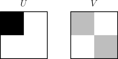
Figure 3.1. Graphons $U$ and $V$ from Example 3.18

The function $f^{*}$ from Example 3.18 is, however, very unnatural since it is not continuous with respect to $L^{1}$ (for a continuous parameter $f$ at least). We leave it as an open problem, whether there is a continuous example.

Problem 3.19.

Is there a graphon parameter $f:\mathcal{W}_{0}\rightarrow\mathbb{R}$ that is not convex, but is continuous in $L^{1}$ and cut distance compatible?

Remark 3.20.

For homomorphism densities $t(H,\cdot):\mathcal{W}_{0}\rightarrow\mathbb{R}$, Theorem 3.17 can be reversed, under the additional assumption that $H$ is a connected graph: $t(H,\cdot)$ is cut distance compatible if and only if it is convex. Let us give details of the direction not covered by Theorem 3.17. Suppose that $t(H,\cdot)$ is cut distance compatible, and $H$ is connected. By Theorem 3.25 below, $H$ is weakly norming. In particular, for the function $f:\mathcal{W}^{+}\rightarrow\mathbb{R}$, $f(U):=t(H,U)^{1/e(H)}$ we have that $f(U_{1}+U_{2})\leq f(U_{1})+f(U_{2})$. Now, for every $\alpha_{1},\alpha_{2},\alpha_{3},\ldots,\alpha_{k}\in[0,1]$ with $\sum_{i}\alpha_{i}=1$ and every graphons $W,W_{1},W_{2},\ldots,W_{k}\in\mathcal{W}_{0}$ with $W=\sum_{i}\alpha_{i}W_{i}$, we have

$$t\left(H,W\right) =f\left(\sum_{i}\alpha_{i}W_{i}\right)^{e(H)}\leq\left(\sum_{i}f\left(\alpha_{i}W_{i}\right)\right)^{e(H)}$$

$$=\left(\sum_{i}\alpha_{i}f\left(W_{i}\right)\right)^{e(H)}\leq\sum_{i}\alpha_{i}\left(f\left(W_{i}\right)\right)^{e(H)}=\sum_{i}\alpha_{i}t\left(H,W_{i}\right)\;,$$

as required.

3.5. Spectrum

The main result in this section, Theorem 3.22, asserts that the spectral quasiorder defined in Section 2.3.4 is a cut distance identifying graphon order. But first we need an easy lemma.

Lemma 3.21.

Let $\left(W_{n}\right)_{n}$ be a sequence of graphons on $\Omega^{2}$ such that $W_{n}\overset{\mathrm{w}^{*}}{\;\longrightarrow\;}U$ for some graphon $U$. Let $u,v\in L^{2}\left(\Omega\right)$. Then we have $\left\langle W_{n}u,v\right\rangle\rightarrow\left\langle Uu,v\right\rangle$.

Proof.

Since step functions are dense in $L^{2}\left(\Omega\right)$, and since the forms $\left\langle W_{n}\cdot,\cdot\right\rangle$ and $\left\langle U\cdot,\cdot\right\rangle$ are obviously bilinear, it suffices to prove the statement for indicator functions of sets, $u=\mathbf{1}_{A}$, $v=\mathbf{1}_{B}$ (where $A,B\subset\Omega$). But in that case $\left\langle W_{n}u,v\right\rangle=\int_{A\times B}W_{n}$ and $\left\langle Uu,v\right\rangle=\int_{A\times B}U$. The statement follows since $W_{n}\overset{\mathrm{w}^{*}}{\;\longrightarrow\;}U$. ∎

We are now ready to prove the main result of this section. Let us note that the arguments that we use to prove this result also turned out to be useful in the setting of finitely forcible graphs; in particular Kráľ, Lovász, Noel, and Sosnovec [24] used our arguments in the final step of their proof that for each graphon and each $\varepsilon>0$, there exists a finitely forcible graphon that differs from the original one only on a set of measure at most $\varepsilon$.

Theorem 3.22.

The spectral quasiorder is a cut distance identifying graphon order. That is, given two graphons $U,W\in\mathcal{W}_{0}$,

1. if $\delta_{\square}(U,W)=0$, then the spectra of $U$ and $W$ are the same, and

2. if $U\prec W$, then $U\stackrel{{\scriptstyle S}}{{\prec}}W$.

Proof.

Part (a) follows from [29, Theorem 11.54].

So, the main work is to prove (b). Consider the sequence $(W^{\pi_{n}})_{n}$ of versions of $W$ such that $W^{\pi_{n}}\overset{\mathrm{w}^{*}}{\;\longrightarrow\;}U$. Let $\lambda_{1}^{+}\geq\lambda_{2}^{+}\geq\lambda_{3}^{+}\geq\ldots\geq 0$ be the positive eigenvalues of $U$ with associated pairwise orthogonal unit eigenvectors $u_{1},u_{2},u_{3},\ldots$, and let $\beta_{1}^{+}\geq\beta_{2}^{+}\geq\beta_{3}^{+}\geq\ldots\geq 0$ be the positive eigenvalues of $W$. First, we will prove that for any given $\varepsilon>0$ and $k$, we have $\beta_{k}^{+}\geq\lambda_{k}^{+}-\varepsilon$. By the maxmin characterization of eigenvalues we have

(3.14) $$\beta_{k}^{+}=\max_{\begin{subarray}{c}H\text{ subspace of }L^{2}(\Omega)\\ \text{dim}(H)=k\end{subarray}}\;\min_{\begin{subarray}{c}g\in H\\ \left\|g\right\|_{2}=1\end{subarray}}\left\langle Wg,g\right\rangle\;.$$

Given $n$, consider the space $\widetilde{H}_{n}=\text{span}\left\{u_{1}^{\pi_{n}^{-1}},u_{2}^{\pi_{n}^{-1}},\ldots,u_{k}^{\pi_{n}^{-1}}\right\}$, where $u_{i}^{\pi_{n}^{-1}}(x)=u_{i}(\pi_{n}^{-1}(x))$. Then (3.14) gives

(3.15) $$\beta_{k}^{+}\geq\min_{\begin{subarray}{c}g\in\widetilde{H}_{n}\\ \left\|g\right\|_{2}=1\end{subarray}}\left\langle Wg,g\right\rangle.$$

Furthermore, by Lemma 3.21 we can find $n$ large enough so that for all $i,j\leq k$ we have

(3.16) $$\left|\left\langle W^{\pi_{n}}u_{i},u_{j}\right\rangle-\left\langle Uu_{i},u_{j}\right\rangle\right|<\frac{\varepsilon}{k^{2}}.$$

Now, for $g\in\widetilde{H}_{n}$ that realizes the minimum in (3.15), we can write its orthogonal decomposition as $g=\sum_{i=1}^{k}c_{i}u_{i}^{\pi_{n}^{-1}}$, where $\sum_{i=1}^{k}c_{i}^{2}=1$. Thus, we obtain

$$\left\langle Wg,g\right\rangle =\left\langle W^{\pi_{n}}g^{\pi_{n}},g^{\pi_{n}}\right\rangle=\left\langle W^{\pi_{n}}\sum_{i=1}^{k}c_{i}u_{i},\sum_{i=1}^{k}c_{i}u_{i}\right\rangle=\sum_{i,j=1}^{k}c_{i}c_{j}\left\langle W^{\pi_{n}}u_{i},u_{j}\right\rangle\;.$$

We can now use (3.16) to replace the terms $\left\langle W^{\pi_{n}}u_{i},u_{j}\right\rangle$ by the terms $\left\langle Uu_{i},u_{j}\right\rangle$,

$$\left\langle Wg,g\right\rangle =\sum_{i=1}^{k}c_{i}^{2}\left(\left\langle Uu_{i},u_{i}\right\rangle\pm\frac{\varepsilon}{k^{2}}\right)+\sum_{\begin{subarray}{c}i,j=1\\ i\neq j\end{subarray}}^{k}c_{i}c_{j}\left(\left\langle Uu_{i},u_{j}\right\rangle\pm\frac{\varepsilon}{k^{2}}\right)$$

$$\geq\sum_{i=1}^{k}c_{i}^{2}\left(\lambda_{i}^{+}-\frac{\varepsilon}{k^{2}}\right)-\sum_{\begin{subarray}{c}i,j=1\\ i\neq j\end{subarray}}^{k}|c_{i}c_{j}|\frac{\varepsilon}{k^{2}}\geq\lambda_{k}^{+}-\varepsilon\;.$$

Thus (3.15) implies $\beta_{k}^{+}\geq\lambda_{k}^{+}-\varepsilon$.

A similar argument can be used for the negative eigenvalues $\lambda_{1}^{-}\leq\lambda_{2}^{-}\leq\lambda_{3}^{-}\leq\ldots\leq 0$ of $U$ and $\beta_{1}^{-}\leq\beta_{2}^{-}\leq\beta_{3}^{-}\leq\ldots\leq 0$ of $W$ to show that $\beta_{k}^{-}\leq\lambda_{k}^{-}+\varepsilon$. That implies $U\stackrel{{\scriptstyle S}}{{\preceq}}W$.

To show that for at least one eigenvalue the corresponding inequality is strict, assume for contradiction that the eigenvalues of $U$ and $W$ are all the same. Then a double application of (2.5) gives

$$\left\|W\right\|_{2}^{2}=\sum\left(\beta_{i}^{+}\right)^{2}+\sum\left(\beta_{i}^{-}\right)^{2}=\sum\left(\lambda_{i}^{+}\right)^{2}+\sum\left(\lambda_{i}^{-}\right)^{2}=\left\|U\right\|_{2}^{2}.$$

But this is a contradiction with Corollary 3.15. This finishes the proof. ∎

3.6. Homomorphism densities

In this section, we address the following problem.

Problem 3.23.

Characterize graphs $H$ for which $t(H,\cdot):\mathcal{W}_{0}\rightarrow\mathbb{R}$ is a cut distance compatible (respectively a cut distance identifying) graphon parameter.

Observe that thanks to Proposition 3.2, for the case of compatible graphon parameters, Problem 3.23 reduces to characterizing graphs $H$ for which we have

(3.17) $$t\left(H,W^{\Join\mathcal{P}}\right) \leq t\left(H,W\right)\text{ for each $W\in\mathcal{W}_{0}$ and each finite partition $\mathcal{P}$}.$$

Similarly, if true, our Conjecture 3.3 implies that for the case of identifying graphon parameters, Problem 3.23 reduces to characterizing graphs $H$ for which we have

(3.18) $$t\left(H,W^{\Join\mathcal{P}}\right) <t\left(H,W\right)\text{ for each $W\in\mathcal{W}_{0}$ and each finite partition $\mathcal{P}$ for which $W\neq W^{\Join\mathcal{P}}$}.$$

This is closely related to Sidorenko’s conjecture (which was asked independently by Simonovits, and by Sidorenko, [36, 35]) and the Forcing conjecture (first hinted in [37, Section 5]). Indeed, these conjectures — when stated in the language of graphons — ask to characterize graphs $H$ for which we have

(3.19) $$t\left(H,W^{\Join\left\{\Omega\right\}}\right) \leq t\left(H,W\right)\text{ for each $W\in\mathcal{W}_{0}$}$$

(Sidorenko’s conjecture), and

(3.20) $$t\left(H,W^{\Join\left\{\Omega\right\}}\right) <t\left(H,W\right)\text{ for each nonconstant $W\in\mathcal{W}_{0}$}$$

$$\text{(Forcing conjecture)}.$$

Recall that Sidorenko’s conjecture asserts that $H$ satisfies (3.19) if and only if $H$ is bipartite. Similarly, the Forcing conjecture asserts that $H$ satisfies (3.20) if and only if $H$ is bipartite and contains a cycle. In both cases, the $\Rightarrow$ direction is easy. Let us recall that the reason why at least one cycle is required for the Forcing conjecture is that the homomorphism density of any forest $H$ in any $p$-regular graphon (whether constant-$p$, or not) is $p^{e(H)}$. The other direction in both conjectures is open, despite being known in many special cases, see [7, 28, 23, 5, 22, 27, 38, 8, 6].

Because all the properties we investigate in this section strengthen (3.19), we are concerned only with bipartite graphs throughout. The only exception is Remark 3.31 which addresses a possible <<converse>> definition of cut distance identifying properties.

Graphs satisfying (3.17) were investigated in [25] where these graphs are said to have the step Sidorenko property. Similarly, graphs satisfying (3.18) are said to have the step forcing property. Clearly, these properties imply (3.19) and (3.20), respectively. These stronger <<step>> properties do not follow automatically from (3.19) and (3.20); in [25, Section 2] it is shown that the 4-cycle with a pendant edge $C_{4}^{+}$ has the Sidorenko property but not the step Sidorenko property. Thus, every graph having the step Sidorenko property must be bipartite and every graph having the step forcing property must be bipartite with a cycle. The focus of [25] was in providing negative examples. For example, it was shown in [25] that a Cartesian product of cycles does not have the step Sidorenko property, unless all the cycles have length 4.

The connection to our running Problem 3.23 comes from Proposition 14.13 of [29] which implies that each weakly norming graph has the step Sidorenko property.

Corollary 3.24.

For each weakly norming graph $H$ the function $t(H,\cdot)$ is cut distance compatible (or, equivalently, $H$ has the step Sidorenko property).

Corollary 3.24 also directly follows from Theorem 3.17. We recall the proof from [29] in Section 3.6.1.

In Section 3.6.2 we prove Theorem 3.25 which states that among connected graphs, the graphs with the step Sidorenko property are exactly the weakly norming graphs (thus answering a question of Kráľ, Martins, Pach and Wrochna [25, Section 5]).

Theorem 3.25.

Suppose that $H$ is a connected graph. If the function $t(H,\cdot)$ is cut distance compatible (or, equivalently, if $H$ has the step Sidorenko property), then $H$ is weakly Hölder.

Remark 3.26.

For disconnected graphs, the statement of Corollary 3.24 actually does not require the graph to be weakly norming, and can be strengthened as follows. If each component $H_{i}$ of a graph $H=H_{1}\sqcup\ldots\sqcup H_{k}$ is weakly norming then $t(H,\cdot)$ is cut distance compatible. Indeed, suppose that $U\preceq W$. Then Corollary 3.24 tells us that for each component, $t(H_{i},U)\leq t(H_{i},W)$. Thus, $t(H,U)=\prod t(H_{i},U)\leq\prod t(H_{i},W)=t(H,W)$, as was needed. We remark, that this relation between weakly norming disconnected graphs and cut distance compatibility might perhaps be an equivalence.

Remark 3.27.

Two nontrivial necessary conditions for a graph $H$ to be weakly Hölder are established in [22, Theorem 2.10]. One of them basically says that $H$ does not contain a subgraph denser than itself. The other condition says that if $V(H)=A_{1}\sqcup A_{2}$ is a bipartition of $H$ and $u,v\in A_{i}$ are two vertices from the same part, then $\deg(u)=\deg(v)$. Thus, Theorem 3.25 restricts quite substantially the class of graphs having the step Sidorenko property, compared to the class of all bipartite graphs which are conjectured to have the Sidorenko property. In particular, we see directly that $C_{4}^{+}$ does not have the step Sidorenko property.

The next theorem, which we prove in Section 3.6.3, is our another main result.

Theorem 3.28.

Suppose that $H$ is a norming graph. Then the parameter $t(H,\cdot)$ is cut distance identifying. In particular, by the trivial direction of Conjecture 3.3, $H$ is step forcing.

Note that Theorem 3.28 is an implication only. It is reasonable to ask about the converse (for connected graphs, for the same reasons as in Remark 3.26).

Problem 3.29.

Is it true that if a connected graph $H$ has the step forcing property (or if $t(H,\cdot)$ is cut distance identifying, which may be a more restrictive assumption), we also have that $H$ is norming?

Before showing the proofs of Theorem 3.25 and Theorem 3.28, we summarize in Figure 3.2 the known and conjectured relations for weakly norming graphs, norming graphs, graphs with the step Sidorenko or the step forcing property, and graphs that give cut distance compatible or cut distance identifying parameters.

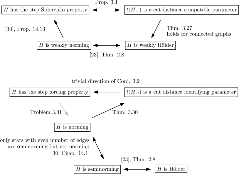
Figure 3.2. Diagram of notions regarding homomorphism densities used in this paper and their relations.

3.6.1. Proof of Corollary 3.24

Here, we prove that each weakly norming graph $H$ has the step Sidorenko property. Our argument is a tailored version of the proof of Proposition 14.13 of [29] (where the statement is proven in bigger generality, for so-called smooth invariant norms). The reason why we recall this argument is that it will allow us to understand the strategy for proving Theorem 3.28, as we explain at the end of this section.

So, suppose that $H$ is a weakly norming graph, $W:\Omega^{2}\rightarrow[0,1]$ is a graphon, $\mathcal{P}$ is a finite partition of $\Omega$. We need to prove that $t\left(H,W\right)\geq t\left(H,W^{\Join\mathcal{P}}\right)$. Without loss of generality, we can assume that $\Omega=[0,1)$ (see Remark 2.4), and that $\mathcal{P}$ is a partition into intervals $\left\{[a_{\ell},a_{\ell+1})\right\}_{\ell=1}^{|\mathcal{P}|}$. Fix a number $\eta$ which is irrational with respect to the lengths of all the intervals $[a_{\ell},a_{\ell+1})$. Consider the map $\gamma:[0,1)\rightarrow[0,1)$ that maps each number $x\in[0,1)$, say $x\in[a_{i},a_{i+1})$, to $\left((x-a_{i}+\eta)\right)\mod(a_{i+1}-a_{i})+a_{i}$. Clearly, the map $\gamma$ is a measure preserving bijection on $[0,1)$, where each interval $[a_{\ell},a_{\ell+1})$ is $\gamma$-invariant, and $\gamma$ restricted to each $[a_{\ell},a_{\ell+1})$ is ergodic. It follows that the map $\left(x,y\right)\mapsto\left(\gamma(x),\gamma(y)\right)$ is ergodic when restricted on each set of the form $[a_{\ell},a_{\ell+1})\times[a_{k},a_{k+1})$.

For $n\in\mathbb{N}$, let $U_{n}$ be the version of $W$ obtained using the $n$-th iteration of $\gamma$, $U_{n}:=W^{\gamma^{n}}$. For $n\in\mathbb{N}$, let $S_{n}:=\frac{1}{n}\sum_{k=1}^{n}U_{k}$. The Pointwise Ergodic Theorem tells us that the graphons $S_{n}$ converge pointwise to $W^{\Join\mathcal{P}}$. Hence,

$$\sqrt[e(H)]{t\left(H,W^{\Join\mathcal{P}}\right)} =\lim_{n\rightarrow\infty}\sqrt[e(H)]{t\left(H,S_{n}\right)}=\lim_{n\rightarrow\infty}\sqrt[e(H)]{t\left(H,\frac{1}{n}\sum_{k=1}^{n}U_{k}\right)}$$

$$\sqrt[e(H)]{t\left(H,|\cdot|\right)} \leq\lim_{n\rightarrow\infty}\frac{1}{n}\cdot\sum_{k=1}^{n}\sqrt[e(H)]{t\left(H,U_{k}\right)}$$ is a seminorm

$$t\left(H,U_{k}\right)=t\left(H,W\right) =\sqrt[e(H)]{t\left(H,W\right)}\;,$$

as was needed. This finishes the proof of Corollary 3.24.

Let us now look back at the argument to see what needs to be strengthened to give Theorem 3.28. Actually, in this informal sketch, we only want to show that $H$ is step forcing, rather than $t(H,\cdot)$ being cut distance identifying.

That is, we have a norming graph $H$, a graphon $W:\Omega^{2}\rightarrow[0,1]$, a finite partition $\mathcal{P}$ of $\Omega$, such that $W\neq W^{\Join\mathcal{P}}$. We need to prove that $t\left(H,W\right)>t\left(H,W^{\Join\mathcal{P}}\right)$. The only space for getting the needed strict inequality in the calculation above is in the triangle inequality on the second line. In view of Remark 2.1, and using the fact that $H$ is norming and hence $\left\|\cdot\right\|_{H}$ uniformly convex by Theorem 2.16, it only remains to argue that many of the graphons $U_{k}$ are far from colinear, where <<far from colinear>> is measured in the $\left\|\cdot\right\|_{H}$-norm. This is indeed plausible: since $W\neq W^{\Join\mathcal{P}}$, the graphons $U_{k}$ must indeed be different.

As we shall see in Section 3.6.3, there are several difficulties in the actual proof of Theorem 3.28. In particular, we were not able to show that this approach works with $U_{k}=W^{\gamma^{k}}$, and needed to choose the approximating graphons $U_{k}$ with the help of (rather technical) Lemma 2.24.

3.6.2. Proof of Theorem 3.25

Let $H$ be a connected graph such that $t(H,\cdot)$ is cut distance compatible. Suppose that $H$ has $m$ edges and $n$ vertices. We prove that $H$ is weakly Hölder. By Theorem 2.14 we already know that weakly Hölder graphs are exactly weakly norming graphs. We divide the proof of the theorem into two parts. At first we prove that $t(H,\cdot)$ is subadditive up to a constant loss, specifically, we show that

(3.21) $$t(H,U)^{1/m}+t(H,V)^{1/m} \geq\frac{1}{4}\cdot t(H,U+V)^{1/m}\;.$$

Then we use this inequality to prove that $H$ is weakly norming using the tensoring technique in the same way as it is used in the proof of Theorem 2.8 from [22].

Let $U$ and $V$ be two arbitrary graphons and let $W_{1}$ be a graphon containing a copy of $U$ scaled by the factor of one half in its top-left corner (i.e., $W_{1}\left(x,y\right)=U\left(2x,2y\right)$ for $(x,y)\in[0,\frac{1}{2}]^{2}$), a copy of $V$ in its bottom-right corner (i.e., $W_{1}\left(x,y\right)=V\left(2(x-\frac{1}{2}),2(y-\frac{1}{2})\right)$ for $(x,y)\in[\frac{1}{2},1]^{2}$), and zero otherwise (see Figure 3.3). Note that for the homomorphism density $t(H,W_{1})$ we have

$$t(H,W_{1}) =\frac{t(H,U)+t(H,V)}{2^{n}}\;.$$

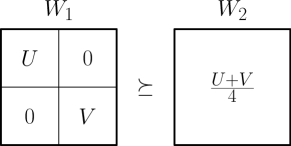
Figure 3.3. Graphons $U$, $V$, $W_{1}$ and $W_{2}$ from the proof of Theorem 3.25

This is because $H$ is connected and, thus, homomorphisms that map a positive number of vertices of $H$ to $[0,\frac{1}{2}]$, and a positive number of vertices to $[\frac{1}{2},1]$ do not contribute to the value of the integral $t(H,W_{1})$. Now consider the graphon $W_{2}=\frac{U+V}{4}$. By [12, Lemma 4.2] we have $W_{1}\succeq W_{2}$. It follows that $t(H,W_{1})\geq t(H,W_{2})$. Observe that $t(H,W_{2})=t\left(H,\frac{U+V}{4}\right)=\frac{t(H,U+V)}{4^{m}}$, hence we get

$$\frac{t(H,U)+t(H,V)}{2^{n}} \geq\frac{t(H,U+V)}{4^{m}}\;.$$

We are actually interested in the quantity $t(H,U)^{1/m}$, so we rewrite this as

$$\left(t(H,U)+t(H,V)\right)^{1/m} \geq\frac{2^{n/m}}{4}\cdot t(H,U+V)^{1/m}\geq\frac{1}{4}\cdot t(H,U+V)^{1/m}\;.$$

Finally note that $t(H,U)^{1/m}+t(H,V)^{1/m}\geq\left(t(H,U)+t(H,V)\right)^{1/m}$, as can be verified by raising the inequality to the $m$-th power. This yields the desired inequality (3.21).

Now we need to improve the constant on the right-hand side of (3.21). To this end we use the tensor power trick in the same way as was used in [22, Theorem 2.8] and in [29, Theorem 14.1].

Note that the inequality (3.21) can be inductively generalised to yield that for a sequence of graphons $U_{1},\dots,U_{\ell}$ we have

(3.22) $$\sum_{i=1}^{\ell}t(H,U_{i})^{1/m} \geq\left(\frac{1}{4}\right)^{\ell-1}\cdot t\left(H,\sum_{i=1}^{\ell}U_{i}\right)^{1/m}.$$

Let $(H,w)$ be a $\mathcal{W}^{+}$-decoration of $H$. By Lemma 2.12 we may assume that $t(H,W_{e})=1$ for every $W_{e}$. We want to prove that $t(H,w)\leq 1$, but at first we prove the weaker inequality $t(H,w)\leq 4^{m(m-1)}\cdot m^{m}$. We have

(3.23) $$t(H,w) \leq t\left(H,\sum_{e\in E(H)}W_{e}\right)\leq\left(4^{m-1}\cdot\sum_{e\in E(H)}t(H,W_{e})^{1/m}\right)^{m}=4^{m(m-1)}\cdot m^{m}\;,$$

where in the first inequality we replaced each $W_{e}$ by $\sum_{e\in E(H)}W_{e}$, while the second inequality is due to the bound (3.22). Now suppose that we decorate each edge $e$ of $H$ by $W_{e}^{\otimes k}$ for $k\geq 1$. As we observed in (2.4) and (2.3), we then have $t\left(H,w^{\otimes k}\right)=t(H,w)^{k}$ and $t\left(H,W_{e}^{\otimes k}\right)=t\left(H,W_{e}\right)^{k}=1$. Thus inequality (3.23) gives that $t(H,w)^{k}=t(H,w^{\otimes k})\leq 4^{m(m-1)}\cdot m^{m}$, thus $t(H,w)\leq\left(4^{m(m-1)}\cdot m^{m}\right)^{1/k}$. Since this holds for any $k\geq 1$, we conclude that $t(H,w)\leq 1$.

3.6.3. Proof of Theorem 3.28

Let $H$ be a norming graph. By Fact 2.13, it is enough to consider the case that $H$ is connected. Suppose that $H$ has $m$ edges. Since $m>1$ (cf. Fact 2.11(b)), we know from Section 2.4.1 that the modulus of convexity $\mathfrak{d}_{H}$ of the norm $\left\|\cdot\right\|_{H}$ defined by (2.10) is strictly positive.

Suppose that $U,V\in\mathcal{W}^{+}$ are such that $V\prec U$. We want to prove that $t(H,U)>t(H,V)$. Clearly, we may assume that $t(H,V)>0$. By rescaling, we may moreover assume that $t(H,U)=1$. Let us define $\delta:=\frac{\delta_{\square}(U,V)}{32}$. We now set

$$\xi:=\min\big{(}\mathfrak{d}_{H}\left(\delta\right),\|V\|_{H}\big{)}\quad\text{and}\quad\varepsilon:=\frac{1}{4m\cdot\left\|U\right\|_{\infty}^{m-1}}\cdot\left(\frac{1}{10}\cdot\xi\right)^{m}\;.$$

Let an even number $N$ and measure preserving bijections $\left(\phi_{i}\right)_{i=1}^{N}$ be given by Lemma 2.24 (see also Remark 2.25) for the inputs $U$ and $V$. Since $V\preceq U$, we have $\left\|V\right\|_{\infty}\leq\left\|U\right\|_{\infty}.$ Since $\left\|V-\frac{\sum_{i=1}^{N}U^{\phi_{i}}}{N}\right\|_{1}<\varepsilon$, we have

(3.24) $$\left|t\left(H,\frac{\sum_{i=1}^{N}U^{\phi_{i}}}{N}\right)-t(H,V)\right| \overset{L\ref{lem:countinglemma}}{\leq}4m\cdot\left\|U\right\|_{\infty}^{m-1}\cdot\delta_{\square}\left(\frac{\sum_{i=1}^{N}U^{\phi_{i}}}{N},V\right)$$

$$\leq 4m\cdot\left\|U\right\|_{\infty}^{m-1}\cdot\left\|V-\frac{\sum_{i=1}^{N}U^{\phi_{i}}}{N}\right\|_{1}<\left(\frac{\xi}{10}\right)^{m}\;.$$

Observe that for each index $i\in\left\{1,2,\ldots,\frac{N}{2}\right\}$ that satisfies (2.18), an application of Proposition 2.15 to the kernel $X:=U^{\phi_{2i-1}}-U^{\phi_{2i}}$ gives that

$$\|U^{\phi_{2i-1}}-U^{\phi_{2i}}\|_{H}\geq\|U^{\phi_{2i-1}}-U^{\phi_{2i}}\|_{\square}\geq\delta\;.$$

Since $\left\|U\right\|_{H}=1$, any two versions of $U$ that are far apart can play the role of $x$ and $y$ in (2.1). Thus, if we have an index $i\in\left\{1,2,\ldots,\frac{N}{2}\right\}$ that satisfies (2.18), then we get that

$$1-\sqrt[m]{t\left(H,\frac{U^{\phi_{2i-1}}+U^{\phi_{2i}}}{2}\right)}\geq\mathfrak{d}_{H}\left(\delta\right)\geq\xi.$$

Since $t(H,U)=1$, we may equivalently write

(3.25) $$\sqrt[m]{t(H,U^{\phi_{2i-1}})}+\sqrt[m]{t(H,U^{\phi_{2i}})} \geq\sqrt[m]{t(H,U^{\phi_{2i-1}}+U^{\phi_{2i}})}+2\xi\;.$$

We are now in a position to do the the final calculation. We have

(3.26) $$\sqrt[m]{t(H,U)}=\frac{1}{N}\left(\sqrt[m]{t\left(H,U^{\phi_{1}}\right)}+\sqrt[m]{t\left(H,U^{\phi_{2}}\right)}+\dots+\sqrt[m]{t\left(H,U^{\phi_{N}}\right)}\right)\;.$$

Let us now group the summands on the right-hand side of (3.26) into $\frac{N}{2}$ pairs $\sqrt[m]{t\left(H,U^{\phi_{2i-1}}\right)}+\sqrt[m]{t\left(H,U^{\phi_{2i}}\right)}$. Either a given pair satisfies (3.25), or, if not, the subadditivity of $\left\|\cdot\right\|_{H}$ gives us somewhat weaker $\sqrt[m]{t(H,U^{\phi_{2i-1}})}+\sqrt[m]{t(H,U^{\phi_{2i}})}\geq\sqrt[m]{t(H,U^{\phi_{2i-1}}+U^{\phi_{2i}})}$. Recall that at least $\frac{N}{4}$ pairs satisfy (3.25). Thus,

$$\sqrt[m]{t(H,U)} \geq\frac{1}{N}\left(\sqrt[m]{t\left(H,U^{\phi_{1}}+U^{\phi_{2}}\right)}+\dots+\sqrt[m]{t\left(H,U^{\phi_{N-1}}+U^{\phi_{N}}\right)}+\frac{N}{4}\cdot 2\xi\right)$$

subadditivity of $$\left\|\cdot\right\|_{H} \geq\frac{1}{N}\sqrt[m]{t\left(H,U^{\phi_{1}}+U^{\phi_{2}}+\dots+U^{\phi_{N}}\right)}+\frac{\xi}{2}$$

$$=\sqrt[m]{t\left(H,\frac{\sum_{i=1}^{N}U^{\phi_{i}}}{N}\right)}+\frac{\xi}{2}$$

by (3.24); $$t(H,V)>(\frac{\xi}{10})^{m} \geq\sqrt[m]{t(H,V)-\big{(}\frac{\xi}{10}\big{)}^{m}}+\frac{\xi}{2}$$

$$\geq\sqrt[m]{t(H,V)}-\frac{\xi}{10}+\frac{\xi}{2}$$

$$>\sqrt[m]{t(H,V)}\;,$$

as was needed.

3.6.4. Discussion

Remark 3.30.

Let us comment on the role of the abstract weak* approach we introduced in [12] in our proofs of Theorem 3.25 and Theorem 3.28.

• In Theorem 3.25 we deduced the property of being weakly Hölder by using inequalities of the form $t(H,W_{1})\geq t(H,W_{2})$, where $W_{1}$ and $W_{2}$ are constructed from graphons $U$ and $V$ as in Figure 3.3. These inequalities follow from the fact that $W_{1}\succeq W_{2}$; but we do not have that $W_{2}$ is a stepping of $W_{1}$. In other words, the immediate property of $H$ we use is that $t(H,\cdot)$ is cut distance compatible, rather than $H$ having the step Sidorenko property. (Of course, the two properties are equivalent, by Proposition 3.2.) So, the weak* approach and the notion of the structuredness order were instrumental here.

• Theorem 3.28 cannot be even stated without the notion of the structuredness order (until the validity of Conjecture 3.3 is confirmed). On the other hand, a version of Theorem 3.28 which would not use the structuredness order, <<Suppose that $H$ is a norming graph. Then $H$ is step forcing.>> is either equivalent (if Conjecture 3.3 holds), or only a tiny bit weaker. Our proof of Theorem 3.28 could then be easily modified so that it avoids any notions introduced in [12], that is using only traditional technology available after Hatami [22]. Actually, in this setting it would be enough to prove Lemma 2.24 for $V=U^{\Join\mathcal{P}}$ rather than $V\prec U$, which would result in a proof of that lemma shorter by one or two pages.

Remark 3.31.

Note that the definition of cut distance compatible (resp. identifying) parameters given at the beginning of Section 3.1 was somewhat arbitrary. That is, instead of requiring that $W_{1}\preceq W_{2}$ implies $\theta\left(W_{1}\right)\leq\theta\left(W_{2}\right)$ (resp. that $W_{1}\prec W_{2}$ implies $\theta\left(W_{1}\right)<\theta\left(W_{2}\right)$), we could have reversed the inequalities to $\theta\left(W_{1}\right)\geq\theta\left(W_{2}\right)$ (resp. $\theta\left(W_{1}\right)>\theta\left(W_{2}\right)$). However, among graphon parameters induced by graph densities, there are only trivial examples of cut distance compatible parameters in this sense. These correspond to the graphs that are disjoint unions of cliques on 1 and 2 vertices. For these graphs the homomorphism densities are either always constant 1 (if the graph is a disjoint union of vertices), or the power of the edge density of the graph (otherwise). Since we know that $U\succeq V$ implies that the edge densities of the two graphons are the same (Fact 2.20), these examples are cut distance compatible parameters in both senses for a trivial reason, and, in particular, they are not cut distance identifying parameters in this reverse sense. To see that there are no other examples of cut distance compatible parameters in the reverse sense, consider the two following graphons: a graphon $W_{\mathrm{clique}}$ consisting of a clique of measure $0.5$ ($W_{\mathrm{clique}}(x,y)=1$ if and only if $0\leq x,y\leq\frac{1}{2}$ and $W_{\mathrm{clique}}(x,y)=0$ otherwise), and the constant graphon $W_{\mathrm{const}}\equiv\frac{1}{4}$. Now let $H$ be a graph that is not a disjoint union of cliques of order one or two. Without loss of generality we may assume that $H$ does not contain any component consisting of a single vertex. Hence $2e(H)>v(H)$. Now we have $W_{\mathrm{const}}\preceq W_{\mathrm{clique}}$, but $t\left(H,W_{\mathrm{const}}\right)=\left(\frac{1}{4}\right)^{e(H)}<\left(\frac{1}{2}\right)^{v(H)}=t\left(H,W_{\mathrm{clique}}\right)$.

3.6.5. Local Sidorenko’s conjecture

An interesting weakening of Sidorenko’s conjecture is to require (3.19) only for graphons $W$ that are close to a constant graphon. More precisely, we say that a graph $H$ has the local Sidorenko property with respect to the $L^{1}$-norm (resp. with respect to the cut norm or with respect to the $L^{\infty}$-norm) if for each $p\in\left[0,1\right]$ there exists an $\varepsilon>0$ such that for each graphon $W$ of edge density $p$ and with $\left\|W-p\right\|_{1}<\varepsilon$ (resp. with $\left\|W-p\right\|_{\square}<\varepsilon$ or with $\left\|W-p\right\|_{\infty}<\varepsilon$) we have that $t(H,W)\geq p^{e(H)}$. This weakening was first considered by Lovász [28] who proved that bipartite graphs are indeed locally Sidorenko (even with respect to the cut norm, which is the strongest of the results). Recently a full characterization of graphs with the local Sidorenko was announced by Fox and Wei [16]: a graph is locally Sidorenko if and only if it is a forest or has even girth.

We can combine the <<step>> and the <<local>> features in an obvious way. We say that a graph $H$ has the local step Sidorenko property if for each partition $\mathcal{P}=\left(\Omega_{i}\right)_{i=1}^{k}$ of $\Omega$ and each template of densities $\left(p_{ij}\in[0,1]\right)_{i,j\in[k]}$ there exists $\varepsilon>0$ such that for each graphon $W$ for which the average of $W$ on each $\Omega_{i}\times\Omega_{j}$ equals $p_{ij}$, and for which $W^{\Join\mathcal{P}}$ is $\varepsilon$-close to $W$ in some fixed norm as above, we have $t\left(H,W^{\Join\mathcal{P}}\right)\leq t\left(H,W\right)$. Locally step forcing graphs can be defined analogously.

Problem 3.32.

Characterize locally step Sidorenko and locally step forcing graphs (with respect to the norms $\left\|\cdot\right\|_{1}$, $\left\|\cdot\right\|_{\square}$, or $\left\|\cdot\right\|_{\infty}$).

3.6.6. Two positive results directly

We conclude the treatment of Problem 3.23 by two positive results, namely that stars are step Sidorenko and that even cycles are step forcing. Propositions 3.33 and 3.34 in the case $\ell=2$ are not new and follow from the results on weakly norming and Hölder graphs above. Yet, the short proofs given here nicely employ other parts of the theory established in this paper.

Proposition 3.33.

For each $\ell\in\mathbb{N}$, the graphon parameter $t\left(K_{1,\ell},\cdot\right):\mathcal{W}_{0}\rightarrow\mathbb{R}$ is cut distance compatible.

Proof.

The key is to observe that for a graphon $\Gamma$, we have $t\left(K_{1,\ell},\Gamma\right)=\int_{x\in\left[0,1\right]}x^{\ell}\mathrm{d}\boldsymbol{\Upsilon}_{\Gamma}$, where $\boldsymbol{\Upsilon}_{\Gamma}$ is defined by (2.13). So, suppose that $U\preceq W$. By Proposition 2.22, we have that $\boldsymbol{\Upsilon}_{U}$ is at least as flat as $\boldsymbol{\Upsilon}_{W}$. Let $\Lambda$ be the measure on $\left[0,1\right]^{2}$ as in Definition 2.21 that witnesses this. In the following inequality, the measures $\Lambda_{x}^{1}$, $x\in[0,1]$, are given by the disintegration of the measure $\Lambda$ on the first coordinate; see [12, p. 272] for a formal definition. We have

$$t\left(K_{1,\ell},U\right) =\int_{x\in\left[0,1\right]}x^{\ell}\mathrm{d}\boldsymbol{\Upsilon}_{U}$$

by Lemma 4.12 from [12] $$=\int_{x\in[0,1]}\left(\int_{y\in[0,1]}y\>\mathrm{d}\Lambda_{x}^{1}\right)^{\ell}\>\mathrm{d}\boldsymbol{\Upsilon}_{U}$$

Jensen’s inequality $$\leq\int_{x\in[0,1]}\int_{y\in[0,1]}y^{\ell}\>\mathrm{d}\Lambda_{x}^{1}\>\mathrm{d}\boldsymbol{\Upsilon}_{U}$$

definition of disintegration $$=\int_{(x,y)\in[0,1]^{2}}y^{\ell}\>\mathrm{d}\Lambda$$

$$=\int_{y\in[0,1]}y^{\ell}\>\mathrm{d}\boldsymbol{\Upsilon}_{W}$$

$$=t\left(K_{1,\ell},W\right)\;.$$

∎

Proposition 3.34.

For each $\ell\in\left\{2,3,4,\ldots\right\}$, the graphon parameter $t\left(C_{2\ell},\cdot\right):\mathcal{W}_{0}\rightarrow\mathbb{R}$ is cut distance identifying.

Before giving a proof, let us note that Lemma 11 in [10] is equivalent to the case $\ell=2$ of the proposition. However, the proof in [10] does not seem to generalize to any higher $\ell$, in which case Proposition 3.34 seems to be new.

Proof of Proposition 3.34.

To prove the proposition, suppose that $\ell$ is fixed and $W_{1}\prec W_{2}$ are two graphons. Theorem 3.22 tells us that $W_{1}\stackrel{{\scriptstyle S}}{{\prec}}W_{2}$. That is, the sum of the $\left(2\ell\right)$-th powers of eigenvalues of $W_{1}$ is strictly smaller than that of $W_{2}$. The statement now follows from Equation (2.6). ∎

3.6.7. A recent result of Lee and Schülke

Combining Theorem 3.17 and Remark 3.20 (see also Figure 3.2), we get that for a connected graph $H$ the function $t(H,\cdot)$ is convex on $\mathcal{W}_{0}$ if and only if $H$ is weakly norming. A direct proof of this equivalence, together with a counterpart equivalence of the convexity of $t(H,\cdot)$ on $\mathcal{W}$ and $H$ being norming was proven in [26]. These equivalences are then used in [26] to argue that $K_{5,5}\setminus C_{10}$ (one of the smallest graphs where Sidorenko’s conjecture is open) is not weakly norming, and that $K_{t,t}$ minus a perfect matching is not norming.

4. Conclusion and possible further directions

In this paper, we studied cut distance identifying and cut distance compatible graphon parameters and graphon orders. This was based on the structuredness order $\preceq$ introduced in [12]. The basic theory of the structurdness order and the key fact that $\preceq$-maximal elements in the space of weak* limits are actually cut-distance limits readily translate to some other combinatorial-analytic objects such as kernels (that is, we allow even negative values), or digraphons (limits of directed graphons, i.e., not necessarily symmetric measurable functions $D:\Omega^{2}\rightarrow[0,1]$), and so does the main feature of the pushforward measures expressed in Proposition 2.22. We think it would be interesting to investigate cut distance identifying/compatible parameters for these structures. For example, for digraph(on)s, there is a reasonable theory of quasirandomness (see [20] and references therein), and, as we saw, characterizing quasirandomness is in a sense dual to characterizing $\preceq$-maximal elements in the space of weak* limits.

The same program could be attempted for limits of $k$-uniform hypergraphs. However, already the basic theory of the weak* approach to hypergraphons seems to be substantially more involved (work in progress). Also, note that the transition from graphon parameters to hypergraphon parameters will not be automatic at all; for example, the Sidorenko conjecture does not have a reasonable counterpart for hypergraphons (see [38]).

References

• [1] N. Alon and J. H. Spencer. The probabilistic method. Wiley-Interscience Series in Discrete Mathematics and Optimization. John Wiley & Sons Inc., Hoboken, NJ, third edition, 2008. With an appendix on the life and work of Paul Erdős.
• [2] T. Austin. On exchangeable random variables and the statistics of large graphs and hypergraphs. Probab. Surv., 5:80–145, 2008.
• [3] C. Borgs, J. T. Chayes, L. Lovász, V. T. Sós, and K. Vesztergombi. Convergent sequences of dense graphs. I. Subgraph frequencies, metric properties and testing. Adv. Math., 219(6):1801–1851, 2008.
• [4] F. R. K. Chung, R. L. Graham, and R. M. Wilson. Quasi-random graphs. Combinatorica, 9(4):345–362, 1989.
• [5] D. Conlon, J. Fox, and B. Sudakov. An approximate version of Sidorenko’s conjecture. Geom. Funct. Anal., 20(6):1354–1366, 2010.
• [6] D. Conlon, J. H. Kim, C. Lee, and J. Lee. Some advances on Sidorenko’s conjecture. J. Lond. Math. Soc. (2), 98(3):593–608, 2018.
• [7] D. Conlon and J. Lee. Finite reflection groups and graph norms. Adv. Math., 315:130–165, 2017.
• [8] D. Conlon and J. Lee. Sidorenko’s conjecture for blow-ups. Discrete Anal., pages 1–13 (paper no. 2), 2021.
• [9] J. W. Cooper, T. Kaiser, D. Král’, and J. A. Noel. Weak regularity and finitely forcible graph limits. Trans. Amer. Math. Soc., 370(6):3833–3864, 2018.
• [10] J. W. Cooper, D. Kral, and T. L. Martins. Finitely forcible graph limits are universal. Adv. Math., 340:819–854, 2018.
• [11] P. Diaconis and S. Janson. Graph limits and exchangeable random graphs. Rend. Mat. Appl. (7), 28(1):33–61, 2008.
• [12] M. Doležal, J. Grebík, J. Hladký, I. Rocha, and V. Rozhoň. Relating the cut distance and the weak* topology for graphons. J. Combin. Theory Ser. B, 147:252–298, 2021.
• [13] J. Doležal, M. Hladký. Cut-norm and entropy minimization over weak* limits. J. Combin. Theory Ser. B, 137:232–263, 2019.
• [14] G. Elek and B. Szegedy. A measure-theoretic approach to the theory of dense hypergraphs. Adv. Math., 231(3-4):1731–1772, 2012.
• [15] P. Erdős and M. Simonovits. Supersaturated graphs and hypergraphs. Combinatorica, 3(2):181–192, 1983.
• [16] J. Fox and F. Wei. On the local approach to Sidorenko’s conjecture. In European Conference on Combinatorics, Graph Theory and Applications (EuroComb 2017), volume 61 of Electron. Notes Discrete Math., pages 459–465. Elsevier Sci. B. V., Amsterdam, 2017.
• [17] A. Frieze and R. Kannan. Quick Approximation to Matrices and Applications. Combinatorica, 19(2):175–220, 1999.
• [18] F. Garbe, J. Hladký, and J. Lee. Two remarks on graph norms. Discrete Comput. Geom. (2021), https://doi.org/10.1007/s00454-021-00280-w.
• [19] W. T. Gowers. Hypergraph regularity and the multidimensional Szemerédi theorem. Ann. of Math. (2), 166(3):897–946, 2007.
• [20] S. Griffiths. Quasi-random oriented graphs. J. Graph Theory, 74(2):198–209, 2013.
• [21] O. Hanner. On the uniform convexity of $L^{p}$ and $l^{p}$. Ark. Mat., 3:239–244, 1956.
• [22] H. Hatami. Graph norms and Sidorenko’s conjecture. Israel J. Math., 175:125–150, 2010.
• [23] J. H. Kim, C. Lee, and J. Lee. Two approaches to Sidorenko’s conjecture. Trans. Amer. Math. Soc., 368(7):5057–5074, 2016.
• [24] D. Král’, L. M. Lovász, J. A. Noel, and J. Sosnovec. Finitely forcible graphons with an almost arbitrary structure. Discrete Anal., pages 1–36 (paper no. 9), 2020.
• [25] D. Král’, T. Martins, P. P. Pach, and M. Wrochna. The step Sidorenko property and non-norming edge-transitive graphs. J. Combin. Theory Ser. A, 162:34–54, 2019.
• [26] J. Lee and B. Schülke. Convex graphon parameters and graph norms. Israel J. Math., 242(2):549–563, 2021.
• [27] J. L. X. Li and B. Szegedy. On the logarithimic calculus and Sidorenko’s conjecture. arXiv:1107.1153.
• [28] L. Lovász. Subgraph densities in signed graphons and the local Simonovits-Sidorenko conjecture. Electron. J. Combin., 18(1):Paper 127, 21, 2011.
• [29] L. Lovász. Large networks and graph limits, volume 60 of American Mathematical Society Colloquium Publications. American Mathematical Society, Providence, RI, 2012.
• [30] L. Lovász and B. Szegedy. Limits of dense graph sequences. J. Combin. Theory Ser. B, 96(6):933–957, 2006.
• [31] L. Lovász and B. Szegedy. Szemerédi’s Lemma for the analyst. J. Geom. and Func. Anal, 17:252–270, 2007.
• [32] C. McDiarmid. On the method of bounded differences. In Surveys in combinatorics, 1989 (Norwich, 1989), volume 141 of London Math. Soc. Lecture Note Ser., pages 148–188. Cambridge Univ. Press, Cambridge, 1989.
• [33] G. Regts and A. Schrijver. Compact orbit spaces in Hilbert spaces and limits of edge-colouring models. European J. Combin., 52(part B):389–395, 2016.
• [34] A. Scott. Szemerédi’s regularity lemma for matrices and sparse graphs. Combin. Probab. Comput., 20(3):455–466, 2011.
• [35] A. Sidorenko. A correlation inequality for bipartite graphs. Graphs Combin., 9(2):201–204, 1993.
• [36] M. Simonovits. Extremal graph problems, degenerate extremal problems, and supersaturated graphs. In Progress in graph theory (Waterloo, Ont., 1982), pages 419–437. Academic Press, Toronto, ON, 1984.
• [37] J. Skokan and L. Thoma. Bipartite subgraphs and quasi-randomness. Graphs Combin., 20(2):255–262, 2004.
• [38] B. Szegedy. An information theoretic approach to Sidorenko’s conjecture. arXiv:1406.6738.
• [39] E. Szemerédi. Regular partitions of graphs. In Problèmes combinatoires et théorie des graphes (Colloq. Internat. CNRS, Univ. Orsay, Orsay, 1976), volume 260 of Colloq. Internat. CNRS, pages 399–401. CNRS, Paris, 1978.