Laplacian preconditioning of elliptic PDEs: Localization of the eigenvalues of the discretized operator

Abstract

In the paper Preconditioning by inverting the Laplacian; an analysis of the eigenvalues. IMA Journal of Numerical Analysis 29, 1 (2009), 24–42, Nielsen, Hackbusch and Tveito study the operator generated by using the inverse of the Laplacian as preconditioner for second order elliptic PDEs $\nabla\cdot(k(x)\nabla u)=f$. They prove that the range of $k(x)$ is contained in the spectrum of the preconditioned operator, provided that $k$ is continuous. Their rigorous analysis only addresses mappings defined on infinite dimensional spaces, but the numerical experiments in the paper suggest that a similar property holds in the discrete case. Motivated by this investigation, we analyze the eigenvalues of the matrix $\bf{L}^{-1}\bf{A}$, where $\bf{L}$ and ${\bf{A}}$ are the stiffness matrices associated with the Laplace operator and general second order elliptic operators, respectively. Without any assumption about the continuity of $k(x)$, we prove the existence of a one-to-one pairing between the eigenvalues of $\bf{L}^{-1}\bf{A}$ and the intervals determined by the images under $k(x)$ of the supports of the FE nodal basis functions. As a consequence, we can show that the nodal values of $k(x)$ yield accurate approximations of the eigenvalues of $\bf{L}^{-1}\bf{A}$. Our theoretical results are illuminated by several numerical experiments.

65F08, 65F15, 65N12, 35J99

1 Introduction

The classical analysis of Krylov subspace solvers for matrix problems with Hermitian matrices relies on their spectral properties; see, e.g., [1, 15]. Typically one seeks a preconditioner which yields parameter independent bounds for the extreme eigenvalues; see, e.g., [8, 18, 25, 14, 24] for a discussion of this issue in terms of operator preconditioning. This approach has the advantage that only the largest and smallest eigenvalues (in the absolute sense if an indefinite problem is solved) must be studied, and the bounds for the required number of Krylov subspace iterations can become independent of the mesh size and other important parameters. This is certainly of great importance, but it does not automatically represent a solution to the challenge of identifying efficient preconditioning. Efficiency of the preconditioning in this approach requires that the convergence bounds based on a single number characteristics, such as the condition number, guarantee sufficient accuracy of the computed approximation to the solution within an acceptable number of iterations.

Since Krylov subspace methods are strongly nonlinear in the input data (matrix and the initial residual), more information about the spectrum is needed in order to capture the actual convergence behavior with its desirable superlinear character. This has been pointed out by several studies [2, 3, 19, 20, 35, 29], and the acceleration of the convergence of the method of conjugate gradients (CG) has been linked with the presence of large outlying eigenvalues and clustering of the eigenvalues. Since Krylov subspace methods for systems with Hermitian matrices use short recurrences, exact arithmetic considerations must be complemented with a thorough rounding error analysis, otherwise it can in practice be misleading or even completely useless. The deterioration of convergence due to rounding errors in the presence of large outlying eigenvalues has been reported, based on experiments, already in [21]; see also [7], [19, p. 72], the discussion in [35, p. 559] and the summary in [22, Section 5.6.4, pp. 279–280].

In investigating the convergence behavior of Krylov subspace methods for Hermitian problems, we thus have to deal with two phenomena acting against each other. Large outlying eigenvalues (or well-separated clusters of large eigenvalues) can in theory, assuming exact arithmetic, be linked with acceleration of CG convergence. However, in practice, using finite precision computations, it can cause deterioration of the convergence rate. This intriguing situation has been fully understood thanks to the seminal work of Greenbaum [10] with the fundamental preceeding analysis of the Lanczos method by Paige [31, 32]; see also [12, 34, 27, 26] and the recent paper [9] that addresses the question of validity of the CG composite convergence bounds based on the so-called effective condition number. For general non-Hermitian matrices, spectral information may not be descriptive; see, e.g., [13, 11] and [22, Section 5.7].

We will briefly outline the mathematical background behind the understanding of the CG convergence behavior. For Hermitian positive definite matrices (in infinite dimension, for self-adjoint, bounded, and coercive operators) CG can be associated with the Gauss-Christoffel quadrature of the Riemann-Stieltjes integral

$$\int\lambda^{-1}\,d\omega(\lambda);$$

see [10], [17, Section 14], [22, Section 3.5 and Chapter 5], [24, Section 5.2 and Chapter 11]. The nondecreasing and right continuous distribution function $\omega(\lambda)$ is given by the spectral decomposition of the given matrix ${\mathbf{B}}$ (operator) and the normalized initial residual ${\mathbf{q}}$,

$${\mathbf{B}}=\sum\lambda_{l}{\mathbf{v}}_{l}{\mathbf{v}}_{l}^{*}\ \left(=\int\lambda\,d{\mathcal{E}}_{\lambda}\right),$$

where ${\mathcal{E}}_{\lambda}$ is the spectral function representing a family of projections,

$${\mathbf{q}}^{*}{\mathbf{B}}{\mathbf{q}}=\sum\lambda_{l}{|{\mathbf{v}}_{l}^{*}{\mathbf{q}}|}^{2}\equiv\sum\lambda_{l}\,\omega_{l}\ \left(=\int\lambda\,d\omega(\lambda)\right),$$

$\omega_{l}=|{\mathbf{v}}_{l}^{*}{\mathbf{q}}|^{2}$, $(d\omega(\lambda)={\mathbf{q}}^{*}d{\mathcal{E}}_{\lambda}{\mathbf{q}})$; see [36, Chapter II, Section 7] or [37, Chapter III]. For more references on this topic, see [24, Section 5.2]. As a consequence, which has been observed in many experiments, preconditioning that leads to favorable distributions of the eigenvalues of the preconditioned (Hermitian) matrix can lead to much faster convergence than preconditioning that only focuses on minimizing the condition number. (As pointed out above, any analysis that aims at relevance to practical computations must also include effects of rounding errors).

Motivated by these facts and the results in [30], the purpose of this paper is to show that approximations of all the eigenvalues of a classical generalized eigenvalue problem are readily available. More specifically, assuming that the function $k(x)$ is uniformly positive, bounded and measurable, we will study finite element (FE) discretizations of

(1) $$\begin{split}\nabla\cdot(k(x)\nabla u)&=\lambda\Delta u\quad\mbox{in }\Omega\subset\mathbb{R}^{d},\\ u&=0\quad\mbox{on }\partial\Omega,\end{split}$$

$d=1,\,2$ or $3$, which yields a system of linear equations in the form

(2) $${\mathbf{A}}{\mathbf{v}}=\lambda{\mathbf{L}}{\mathbf{v}}.$$

As mentioned above, mathematical properties of the continuous problem Eq. 1 are studied in [30]. In particular, the authors of that paper prove that

$$k(x)\in\mathrm{sp}(\mathcal{L}^{-1}\mathcal{A})$$

for all $x\in\Omega$ at which $k(x)$ is continuous, where

(3) $$\mathcal{A}:H_{0}^{1}(\Omega)\mapsto H^{-1}(\Omega),\quad\langle\mathcal{A}u,v\rangle=\int_{\Omega}k\nabla u\cdot\nabla v,\quad u,v\in H_{0}^{1}(\Omega),$$

(4) $$\mathcal{L}:H_{0}^{1}(\Omega)\mapsto H^{-1}(\Omega),\quad\langle\mathcal{L}u,v\rangle=\int_{\Omega}\nabla u\cdot\nabla v,\quad u,v\in H_{0}^{1}(\Omega).$$

The authors also conjecture that the spectrum of the discretized preconditioned operator ${\mathbf{L}}^{-1}{\mathbf{A}}$ can be approximated by the nodal values of $k(x)$. In the present text we show, without the continuity assumption on the coefficient function, how the function values of $k(x)$ are related to the generalized spectrum of the discretized operators (matrices) in Eq. 2. Our main results state that:

• There exists a (potentially non-unique) pairing of the eigenvalues of ${\mathbf{L}}^{-1}{\mathbf{A}}$ and the intervals determined by the images under $k(x)$ of the supports of the FE nodal basis functions; see Theorem 3.1 in Section 3.

• The function values of $k(x)$ at the nodes of the finite element grid can be paired with the individual eigenvalues of the discrete preconditioned operator ${\mathbf{L}}^{-1}{\mathbf{A}}$. Furthermore, these functions values yield accurate approximations of the eigenvalues; see Corollary 3.2 in Section 3.

The text is organized as follows. Notation, assumptions and a motivating example are presented in Section 2. Section 3 contains theoretical results. The proof of the pairing in Theorem 3.1 uses the classical Hall’s theorem from the theory of bipartite graphs. Corollary 3.2 then follows as a simple consequence. The numerical experiments in Section 4 illustrate the results of our analysis. Moreover, using Theorem 3.1, the discussion at the end of Section 4 explains the CG convergence behavior observed in the example presented in Section 2. The text closes with concluding remarks in Section 5.

2 Notation and an introductory example

We consider a self-adjoint second order elliptic PDE in the form

(5) $$-\nabla\cdot(k(x)\nabla u) =f\quad\mbox{for}\ x\in\Omega,$$

$$u =0\quad\mbox{for}\ x\in\partial\Omega,$$

and the corresponding generalized eigenvalue problem Eq. 1 with the domain $\Omega\subset\mathbb{R}^{d}$, $d\in\{1,2,3\}$ and the given function $f\in L^{2}(\Omega)$. We assume that the real valued scalar function $k(x):\mathbb{R}^{d}\rightarrow\mathbb{R}$ is measurable and bounded, i.e., $k(x)\in L^{\infty}(\Omega)$, and that it is uniformly positive, i.e.,

$$k(x)\geq\alpha>0,\quad x\in\Omega.$$

Let $V\equiv H_{0}^{1}(\Omega)$ denote the Sobolev space of functions defined on $\Omega$ with zero trace at $\partial\Omega$ and with the standard inner product. The weak formulations of the problems Eqs. 5 and 1 are to seek $u\in V$, respectively $u\in V$ and $\lambda\in\mathbb{R}$, such that

(6) $${\mathcal{A}}u=f,\qquad\mbox{respectively}\qquad{\mathcal{A}}u=\lambda{\mathcal{L}}u$$

where ${\mathcal{A}},\,{\mathcal{L}}:V\rightarrow V^{\#}$, $f\in V^{\#}$ are defined in Eqs. 3 and 4 and the function $f\in L^{2}(\Omega)$ is identified with the associated linear functional $f\in V^{\#}$ defined by

(7) $$\left\langle f,v\right\rangle\equiv\int_{\Omega}fv\,.$$

Discretization via the conforming finite-element method leads to the discrete operators

$${\mathcal{A}}_{h},\,{\mathcal{L}}_{h}:V_{h}\rightarrow V_{h}^{\#}$$

where the finite dimensional subspace $V_{h}$ is spanned by the polynomial discretization basis functions $\phi_{1},\ldots,\phi_{N}$ with the local supports

$${\mathcal{T}}_{i}=\mbox{supp}(\phi_{i}),\,i=1,\ldots,N.$$

The matrix representations ${\mathbf{A}}_{h}$ and ${\mathbf{L}}_{h}$ are defined as

(8) $$[{\mathbf{A}}_{h}]_{ij} =\left\langle{\mathcal{A}}_{h}\phi_{j},\phi_{i}\right\rangle=\int_{\Omega}\nabla\phi_{i}\cdot k\nabla\phi_{j},$$

(9) $$[{\mathbf{L}}_{h}]_{ij} =\left\langle{\mathcal{L}}_{h}\phi_{j},\phi_{i}\right\rangle=\int_{\Omega}\nabla\phi_{i}\cdot\nabla\phi_{j},\,\quad i,j=1,\ldots,N.$$

In the text below we will, for the sake of simple notation, omit the subscript $h$ and write ${\mathbf{A}}\equiv{\mathbf{A}}_{h}$ and ${\mathbf{L}}\equiv{\mathbf{L}}_{h}$.

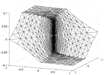
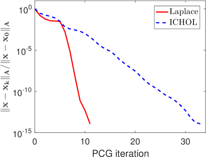
Figure 1: Left: The solution of the problem Eq. 10 on the background of the linear FE triangulation. Right: The relative energy norm of the PCG error as a function of the iteration steps. The Laplace operator preconditioning (solid line) is much more efficient than the incomplete Choleski preconditioning (dashed line), despite the fact that the condition numbers are $161.54$ and close to $16$, respectively. This can be explained by the differences in the associated distribution functions (see the end of Section 4 below).

An example

The following example illustrates in detail the motivation outlined in section 1, i.e. that the condition number may be misleading in characterization of the convergence behavior of the CG method. Consider the boundary value problem

(10) $$-\nabla\cdot(k(x)\nabla u) = 0\quad\text{in}\ \Omega\,,\qquad u=u_{D}\quad\text{on}\ \partial\Omega\,,$$

where the domain $\Omega\equiv(-1,1)\times(-1,1)$ is divided into four subdomains $\Omega_{i}$, $i=1,\,2,\,3,\,4$, corresponding to the axis quadrants numbered counterclockwise. Let $k(x)$ be piecewise constant on the individual subdomains $\Omega_{i}$, $k_{1}=k_{3}\approx 161.45$, $k_{2}=k_{4}=1$. The Dirichlet boundary conditions are described in [28, Section 5.3].

The numerical solution $u$ of this problem and the linear FE discretization, using the standard uniform triangulation, are shown in the left part of Fig. 1. The resulting algebraic problem ${\mathbf{A}}{\mathbf{x}}={\mathbf{b}}$ is solved by the preconditioned conjugate gradient method (PCG). In the right panel of Fig. 1 we see the relative energy norm of the error as a function of iteration steps for the Laplace operator preconditioning (solid line) and for the preconditioning using the algebraic incomplete Choleski factorization of the matrix ${\mathbf{A}}$ (ICHOL) with the drop-off tolerance $10^{-2}$ (dashed line) where the problem has $N=3969$ degrees of freedom. Despite the fact that the spectral condition number $\lambda_{max}/\lambda_{min}$ of the symmetrized preconditioned matrix for the Laplace operator preconditioning is an order of magnitude larger than for the ICHOL preconditioning, close to $161$ and close to $16$, respectively, PCG with the Laplace operator preconditioning clearly demonstrates much faster convergence. This is due to the differences in the distribution of the eigenvalues with the nonnegligible components of the initial residuals in the direction of the associated eigenvectors and effects of rounding errors.

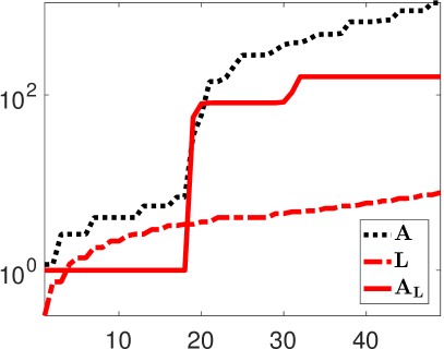
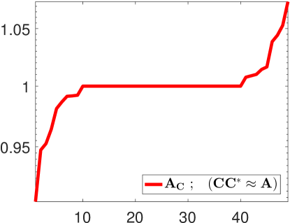
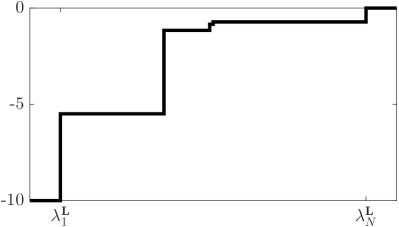
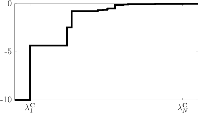
Figure 2: Top: Comparison of the spectra of the matrices ${\mathbf{A}}$, ${\mathbf{A}}_{{\mathbf{L}}}$ and ${\mathbf{A}}_{{\mathbf{C}}}$, $N=49$ degrees of freedom. Due to a small drop-off tolerance, the eigenvalues of ${\mathbf{A}}$ and ${\mathbf{C}}{\mathbf{C}}^{*}$ are graphically indistinguishable. Therefore the right part only shows the eigenvalues of ${\mathbf{A}}_{{\mathbf{C}}}$ (using a different scale than the left part of the figure). Bottom: Comparison of the distribution functions $\omega^{{\mathbf{L}}}(\lambda)$ (left) and $\omega^{{\mathbf{C}}}(\lambda)$ (right) associated with the preconditioned problems. The vertical axes are in the logarithmic scale and $\lambda_{1}^{{\mathbf{L}}}=1$, $\lambda_{N}^{{\mathbf{L}}}=161.45$, $\lambda_{1}^{{\mathbf{C}}}=0.91$, $\lambda_{N}^{{\mathbf{C}}}=1.07$.

The spectra and distribution functions associated with the discretized preconditioned problems are given in Fig. 2 for $N=49$ degrees of freedom and in Fig. 3 for $N=3969$ degrees of freedom. Here, ${\mathbf{L}}={\mathbf{L}}^{1/2}{\mathbf{L}}^{1/2}$ is the matrix associated with the discretized Laplace operator and ${\mathbf{C}}{\mathbf{C}}^{*}\approx{\mathbf{A}}$ is the matrix resulting from ICHOL using the drop-off tolerance $10^{-2}$, with the eigenvalues and eigenvectors of the associated generalized eigenvalue problems (see Eq. 2)

$${\mathbf{A}}{\mathbf{v}}^{{\mathbf{L}}}_{i} =\lambda_{i}^{{\mathbf{L}}}{\mathbf{L}}{\mathbf{v}}^{{\mathbf{L}}}_{i},\quad i=1,\ldots,N,$$

$${\mathbf{A}}{\mathbf{v}}^{{\mathbf{C}}}_{i} =\lambda_{i}^{{\mathbf{C}}}{\mathbf{C}}{\mathbf{C}}^{*}{\mathbf{v}}^{{\mathbf{C}}}_{i},\quad i=1,\ldots,N.$$

The weights of the distribution function $\omega^{{\mathbf{L}}}(\lambda)$, respectively, $\omega^{{\mathbf{C}}}(\lambda)$, associated with the eigenvalues $\lambda_{i}^{{\mathbf{L}}}$, respectively, $\lambda_{i}^{{\mathbf{C}}}$, $i=1\ldots,N$, related to the preconditioned algebraic systems

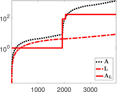
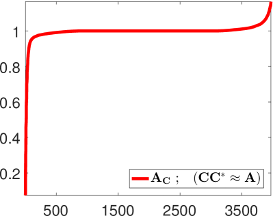
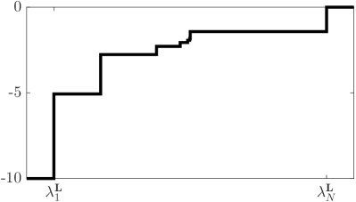
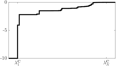
Figure 3: Top: Comparison of the spectra of the matrices ${\mathbf{A}}$, ${\mathbf{A}}_{{\mathbf{L}}}$ and ${\mathbf{A}}_{{\mathbf{C}}}$, $N=3969$ degrees of freedom. Due to a small drop-off tolerance, the eigenvalues of ${\mathbf{A}}$ and ${\mathbf{C}}{\mathbf{C}}^{*}$ are graphically indistinguishable. Therefore the right part only shows the eigenvalues of ${\mathbf{A}}_{{\mathbf{C}}}$ (using a different scale than the left part of the figure). Bottom: Comparison of the distribution functions $\omega^{{\mathbf{L}}}(\lambda)$ (left) and $\omega^{{\mathbf{C}}}(\lambda)$ (right) associated with the preconditioned problems. The vertical axes are in the logarithmic scale and $\lambda_{1}^{{\mathbf{L}}}=1$, $\lambda_{N}^{{\mathbf{L}}}=161.45$, $\lambda_{1}^{{\mathbf{C}}}=7.4\times 10^{-2}$, $\lambda_{N}^{{\mathbf{C}}}=1.16$.

$${\mathbf{A}}_{{\mathbf{L}}}\,({\mathbf{L}}^{1/2}{\mathbf{x}}) ={\mathbf{L}}^{-1/2}{\mathbf{b}},\quad{\mathbf{A}}_{{\mathbf{L}}}={\mathbf{L}}^{-1/2}{\mathbf{A}}{\mathbf{L}}^{-1/2},$$

respectively

$${\mathbf{A}}_{{\mathbf{C}}}\,({\mathbf{C}}^{*}{\mathbf{x}}) ={\mathbf{C}}^{-1}{\mathbf{b}},\quad{\mathbf{A}}_{{\mathbf{C}}}={\mathbf{C}}^{-1}{\mathbf{A}}{\mathbf{C}}^{-*},$$

are given by

(11) $$\omega_{i}^{{\mathbf{L}}}=|(\bar{{\mathbf{v}}}_{i}^{{\mathbf{L}}})^{*}{\mathbf{q}}^{{\mathbf{L}}}|^{2},\quad i=1,\ldots,N,$$

$$\omega_{i}^{{\mathbf{C}}}=|(\bar{{\mathbf{v}}}_{i}^{{\mathbf{C}}})^{*}{\mathbf{q}}^{{\mathbf{C}}}|^{2},\quad i=1,\ldots,N.$$

Here,

$$\bar{{\mathbf{v}}}_{i}^{{\mathbf{L}}}=\frac{{\mathbf{L}}^{1/2}{\mathbf{v}}_{i}^{{\mathbf{L}}}}{\|{\mathbf{L}}^{1/2}{\mathbf{v}}_{i}^{{\mathbf{L}}}\|}\,\quad\mbox{and}\quad\bar{{\mathbf{v}}}_{i}^{{\mathbf{C}}}=\frac{{\mathbf{C}}^{*}{\mathbf{v}}_{i}^{{\mathbf{C}}}}{\|{\mathbf{C}}^{*}{\mathbf{v}}_{i}^{{\mathbf{C}}}\|}\,$$

are the eigenvectors of the Hermitian and positive definite matrix ${\mathbf{A}}_{{\mathbf{L}}}$, respectively, ${\mathbf{A}}_{{\mathbf{C}}}$, and

$${\mathbf{q}}^{{\mathbf{L}}}=\frac{{\mathbf{L}}^{-1/2}{\mathbf{b}}}{\|{\mathbf{L}}^{-1/2}{\mathbf{b}}\|},\quad{\mathbf{q}}^{{\mathbf{C}}}=\frac{{\mathbf{C}}^{-1}{\mathbf{b}}}{\|{\mathbf{C}}^{-1}{\mathbf{b}}\|}.$$

(We use the initial guess ${\mathbf{x}}_{0}=0$). The distribution function $\omega^{{\mathbf{C}}}(\lambda)$ has its points of increase much more evenly distributed in the spectral interval $[\lambda_{1}({\mathbf{A}}_{{\mathbf{C}}}),\lambda_{N}({\mathbf{A}}_{{\mathbf{C}}})]$, which leads to a difference in the PCG convergence behavior. We will return to this issue, and offer a full explanation of the observed CG convergence behavior, after proving the main results and presenting their numerical illustrations.

3 Analysis

As mentioned above, we will not only show that some function values of $k(x)$ are related to the spectrum of ${\mathbf{L}}^{-1}{\mathbf{A}}$, but that there exists a one-to-one correspondence, i.e., a pairing, between the individual eigenvalues of ${\mathbf{L}}^{-1}{\mathbf{A}}$ and quantities given by the function values of $k(x)$ in relation to the supports of the FE basis functions. The proof does not require that $k(x)$ is continuous. If, moreover, $k(x)$ is constant on a part of the domain $\Omega$ that contains fully the supports of one or more basis functions, then the function value of $k(x)$ determines the associated eigenvalue exactly and the number of the involved supports bounds from below the multiplicity of the associated eigenvalue. If $k(x)$ is slowly changing over the support of some basis function, then we get a very accurate localization of the associated eigenvalue.

Our approach is based upon the intervals

(12) $$k({\mathcal{T}}_{j})\equiv[\min_{x\in{\mathcal{T}}_{j}}k(x),\max_{x\in{\mathcal{T}}_{j}}k(x)],\quad j=1,\ldots,N,$$

where ${\mathcal{T}}_{j}=\mbox{supp}(\phi_{j})$. We will first formulate two main results. Theorem 3.1 localizes the positions of all the individual eigenvalues of the matrix ${\mathbf{L}}^{-1}{\mathbf{A}}$ by pairing them with the intervals $k({\mathcal{T}}_{j})$ given in Eq. 12. Using the given pairing, Corollary 3.2 describes the closeness of the eigenvalues to the nodal function values of the scalar function $k(x)$.

The proof of Theorem 3.1 combines perturbation theory for matrices with a classical result from the theory of bipartite graphs. For clarity of exposition, the proof will be presented after stating the corollaries of Theorem 3.1.

Figure 4: Illustration of Theorem 3.1. The diameters of the dashed circles indicate the size of the intervals $k({{\mathcal{T}}_{j}})$, $j=1,\ldots,N$. The dots represent the eigenvalues $\lambda_{j},\ j=1,\ldots,N$, of the matrix ${\mathbf{L}}^{-1}{\mathbf{A}}$. We can find a pairing between the intervals $k({{\mathcal{T}}_{j}})$ and the eigenvalues $\lambda_{i}$, but the pairing may not be uniquely determined.

Theorem 3.1 (Pairing the eigenvalues and the intervals $k({\mathcal{T}}_{j})$, $j=1,\ldots,N$).

Using the previous notation, let $0<\lambda_{1}\leq\lambda_{2}\leq\ldots\leq\lambda_{N}$ be the eigenvalues of , where and are defined by Eqs. 8 and 9 respectively (with the subscript $h$ dropped). As in Eq. 1, let $k(x)$ be measurable and bounded, i.e., $k(x)\in L^{\infty}(\Omega)$. Then there exists a (possibly non-unique) permutation $\pi$ such that the eigenvalues of the matrix satisfy

(13) $$\lambda_{\pi(j)}\in k({{\mathcal{T}}_{j}}),\quad j=1,\ldots,N,$$

where the intervals $k({{\mathcal{T}}_{j}})$ are defined in Eq. 12.

The statement is illustrated in Fig. 4. The proof of the following corollary uses the one-to-one pairing of the intervals Eq. 12, and therefore also the values of $k(x)$ at the nodes of the discretization mesh, with the eigenvalues $\lambda_{\pi(j)}$.

Corollary 3.2 (Pairing the eigenvales and the nodal values).

Using the notation of Theorem 3.1, consider any discretization mesh node $\hat{x}$ such that $\hat{x}\in{{\mathcal{T}}_{j}}$. Then the associated eigenvalue $\lambda_{\pi(j)}$ of the matrix satisfies

(14) $$|\lambda_{\pi(j)}-k(\hat{x})|\leq\max_{x\in{\mathcal{T}}_{j}}|k(x)-k(\hat{x})|.$$

If, in addition, $k(x)\in{\mathcal{C}}^{2}({{\mathcal{T}}_{j}})$, then

$$|\lambda_{\pi(j)}-k(\hat{x})| \leq\max_{x\in{\mathcal{T}}_{j}}|k(x)-k(\hat{x})|$$

(15) $$\leq\hat{h}\|\nabla k(\hat{x})\|+\tfrac{1}{2}\hat{h}^{2}\max_{x\in{\mathcal{T}}_{j}}\|D^{2}k(x)\|$$

where $\hat{h}=\max_{x\in{\mathcal{T}}_{j}}\|x-\hat{x}\|$ and $D^{2}k(x)$ is the second order derivative of the function $k(x)$.

Figure 5: Illustration of Corollary 3.2. The relation Eq. 13 (indicated by the dashed blue circle) can give significantly better localization of the position of the individual eigenvalues than the bounds Eq. 14 (indicated by the dotted red circle) and Eq. 15 (indicated by the solid red circle). When $k(x)$ is constant over ${\mathcal{T}}_{j}$, then $k({\mathcal{T}}_{j})$ reduces to one point $\lambda_{\pi(j)}$; see also Eq. 14. The bound Eq. 15 is weaker that Eqs. 13 and 14, but the evaluation of its first term might be easier in practice.

Proof 3.3.

Since both $\lambda_{\pi(j)}\in k({\mathcal{T}}_{j})$ and $k(\hat{x})\in k({\mathcal{T}}_{j})$, it trivially follows that

$$|\lambda_{\pi(j)}-k(\hat{x})|\leq\max_{x\in{\mathcal{T}}_{j}}|k(x)-k(\hat{x})|.$$

Moreover, for any $x\in{\mathcal{T}}_{j}$, the multidimensional Taylor expansion (see, e.g., [5, p. 11, Section 1.2]) gives for $k(x)\in{\mathcal{C}}^{2}({{\mathcal{T}}_{j}})$ that

$$k(x)-k(\hat{x}) =\nabla k(\hat{x})(x-\hat{x})$$

$$+\tfrac{1}{2}D^{2}k(\hat{x}+\alpha(x-\hat{x}))(x-\hat{x},x-\hat{x})$$

where $\alpha\in[0,1]$, with the absolute value obeying

$$|k(x)-k(\hat{x})| \leq\|\nabla k(\hat{x})\|\|(x-\hat{x})\|$$

$$+\tfrac{1}{2}\|x-\hat{x}\|^{2}\|D^{2}k(\hat{x}+\alpha(x-\hat{x}))\|,$$

giving the statement.

We now give the proof of Theorem 3.1. Lemma 3.4 below and its Corollary 3.6 identify the groups of eigenvalues in any union of intervals

(16) $$\bar{k}({\mathcal{T}}_{{\mathcal{J}}})\equiv\bigcup_{j\in{\mathcal{J}}}k({\mathcal{T}}_{j}),\quad{\mathcal{J}}\subset\{1,\ldots,N\}.$$

This enables us to apply Hall’s theorem, see [4, Theorem 5.2] or, e.g., [16, Theorem 1], to prove Theorem 3.1. (For the sake of completeness, we have also formulated Hall’s result below in Theorem 3.8.)

Lemma 3.4.

Using the notation introduced above, let ${\mathcal{J}}\subset\{1,\ldots,N\}$ and ${\mathcal{T}}_{{\mathcal{J}}}=\cup_{j\in{\mathcal{J}}}{\mathcal{T}}_{j}$. Then there exist at least $p=|{\mathcal{J}}|$ eigenvalues $\tilde{\lambda}_{1},\ldots,\tilde{\lambda}_{p}$ of such that

(17) $$\tilde{\lambda}_{\ell}\in[\min_{x\in{\mathcal{T}}_{\mathcal{J}}}k(x),\max_{x\in{\mathcal{T}}_{\mathcal{J}}}k(x)],\quad\ell=1,\ldots,p.$$

Proof 3.5.

In brief, the proof is based on the theory of eigenvalue perturbations of matrices. We locally modify the scalar function $k(x)$ by setting it equal to a positive constant $K$ in the union ${\mathcal{T}}_{\mathcal{J}}$ of the supports ${\mathcal{T}}_{j}$, $j\in{\mathcal{J}}$. This will result, after discretization, in a modified matrix $\tilde{}_{{\mathcal{J}}}$ such that $K$ is an eigenvalue of of at least $p$ multiplicity. An easy bound for the eigenvalues of

(18)

combined with a standard perturbation theorem for matrices, then provide a bound for the associated $p$ eigenvalues of . A particular choice of the positive constant $K$ will finish the proof.

Let

$$\tilde{k}_{\mathcal{J}}(x) =\begin{cases}K\qquad\mbox{for}\quad x\in{\mathcal{T}}_{{\mathcal{J}}},\\ k(x)\quad\mbox{elsewhere};\end{cases}$$

with

$$\left\langle\tilde{{\mathcal{A}}}_{{\mathcal{J}},h}u,v\right\rangle \equiv\int_{\Omega}\nabla u\cdot\tilde{k}_{\mathcal{J}}\nabla v\,,\quad u,v\in V_{h},$$

where, analogously to Eq. 8,

$$[\tilde{}_{{\mathcal{J}}}]_{lj} =\left\langle\tilde{{\mathcal{A}}}_{{\mathcal{J}},h}\phi_{j},\phi_{l}\right\rangle=\int_{\Omega}\nabla\phi_{l}\cdot\tilde{k}_{{\mathcal{J}}}\nabla\phi_{j}\,.$$

Since $\tilde{k}_{{\mathcal{J}}}$ is constant on each ${\mathcal{T}}_{j},\,j\in{{\mathcal{J}}},$ and the support of the basis function $\phi_{j}$ is ${\mathcal{T}}_{j}$, it holds for any $v\in V_{h}$ that

$$\left\langle\tilde{{\mathcal{A}}}_{{\mathcal{J}},h}\phi_{j},v\right\rangle =\int_{\Omega}\nabla\phi_{j}\cdot\tilde{k}_{{\mathcal{J}}}\nabla v\,=\int_{{\mathcal{T}}_{j}}\nabla\phi_{i}\cdot\tilde{k}_{{\mathcal{J}}}\nabla v\,$$

$$=K\int_{{\mathcal{T}}_{j}}\nabla\phi_{j}\cdot\nabla v\,=K\left\langle{{\mathcal{L}}}_{h}\phi_{j},v\right\rangle,\quad j\in{{\mathcal{J}}}.$$

Thus, $K$ is an eigenvalue of the operator ${\mathcal{L}}_{h}^{-1}\tilde{{\mathcal{A}}}_{{\mathcal{J}},h}$ associated with the eigenfunctions $\phi_{j}$, $j\in{\mathcal{J}}$, and therefore $K$ is the eigenvalue of the matrix with the multiplicity at least $p$. This can also be verified by construction by observing that

$$\tilde{}_{{\mathcal{J}}}$$

Consider now the eigenvalues of ; see Eq. 18. The Rayleigh quotient for an eigenpair $(\theta,$, $\|$, and the associated eigenfunction $q=\sum_{j=1}^{N}\nu_{j}\phi_{j}$, where , satisfies

$$\theta =\frac{\alg{q}^{T}\alg{E}_{{\mathcal{J}}}\alg{q}}{\alg{q}^{T}\alg{L}\alg{q}}=\frac{\alg{q}^{T}(\alg{A}-\tilde{}_{{\mathcal{J}}})\alg{q}}{\alg{q}^{T}\alg{L}\alg{q}}=\frac{\left\langle({\mathcal{A}}_{h}-\tilde{{\mathcal{A}}}_{{\mathcal{J}},h})q,q\right\rangle}{\left\langle{{\mathcal{L}}}_{h}q,q\right\rangle}$$

$$=\frac{\int_{\Omega}\nabla q\cdot(k(x)-\tilde{k}_{{\mathcal{J}}}(x))\nabla q\,dx}{\int_{\Omega}\|\nabla q\|^{2}\,dx}=\frac{\int_{{\mathcal{T}}_{{\mathcal{J}}}}(k(x)-K)\|\nabla q\|^{2}\,dx}{\int_{\Omega}\|\nabla q\|^{2}\,dx},$$

giving

(19) $$|\theta|\leq\max_{x\in{\mathcal{T}}_{{\mathcal{J}}}}|k(x)-K|.$$

Next, consider the symmetric matrices

According to a standard result from the perturbation theory of matrices, see, e.g., [33, Corollary 4.9, p. 203], we find that

$$\lambda_{s}()=\lambda_{s}(\tilde{}+$$

where $\theta_{min}$ and $\theta_{max}$ are the smallest and largest eigenvalues of respectively. Since the matrices , and have the same spectrum as the matrices , and $\tilde{}$, respectively, it follows that

$$\lambda_{s}($$

Due to Eq. 19,

$$\theta_{min} \geq-\max_{x\in{\mathcal{T}}_{{\mathcal{J}}}}|k(x)-K|,$$

$$\theta_{max} \leq\max_{x\in{\mathcal{T}}_{{\mathcal{J}}}}|k(x)-K|,$$

and thus, since $K$ is at least a $p$-multiple eigenvalue of , there exist $p$ eigenvalues $\tilde{\lambda}_{1},\ldots,\tilde{\lambda}_{p}$ of such that

(20) $$\tilde{\lambda}_{\ell}\in[\,K-\max_{x\in{\mathcal{T}}_{{\mathcal{J}}}}|k(x)-K|,\,K+\max_{x\in{\mathcal{T}}_{{\mathcal{J}}}}|k(x)-K|\,],\quad\ell=1,\ldots,p.$$

Setting

$$K=\tfrac{1}{2}(\min_{x\in{\mathcal{T}}_{{\mathcal{J}}}}k(x)+\max_{x\in{\mathcal{T}}_{{\mathcal{J}}}}k(x))$$

gives

$$\tilde{\lambda}_{\ell}\in[\min_{x\in{\mathcal{T}}_{{\mathcal{J}}}}k(x),\max_{x\in{\mathcal{T}}_{{\mathcal{J}}}}k(x)],\quad\ell=1,\ldots,p.$$

Applying Lemma 3.4 $N$ times with ${\mathcal{J}}=\{1\}$, ${\mathcal{J}}=\{2\},\ldots,\,{\mathcal{J}}=\{N\}$, we see that, for the support of any basis function $\phi_{j}$ there is an eigenvalue $\tilde{\lambda}$ of such that $\tilde{\lambda}\in k({{\mathcal{T}}_{j}})$. Moreover, as an additional important consequence, for any subset ${\mathcal{J}}\subset\{1,\ldots,N\}$ the associated union of intervals $\bar{k}({\mathcal{T}}_{{\mathcal{J}}})$ (see Eq. 16) contains at least $p=|{\mathcal{J}}|$ eigenvalues of ; see the following corollary.

Corollary 3.6.

Let, as above, ${\mathcal{J}}\subset\{1,\ldots,N\}$ and ${\mathcal{T}}_{{\mathcal{J}}}=\cup_{j\in{\mathcal{J}}}{\mathcal{T}}_{j}$. Then there exist at least $p=|{\mathcal{J}}|$ eigenvalues $\tilde{\lambda}_{1},\ldots,\tilde{\lambda}_{p}$ of such that

(21) $$\tilde{\lambda}_{\ell}\in\bar{k}({\mathcal{T}}_{{\mathcal{J}}})\equiv\bigcup_{j\in{\mathcal{J}}}k({\mathcal{T}}_{j}),\quad\ell=1,\ldots,p.$$

Moreover, taking ${\mathcal{J}}=\{1,\ldots,N\}$, Eq. 21 immediately implies that any eigenvalue $\tilde{\lambda}$ of belongs to (at least one) interval $k({\mathcal{T}}_{j})$, $j\in\{1,\ldots,N\}$.

Proof 3.7.

Since $\bar{k}({\mathcal{T}}_{j})=k({\mathcal{T}}_{j})$, for any $j\in{\mathcal{J}}$, is an interval Eq. 12, the set $\bar{k}({\mathcal{T}}_{{\mathcal{J}}})$ consists of at most $p$ intervals. We decompose $\bar{k}({\mathcal{T}}_{{\mathcal{J}}})$ into $\tilde{p}$ mutually disjoint intervals, $\tilde{p}\leq p$,

$$\bar{k}({\mathcal{T}}_{{\mathcal{J}}_{i}})\equiv\bigcup_{j\in{\mathcal{J}}_{i}}k({\mathcal{T}}_{j}),\quad i=1,\ldots,\tilde{p}.$$

Lemma 3.4 then assures that each interval $\bar{k}({\mathcal{T}}_{{\mathcal{J}}_{i}})$ contains at least $|{\mathcal{J}}_{i}|$ eigenvalues of . Summing up, at least $\sum_{i=1,\ldots,\tilde{p}}|{\mathcal{J}}_{i}|=|{\mathcal{J}}|$ eigenvalues of must be contained in the union $\bar{k}({\mathcal{T}}_{{\mathcal{J}}})$.

In order to finalize the proof of Theorem 3.1, we still need to show the existence of a one-to-one pairing between the individual eigenvalues and the individual intervals $k({\mathcal{T}}_{j}),\ j=1,\ldots,N$. The relationship between the intervals $k({\mathcal{T}}_{j})$, $j=1,\ldots,N$, and the eigenvalues of described in Lemma 3.4 and Corollary 3.6 can be represented by the following bipartite graph. Let, as above, $0<\lambda_{1}\leq\lambda_{2}\leq\ldots\leq\lambda_{N}$ be the eigenvalues of . Consider the bipartite graph

(22) $$({\mathcal{S}},{\mathcal{I}},E)$$

with the sets of nodes ${\mathcal{S}}={\mathcal{I}}=\{1,\ldots,N\}$ and the set of edges $E$, where

$$\{s,i\}\in E\quad\mbox{if and only if}\quad\lambda_{s}\in k({\mathcal{T}}_{i}),\quad s\in{\mathcal{S}},\ i\in{\mathcal{I}}.$$

A subset of edges $M\subset E$ is called matching if no edges from $M$ share a common node; see [4, Section 5.1]. We will use the following famous theorem.

Theorem 3.8 (Hall’s theorem).

Let $({\mathcal{S}},{\mathcal{I}},E)$ be a bipartite graph. Given ${\mathcal{J}}\subset{\mathcal{I}}$, let $G({\mathcal{J}})\subset{\mathcal{S}}$ denote the set of all nodes adjacent to any node from ${\mathcal{J}}$, i.e.,

$$G({\mathcal{J}})=\{s\in{\mathcal{S}};\ \exists i\in{\mathcal{J}}\mbox{ such that }\{s,i\}\in E\}.$$

Then there exists a matching $M\subset E$ that covers ${\mathcal{I}}$ if and only if

(23) $$|G({\mathcal{J}})|\geq|{\mathcal{J}}|\quad\mbox{for any}\quad{\mathcal{J}}\subset{\mathcal{I}};$$

see, e.g., [4, Theorem 5.2] and the original formulation [16, Theorem 1].

Now we are ready to finalize our argument.

Proof of Theorem 3.1

Consider the bipartite graph defined by Eq. 22 and let $G({\mathcal{J}})\subset{\mathcal{S}}$ be the set of all nodes (representing the eigenvalues) adjacent to any node from ${\mathcal{J}}$, ${\mathcal{J}}\subset{\mathcal{I}}$ (representing the intervals). In other words, $G({\mathcal{J}})$ represents the indices of all eigenvalues $\{\lambda_{s};\ s\in G({\mathcal{J}})\}$ located in $\bar{k}({\mathcal{T}}_{{\mathcal{J}}})=\cup_{j\in{\mathcal{J}}}k({\mathcal{T}}_{j})$. Corollary 3.6 of Lemma 3.4 assures that assumption Eq. 23 in Theorem 3.8 is satisfied, i.e.

(24) $$|G({\mathcal{J}})|\geq|{\mathcal{J}}|.$$

Thus, according to Theorem 3.8, there exist a matching $M\subset E$ that covers ${\mathcal{I}}$. Since $|{\mathcal{I}}|=|{\mathcal{S}}|$, this matching defines the permutation $\pi(i),\ i=1,2,\ldots,N$, such that

$$\lambda_{\pi(i)}\in k({\mathcal{T}}_{i}),\quad i=1,\ldots,N,$$

which finishes the proof.

4 Numerical experiments

In this section we will illustrate the theoretical results by a series of numerical experiments. We will investigate how well the nodal values of $k$ correspond to the eigenvalues and assess the sharpness of the estimates in Corollary 3.2 in a few examples, including both uniform and local mesh refinement. Furthermore, we will compute the corresponding intervals $k({\mathcal{T}}_{j}),\ j=1,\ldots,N$ and consider the pairing in Theorem 3.1.

Test problems

We will consider four test problems defined on the domain $\Omega\equiv(0,1)\times(0,1)$ where we slightly abuse the notation above and let $k=k(x,y)$. The first three problems use a continuous coefficient function $k(x,y)$:

(P1) $$k(x,y) =\sin(x+y),$$

(P2) $$k(x,y) =1+50\exp(-5(x^{2}+y^{2})),$$

(P3) $$k(x,y) =2^{7}(x^{7}+y^{7}).$$

The fourth problem uses a discontinuous function $k(x,y)$,

$$\mbox{(P4)}\quad k(x,y)\ = \begin{cases}\mbox{(P1)}\quad\mbox{for}\ (x,y)\in(0,1)\times(\tfrac{1}{2},1),\\ \mbox{(P2)}\quad\mbox{elsewhere}.\end{cases}$$

Numerical experiments were computed using FEniCS [23] and Matlab. If not specified otherwise, we consider a triangular uniform mesh with piecewise linear discretization basis functions.

4.1 Illustration of Theorem 3.1 and Corollary 3.2

In Fig. 6 we show the nodal values of $k(x,y)$ and the corresponding eigenvalues, both sorted in increasing order on the unit square with $N=81$ degrees of freedom. Clearly, there is a close correspondence between the nodal values and the eigenvalues even at this relatively coarse resolution, but there are some notable differences for (P3) and (P4) that are clearly visible.

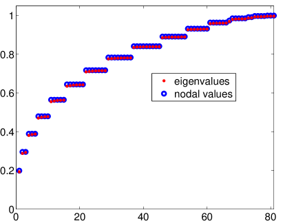
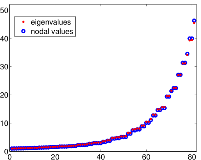
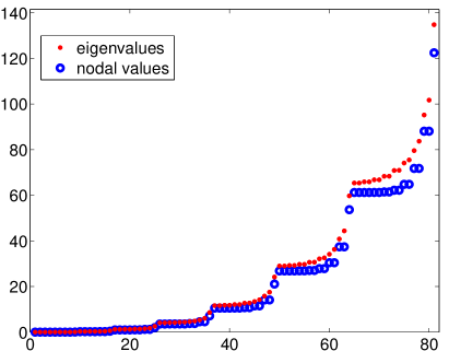
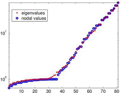
Figure 6: Comparison of the eigenvalues $\lambda_{s}$, $s=1,\ldots,N$ (red dots) and the increasingly sorted nodal values of $k$ (blue circles). Top left: (P1), top right: (P2), bottom left: (P3), bottom right: (P4). As in Fig. 7, we use the semilogarithmic scale in the lower right panel (P4).

Theorem 3.1 states that there exists a pairing $\pi$ such that $\lambda_{\pi(i)}\in k({\mathcal{T}}_{i})$ for every $i=1,\ldots,N$. The proof is not constructive and it is therefore interesting to consider potential pairings. In Fig. 7 we show the results of the previously mentioned paring of the eigenvalues and the intervals $k({\mathcal{T}}_{i})~{}=~{}k({\mathcal{T}(x_{i},y_{i})})$ where the vertices $(x_{i},y_{i})$ have been sorted such that the nodal values $k(x_{i},y_{i})$ are in increasing order. The pairing appears to work quite well except for the case (P4) where in particular the eigenvalues between 30-40 are outside the intervals provided by this pairing.

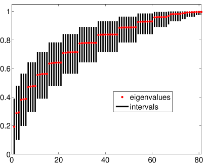
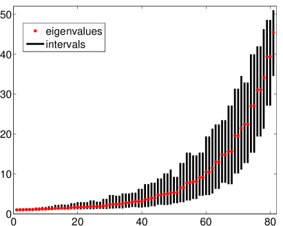
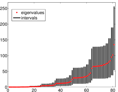
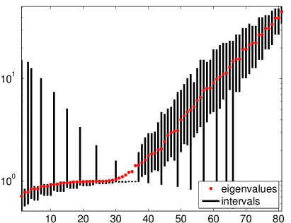
Figure 7: The eigenvalues $\lambda_{1}\leq\ldots\leq\lambda_{N}$ (red dots) and the associated intervals $k({\mathcal{T}}_{P(s)})$ (black vertical lines), where the pairing $P$ is defined by the increasingly sorted nodal values of $k$; see Fig. 6. Top left: (P1), top right: (P2), bottom left: (P3), bottom right: (P4). We observe that for (P4) some of the eigenvalues are not inside the associated intervals and therefore the ordering in which eigenvalues and nodal values of $k$ are in increasing order does not in this case conform to $\pi$ from Theorem 3.1.

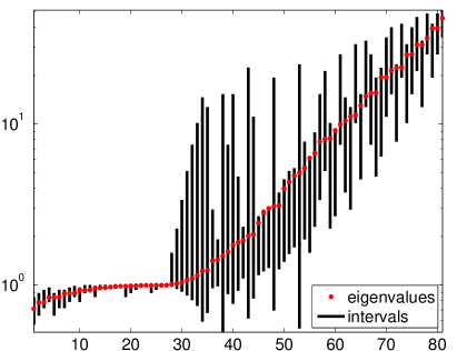
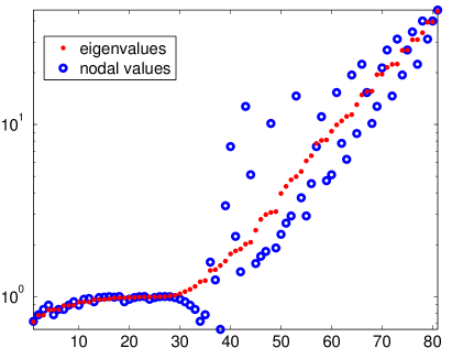
Figure 8: Illustration of the pairing $\pi$ computed by the Dulmage-Mendelsohn decomposition of the corresponding adjacency matrix (see LABEL:eq:G) for problem (P4). Left: The eigenvalues $\lambda_{1}\leq\ldots\leq\lambda_{N}$ (red dots) and the associated intervals $k({\mathcal{T}}_{\pi^{-1}(s)})$ (black vertical lines). Right: The comparison of the eigenvalues and the associated nodal values $k_{\pi^{-1}(s)}$ (blue circles).

In order to ensure that we employ a proper pairing, i.e., to guarantee that $\lambda_{\pi(i)}\in k({\mathcal{T}}_{i})$, $i=1,\ldots,N$, we construct the adjacency matrix such that

(25)

By using the Dulmage-Mendelsohn decomposition of this adjacency matrix (provided by the Matlab command dmperm) we get a pairing $\pi$ satisfying $\lambda_{\pi(i)}\in k({\mathcal{T}}_{i})$ for every $i=1,\ldots,N$. Figure 8 illustrates the pairing $\pi$ from Theorem 3.1 for (P4) and the approximation of the eigenvalues by the associated nodal values (the plots in Fig. 8 should be compared with the lower right panels of Figs. 6 and 7).

The difference between the nodal values and the corresponding eigenvalues is estimated in Eq. 15 and to assess the sharpness of this estimate, Fig. 9 compares the quantities $|\lambda_{s}-k_{\pi^{-1}(s)}|$ (red dots) with the first term on the right hand side of Eq. 15 (black stars). We observe that the first term of Eq. 15 in general overestimate the differences at this coarse resolution.

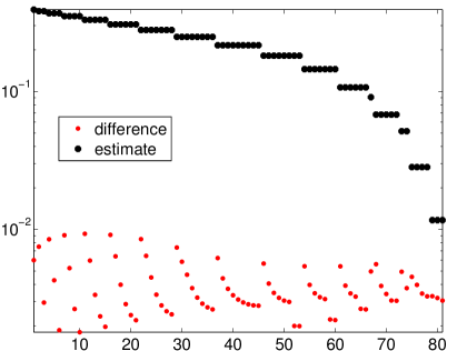
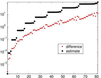
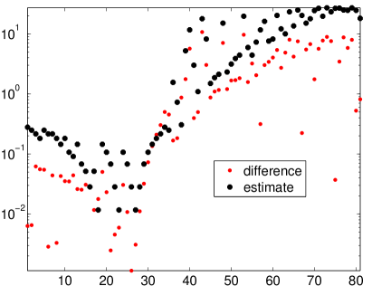
Figure 9: Illustration of Corollary 3.2. Comparison of the absolute difference $|\lambda_{s}-k_{\pi^{-1}(s)}|$ (red dots) and its estimate by the first term on the right hand side of Eq. 15 (black stars). Top left: (P1), top right: (P2), bottom left: (P3), bottom right: (P4).

4.2 Effects of $h$-adaptivity

Corollary 3.2 states that the estimated difference $|\lambda_{s}~{}-~{}k_{\pi^{-1}(s)}|$ improves at least linearly as the mesh is refined. Figure 10 shows the improvement of both the nodal value estimates of $k$ and the associated intervals $k({\mathcal{T}}_{\pi^{-1}(s)})$ for problems (P1) and (P3) with $N=59^{2}=3481$ degrees of freedom. (We would also like to note that the proof of Corollary 3.2 does not assume linear Lagrange elements, but holds for any type of nodal basis functions.)

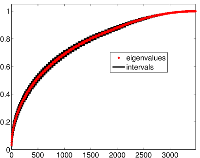
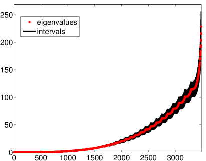
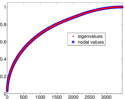
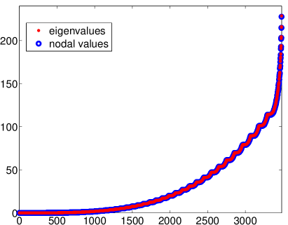
Figure 10: Top: The eigenvalues $\lambda_{s}$, $s=1,\ldots,N$ (red dots) and the associated intervals $k({\mathcal{T}}_{\pi^{-1}(s)})$ (black vertical lines). Bottom: Comparison of the eigenvalues $\lambda_{s}$ and the nodal values $k_{\pi^{-1}(s)}$ (blue circles). Here we use uniform mesh with $N=3481$ degrees of freedom. Left: (P1), right: (P3). We can observe a dramatic improvement of the approximation accuracy, cf. Figs. 6 and 7.

Corollary 3.2 is a local estimate which allows local mesh refinement for improving accuracy of the eigenvalue estimate. To see the effect of locally refined mesh on the spectrum of the preconditioned problem, we consider the test problem (P2), where we refine the mesh in the subdomain $[0,0.2]\times[0,0.2]$, i.e., in the area with large gradient of the function $k(x,y)$. Figure 11 shows the discretization mesh (top), the eigenvalues with the associated intervals (middle) and the associated nodal values (bottom). As expected, we observe more eigenvalues in the upper part of the spectrum as well as their better localization; see for comparison also the top right panels of Figs. 6 and 7.

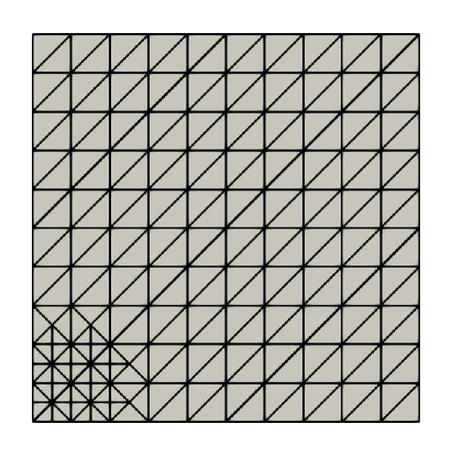
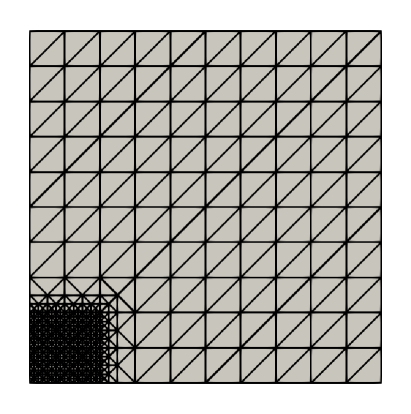
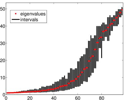
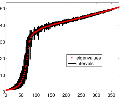
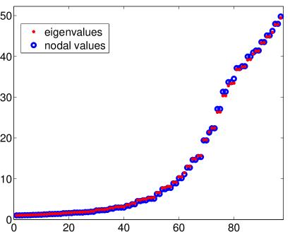
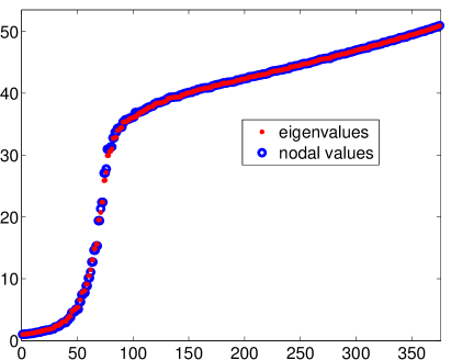
Figure 11: The influence of the locally refined mesh in the subdomain $(0,0.2)\times(0,0.2)$ for the test problem (P2). Left: One refinement step. Right: Three refinement steps. We use the same symbols as in Figs. 6 and 7.

4.3 Re-entrant corner domain

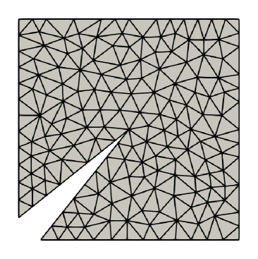
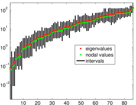
Figure 12: Comparison of the eigenvalues $\lambda_{s}$ (red dots) with the sorted nodal values $k_{\pi^{-1}(s)}$ (green circles) and the associated intervals $k({\mathcal{T}}_{\pi^{-1}(s)})$ (black vertical lines) for the test problem (P3) on the re-entrant corner domain.

The local considerations of Corollary 3.2 does not require additional regularity for the solutions of the associated PDEs and our theoretical results are valid for domains of any shape. To illuminate that no additional regularity is needed we conduct experiments on a domain with a re-entrant corner, i.e.,

$$\Omega =[0,1]\times[0,1]\setminus\left\{(x,y):x>0.8y+0.1\quad\&\quad y<0.8x+0.1\right\}.$$

The domain is shown in the left panel in Fig. 12, while the eigenvalues $\lambda_{s}$ (red dots) with the sorted nodal values $k_{\pi^{-1}(s)}$ (green circles) and the associated intervals $k({\mathcal{T}}_{\pi^{-1}(s)})$ (black vertical lines) for test problem (P3) are shown in the right panel.

4.4 Convergence of the introductory example explained

We will now finish our exposition by returning back to the motivation example presented in Section 2 and by explaining the difference in the behavior of PCG with the Laplace operator preconditioning and with the ICHOL preconditioning; see the right part of Fig. 1.

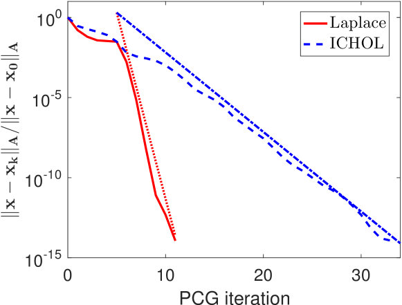
Figure 13: Explanation of the PCG behavior from Figure 1. The dotted and dash-dotted lines show the estimates of the PCG error based on the so-called effective condition number, which here (see the discussion in the text) fully describes the PCG behavior starting from the sixth iteration.

First we present Fig. 13, a modification of Fig. 1, showing that at the fifth iteration we can identify with a remarkable accuracy the slope of the PCG convergence curves for most of the subsequent iterations, with the convergence being almost linear without a substantial acceleration. The rate of convergence is for the Laplace operator preconditioning remarkably faster than for the ICHOL preconditioning.

Table 1: Detail of the points of increase (Ritz values) and the weights (see Eq. 11) of the distribution function $\omega(\lambda)$ associated with the problem preconditioned by the Laplace operator. The effective condition number is for the given example determined by $\lambda_{1926}$ and $\lambda_{2039}$; see the top part of Fig. 15.

Index	1 – 1922	1923	1924	1925	1926
Eigenvalues	$1$	$28.508$	$61.384$	$75.324$	$\lambda_{1926}=79.699$
Total weight	$9\times 10^{-6}$	$\approx 10^{-3}$	$\approx 10^{-3}$	$\approx 10^{-3}$	$\approx 10^{-3}$
Index	1927 – 1930	1931 – 2039	2040 – 2047		2048 – 3969
Eigenvalues	$80.875$ – $81.222$	$\lambda_{2039}=81.224$	$81.226$ – $133.94$		$161.45$
Total weight	$\approx 10^{-3}$	$1.8\times 10^{-2}$	$8\times 10^{-10}$		$0.96$

The convergence of the PCG method with the Laplace operator preconditioning can be completely explained using Theorem 3.1 and the results about the CG convergence behavior from the literature. Since $k(x)$ is in the given experiment constant for most of the supports of the basis functions (being equal to one respectively to $161.45$), according to Theorem 3.1 the preconditioned system matrix must have many multiple eigenvalues equal to one respectively to $161.45$. This is illustrated by the computed quantities presented in Table 1. We see that $1922$ eigenvalues are equal to one, $1922$ are equal to $161.45$ and the rest is spread between $\approx 28$ and $\approx 134$ (with the eigenvalues between $81.226$ and $134$ of so negligible weight (see Eq. 11) that they do not contribute within the small number of iterations to the computations; they are for CG computations within the given number of iterations practically not visible; see [22, Section 5.6.4]).

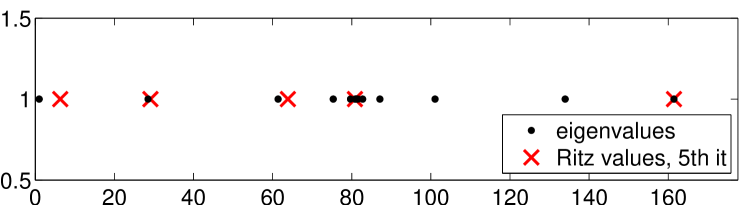
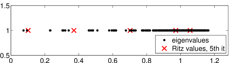
Figure 14: Illustration of the Ritz values computed at the fifth PCG iteration. Top: Problem with the Laplace operator preconditioning. We observe four Ritz values approximating the eigenvalues at the lower end of the spectrum and one Ritz value very closely approximating the largest eigenvalue. Bottom: Problem with the ICHOL preconditioning. We do not observe yet a good approximation of any of the eigenvalues, but we can see that the extremal Ritz values approach the ends of the spectral interval.

Assuming exact arithmetic, van der Sluis and van der Vorst prove in the seminal paper [35] that, if the Ritz values approximate (in a rather moderate way) the eigenvalues at the lower end of the spectrum, the computations further proceed with a rate as if the approximated eigenvalues are not present. Analysis of rounding errors in CG and Lanczos by Paige, Greenbaum and others, mentioned above in Section 1, then proves that this argumentation concerning the lower end of the spectrum remains valid also in finite precision arithmetic computations. At the fifth iteration the eigenvalues $1$, $28.5$, $61.4$, $75.3$ at the lower end of the spectrum and also the largest eigenvalue $161.45$ are approximated by the Ritz values; see Fig. 14. Therefore, from then on PCG converges, using the effective condition number upper bound

(26) $$\frac{\|\alg{x}-\alg{x}_{k}\|}{\|\alg{x}-\alg{x}_{0}\|}\leq 2\left(\frac{\sqrt{\kappa_{e}}-1}{\sqrt{\kappa_{e}}+1}\right)^{k-5},\ \kappa_{e}=\frac{\lambda_{2039}}{\lambda_{1926}}=1.02,\quad k>5,$$

at least as fast as the right hand side in Eq. 26 suggests. The convergence is in the iterations $6$–$9$ very fast and therefore we do not practically observe any further acceleration. At iteration $10$, the convergence slows down. This is due to the effect of rounding errors that cause forming a second Ritz value that approximates the largest eigenvalue $161.45$ (as mentioned above, the appearance of large outlying eigenvalues can cause deterioration of convergence due to roundoff; the detailed explanation is given, e.g., in [12], [22, Section 5.9.1; see in particular, Figures 5.14 and 5.15] and in [9]).

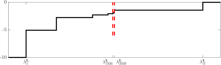
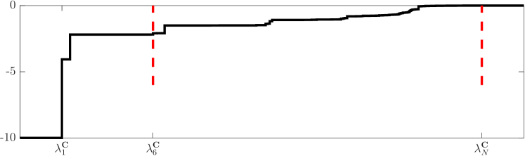
Figure 15: Distribution functions: Top: Laplace operator preconditioning. Bottom: ICHOL preconditioning. Red dashed lines represent the position of eigenvalues associated with the effective condition numbers after five iterations.

Table 2: Detail of the points of increase (Ritz values) and the weights (see Eq. 11) of the distribution function $\omega(\lambda)$ associated with the problem with ICHOL preconditioning. The effective condition number is for the given example determined by $\lambda_{6}$ and $\lambda_{3969}$; see the bottom part of Fig. 15.

Index	1	2	3	4
Eigenvalues	$0.074$	$0.095$	$0.231$	$0.233$
Total weight	$8\times 10^{-5}$	$6.4\times 10^{-3}$	$8\times 10^{-7}$	$10^{-8}$
Index	5	6	7 – 3969
Eigenvalues	$0.304$	$\lambda_{6}=0.311$	$0.321$ – $\lambda_{3969}=1.1643$
Total weight	$6\times 10^{-5}$	$1.5\times 10^{-3}$	$0.992$

Also for the incomplete Choleski preconditioning an analogous argumentation holds with the difference that the approximation of the five leftmost eigenvalues by the Ritz values slightly accelerate convergence. The bound Eq. 26 is valid with replacing $\kappa_{e}$ by

$$\kappa_{e}=\frac{\lambda_{3969}}{\lambda_{6}}=3.75;$$

see the computed quantities in Table 2. We can see from Fig. 14 that at the fifth iteration the five smallest eigenvalues are not yet approximated by the Ritz values. This needs about five additional iterations. From the tenth iteration the convergence remains very close to linear and slow because no further acceleration can take place due to the widespread eigenvalues and the effects of roundoff (no further eigenvalue approximation can significantly affect the convergence behavior). The part of the spectra that practically determine the convergence rates after the fifth iteration of the Laplace operator PCG, respectively, after the tenth iteration of the ICHOL PCG are illustrated in Fig. 15.

5 Concluding remarks

We have analyzed the operator $\mathcal{L}^{-1}\mathcal{A}$ generated by preconditioning second order elliptic PDEs with the inverse of the Laplacian. Previously, it has been proven that the range of the coefficient function $k$ of the elliptic PDE is contained in the spectrum of $\mathcal{L}^{-1}\mathcal{A}$, but only for operators defined on infinitely dimensional spaces. In this paper we show that a substantially stronger result holds in the discrete case of conforming finite elements. More precisely, that the eigenvalues of the matrix , where and are FE-matrices, lie in resolution dependent intervals around the nodal values of the coefficient function that tend to the nodal values as the resolution increases. Moreover, there is a pairing (possibly non-unique) of the eigenvalues and the nodal values of the coefficient function due to Hall’s theory of bipartite graphs. Finally, we demonstrate that the conjugate gradient method utilize the structure of the spectrum (more precisely, of the associated distribution function) to accelerate the iterations. In fact, even though the condition number involved, for instance, with incomplete Choleski preconditioning is significantly smaller than for the Laplacian preconditioner, the performance when using Choleski is much worse. In this case, the accelerated performance of the Laplacian preconditioner can be fully explained by an analysis of the distribution functions.

References

- [1] O. Axelsson, Iterative Solution Methods, Cambridge University Press, 1994, https://doi.org/10.1017/cbo9780511624100.
- [2] O. Axelsson and G. Lindskog, On the eigenvalue distribution of a class of preconditioning methods, Numer. Math., (1986), pp. 479–498, https://doi.org/10.1007/bf01389447.
- [3] O. Axelsson and G. Lindskog, On the rate of convergence of the preconditioned conjugate gradient method, Numer. Math., (1986), pp. 499–523, https://doi.org/10.1007/bf01389448.
- [4] J. A. Bondy and U. S. R. Murty, Graph theory with applications, American Elsevier Publishing Co., Inc., New York, 1976, https://doi.org/10.1007/978-1-349-03521-2.
- [5] P. G. Ciarlet, The finite element method for elliptic problems, vol. 40 of Classics in Applied Mathematics, Society for Industrial and Applied Mathematics (SIAM), Philadelphia, PA, 2002, https://doi.org/10.1137/1.9780898719208. Reprint of the 1978 original [North-Holland, Amsterdam; MR0520174 (58 #25001)].
- [6] A. L. Dulmage and N. S. Mendelsohn, Coverings of bipartite graphs, Canad. J. Math., 10 (1958), pp. 517–534, https://doi.org/10.4153/CJM-1958-052-0.
- [7] M. Engeli, T. Ginsburg, H. Rutishauser, and E. Stiefel, Refined iterative methods for computation of the solution and the eigenvalues of self-adjoint boundary value problems, Mitt. Inst. Angew. Math. Zürich, 8 (1959), p. 107, https://doi.org/10.1007/978-3-0348-7224-9.
- [8] V. Faber, T. A. Manteuffel, and S. V. Parter, On the theory of equivalent operators and application to the numerical solution of uniformly elliptic partial differential equations, Adv. in Appl. Math., 11 (1990), pp. 109–163, https://doi.org/10.1016/0196-8858(90)90007-L.
- [9] T. Gergelits and Z. Strakoš, Composite convergence bounds based on Chebyshev polynomials and finite precision conjugate gradient computations, Numerical Algorithms, 65 (2014), pp. 759–782, https://doi.org/10.1007/s11075-013-9713-z.
- [10] A. Greenbaum, Behavior of slightly perturbed Lanczos and conjugate-gradient recurrences, Linear Algebra Appl., 113 (1989), pp. 7–63, https://doi.org/10.1016/0024-3795(89)90285-1.
- [11] A. Greenbaum, V. Pták, and Z. Strakoš, Any nonincreasing convergence curve is possible for GMRES, SIAM J. Matrix Anal. Appl., 17 (1996), pp. 465–469, https://doi.org/10.1137/s0895479894275030.
- [12] A. Greenbaum and Z. Strakoš, Predicting the behavior of finite precision Lanczos and conjugate gradient computations, SIAM J. Matrix Anal. Appl., 13 (1992), pp. 121–137, https://doi.org/10.1137/0613011.
- [13] A. Greenbaum and Z. Strakoš, Matrices that generate the same Krylov residual spaces, in Recent advances in iterative methods, vol. 60 of IMA Vol. Math. Appl., Springer, New York, 1994, pp. 95–118, https://doi.org/10.1007/978-1-4613-9353-5_7.
- [14] A. Günnel, R. Herzog, and E. Sachs, A note on preconditioners and scalar products in Krylov subspace methods for self-adjoint problems in Hilbert space, Electronic Transactions on Numerical Analysis, 41 (2014), pp. 13–20, http://elibm.org/article/10006339.
- [15] W. Hackbusch, Iterative solution of large sparse systems of equations, Springer-Verlag, 1994, https://doi.org/10.1007/978-3-319-28483-5.
- [16] P. Hall, On representatives of subsets, Journal of the London Mathematical Society, s1-10 (1935), pp. 26–30, https://doi.org/10.1112/jlms/s1-10.37.26, https://arxiv.org/abs/https://londmathsoc.onlinelibrary.wiley.com/doi/pdf/10.1112/jlms/s1-10.37.26.
- [17] M. R. Hestenes and E. Stiefel, Methods of conjugate gradients for solving linear systems, J. Research Nat. Bur. Standards, 49 (1952), pp. 409–436, https://doi.org/10.6028/jres.049.044.
- [18] R. Hiptmair, Operator preconditioning, Computers & Mathematics with Applications. An International Journal, 52 (2006), pp. 699–706, https://doi.org/10.1016/j.camwa.2006.10.008.
- [19] A. Jennings, Influence of the eigenvalue spectrum on the convergence rate of the conjugate gradient method, J. Inst. Math. Appl., 20 (1977), pp. 61–72, https://doi.org/10.1093/imamat/20.1.61.
- [20] A. Jennings and G. M. Malik, The solution of sparse linear equations by the conjugate gradient method, Internat. J. Numer. Methods Engrg., 12 (1978), pp. 141–158, https://doi.org/10.1002/nme.1620120114.
- [21] C. Lanczos, Solution of systems of linear equations by minimized iterations, J. Research Nat. Bur. Standards, 49 (1952), pp. 33–53, https://doi.org/10.6028/jres.049.006.
- [22] J. Liesen and Z. Strakoš, Krylov subspace methods: principles and analysis, Numerical Mathematics and Scientific Computation, Oxford University Press, Oxford, 2012, https://doi.org/10.1093/acprof:oso/9780199655410.001.0001. Principles and analysis.
- [23] A. Logg, K.-A. Mardal, G. N. Wells, et al., Automated Solution of Differential Equations by the Finite Element Method, Springer, 2012, https://doi.org/10.1007/978-3-642-23099-8.
- [24] J. Málek and Z. Strakoš, Preconditioning and the conjugate gradient method in the context of solving pdes, SIAM Spotlight Series, Dec. 2014, https://doi.org/10.1137/1.9781611973846.
- [25] K. A. Mardal and R. Winther, Preconditioning discretizations of systems of partial differential equations, Numerical Linear Algebra with Applications, 18 (2011), pp. 1–40.
- [26] G. Meurant, The Lanczos and Conjugate Gradient Algorithms. From Theory to Finite Precision Computations, vol. 19 of Software, Environments, and Tools, Society for Industrial and Applied Mathematics (SIAM), Philadelphia, PA, 2006, https://doi.org/10.1137/1.9780898718140.
- [27] G. Meurant and Z. Strakoš, The Lanczos and conjugate gradient algorithms in finite precision arithmetic, Acta Numer., 15 (2006), pp. 471–542, https://doi.org/10.1017/S096249290626001X.
- [28] P. Morin, R. H. Nochetto, and K. G. Siebert, Convergence of adaptive finite element methods, SIAM Review, 44 (2002), pp. 631–658, https://doi.org/10.1137/S0036144502409093.
- [29] B. F. Nielsen and K. A. Mardal, Analysis of the minimal residual method applied to ill-posed optimality systems, SIAM Journal on Scientific Computing, 35 (2013), pp. A785–A814, https://doi.org/10.1137/120871547.
- [30] B. F. Nielsen, A. Tveito, and W. Hackbusch, Preconditioning by inverting the Laplacian; an analysis of the eigenvalues, IMA Journal of Numerical Analysis, 29 (2009), pp. 24–42.
- [31] C. C. Paige, The Computation of Eigenvalues and Eigenvectors of Very Large and Sparse Matrices, PhD thesis, London University, London, England, 1971.
- [32] C. C. Paige, Accuracy and effectiveness of the Lanczos algorithm for the symmetric eigenproblem, Linear Algebra Appl., 34 (1980), pp. 235–258, https://doi.org/10.1016/0024-3795(80)90167-6.
- [33] G. W. Stewart and J. G. Sun, Matrix perturbation theory, Computer Science and Scientific Computing, Academic Press, Inc., Boston, MA, 1990.
- [34] Z. Strakoš, On the real convergence rate of the conjugate gradient method, Linear Algebra Appl., 154/156 (1991), pp. 535–549, https://doi.org/10.1016/0024-3795(91)90393-B.
- [35] A. van der Sluis and H. A. van der Vorst, The rate of convergence of conjugate gradients, Numer. Math., 48 (1986), pp. 543–560, https://doi.org/10.1007/BF01389450.
- [36] J. von Neumann, Mathematical foundations of quantum mechanics, Princeton Landmarks in Mathematics, Princeton University Press, Princeton, NJ, 1996, https://doi.org/10.2307/j.ctt1wq8zhp. Translated from the German print published in 1932 and with a preface by Robert T. Beyer, Twelfth printing, Princeton Paperbacks.
- [37] Y. V. Vorobyev, Methods of Moments in Applied Mathematics, Translated from the Russian by Bernard Seckler, Gordon and Breach Science Publishers, New York, 1965, https://doi.org/10.2307/2004791.