Scaling behavior in interacting systems: joint effect of anisotropy and compressibility

Abstract

Motivated by the ubiquity of turbulent flows in realistic conditions, effects of turbulent advection on two models of classical non-linear systems are investigated. In particular, we analyze model A (according to the Hohenberg-Halperin classification hohenberg ) of a non-conserved order parameter and a model of the direct bond percolation process. Having two paradigmatic representatives of distinct stochastic dynamics, our aim is to elucidate to what extent velocity fluctuations affect their scaling behavior. The main emphasis is put on an interplay between anisotropy and compressibility of the velocity flow on their respective scaling regimes. Velocity fluctuations are generated by means of the Kraichnan rapid-change model, in which the anisotropy is due to a distinguished spatial direction $\bm{n}$ and a correlator of the velocity field obeys the Gaussian distribution law with prescribed statistical properties. As the main theoretical tool, the field-theoretic perturbative renormalization group is adopted. Actual calculations are performed in the leading (one-loop) approximation. Having obtained infra-red stable asymptotic regimes, we have found four possible candidates for macroscopically observable behavior for each model. In contrast to the isotropic case, anisotropy brings about enhancement of non-linearities and non-trivial regimes are proved to be more stable.

1 Introduction

Critical behavior is present in many important physical phenomena. A genuine interest in critical fluids stems from a fact that it represents a typical non-linear problem and as such proves to be a challenging and enriching problem both from a theoretical and an experimental point of view. The main research focus is devoted to an analysis of specific physical, thermodynamic and transport properties. Majority of studies in the past employed a model of a pure fluid without any additional interactions. However, later it became clear that hydrodynamic effects cannot be ignored due to a strong sensitivity of such systems to external disturbances ivanov ; sep . These effects come into play via coupling between a critical fluid and an external environment in which fluid motion sets in. A substantial increase of compressibility, which is given by the derivative $\left(\partial\rho/\partial p\right)_{T}$ (where $\rho$ is the density of a fluid, $p$ is the pressure, and $T$ is the temperature in system), brings about so-called stratification effect: as density grows under the fluid’s own weight, a distinguished direction $\bm{n}$ in the medium emerges Anisimov ; comp1 ; comp3 . Naturally, vector $\bm{n}$ is parallel to the vector of gravity force $\bm{g}$ and also to the density gradient, i.e. $\bm{n}\,||\,\bm{\nabla}\rho$.

The environment can have an additional effect and may affect behavior profoundly Jan97 . In addition to external forces, such as gravitational, magnetic or electric field, there is another conceivable mechanism leading to a non-equilibrium state: turbulence caused by shaking, stirring, and flow generation that is abundantly observed in many natural phenomena davidson ; frisch ; monin . From a general standpoint, turbulence is a rule rather than exception davidson and in order to have a complete physical picture turbulence should be incorporated in a theoretical description.

Critical phenomena in chaotically stirred mediums are abundant in nature as well. Of particular interest are fluids in turbulent motion, which manifest universal behavior known as the Kolmogorov scaling in the case of fully developed turbulence davidson ; frisch ; monin . The effect of stirring by a fully developed turbulent flow has been investigated in numerous papers, see for instance frisch ; monin ; FGV01 ; turbo ; HHL16 and references therein. Research activity regarding turbulence is enormous, but still many important problems remain unsolved. In theoretical physics there are two accepted approaches that allow us to include turbulence into consideration: the synthetic velocity ensemble and the stochastic Navier-Stokes equation. A typical example of the former is embodied in the rapid-change Kraichnan model and its descendants FGV01 ; kr1 ; kr2 ; kr3 ; kr4 . An underlying idea is to generate the velocity field ${\bm{v}}(\bm{x},t)$ by means of a statistical ensemble with prescribed properties, which are chosen in a suitable way FGV01 ; turbo . Usually one assumes the Gaussian distribution law with zero mean and a correlation function in the form $\propto\delta(t-t^{\prime})|\bm{x}-\bm{x}^{\prime}|^{\delta}$. The latter (microscopic) approach to a description of velocity field has its own dynamics governed by the Navier-Stokes equation turbo ; nav1 ; jurcisin2 augmented with a proper stochastic term, which mimics an input of energy into a system. This approach is motivated by a fluctuation theory of critical phenomena nav1 ; pata . Though this approach is more satisfying from the physical point of view, in this work we consider a specific modification of the Kraichnan model. At a first sight, the Kraichnan model seems to be oversimplified compared to realistic realizations of the velocity flows davidson . Nevertheless, it captures relevant physical information about advection processes FGV01 ; turbo ; Kra68 and at the same time it allows for exact solutions and thus provide us with a possibility for a mutual cross-check between different methods. An additional advantage consists in a relatively easy incorporation of other effects as anisotropy, compressibility, finite correlation time, helicity, and so on HHL16 ; Ant06 .

In this paper we consider a compressible version of the Kraichnan model with a presence of anisotropy. Note that the turbulent compressibility has its own interest of study, which is motivated mainly by astrophysical applications shore ; Kim05 ; Sahra09 ; Galtier11 ; Banerjee13 ; Banerjee16 ; Hadid17 . An additional effect (anisotropy) can be justified by the following heuristic observations. A typical terrestrial experiment necessarily occurs in the gravitational field, which can be locally considered as homogeneous. Gravity thus makes one spatial direction exceptional. A construction of a realistic model of turbulence then requires an inclusion of the large-scale anisotropy induced by the gravity vector $\bm{g}$. According to the classical Kolmogorov-Obukhov theory of fully developed turbulence, anisotropy introduced at large scales by the forcing dies out when the energy is transferred down to smaller scales owing to the cascade mechanism davidson ; frisch ; monin ; turbo . A number of works confirms this pattern for even correlation functions, thus giving some quantitative support to the hypothesis of the restored local isotropy in the inertial-range turbulence. This should be valid for both velocity and passively advected fields as well. More precisely, exponents describing the inertial-range scaling exhibit universality and hierarchy related to a degree of anisotropy, and the leading contribution to an even function is given by the exponent from the isotropic shell. Nevertheless, the anisotropy survives in the inertial range and manifests itself in odd correlation functions n1 ; n2 ; n3 . Anisotropic turbulent systems with distinguished direction $\bm{n}$ were first studied using the renormalization group approach in n4 . A generalization to the case of anisotropic turbulence with a passive admixture was put forth in n5 ; n6 ; n7 .

The presented problem is tackled by a versatile method of the renormalization group (RG). In last three decades this method has grown into an indispensable tool for anyone whose aim is to determine critical behavior in classical and quantum-many particle systems in a quantitatively reliable manner. Additionally, the RG method provides us with a general conceptual framework in which paramount concepts of scale invariance and universality can be justified. Depending on certain crude properties of the system (dimensionality of space $d$, nature of order parameter and symmetry) a large-scale behavior of a system can be categorized into universality classes. Within a given class all pertained systems exhibit the same asymptotic behavior in the macroscopic region, which corresponds to an infrared (IR) domain of the theory nav1 ; Zinn ; Amit . The crucial idea of the Wilson RG scheme goes as follows WilKog74 ; ZinnRG : first, collective modes of a system are split into fast and slow degrees of freedom according to their momenta in the Fourier space. Then the fast (or short-range) modes are integrated out what effectively results into a construction of an IR effective theory for the slow (or long-range) degrees of freedom wegner . The action functional of the theory, describing IR asymptotics, can be expanded in terms of the order parameter and its derivatives. A widely accepted form of this functional is the Landau-Ginzburg-Wilson functional, and the resulting field theory is known as the $O(N)$ $\varphi^{4}$-theory nav1 ; Zinn , where $N$ is a number of components of the order parameter.

Effective field theories facilitate use of various perturbative methods for a controlled approximate calculation of critical exponents. One of them is based on straightforward calculations in a form of perturbation series at fixed spatial dimensions $d=3$ or $d=2$ parisi . An alternative systematic scheme is performed in a formal $(d_{*}-\varepsilon)$-dimension space, where $d_{*}$ is the upper critical dimension of the theory. Then, the critical exponents have the form of $\varepsilon$-expansion and they have to be resumed to obtain correct quantitative results for realistic space dimensions Zinn ; sok1 ; sok2 ; sok3 . Calculations can be performed for the other universal quantities (asymptotic amplitude ratios or the equation of state) as well. In order to establish the structure of possible scaling regimes and make a reliable prediction about obtained numerical values of critical exponents for real physical systems, where $\varepsilon\sim\delta\geq 1$, additional methods of the Borel summation are required sok1 ; sok2 ; sok3 .

Fundamental difficulties with the RG approach are twofold. First, a multi-loop renormalization group analysis of complex models is a very demanding task from a technical point of view (see kompa for recent progress in multi-loop calculations of famous $\varphi^{4}$-theory). Majority of calculations in stochastic dynamics were restricted only to a two-loop order. Broadly speaking aakv03 technical difficulties of a two-loop calculation in stochastic dynamics is as difficult as that of four-loop in critical statics. The main reason lies in a more involved form of propagators and a proliferation of tensor structures from interaction vertices. The only exceptions to the rule are model A AA84 ; ANS08 and the incompressible Kraichnan model AABKV01 . Second, a calculation of expressions for universal quantities relies on some additional physical considerations in order to make a proper extrapolation to physical values nav1 ; Zinn . However, it is not at all clear whether this is a completely safe procedure. Hence, to make progress there have been many attempts to go beyond the perturbation schemes. The non-perturbative (functional) renormalization group (NPRG) is a method that does not rely on any small parameters in the studied model ZinnRG ; delamotte ; polonyi . The NPRG was originally applied to equilibrium models of statistical physics and a functional formulation allows a straightforward generalization to the case of non-equilibrium systems. In particular, model A A , the stochastic Navier-Stokes equation NS and a passive field coupled to the Kraichnan model kre . The RG method has been successfully applied on the analysis of the dynamic critical phenomena: critical singularities of relaxation and correlation times, transport coefficients, etc. nav1 ; Zinn ; tauber . The authors of Ref. hohenberg used this method to the time-dependent $O(1)$ Ginzburg-Landau models and showed that the RG method is consistent with the earlier mode-coupling theory and dynamic scaling. One of the representatives of the $O(1)$ symmetric $\varphi^{4}$-models is model A of the critical dynamics. The $O(1)$ class consists of systems with short-range forces and a scalar order parameter. This class comprises the three-dimensional Ising model, liquid-gas critical point, binary fluid mixtures, and uniaxial ferromagnets.

Standard models of critical dynamics (for instance models A, B, and their generalizations, in Hohenberg-Halperin classification hohenberg ; nav1 ; tauber ) based on the Ginzburg-Landau approach do not cover all possible types of intriguing dynamic phenomena. The reason is that there exist non-equilibrium systems for which it is not even possible to postulate a static Hamiltonian nav1 . One of the crucial differences between critical dynamics and non-equilibrium models is related to the validity of the fluctuation-dissipation theorem. It holds only in the critical models. In theory this leads to restrictions regarding properties of the random stirring force nav1 ; kubo66 . Therefore, for non-equilibrium models a different route has to be undertaken, and we have to start at a more fundamental level. For instance, one has to use a master equation tauber ; kampen , and try to derive an effective coarse-grained model. Being a formidable task there are only few systems for which such approach is reliable and mathematically well-founded. At the end one frequently derives a time-evolution (Liouvilean or quasi-Hamiltonian) operator Odor04 ; THL05 . This operator basically carries an information about rates between different states in the system.

To conclude, fluctuation-dissipation theorem asserts that the intensity of order parameter fluctuations is known to scale in the same way as the susceptibility. Models of critical dynamics are in thermal equilibrium and the fluctuation-dissipation theorem has to be satisfied for them nav1 ; kubo66 . However, this is not the case for non-equilibrium systems nav1 ; tauber ; Zia95 . In order to compare a role of dynamics (equilibrium vs non-equilibrium) we take as an example a paradigmatic model known in as directed-bond percolation (DP) dp1 ; dp2 ; dp3 ; HHL08 . A general feature of DP is that an agent (a particle) can propagate from one site to another in a distinguished direction: the direction in which agents are mainly spread out. The DP may also serve for explaining various models of disease spreading, stochastic reaction-diffusion processes on a lattice or the wetting of porous material dp2 ; ex2 ; ex3 . The most important aspect of DP is presence of a non-equilibrium second-order phase transition between the absorbing and the active phase. The absorbing (inactive) phase corresponds to the case where the medium does not contain agents, whereas in the active phase the number of agents constantly fluctuates around a constant value. Isotropic turbulent fluctuations in this model were considered in an3 ; tom1 . The effect of strongly anisotropic turbulent motion modeled by the Avellaneda-Majda ensemble on the critical behavior was investigated in am and in presence of additional long-range force in Jan97 ; Jan99 ; Jan08 . In the latter additional Lévy jumps were allowed, which share some similarities with the turbulent advection (presence of long-range correlations in space).

The main aim of the present paper is to analyze the effect of turbulent mixing on the critical behavior of systems belonging to model A and the DP model, respectively. These two models might be regarded as the simplest models of interacting quantities. In addition, we assume that velocity flow is compressible and anisotropic, and we would like to estimate mutual interplay between advection and self-interactions within a given model.

This paper is organized as follows. In Sec. 2, we briefly describe the investigated models. In Sec. 3, we discuss the process of renormalization and present the RG functions calculated in the leading one-loop approximation. We classify possible IR regimes in Sec. 4 and give their physical interpretation in Sec. 5.

2 Models

Our main focus is on the large-scale behavior of a scalar field $\varphi=\varphi(\bm{x},t)$ governed by a stochastic differential equation

$$\nabla_{t}\varphi=\lambda\,{\partial}^{2}\varphi-\lambda\,\frac{\delta{\mathcal{V}}(\varphi)}{\delta\varphi}\biggl{|}_{\varphi(\bm{x})\rightarrow\varphi(\bm{x},t)}+\eta,$$ (1)

where the velocity field ${\bm{v}}(\bm{x},t)$ appears via the Lagrangian derivative $\nabla_{t}=\partial_{t}+(\bm{v}\cdot\bm{\nabla})$. Here, $v_{i}$ is the $i$-component of the velocity field. Further, $\lambda$ is a kinetic (diffusion) coefficient, $\partial_{i}=\partial/\partial x_{i}$ is partial derivative, ${\partial}^{2}=\partial_{i}\partial_{i}$ is the Laplace operator (summation over repeated index is implied and henceforth will always be implicitly assumed), interaction functional (potential term) ${\mathcal{V}}$ is specified below for both model A and DP model, respectively, and $\delta/\delta\varphi$ is a variational derivative. Let us note that in this formulation a field $\varphi$ is regarded as a passive field, i.e. it does not affect dynamics of the velocity field $\bm{v}$. Also be aware of different interpretation and properties of the field $\varphi$ in models A and DP tauber .

In this work, the following two local polynomial expressions for ${\mathcal{V}}(\varphi)$

$${\mathcal{V}}_{A}(\varphi)=\int\left[\frac{\tau}{2}{\varphi}^{2}+\frac{g_{1}}{4!}\,{\varphi}^{4}\right]{\mathrm{d}}^{d}x,$$ (2)

and

$${\mathcal{V}}_{DP}(\varphi)=\int\left[\frac{\tau}{2}{\varphi}^{2}+\frac{g_{1}}{3!}\,{\varphi}^{3}\right]{\mathrm{d}}^{d}x$$ (3)

are analyzed.

We have explicitly written a space dimension $d$, since in what follows we employ dimensional regularization technique in which $d$ is considered to be a continuous variable nav1 ; Zinn ; Amit . The suitable random field $\eta=\eta(\bm{x},t)$ in Eq. (1) for each potential (2) and (3) is chosen to obey the Gaussian distribution law. Though studied models share some similarities there is a profound difference regarding their noise properties. The noise $\eta_{\,A}$ with zero mean is fully specified by its second moment (correlation function)

$$\langle\eta_{\,A}(\bm{x},t)\,\eta_{\,A}(\bm{x}^{\prime},t^{\prime})\rangle=2\lambda\,\delta(t-t^{\prime})\,\delta(\bm{x}-\bm{x}^{\prime}),$$ (4)

and it is an example of additive noise kampen ; gardiner . A precise form follows from the requirement that in the limit $t\rightarrow+\infty$ the system has to relax into a thermal equilibrium steady state nav1 ; kubo66 . Statistical averaging $\langle\ldots\rangle$ in (4) runs over all possible realizations of the random field $\eta_{A}$ with suitable boundary conditions imposed nav1 .

On the other hand, the DP model differs in presence of an absorbing state from which the system cannot escape. It is intuitively clear that this property has to be somehow carried to the coarse-grained description (1). It turns out dp3 that it leads to a multiplicative noise with a correlator $\eta_{\,DP}$ in the following form

$$\langle\eta_{\,DP}(\bm{x},t)\,\eta_{\,DP}(\bm{x}^{\prime},t^{\prime})\rangle=g_{1}\,\lambda\,\delta(t-t^{\prime})\,\delta(\bm{x}-\bm{x}^{\prime})\,\varphi(\bm{x},t).$$ (5)

This correlator clearly reflects the absorbing state condition: the noise fluctuations cease in the absorbing state $\varphi=0$ and it can be shown that the fluctuation-dissipation connection is lost dp3 ; HHL08 .

From the fundamental point of view, the correlator (5) is not very persuasive. The left-hand side of the equation clearly corresponds to a statistical average, whereas the right-hand side is a random quantity. It would be possible to reformulate the percolation process in terms of multiplicative noise an1 . However, with regard to universal properties the ensuing field-theoretic action would be the same dp3 . In what follows, we thus remain in consensus with the existing literature and consider the correlator as a starting point for the following field-theoretic analysis.

The couple $\{\eta_{\,A},\,{\mathcal{V}}_{A}(\varphi)\}$ fully specifies model A describing the critical dynamics of a non-conserved order parameter near the thermal equilibrium with respect to universal properties nav1 ; Zinn . In a vicinity of critical temperature $T_{c}$ a control parameter is usually chosen as a deviation $\tau\sim T-T_{c}$ from the corresponding critical value (see hohenberg ; tauber ; folk ).

On the other hand, the couple $\{\eta_{\,DP},\,{\mathcal{V}}_{DP}(\varphi)\}$ fully incorporates universal properties of a non-equilibrium phase transition in the DP process. In this case $\tau\sim p-p_{c}$ is a deviation from percolation threshold probability $p_{c}$. At $p=p_{c}$ the system exhibits the directed percolation phase transition tauber ; dp2 from an active to an absorbing phase. So there is a formal analogy regarding $\tau$ in these two cases.

To finalize a theoretical description we have yet to prescribed properties of the velocity field $\bm{v}$. As has been already mentioned in Sec. 1 we assume that the velocity field obeys a Gaussian distribution. A non-zero mean value of velocity can always be subtracted via a suitable redefinition of advected field $\varphi$. From now on we therefore assume that $\langle\bm{v}\rangle=0$. Since we are dealing with a translationally invariant theory it is convenient to provide the correlator directly in the Fourier (momentum) representation

$${\mathcal{D}}_{i\,j}({\bm{k}},\omega)\equiv\langle v_{i}({\bm{k}},\omega)\upsilon_{j}(-{\bm{k}},-\omega)\rangle=\frac{D_{0}\,{\mathcal{T}}_{i\,j}({\bm{k}})}{\left({k}^{2}+{\ell}^{-2}\right)^{(d+\delta)/2}}.$$ (6)

Here, $D_{0}>0$ is a positive amplitude, $k=|\bm{k}|$ is a magnitude of a momentum vector $\bm{k}$, parameter $\ell$ is an external macroscopic scale ($\ell$ has the same order of magnitude as a linear size of a system considered), which provides IR regularization of the theory $k\ell\gg 1$. Explicit calculations show independence of universal critical exponents on this scale $l$. An additional exponent $\delta$ is a perturbation parameter that controls a deviation from the Kolmogorov turbulent regime, which corresponds to the value $\delta_{K}=4/3$ FGV01 . In the RG method it plays a role of an analytic regulator nav1 . If the considered system is isotropic and incompressible, the tensor ${\mathcal{T}}_{i\,j}(\bm{k})$ equals to a transverse projection operator $\mathcal{P}\!_{i\,j}(\bm{k})\equiv\delta_{i\,j}-k_{i}k_{j}/{k}^{2}$. This is in accordance with the condition $\bm{\nabla}\cdot\bm{v}=0$ for a divergence-free velocity field. Let us consider a different case, for which there is a distinguished spatial direction denoted by a unit vector $\bm{n}$. Then the system possesses an uniaxial anisotropy, and the representation of ${\mathcal{T}}_{i\,j}(\bm{k})$ takes the following tensor structure n5

$${\mathcal{T}}_{i\,j}(\bm{k}) =\tilde{a}(\theta)\mathcal{P}_{i\,j}(\bm{k})+\tilde{b}(\theta)\mathcal{P}\!_{i\,s}(\bm{k})n_{s}\,\mathcal{P}\!_{j\,l}(\bm{k})n_{l}$$

$$+\alpha\tilde{c}(\theta)\mathcal{Q}_{i\,j}(\bm{k}),$$ (7)

where in addition the longitudinal tensor $\mathcal{Q}_{i\,j}(\bm{k})\equiv k_{i}k_{j}/{k}^{2}$ appears due to a conceivable compressible modes of the velocity field ${\bm{v}}$. Further, the angle variable $\theta$ denotes an angle between the direction $\bm{n}$ and the wave vector $\bm{k}$ ($\bm{n}\cdot\bm{k}=k\cos\theta$). Dimensionless scalar functions $\tilde{a}(\theta),\,\tilde{b}(\theta),\,\tilde{c}(\theta)$ can be decomposed into the Gegenbauer polynomials, $d$-dimensional generalization of the Legendre polynomials. To be more specific, in the following analysis we confine ourselves to the special choice (see n5 )

$$\tilde{a}(\theta)=1+\rho_{1}\cos^{2}(\theta),\quad\tilde{b}(\theta)=\rho_{2},\quad\tilde{c}(\theta)=1+\rho_{3}\cos^{2}(\theta).$$ (8)

Anisotropy parameters $\rho_{1},\rho_{2},\rho_{3}$ are subject to the inequalities

$$\rho_{1}>-1,\quad\rho_{2}>-1,\quad\rho_{3}>-1,$$ (9)

that ensures positive definiteness of the corresponding Gaussian kernel (see Eq. (16) in the following). It has been established n5 that this case displays main features of anisotropy fluctuations. An arbitrary dimensionless parameter $\alpha$ can attain any positive value.

The structure of the velocity field permits us to investigate the limit of a potential flow that fulfills the condition $\bm{\nabla}\times\bm{v}=0$. Introducing a new finite parameter $\widetilde{D}_{0}=D_{0}\,\alpha$ and passing to the limit $\alpha\to\infty$, we get the longitudinal correlator for an irrotational velocity flow in a form

$$\quad{\mathcal{D}}_{i\,j}(\bm{k},\omega)=\frac{\widetilde{D}_{0}\,\tilde{c}(\theta)\,{\mathcal{Q}}_{i\,j}(\bm{k})}{\left({k}^{2}+{\ell}^{-2}\right)^{(d+\delta)/2}}.$$ (10)

3 Renormalization procedure

According to the general formalism nav1 ; tauber , stochastic problems (1–5) are tantamount to the field models of the doubled set of fields $\{\varphi,\varphi^{\prime}\}$. Main benefits of such reformulation are a transparent perturbation expansion and an effective use of the RG method, which corresponds to an infinite resummation of given classes of Feynman diagrams. That makes the RG method an especially powerful and versatile theoretical tool.

Effective theories for model (1–5) can be constructed in a straightforward fashion. Field-theoretic action functional ${\mathcal{S}}_{A}$ for model A reads

$${\mathcal{S}}_{A} =\varphi^{\prime}\left[-\nabla_{t}-a\left({\partial_{i}\upsilon_{i}}\right)+\lambda\,{\partial}^{2}-\lambda\,\tau+\lambda\,b\,{(n_{i}\partial_{i})}^{2}\right]\varphi$$

$$-\frac{g_{1}\lambda}{3!}\varphi^{3}\varphi^{\prime}+\lambda\varphi^{\prime}\varphi^{\prime}+{\mathcal{S}}({\bm{v}}),$$ (11)

and ${\mathcal{S}}_{DP}$ for the model takes the following form

$${\mathcal{S}}_{DP} =\varphi^{\prime}\left[-\nabla_{t}-a\left({\partial_{i}\upsilon_{i}}\right)+\lambda\,{\partial}^{2}-\lambda\,\tau+\lambda\,b{(n_{i}\partial_{i})}^{2}\right]\varphi$$

$$+\frac{g_{1}\lambda}{2}(\varphi^{\prime}-\varphi)\,\varphi^{\prime}\varphi+{\mathcal{S}}({\bm{v}}).$$ (12)

For brevity we have introduced a condensed notation, in which integrals over whole space-time are implicitly included, e.g., the third term in Eq. (11) on the right-hand side is an abbreviated form of the expression

$$\varphi^{\prime}\partial^{2}\varphi=\int\!\mathrm{d}t\!\int\!\mathrm{d}^{d}x\mbox{ }\varphi^{\prime}(\bm{x},t)\bm{\nabla}^{2}\varphi(\bm{x},t).$$ (13)

Let us make a comment regarding terms $v_{i}\partial_{i}$ and $a(\partial_{i}v_{i})$ appearing in Eqs. (11) and (12). In the incompressible case the latter term is not present, whereas in the compressible case Ant06 ; Ant00 there are two physically relevant and distinguishable cases

1. passive advection of density field with a convective part in the form

   $$\partial_{t}\varphi+\bm{\nabla}\cdot(\bm{v}\varphi)=\ldots,$$ (14)

2. passive advection of tracer field obtained as follows

   $$\partial_{t}\varphi+(\bm{v}\cdot\bm{\nabla})\varphi=\ldots,$$ (15)

where $\dots$ stands for neglected diffusion and source terms (their presence is not relevant). For a non-interacting scalar field $\varphi$ a distinction between cases a) and b) is preserved during perturbation procedure. As it has been pointed out in an7 for interacting theories the situation differs on a fundamental level. In fact, both terms $\bm{\nabla}\cdot(\bm{v}\varphi)$ and $(\bm{v}\cdot\bm{\nabla})\varphi$ have to be included. Even if we did not include them, RG procedure would generate it. Hence, in order to get a multiplicatively renormalizable model nav1 ; Zinn we are forced to introduce such terms in our action functionals from the very beginning. Same reasoning leads to a presence of a term ${(n_{i}\partial_{i})}^{2}\varphi$ in actions (11) and (12). Indeed, it is easy to verify that corresponding counterterms appear in the renormalization process starting with the lowest order of a perturbation expansion. From the formal point of view, we can interpret models (11) and (12) as two-scale anisotropic models (one scale connected with the time variable and the other with special spatial direction). This makes an overall analysis even more complicated and cumbersome than what one expects in typical dynamical model nav1 ; tauber .

The free field-theoretic action for the ${\bm{v}}$-field reads turbo ; kr4

$${\mathcal{S}}({\bm{v}})=-\frac{1}{2}\upsilon_{i}{\mathcal{D}}^{-1}_{\,i\,j}\upsilon_{j},$$ (16)

and is due to the assumed Gaussian nature of velocity field $\bm{v}$. A dimension analysis reveals that the $g_{1}$ vertices in the models are marginal at $d=4$. At the same time, an inclusion of the velocity field leads to a new non-linear term $\varphi^{\prime}({\upsilon_{i}\partial_{i}})\varphi$. This term generates vertices in perturbation expansion containing momentum of the field $\varphi$.

Note that in contrast to standard RG approaches, in the paper we deal with the two-parameter expansion $(\varepsilon,\delta)$, where $\varepsilon\equiv 4-d$ denotes a deviation from the upper critical space dimension. Logarithmic theory is obtained for $\varepsilon=\delta=0$ and UV (ultraviolet) divergences manifest themselves as poles in linear combinations $a\varepsilon+b\delta,$ with $a,b$ being constants.

Throughout this paper, actions (11) and (12) should be interpreted in Itô sense, i.e., Heaviside step function $\theta(t)$ in propagators is set to zero for $t=0$ nav1 ; dp3 .

A calculation of the RG functions proceeds in a standard fashion. As the main points are well-known nav1 ; Zinn ; Amit we refrain here from mentioning all the intermediate steps. Let us thus proceed directly to beta functions, which are fundamental quantities for determination of scale behavior.

Elimination of all UV-divergences from one-loop 1-particle irreducible graphs makes the theory UV finite. An important byproduct is a relation between UV and IR behavior in the renormalized theory nav1 ; tauber . This yields a non-trivial information about scaling behavior via knowledge of flow beta-functions ($\beta$-functions) of the model. For technical reasons we have used the framework of the dimensional regularization in the $\mathbb{R}^{4-\varepsilon}\times\mathbb{R}$-space (for more details see HHL16 ; nav1 ). Let us proceed to explicit results. In order to simplify the notation, let us rescale the coupling constants according to $g_{1}/(16\pi^{2})\rightarrow g_{1},\,g_{2}/(16\pi^{2})\rightarrow g_{2}$ for model A. We can then write the corresponding $\beta$-functions in the following way

$$\beta_{a} =\frac{(4a-1)}{4\sqrt{b+1}}\,g_{1},$$ (17)

$$\beta_{b} =-\frac{g_{2}}{12}(\alpha\,\rho_{3}-\rho_{1}+7\rho_{2})$$

$$+\frac{g_{2}\,b}{24}\left[\alpha\,(6+\rho_{3})+5\rho_{1}+\rho_{2}+18\right],$$ (18)

$$\beta_{g_{1}} =-g_{1}\,\varepsilon+\frac{3\,g_{1}^{2}}{\sqrt{b+1}}+g_{1}g_{2}\biggl{\{}\frac{\alpha(6+\rho_{3})\!+\!5\rho_{1}\!+\!\rho_{2}\!+\!18}{12}$$

$$-\frac{\alpha(4a^{2}-2a+1)}{b^{2}}\left[2(\sqrt{b+1}-1)(b-\rho_{3})+b\rho_{3}\right]\biggl{\}},$$ (19)

$$\beta_{g_{2}} =-\ g_{2}\,\delta+\frac{g_{2}^{2}}{24}\left[\alpha\,(6+\rho_{3})+5\rho_{1}+\rho_{2}+18\right].$$ (20)

On the other hand, for the DP model it is more suitable to employ the following rescaling

$$\frac{g^{2}_{1}}{16\pi^{2}}\rightarrow g_{1},\quad\frac{g_{2}}{16\pi^{2}}\rightarrow g_{2}.$$ (21)

Then the $\beta$-functions for DP model can be written as follows

$$\beta_{a} =\frac{(2a-1)}{8\sqrt{b+1}}\,g_{1},$$ (22)

$$\beta_{b} =-\frac{g_{2}}{12}(\alpha\rho_{3}-\rho_{1}+7\rho_{2})+\frac{g_{2}\,b}{24}\biggl{[}\alpha(6+\rho_{3})+5\rho_{1}$$

$$+\rho_{2}+18\biggl{]},$$ (23)

$$\beta_{g_{1}} =-g_{1}\,\varepsilon+\frac{g_{1}^{2}}{2\sqrt{b+1}}+g_{1}g_{2}\biggl{\{}\frac{\alpha\,(6+\rho_{3})\!+\!5\rho_{1}\!+\!\rho_{2}\!+\!18}{12}$$

$$-\frac{\alpha(2a^{2}-2a+1)}{b^{2}}\left[2(\sqrt{b+1}-1)(b-\rho_{3})+b\rho_{3}\right]\biggl{\}},$$ (24)

$$\beta_{g_{2}} =-\ g_{2}\,\delta+\frac{g_{2}^{2}}{24}\left[\alpha(6+\rho_{3})+5\rho_{1}+\rho_{2}+18\right]+\frac{g_{1}\,g_{2}}{8\sqrt{b+1}}.$$ (25)

We observe that there is a certain similarity in above two sets of $\beta$-functions. However, distinct non-linearities lead to terms, which clearly differ from each other.

Let us make a general remark. The parameters $a,b,\alpha$ are not perturbation charges, although they appear in perturbative expansions. They present non-perturbative characteristics of the model whose values are not restricted (apart from additional physical considerations). Further, because of the symmetry of model DP under transformations

$$\varphi(\bm{x},t)\rightarrow-\varphi^{\prime}(\bm{x},-t),\quad g_{1}\rightarrow-g_{1},$$ (26)

$$\varphi^{\prime}(\bm{x},t)\rightarrow-\varphi(\bm{x},-t),\quad a\rightarrow 1-a,$$ (27)

we see that equality $\beta_{a}=0$ holds for $a=1/2$, and is valid to all orders in the perturbation theory an7 .

4 Critical scaling

The $\beta$-functions of the theory describe the evolution of the effective coupling constants upon changing a wave number scale. The first step in an analysis of the asymptotic behavior of the models consists in a calculation of fixed points (FPs), whose coordinates we briefly denote as $g^{*}\equiv(g_{1}^{*},g_{2}^{*},a^{*},b^{*})$. They are defined as a solution to the following set of interconnected equations

$$\beta_{g_{1}}(g^{*})=\beta_{a}(g^{*})=\beta_{g_{2}}(g^{*})=\beta_{b}(g^{*})=0.$$ (28)

In statistical physics we are especially interested in IR stable FP, i.e., in such a point for which matrix $\Omega_{gg^{\prime}}\equiv\partial\beta_{g}/\partial{g^{\prime}}|_{g=g^{*}}$, where $g,g^{\prime}\in\{g_{1},g_{2},a,b\}$, is a positive definite matrix nav1 . Such points are obvious candidates for macroscopically observable regimes and in principle can be experimentally realized nav1 ; tauber .

The following section 4.1 is devoted to fixed points’ analysis of model A, whereas in section 4.2 we discuss model DP.

4.1 Model A

Let us analyze permissible fixed points ($g^{*}$) of the system (17)-(20) at physical values of perturbation parameters $\varepsilon=1$, and $\delta_{K}=4/3$. In order to determine a type of a fixed point, eigenvalues $\Omega_{l},l=1,\dots,4$ of the matrix $\Omega$ have to be analyzed. In what follows we use the following notation $\Omega=\left[\Omega_{1},\,\Omega_{2},\,\Omega_{3},\,\Omega_{4}\right]$ for four eigenvalues at a given fixed point. In general, we deal with non-diagonal matrices, but in all calculations it was possible to compute eigenvalues in an explicit form using symbolic software packages maple .

Altogether we have found four fixed points, whose coordinates and physical interpretation are briefly described.

1. Trivial fixed point

   $$g_{1}^{*} =g_{2}^{*}=0,\quad\Omega=\left[0,\,0,\,-\varepsilon,\,-\delta\right].$$ (29)

   This fixed point represents the free (Gaussian) FP for which all interactions are irrelevant and ordinary perturbation theory is applicable. As expected, this regime is IR stable in a region of high space dimensions $d>4\,(\varepsilon<0)$ or irrelevant velocity fluctuations $\delta<0$ turbo . Note that neither the coordinates nor the eigenvalues do depend on fixed points’ values of parameters $a$ and $b$. Two vanishing eigenvalues correspond to a marginal plane and instead of a fixed point we actually have a whole plane. This a relatively common pattern seen for trivial FPs kr4 ; Ant00 .

2. Non-equilibrium thermal fluctuations

   $$g_{1}^{*} =\varepsilon\sqrt{b+1}/3,\quad a^{*}=1/4,\quad g_{2}^{*}=0,$$ (30)

   $$\Omega =\left[\varepsilon,\,-\delta,\,0,\,\varepsilon/3\right].$$ (31)

   In this case, the velocity fluctuations are irrelevant, because the corresponding charge $g_{2}$ attains zero value. On the other hand coordinate $g_{1}$ is non-zero and thus this regime corresponds to a critical regime of ordinary model A nav1 ; Zinn . We observe that this regime is stable below space dimension $4$ and irrelevant velocity fluctuations.

3. Turbulent mixing of a passive scalar

   $$g_{2}^{*} =\frac{24\,\delta}{\left\{\alpha(6+\rho_{3})+5\rho_{1}+\rho_{2}+18\right\}}, g_{1}^{*} =0,$$ (32)

   $$b^{*} =\frac{2\,\{\alpha\rho_{3}-\rho_{1}+7\rho_{2}\}}{\left\{\alpha(6+\rho_{3})+5\rho_{1}+\rho_{2}+18\right\}},$$ (33)

   $$\Omega =\left[\Omega_{1},\,\delta,\,\delta,\,0\right],$$ (34)

   where $\Omega_{1}={\partial\beta_{g_{1}}}/{\partial g_{1}}|_{g=g^{*}}$. In this regime, the interaction term $\varphi^{3}\varphi^{\prime}$ is infra-red irrelevant, and the order parameter $\varphi$ behaves like a passive mixture described by a diffusion equation with an advecting term n5 ; n6 ; n7 . Turbulent mixing in this case is so strong that it completely destroys self-interaction of the field $\varphi$. Note that the fixed points’ coordinate of the parameter $a$ is not fixed and does not influence the stability region.

4. Interaction of thermal and turbulent fluctuations:

   $$g_{2}^{*} =\frac{24\,\delta}{\left\{\alpha(6+\rho_{3})+5\rho_{1}+\rho_{2}+18\right\}},\quad g_{1}^{*},$$ (35)

   $$b^{*} =\frac{2\,\{\alpha\rho_{3}-\rho_{1}+7\rho_{2}\}}{\left\{\alpha(6+\rho_{3})+5\rho_{1}+\rho_{2}+18\right\}},\quad a^{*}=1/4,$$ (36)

   $$\Omega =\left[3\,\Omega_{4},\,\delta,\,\delta,\,\Omega_{4}\right],\quad\Omega_{4}=\left.\frac{\partial\beta_{a}}{\partial a}\right|_{g=g^{*}}.$$ (37)

   An analytic expression for $g_{1}^{*}$ can be simply derived from (19). Its explicit form can be found in Appendix A, see Eq. (60).

In order to gain an insight into properties of regime IV we have numerically found corresponding zeros of $\beta$-functions and then obtain eigenvalues using a diagonalization procedure. All of these steps are easy to incorporate in a symbolic computational program maple . In particular, we have analyzed possible regimes at asymptotic values of parameters $\rho_{1},\rho_{2},\rho_{3}$ and $\alpha$. We were able to obtain analytic expressions and they can be summarized as follows:

1. ${\alpha=0}$ – unstable for any $\rho_{1},\rho_{2},\rho_{3}$.

2. $0<\alpha<\infty$

   1. ${\rho_{1}\sim\rho_{2}\sim\rho_{3}\rightarrow\infty}$,
      stable for $\alpha>30/(67-36\,\sqrt{3})$
      $\approx 6.45$,

   2. ${\rho_{1}\sim\rho_{2}\rightarrow\infty,\rho_{3}=0}$, unstable for any $\alpha$,

   3. ${\rho_{1}\sim\rho_{3}\rightarrow\infty,\rho_{2}=0}$,
      stable for $\alpha>5\,(2\,\sqrt{6}+5)/(25-2\,\sqrt{6})\approx 2.46$,

   4. ${\rho_{2}\sim\rho_{3}\rightarrow\infty,\rho_{1}=0}$,
      stable for $\alpha>5\,(8\sqrt{15}+83)/(311-40\,\sqrt{15})\approx 3.65$,

   5. ${\rho_{1}=\rho_{2}=0,\rho_{3}\rightarrow\infty}$, stable for any $\alpha$,

   6. ${\rho_{1}=\rho_{3}=0,\rho_{2}\rightarrow\infty}$, unstable for any $\alpha$ ,

   7. ${\rho_{2}=\rho_{3}=0,\rho_{1}\rightarrow\infty}$, unstable for any $\alpha$,

   8. ${\rho_{1}=\rho_{2}=\rho_{3}=0}$,
      stable for $\alpha>15/7\approx 2.14$ (see an7 ).

3. $\alpha=\infty$ – stable for any $\rho_{1},\rho_{2},\rho_{3}$.

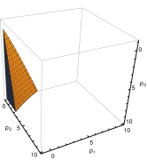
(a) $\alpha=1$

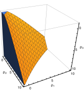
(b) $\alpha=2.5$

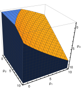
(c) $\alpha=5$

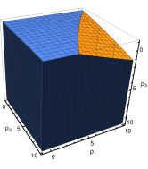
(d) $\alpha=10$

Figure 1: Stability regions of fixed point IV in model A for different values of “compressibility” $\alpha$. Dark blue regions stand for volumes in the three-dimensional parameter space spanned by $\rho_{1},\rho_{2}$ and $\rho_{3}$, where the stability matrix has positive eigenvalues.

A cumbersome explicit expression for eigenvalue $\Omega_{4}$ is not provided here. Instead, we consider a smooth section of the hypersurface determined by the equation

$$\Omega_{4}(\rho_{1},\rho_{2},\rho_{3},\alpha)=0$$

at given value of compressible parameter $\alpha$. Points belonging to the volume

$${\mathcal{B}}=\{\rho_{i}>-1\,(i=1,2,3),\alpha>0:\Omega_{4}(\rho_{1},\rho_{2},\rho_{3},\alpha)>0\}$$ (38)

determine the IR stability region. Volume $|{\mathcal{B}}|$ for four typical values of $\alpha$ is depicted in Fig. 1. $|{\mathcal{B}}|$ vanished fo the incompressible fluid and increases indefinitely with compressible parameter $\alpha$. A change of the anisotropy parameters ($\rho_{1},\rho_{2},\rho_{3}$) at fixed $\alpha$ may affect the IR stability of the fixed point according to Fig. 1. Also, it is worth mentioning that anisotropy of a mixing flow does not affect the type of critical asymptotics in both incompressible ($\alpha=0$) and infinitely compressible ($\alpha=\infty$) case. For the finite values of compressibility parameter $\alpha$ the anisotropy is an important factor in establishing scaling regimes. This clearly displays the failure of the Kolmogorov hypothesis (that the anisotropy dies out in the inertial range) in the case of critical fluids. In a vicinity of the point $\rho_{1}=\rho_{2}=\rho_{3}=0$ at fixed $\alpha$ weak anisotropy does not change IR stability.

Let us summarize main findings about obtained scaling regimes in model A that correspond to fixed point IV:

1. Regime $1$. Incompressibility of the system entails that fluid is far from a critical or phase transition point. Hence, long-wave fluctuations of the order parameter do not determine large-scale behavior. They are suppressed by the transversal turbulent fluctuations, which play a crucial role in the realization of IR scaling.

2. Regime $2$ without the inclusion of case $(e)$. In these cases the order parameter fluctuations are still weaker in comparison to the velocity ones. We can observe (items $(b),(f),(g)$) that the transversal part ($\rho_{1},\rho_{2}$) of the turbulent fluctuations inhibits the role of isotropic ($\rho_{3}=0$) longitudinal components for all permissible $\alpha$. On the other hand, in regimes $(a)$,$(c)$,$(d)$, and $(h)$ the transversal and longitudinal parts become equally relevant.

3. Regime $3$ and the case $(e)$. These regimes correspond to a strong compressible fluid. It has been mentioned above that compressibility grows very fast in the vicinity of the critical point, where fluctuations of the order parameter could not be neglected.

4.2 Model DP

Let us now analyze scaling regimes of the DP model (12). This is given by fixed points’ solution of the set of equations (22)-(25).

1. Trivial (Gaussian) fixed point

   $$g_{1}^{*} =g_{2}^{*}=0,\quad\Omega=\left[0,\,0,\,-\varepsilon,\,-\delta\right].$$ (39)

   Similarly to the case of model A, this fixed point represents the free FP for which all interactions are irrelevant and values of parameters $a$ and $b$ do not change its stability region. As expected this fixed point is stable above space dimension $d_{c}=4$ and negligible velocity fluctuations.

2. Non-equilibrium thermal fluctuations

   $$g_{1}^{*} =2\,\varepsilon\sqrt{b+1}/3,\quad a^{*}=1/2,\quad g_{2}^{*}=0,$$ (40)

   $$\Omega =\left[\varepsilon,\,\varepsilon/12-\delta,\,0,\,\varepsilon/6\right].$$ (41)

   In this regime, the stochastic velocity fluctuations are irrelevant and charge $b$ is not fixed. This regime corresponds to a pure DP model. For more details and discussions of this regime see tauber .

3. Turbulent mixing of a passive scalar

   $$g_{2}^{*} =\frac{24\,\delta}{\left\{\alpha(6+\rho_{3})+5\rho_{1}+\rho_{2}+18\right\}}, g_{1}^{*} =0,$$ (42)

   $$b^{*} =\frac{2\,\{\alpha\rho_{3}-\rho_{1}+7\rho_{2}\}}{\left\{\alpha(6+\rho_{3})+5\rho_{1}+\rho_{2}+18\right\}},$$ (43)

   $$\Omega =\left[\Omega_{1},\,\delta,\,\delta,\,0\right],$$ (44)

   where $\Omega_{1}={\partial\beta_{g}}/{\partial g}|_{\kappa=\kappa^{*}}$. This fixed point is similar to regime III of model A given by coordinates (32-34). Once again DP non-linearities are completely suppressed by vigorous turbulent fluctuations. Similarly, the parameter $a$ is not fixed.

4. Interaction of thermal and hydrodynamic fluctuations

   $$g_{1}^{*} ,\quad g_{2}^{*},\quad a^{*}=1/2,$$ (45)

   $$b^{*} =\frac{2\,\{\alpha\rho_{3}-\rho_{1}+7\rho_{2}\}}{\left\{\alpha(6+\rho_{3})+5\rho_{1}+\rho_{2}+18\right\}},$$ (46)

   $$\Omega =\left[2\,\Omega_{4},\,\Omega_{2},\,\Omega_{2},\,\Omega_{4}\right],$$ (47)

   where $\Omega_{4}={\partial\beta_{a}}/{\partial a}|_{\kappa=\kappa^{*}}$, $\Omega_{2}={\partial\beta_{g_{2}}}/{\partial g_{2}}|_{\kappa=\kappa^{*}}$. One can show that $\Omega_{2}>0$ for $\forall\rho_{1},\,\rho_{2},\,\rho_{3},\,\alpha$. Expressions for fixed point’s coordinates $g_{1}^{*}$ and $g_{2}^{*}$ can be derived from Eqs. (22)-(25), and their explicit form can be found in Appendix A, see Eq. (61).

Possible regimes at asymptotic values of ($\rho_{1},\rho_{2},\rho_{3},\alpha$) for fixed point IV can be summarized as follows:

1. ${\alpha=0}$ – unstable for any $\rho_{1},\rho_{2},\rho_{3}$

2. $0<\alpha<\infty$

   1. ${\rho_{1}\sim\rho_{2}\sim\rho_{3}\rightarrow\infty}$,
      stable for $\alpha>30\,(2+\sqrt{3})/(14-5\,\sqrt{3})\approx 20.96$

   2. ${\rho_{1}\sim\rho_{2}\rightarrow\infty,\rho_{3}=0}$, unstable for any $\alpha$

   3. ${\rho_{1}\sim\rho_{3}\rightarrow\infty,\rho_{2}=0}$,
      stable for $\alpha>(505+60\,\sqrt{70})/121\approx 8.32$

   4. ${\rho_{2}\sim\rho_{3}\rightarrow\infty,\rho_{1}=0}$,
      stable for $\alpha>30\,(2+\sqrt{3})/(14-5\,\sqrt{3})\approx 20.96$

   5. ${\rho_{1}=\rho_{2}=0,\rho_{3}\rightarrow\infty}$, stable for any $\alpha$

   6. ${\rho_{1}=\rho_{3}=0,\rho_{2}\rightarrow\infty}$, unstable for any $\alpha$

   7. ${\rho_{2}=\rho_{3}=0,\rho_{1}\rightarrow\infty}$, unstable for any $\alpha$

   8. ${\rho_{1}=\rho_{2}=\rho_{3}=0}$, stable for $\alpha>5$ (see an7 )

3. $\alpha=\infty$ – stable for any $\rho_{1},\rho_{2},\rho_{3}$.

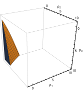
(a) $\alpha=2.5$

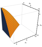
(b) $\alpha=5$

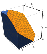
(c) $\alpha=10$

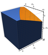
(d) $\alpha=20$

Figure 2: Stability regions of fixed point IV in model DP for different values of “compressibility” $\alpha$. Dark blue regions stand for volumes in the three-dimensional parameter space spanned by $\rho_{1},\rho_{2}$ and $\rho_{3}$, where the stability matrix has positive eigenvalues.

The volume

$${\mathcal{B}}=\{\rho_{i}>-1(i=1,2,3),\alpha>0:\Omega_{4}(\rho_{1},\rho_{2},\rho_{3},\alpha)>0\}$$ (48)

of IR stable points is displayed in Fig. 2. An analysis of this regime reveals that turbulence has similar qualitative effects on the behavior of both model A and model DP despite a different nature and origin of systems they describe.

Let us consider the stability of the regimes in a case when anisotropy function $c(\varphi)>0$ (10) is an arbitrary one. Direct calculations lead to the following relation at $\varepsilon=1$, $\delta_{K}=4/3$:

$$\Omega_{4}\sim\int_{0}^{1}\left[\frac{3}{\sqrt{b^{*}t+1}}-\frac{5}{b^{*}+4}\right]c(t)\,(1-t)^{1/2}\,t^{-1/2}{\mathrm{d}}t,$$ (49)

where $t=\cos(\varphi)^{2}$. There is no doubt that in the physical region $b^{*}>0$ eigenvalue $\Omega_{4}$ is positive. We can conclude that regardless of anisotropy intensity and structure of function $c(\varphi)$ turbulent fluctuations do not change a type of IR regime in the infinitely compressible system. They affect only the values of critical exponents.

5 Critical exponents

Green functions of the theory contain an essential physical information about a state of the system. In particular, in the percolation process the radius of gyration $R(t)$ for the spreading cloud of the agent that started from the origin at time $t^{\prime}=0$ can be expressed through the linear response function

$${R^{2}(t)} =\frac{\int|\bm{x}|^{2}\,G(|\bm{x}|,t)\,{\mathrm{d}}^{d}x}{2d\int\,G(|\bm{x}|,t)\,{\mathrm{d}}^{d}x},$$ (50)

$$G(|\bm{x}|,t) =\langle\varphi(t,\bm{x})\varphi^{\prime}(0,{\bm{0}})\rangle.$$ (51)

The RG analysis yields the following IR asymptotic solution for the response function

$$G(|\bm{x}|,t)=|\bm{x}|^{-\Delta_{\phi}-\Delta_{\phi^{\prime}}}\,f(|\bm{x}|\,t^{-1/\Delta_{\omega}}),$$ (52)

where $f$ is a scaling function (it also depends on $\alpha,\rho_{i}$ and the angle between $\bm{x}$ and $\bm{n}$), $\Delta_{\varphi}=d/2+\gamma^{*}_{\varphi},\Delta_{\varphi^{\prime}}=d/2+\gamma^{*}_{\varphi^{\prime}}$ are the scaling dimensions of fields, and $\Delta_{\omega}=2-\gamma^{*}_{\lambda}$ is the scaling dimension of frequency or a dynamical critical exponent nav1 . The additive $\gamma_{j}$ is a so-called anomalous dimension corresponding to a parameter or field $j$. Such $\gamma_{j}$ originates during the renormalization process. Symbol ^∗ denotes a value of anomalous dimensions at a fixed point. As the result, we get a power-law asymptotic expression for $R^{2}(t)$

$$R^{2}(t)\sim t^{z_{s}},\quad z_{s}=\frac{2}{\Delta_{\omega}}.$$ (53)

Let us note that in contrast to turbo , radius of gyration (50) is defined in a different way. The denominator in this expression corresponds to a number of active particles generated by a single seed at initial time. Thus, Eq. (50) represents the mean squared radius on one active particle at a given time.

The scaling behavior for a number of active particles

$${N(t)}=\int\,G(|\bm{x}|,t)\,{\mathrm{d}}^{d}x$$ (54)

is given by the asymptotic relation

$$N(t)\sim t^{\theta_{s}},\quad\theta_{s}=-\frac{(\gamma^{*}_{\varphi}+\gamma^{*}_{\varphi^{\prime}})}{\Delta_{\omega}}.$$ (55)

A one-loop RG calculation leads to the expressions

$$\gamma_{\varphi}+\gamma_{\varphi^{\prime}} =-\frac{g_{1}}{4\,\sqrt{\beta+1}},$$ (56)

$$\gamma_{\lambda} =\frac{g_{2}}{24}\left\{\alpha(6+\rho_{3})+5\rho_{1}+\rho_{2}+18\right\}+\frac{g_{1}}{8\sqrt{b+1}}.$$ (57)

Using these functions and coordinates of the fixed point IV one can obtain the exponents $z_{s}$ and $\theta_{s}$ at given values of the parameters $(\alpha,\rho_{1},\rho_{2},\rho_{3})$ in the form of $(\epsilon,\delta)$-expansion up to the first order. Let us consider a case of weak anisotropy $\rho_{1}\sim\rho_{2}\sim\rho_{3}\ll 1$ at $\varepsilon=1,\delta=4/3$ for regime IV. Then the exponent $\theta_{s}$ can be represented as a segment of power series in $\rho_{j}$

$$\theta_{s}=\frac{\alpha-5}{6\,(2\alpha+5)}-\frac{5\alpha\,(\rho_{1}+\rho_{2}-\rho_{3})}{8\,(2\alpha+5)^{2}}+{\mathcal{O}}(\rho_{j}^{2}),$$ (58)

and $z_{s}=2/(2-\delta)=3$. This relation is universal, i.e. it does depend neither on large-scale anisotropy nor compressibility of the medium. In the previous section, it has been established that regime IV is unstable at small values of $\alpha$ and stable at its large values. Therefore, it is reasonable to consider expression (58) at large $\alpha$ (formally for $\alpha\gg 5/2$)

$$\theta_{s}=\frac{1}{12}-\frac{5\,(4+\rho_{1}+\rho_{2}-\rho_{3})}{32\,\alpha}+{\mathcal{O}}(\alpha^{-2}).$$ (59)

The term $(4+\rho_{1}+\rho_{2}-\rho_{3})$ is positive, at least in the range $|\rho_{j}|\leqslant 1$. Thus corrections to the exponent $\theta_{s}$ due to weak anisotropy and finite compressibility reduce values of $\theta_{s}$. At this point we can conclude that number $N(t)$ of active particles grows slower than in the case of isotropic and incompressible systems.

The IR stable regime III leads to the exact qualitative outcomes $z_{s}=2/(2-\delta)=3,\,\theta_{s}=0$, this is consistent with known Richardson’s 4/3 power law of turbulent diffusion $\partial_{t}R^{2}(t)\sim R^{4/3}(t)$ turbo .

6 Conclusion

An experimental study of critical fluids in terrestrial-like environment faces influence of Earth gravity inducing a distinguished direction due to compressibility under the hydrostatic pressure. Systems are subject to mixing, shaking and other hydrodynamic effects in laboratory conditions. Our analysis has been focused on the investigation of possible stable regimes in anisotropic turbulently moving critical fluids described by the A and DP effective models. The renormalization group analysis within the framework of the one-loop approximation allows us to draw the following conclusions and describe the major findings

1. At a qualitative level both model A and model DP coupled to the Kraichnan model manifest the same scaling behavior.

2. Close to criticality the effect of anisotropy could be relevant for establishing scaling behavior. This result could call into a question well-established and universal assumptions that large-scale anisotropy is irrelevant in the inertial range. A critical liquid remains sensitive to a distinguished direction ${\bm{n}}$, what implies that the Kolmogorov hypothesis does not apply to a critical fluid.

3. Within the considered models, regime IV in a strong compressible system is less sensitive to the anisotropy of a fully developed turbulent flow. The existence of large scale anisotropy does not affect its stability at the limit values of $\alpha=\infty$ (see Sec. IV, item (iii)). In the infinitely (formally) compressible system, in which longitudinal velocity fluctuations prevail due to large values of bulk viscosity, regimes stability also does not depend on the specific form of the function $c(\varphi)$, see Eq. (49). At the same time, quantitative values of critical exponents are not universal. In fact, they are determined by function $c(\varphi)$.

4. In the intermediate range of $\alpha$, weak (linear in $\rho_{j}$) anisotropy fluctuations do not change the regimes. An increase of anisotropy is accompanied by the complex pattern of interaction between transversal and longitudinal turbulent fluctuations and the long-wavelength critical fluctuations of the order parameter, as depicted in Figs. 1, and 2. Here, anisotropy plays a crucial role imposing lower limits on the value of $\alpha$ (on the “compressibility degree”, see Secs. 4.1, and 4.2 and item denoted as IV therein). This result is in agreement what we can physically anticipate: order parameter fluctuations are strong in the vicinity of the critical point, where compressibility is large enough.

5. Having calculated the anomalous dimensions (56), and (57), we have estimated the critical exponents at given $\rho_{j}$ and $\alpha$ (58), and (59). The compressibility and anisotropy alter values of the critical exponent. Whereas compressibility reduces the magnitude of the critical exponents, according to the expression (59), the effect of anisotropy is more subtle and twofold, depending on the sign of the value $\rho_{1}+\rho_{2}-\rho_{3}$.

The effect of compressibility on critical behavior of an isotropic system was revealed by the authors of work an7 , where a new scaling regime IV has been identified. However, our analysis shows that not only compressibility but also large-scale anisotropy may control the stability of the critical regimes and alter the quantitative results.

Appendix A Coordinates of fixed points

Here, we present explicit expressions for coordinates of nontrivial fixed points. First, at nontrivial fixed point IV of model A charge $g_{1}$ has the following coordinate

$$g_{1}^{*}=\frac{\sqrt{b+1}}{3A}\left(A\,\varepsilon-2A\,\delta+18B\,\delta\right).$$ (60)

At nontrivial fixed point IV of model DP fixed points’ values of charges $g_{1}$ and $g_{2}$ are given by the following expressions

$$g_{1}^{*} =\frac{4\sqrt{b+1}}{A+9B}\left(A\,\varepsilon-2A\,\delta+18B\,\delta\right),$$ (61)

$$g_{2}^{*} =\frac{12\,(4\,\delta-\varepsilon)}{A+9B}.$$ (62)

In Eqs. (60)-(62) we have used the following abbreviations

$$A =\alpha(6+\rho_{3})+5\rho_{1}+\rho_{2}+18,$$

$$B =\frac{\alpha}{{b^{*}}^{2}}\left[2(\sqrt{b^{*}+1}-1)(b^{*}-\rho_{3})+b^{*}\rho_{3}\right].$$

The fixed point value $b^{*}$ is given by Eq. (36) or Eq. (46), respectively.

References

- [1] P. C. Hohenberg and B. I. Halperin. Rev. Mod. Phys., 49:435, 1977.
- [2] D. Yu. Ivanov. Critical Behaviour of Non-Ideal Systems. Wiley-VCH, Weinhein, 2008.
- [3] P. K. Khabibullaev and A. A. Saidov. Phase Separation in Soft Matter Physics: Micellar Solutions, Microemulsions, Critical Phenomena. Springer Series in Solid-State Sciences, Weinhein, 2003.
- [4] M. A. Anisimov. Critical Phenomena in Liquids and Liquid Crystals. Gordon and Breach, Amsterdam, 1991.
- [5] M. Barmatz, H. Inseob, J. A. Lipa, and R. V. Duncan. Rev. Mod. Phys., 79:1, 2007.
- [6] R. F. Berg and M. R. Moldover. J. Chem. Phys., 93(3):1926, 1990.
- [7] H. K. Janssen. Phys. Rev. E, 55:6253, 1997.
- [8] P. A. Davidson. Turbulence: An Introduction for Scientists and Engineers (2nd edition). Oxford University Press, 2015.
- [9] U. Frisch. Turbulence: The Legacy of A. N. Kolmogorov. Cambridge University Press, Cambridge, 1995.
- [10] A. S. Monin and A. M. Yaglom. Statistical Fluid Mechanics, volume 2. MIT Press, Cambridge, MA, 1975.
- [11] G. Falkovich, K. Gawedzki, and M. Vergassola. Rev. Mod. Phys., 73:913, 2001.
- [12] L. Ts. Adzhemyan, N. V. Antonov, and A. N. Vasil’ev. The Field Theoretic Renormalization Group in Fully Developed Turbulence. Gordon and Breach, Amsterdam, 1999.
- [13] M. Hnatič, J. Honkonen, and T. Lučivjanský. Acta Physica Slovaca, 66:69, 2016.
- [14] R. H. Kraichnan. Phys. Rev. Lett., 72:1016, 1994.
- [15] M. Chertkov, I. Kolokolov, and M. Vergassola. Phys. Rev. E., 56:5483, 1997.
- [16] L. Ts. Adzhemyan and N. V. Antonov. Phys. Rev. E., 58:7381, 1998.
- [17] N. V. Antonov. Phys. Rev. E., 60:6691, 1999.
- [18] A. N. Vasil’ev. The Field Theoretic Renormalization Group in Critical Behavior Theory and Stochastic Dynamics. Chapman and Hall, Boca Raton, 2004.
- [19] E. Jurčišinová, M. Jurčišin, and R. Remecký. Phys. Rev. E, 80:046302, 2009.
- [20] A. Z. Patashinskii and V. L. Pokrokovskii. Fluctuation Theory of Phase Transitions. Pergamon Press, Oxford, 1979.
- [21] R. H. Kraichnan. Phys. Fluids, 11:945, 1968.
- [22] N. V. Antonov. J. Phys. A: Math. Gen., 39(25):7825, 2006.
- [23] S. N. Shore. Astrophysical Hydrodynamics:An Introduction. Wiley-VCH Verlag GmbH& KGaA, Weinheim, 2007.
- [24] J. Kim and D. Ryu. Astrophys. J., 630:L45, 2005.
- [25] F. Sahraoui, M. L. Goldstein, P. Robert, and Yu. V. Khotyainstsev. Phys. Rev. Lett., 102:231102, 2009.
- [26] S. Galtier and S. Banerjee. Phys. Rev. Lett., 107:134501, 2011.
- [27] S. Banerjee and S. Galtier. Phys. Rev. E, 87:013019, 2013.
- [28] S. Banerjee, L. Z. Hadid, F. Sahraoui, and S. Galtier. Astrophys. J. Lett., 829:L27, 2016.
- [29] L. Z. Hadid, F. Sahraoui, and S. Galtier. Astrophys. J., 838:9, 2017.
- [30] A. Celani, A. Lanotte, A. Mazzino, and M. Vergassola. Phys. Rev. Lett., 84:2385, 2000.
- [31] S. G. Saddoughi and S. V. Veeravalli. J. Fluid. Mech., 268:333, 1994.
- [32] I. Arad, B. Dhruva, S. Kurien, V. S. L’vov, I. Procaccia, and K. R. Sreenivasan. Phys. Rev. Lett., 81:5330, 1998.
- [33] R. Rubinstein and J. M. Barton. Phys. Fluids, 30:2987, 1987.
- [34] L. Ts. Adzhemyan, N. V. Antonov, M. Hnatič, and S. V. Novikov. Phys. Rev. E, 63:016309, 2000.
- [35] D. Carati and L. Brenig. Phys. Rev. A, 40:5193, 1989.
- [36] T. L. Kim and A. V. Serdyukov. Theor. Math. Phys., 105:1525, 2005.
- [37] J. Zinn-Justin. Quantum Field Theory and Critical Phenomena. 4th edition, Oxford University Press, Oxford, 2002.
- [38] D. J. Amit and V. Martín-Mayor. Field Theory, the Renormalization Group and Critical Phenomena. World Scientific, Singapore, 2005.
- [39] K. G. Wilson and J. Kogut. Phys. Rep., 12:75, 1974.
- [40] Jean Zinn-Justin. Phase transitions and renormalization group. Clarendon, 2007.
- [41] F. Wegner. Phase Transitions and Critical Phenomena, Volume 6 (C. Domb and M. S. Green, eds.). Academic Press, London and New York, 1976.
- [42] G. Parisi. J. Stat. Phys., 23:49, 1980.
- [43] J. C. Le Guillou and J. Zinn-Justin. Phys. Rev. B, 21:3976, 1980.
- [44] A. Pelissetto and E. Vicari. Phys. Reports, 368:549, 2002.
- [45] H. Kleinert and V. Schulte-Frohlinde. Critical Properties of Theories. World Scientific, Singapore, 2001.
- [46] M. V. Kompaniets and E. Panzer. Phys. Rev. D, 96:036016, 2017.
- [47] L. Ts. Adzhemyan, N. V. Antonov, M. V. Kompaniets, and A. N. Vasil’ev. Int. Journ. Mod. Phys. B, 17:2137, 2003.
- [48] N. V. Antonov and A. N. Vasil’ev. Theor. Math. Phys., 60:671, 1984.
- [49] L. Ts. Adzhemyan, S. V. Novikov, and L. Sladkoff. Vestnik of St. Petersburg University, 4:109, 2008.
- [50] L. Ts.Adzhemyan, N. V. Antonov, V. A. Barinov, Yu. S. Kabrtits, and A. N. Vasil’ev. Phys. Rev. E, 64:056306, 2001.
- [51] B. Delamotte. An Introduction to the Nonperturbative Renormalization Group. In Schwenk A., Polonyi J. (eds) Renormalization Group and Effective Field Theory Approaches to Many-Body Systems. Lecture Notes in Physics, vol 852. Springer, Berlin, Heidelberg, 2012.
- [52] J. Polonyi. Central Eur. J. Phys., 1:1, 2003.
- [53] L. Canet and H. Chate. J. Phys. A: Math. Gen., 40:1937, 2007.
- [54] L. Canet, B. Delamotte, and N. Wschebor. Phys. Rev. E, 93:063101, 2016.
- [55] C. Pagani. Phys. Rev. E, 92:033016, 2015.
- [56] U. C. Täuber. Critical Dynamics. A Field Theory Approach to Equilibrium and Non-Equilibrium Scailing Behavior. Cambridge University Press, Cambridge, 2014.
- [57] R. Kubo. Rep. Prog. Phys., 29:255, 1966.
- [58] N. G. van Kampen. Stochastic processes in Physics and Chemistry. North-Holland, Amsterdam, 2007.
- [59] Géza Ódor. Phys. Rev. E, 70(2):26119, aug 2004.
- [60] Uwe Claus Täuber, Martin Howard, and Benjamin P. Vollmayr-Lee. J. Phys. A: Math. Gen., 38:R79–R129, 2005.
- [61] B. Schmittmann and R. K. P. Zia. Statistical mechanics of driven diffusive systems, volume 17 of Phase transitions and critical phenomena. Academic Press, 1995.
- [62] D. C. Mattis and M. L. Glasser. Rev. Mod. Phys., 70:979, 1998.
- [63] H. Hinrichsen. Adv.Phys., 49:815, 2000.
- [64] H. K. Janssen and U. C. Täuber. Ann.Phys., 315:147, 2004.
- [65] M. Henkel, Haye Hinrichsen, and S. Lübeck. Non-Equilibrium Phase Transitions: Volume 1-Absorbing Phase Transitions. Springer, 2008.
- [66] S. R. Broadbent and I. M. Hamersley. Proc. Camb. Phil. Soc., 53(3):629, 1957.
- [67] U. C. Täuber. Adv. Solid State Phys., 43:629, 2003.
- [68] N. V. Antonov, M. Hnatič, A. S. Kapustin, T. Lučivjanský, and L. Mižišin. Phys. Rev. E., 93:012151, 2016.
- [69] M. Dančo, M. Hnatič, T. Lučivjanský, and L. Mižišin. Theor. Math. Phys., 176:79, 2013.
- [70] N. Antonov, A. Ignatieva, and A. Malyshev. Physics of Particles and Nuclei, 41:998, 2010.
- [71] H. K. Janssen, K. Oerding, F. van Wijland, and H. J. Hilhorst. Eur. Phys. J. B, 7:137, 1999.
- [72] H. K. Janssen and O. Stenull. Phys. Rev. E, 78:061117, 2008.
- [73] C. W. Gardiner. Handbook of Stochastic Methods: For Physics, Chemistry, and the Natural Sciences. Springer, 2009.
- [74] N. V. Antonov, A. S. Kapustin, and A. V. Malyshev. Theor. Math. Phys., 169:1470, 2011.
- [75] R. Folk and G. Moser. J. Phys. A: Math. Gen., 39:207, 2006.
- [76] N. V. Antonov. Physica D, 144(3–4):370–386, 2000.
- [77] N. V. Antonov and A. S. Kapustin. J. Phys. A: Math. Gen., 43:405001, 2010.
- [78] Maplesoft. Maple. Waterloo Maple Inc., Waterloo, Ontario, Canada, 2012.