Stochastic Multipath Model for the In-Room Radio Channel based on Room Electromagnetics

Abstract

We propose a stochastic multipath model for the received signal for the case where the transmitter and receiver, both with directive antennas, are situated in the same rectangular room. This scenario is known to produce channel impulse responses with a gradual specular-to-diffuse transition in delay. Mirror source theory predicts the arrival rate to be quadratic in delay, inversely proportional to room volume and proportional to the product of the antenna beam coverage fractions. We approximate the mirror source positions by a homogeneous spatial Poisson point process and their gain as complex random variables with the same second moment. The multipath delays in the resulting model form an inhomogeneous Poisson point process which enables derivation of the characteristic functional, power/kurtosis delay spectra, and the distribution of order statistics of the arrival delays in closed form. We find that the proposed model matches the mirror source model well in terms of power delay spectrum, kurtosis delay spectrum, order statistics, and prediction of mean delay and rms delay spread. The constant rate model, assumed in e.g. the Saleh-Valenzuela model, is unable to reproduce the same effects.

I Introduction

Stochastic models for multipath channels are useful tools for the design, analysis and simulation of systems for radio localization and communications. These models allow for tests via Monte Carlo simulation and in many cases provide analytical results useful for system design. Numerous such models exist for the complex baseband representation of the signal at the receiver antenna (omitting any additive terms due to noise or interference)

$$y(\tau)=\sum_{k}\alpha_{k}s(\tau-\tau_{k}),$$ (1)

where $s(t)$ is the complex baseband representation of the transmitted signal and the term due to path $k$ has complex gain $\alpha_{k}$ and delay $\tau_{k}$. The received signal is fully described as a marked point process

$$\mathcal{X}=\{(\tau_{0},\alpha_{0}),(\tau_{1},\alpha_{1}),(\tau_{2},\alpha_{2}),\dots\}.$$ (2)

A models of this structure was studied in the pioneering work by Turin [1] in which $\mathcal{X}$ can be seen as a marked Poisson point process specified by parameters determining the arrival rate $\lambda(\tau)$ and the mark density $p(\alpha|\tau)$. Although Turin’s model was originally intended for urban radio channels, it has since been taken as a the basis for a wide range of models for outdoor and indoor channels including the clustered models by Suzuki [2], Hashemi [3], Saleh and Valenzuela [4], Spencer et al. [5] and Zwick et al. [6, 7]. More recently, this type of statistical channel models has been considered for ultrawideband [8, 9] and for millimeter-wave spectrum [10, 11, 12] systems. To make use of the model, the arrival rate and mark density should be defined. These settings are critical since they determine channel parameters relavant for system design such as the distribution of instantaneous mean delay and rms delay spread.

Commonly, the arrival rate (within a cluster) is assumed constant while the second moment of the mark density is assumed to follow an exponential decay [4, 5, 6, 7, 10, 8, 9, 11, 12]. The “constant rate” model is appealing since it requires only one single parameter, i.e. the arrival rate, to be determined empirically. Usually a two-step procedure is followed: first the points of the hidden process $\mathcal{X}$ are estimated from observations of $y(t)$ and then the arrival rate is estimated from there (e.g. relying on interarrival times). The first step of this method is prone to censoring effects as discussed in [13]. In the presense of noise, the weaker components predominantly arriving at large delays may be undetected. A similar effect occurs if the measurement bandwidth is insufficient to distinguish signal components with short interarrival times. If unaccounted for, both of these censoring effects lead to underestimation of the arrival rate. As noted in [14], several authors justify the constant rate assumption qualitatively as a “convenient compromise” between the increasing number of possible multipath components and the increasing shadowing probability. Nevertheless, as also noted in [14], there seems to be no principal reason that the effects should balance each other out to produce exactly a constant rate.

In some cases, stochastic multipath models relying on the constant rate model do not agree well with measurements at all. This is particularly true for inroom propagation channel, which has been explored in a number of works including [15, 16, 17, 18, 19, 20, 21, 22, 23]. There the received signal exhibits a gradual diffusion from specular at early delays to diffuse at later delays. This effect is not captured in the constant rate model. Moreover, in clustered models, the cluster arrival rate is assumed constant yielding a total path arrival rate which increases linearly with delay [24]. This increase is, however, too slow compared to the power decay to account for the specular-to-diffuse transition.

For the inroom scenario, an alternative to the constant rate assumption was proposed in [23]. The model is based on mirror source analysis of the case where the transmitter and receiver antennas are both directive and sit within the same rectangular room with flat walls. For this setup, the arrival rate (averaged over uniformly distributed transmitter antenna positions and orientations) was found to be inversely proportional to room volume, depend on antenna directivity and to increase quadratically with delay accounting for the specular-diffuse transition. The analysis also leads to closed form expressions for the variance of the mark density and the resulting power delay spectrum. The power delay spectrum decays exponentially in delay and the reverberation time (decay rate) is predicted very accurately by the Eyring model [25, 15, 26] applying Kuttruff’s correction factor [27]. The power delay spectrum is of the same form as studied and experimentally validated in [26, 28]. The analysis in [23] further revealed that while the arrival rate was easy to derive, higher order moments for the arrival process are very difficult to obtain from the mirror source theory.

In the present contribution, we propose to approximate the mirror source model in [23] using a spatial Poisson process which is more analytically tractable. The obtained model is of the same type as Turin’s model, but has the same arrival rate and power delay spectrum as the mirror source process. The approximation model permits derivation of moments and cumulants of the received signal via the characteristic and cumulant generating functionals. Thus, we derive the power (second moment) and kurtosis (ratio of fourth moment and squared second moment) of the received signal as a function of delay. The kurtosis is related to the arrival rate: in the simplifying large bandwidth case, the arrival rate is inversely proportional to the excess kurtosis of the received signal. For the proposed inhomogeneous model, the distribution of interarrival times, which has been widely studied in the channel modeling literature, turns out to be degenerate and is therefore not useful. Instead, we study the distribution of order statistics which we derived for the approximation model.

To evaluate the accuracy of the proposed Poisson approximation we compare it to Monte Carlo simulations of the mirror source model. Our simulations show that the proposed Poisson approximation captures the specular-diffuse transition and fit well the mirror source model in terms of power- and kurtosis delay spectra and order statistics for the arrival process. The distribution of instantaneous mean delay and rms delay spread agrees with the mirror source model. In these simulations we also contrast with the constant rate model. It is observed that the constant rate model is able to capture the power delay spectrum, but represents poorly the kurtosis, order statistics, instantaneous mean delay and rms delay spread. We conclude that to accurately model these parameters for in-room channels, the constant rate model is inadequate.

The paper is organized as follows. Section II defines the notation and summarizes the results of [23]. In section III we first represent the mirror source process as a spatial point process and then approximate it using a Poisson point process. Sections IV and V gives the results related to kurtosis of the received signal $y(t)$ and the distribution of order statistics for the arrival times. The accuracy of the proposed Poisson approximation is tested in numerical examples given in Section VI. Discussion and conclusions are given in VII and VIII.

II Mirror Source Process for Rectangular Room

The present contribution relies on the same setup as in the previous work [23] and utilizes the results sumarized below. For further details, the reader is referred to [23].

Consider a rectangular room with two directive antennas (one transmitter and one receiver) located inside. The room has dimension $L_{x}\times L_{y}\times L_{z}$, volume $V=L_{x}L_{y}L_{z}$ and surface area $S=2(L_{x}L_{y}+L_{y}L_{z}+L_{x}L_{z})$. Positions are given in a Cartesian coordinate system aligned such that the room spans the set $[0,L_{x})\times[0,L_{y})\times[0,L_{z})$. We assume that the carrier wavelength $l_{c}$ is small compared to the room dimensions, and that only specular reflections occur with an average gain $\mathrm{bar}g$. The positions of the transmitter and receiver are denoted by $r_{T}$ and $r_{R}$ . We subscript all entities related to the transmitter and receiver by $T$ and $R$, respectively.

Denote by $G(\Omega)$ the antenna gain in the direction specified by the three dimensional unit vector $\Omega\in\mathbb{S}_{2}$, where $\mathbb{S}_{2}$ is the unit sphere. We assume the antennas to be lossless. The footprint of an antenna on the unit sphere surrounding it is defined as $\mathcal{O}=\{\Omega:G(\Omega)\geq\epsilon\cdot G_{\max}\}$ where $G_{\max}$ is the maximum gain and $\epsilon\geq 0$ defines a gain level below which we ignore any signal contributions. The beam coverage fraction is further defined as

$$\omega=\frac{1}{4\pi}\int_{\mathbb{S}_{2}}\mathds{1}(\Omega\in\mathcal{O})d\Omega,$$ (3)

where $\mathds{1}(\cdot)$ denotes an indicator function with value one if the argument is true and zero otherwise. The beam coverage fraction ranges from zero to one and can be interpreted as the probability of a wave impinging from a uniformly random direction is within the antenna beam.

The mirror sources (and thus the propagation paths) are indexed by a triplet $k=(k_{x},k_{y},k_{z})$. Mirror source $k$ has position

$$r_{T(k_{x},k_{y},k_{z})}=\begin{bmatrix}\big{\lceil}\tfrac{k_{x}}{2}\big{\rceil}\cdot 2L_{x}+(-1)^{k_{x}}\cdot x_{T}\\ \big{\lceil}\tfrac{k_{y}}{2}\big{\rceil}\cdot 2L_{y}+(-1)^{k_{y}}\cdot y_{T}\\ \big{\lceil}\tfrac{k_{z}}{2}\big{\rceil}\cdot 2L_{z}+(-1)^{k_{z}}\cdot z_{T}\end{bmatrix}.$$ (4)

Further interpretation of the mirror source index is given in [23]. By replacing subscript $T$ by subscript $R$ in (4), gives the position $r_{Rk}$ of mirror receiver $k$. Propagation path $k$ has delay

$$\tau_{k}=\|r_{Tk}-r_{R}\|/c=\|r_{Rk}-r_{T}\|/c,$$ (5)

where $c$ is the speed of light. For path $k$ the direction of arrival reads

$$\Omega_{Rk}=\frac{r_{Tk}-r_{R}}{\|r_{Tk}-r_{R}\|}.$$ (6)

The direction of departure denoted by $\Omega_{Tk}$ follows from (6) by interchanging subscripts $T$ and $R$. The power gain of path $k$ is specified as

$$|\alpha_{k}|^{2} =\mathrm{bar}g^{|k|}\cdot\frac{G_{T}(\Omega_{Tk})G_{R}(\Omega_{Rk})}{(4\pi c\tau_{k}/l_{c})^{2}}$$ (7)

with the convention $|k|=|k_{x}|+|k_{y}|+|k_{z}|$.

Randomness is introduced to the mirror source model by letting the transmitter’s position be independent and uniformly distributed random variables. The arrival count $N(\tau)$, is a random counting variable designating the number of received (non-zero) signal components with delay less than or equal to $\tau$. The mean arrival count reads

$$\mathbb{E}[N(\tau)]=\frac{4\pi c^{3}\tau^{3}}{3V}\omega_{T}\omega_{R}\mathds{1}(\tau>0)$$ (8)

with the corresponding arrival rate

$$\lambda(\tau)=\frac{d\mathbb{E}[N(\tau)]}{d\tau}=\frac{4\pi c^{3}\tau^{2}}{V}\omega_{T}\omega_{R}\mathds{1}(\tau>0).$$ (9)

Assuming the complex gains to be uncorrelated random variables, the second moment of the received signal can be written in terms of the delay power spectrum $P(t)$ as

$$\mathds{E}[|y(\tau)|^{2}]=\int_{-\infty}^{\infty}P(\tau-t)|s(t)|^{2}dt.$$ (10)

The delay power spectrum can be obtained as a product of the arrival rate $\lambda(\tau)$ and the conditional second moment of the complex gains $\sigma_{\alpha}^{2}(\tau)=\mathbb{E}[|\alpha|^{2}|\tau]$, i.e.

$$P(\tau)=\sigma_{\alpha}^{2}(\tau)\lambda(\tau).$$ (11)

With close approximation, the conditional second moment is

$$\sigma_{\alpha}^{2}(\tau) =\frac{1}{c^{2}\tau^{2}\omega_{T}\omega_{R}}\cdot\exp(-\tau/T).$$ (12)

with the reverberation time defined according to Eyring’s model [25]

$$T=-\frac{4V\xi}{cS\ln(\mathrm{bar}g)},$$ (13)

where Kuttruff’s correction factor [27] is

$$\xi=\frac{1}{1+\gamma^{2}\ln(g)/2}.$$ (14)

Here, the constant $\gamma^{2}$ depends on the aspect ratio of the room and can be found from Monte Carlo simulations. It typically ranges from 0.3 to 0.4 [27]. The resulting power delay spectrum reads

$$P(\tau)=\mathds{1}(\tau>0)\cdot\frac{4\pi c}{V}\cdot\exp(-\tau/T).$$ (15)

Notice that the antennas do not enter in (15).

III The Mirror Source Process as a Spatial Point Process

The mirror source model can be studied by viewing the positions of the mirror sources

$$\mathcal{M}=\{r_{Tk}:k\in\mathbb{Z}^{3}\}.$$ (16)

as a spatial point process in $\mathbb{R}^{3}$. Each point $r_{Tk}\in\mathcal{M}$ is uniformly distributed within its own“mirror room” and there is exactly one point per mirror room. This makes $\mathcal{M}$ a homogeneous point process with intensity

$$\varrho_{\mathrm{m}}(r)=1/V,\quad r\in\mathbb{R}^{3}.$$ (17)

Clearly, $\mathcal{M}$ is a random point process with much more structure than the familiar spatial Poisson point process. Indeed, given any of the points in the process, all other points are known perfectly. In contrast hereto, since the points of a Poisson process are independent, knowledge of one point gives no information of the presence or location of other points.

Due to the directive antennas, some of the mirror sources may not contribute to the received signal, and are hence considered ’invisible’. We consider a path as ’visible’ if and only if both the direction of departure and the direction of arrival reside within the respective beam supports of the transmitter and receiver. Then the set of ’visible’ mirror sources reads

$$\mathcal{V}=\left\{r\in\mathcal{M}:\frac{r-r_{T}}{\|r-r_{T}\|}\in\mathcal{O}_{T},\frac{r-r_{R}}{\|r-r_{R}\|}\in\mathcal{O}_{R}\right\}.$$ (18)

The intensity function of $\mathcal{V}$ can be derived by noticing that due to the assumption of uniformly distributed transmit antenna orientation, the probability for the antenna of a mirror source to be oriented toward the receiver, i.e. to have direction of departure within the beam support of transmitter antenna, is $\omega_{T}$. Furthermore, a mirror source only contributes if the direction of arrival is also within the (deterministic) beam support of the receiver antenna giving the intensity function

$$\varrho_{\mathrm{v}}(r)=\mathds{1}\left(\frac{r-r_{R}}{\|r-r_{R}\|}\in\mathcal{O}_{R}\right)\frac{\omega_{T}}{V},\quad r\in\mathbb{R}^{3}.$$ (19)

Fig.1 illustrates the two point processes $\mathcal{M}$ and $\mathcal{V}$. The process $\mathcal{V}$ is a subset of $\mathcal{M}$ and therefore the points in $\mathcal{V}$ coincide with points in $\mathcal{M}$.

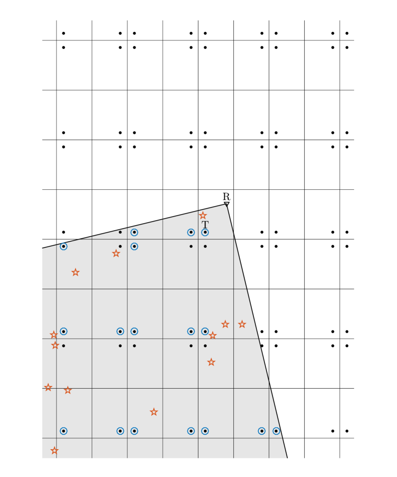
Figure 1: Realizations of the mirror source process and corresponding Poisson approximation. For readability, only sources in mirror rooms with $k_{z}=0$ are shown projected to the $x$–$y$ plane. The gray area indicates the beam coverage of the receiver antenna (R). The transmitter antenna (T) is a hemisphere oriented in the direction of the receiver. The antennas are at the same height. Black dots: Mirror source positions ($\mathcal{M}$). Blue circles: The mirror sources for which the receiver is in the beam coverage ($\mathcal{V}$). Red stars: Poisson approximation ($\mathcal{V}_{\mathrm{PPP}}$).

Relation (5) maps $\mathcal{V}$ into a one-dimensional point process on the delay axis, i.e.

$$\mathcal{T}=\{\|r-r_{R}\|/c:r\in\mathcal{V}\}.$$ (20)

Using Campbell’s theorem, the mean arrival count for $\mathcal{T}$ can be derived as

$$\mathbb{E}[N(\tau)] =\int\varrho_{\mathrm{v}}(r)\mathds{1}(\|r-r_{R}\|<c\tau)dr$$

$$=\frac{4\pi c^{3}\tau^{3}}{3V}\cdot\omega_{T}\omega_{R}\cdot\mathds{1}(\tau>0).$$ (21)

As it should, this agrees with (8) and thus the arrival rate (intensity function) $\lambda(\tau)$ of $\mathcal{T}$ is given in (9).

All information needed to evaluate the received signal using (1), can be collected in form of a marked process

$$\mathcal{X}=\{(\tau_{k},\alpha_{k}):\tau_{k}\in\mathcal{T}\},$$ (22)

with the gain given by (7).

The three point processes $\mathcal{M},\mathcal{V}$ and $\mathcal{T}$ and the marked point process $\mathcal{X}$ all have a structure reflecting their geometric construction. Given any particular point in $\mathcal{M}$, the whole realization is completely determined. Due to this structure, it is very challenging, if at all possible, to obtain second or higher order characterizations for these point processes [23]. This observation is in line the well investigated problem in stochastic geometry of counting lattice points inside a sphere with random center, see e.g. [29]. The mean is known exactly [29], but the asymptotic behaviour for the deviation from mean, including the variance, is still being investigated; the standing conjecture in the literature being that the count variable approaches a Poisson variable as the radius of the sphere increases [30, 31]. This observation, however, motivates our hypothesis that the arrival time process can be approximated adequately by Poisson point process. To evaluate the accuracy of such an approximation, we must resort to simulation studies due to the lack of a higher order characterization.

III-A Poisson Approximation for the Mirror Source Process

To facilitate analysis, we give Poisson approximations for the processes $\mathcal{M}$, $\mathcal{V}$ and $\mathcal{T}$. The point process $\mathcal{M}$ is approximated by a homogeneous Poisson point process in $\mathbb{R}^{3}$ according to

$$\mathcal{M}\approx\mathcal{M}_{\mathrm{PPP}}\sim\mathrm{PPP}(\mathbb{R}^{3},\varrho_{\mathrm{m}})$$ (23)

where the notation $\mathrm{PPP}(\cdot,\cdot)$ denotes a Poisson point process in the specified set and with the specified intensity function. To approximate $\mathcal{V}$ we account for the antennas. The transmitter antenna is accounted for by independently thinning $\mathcal{M}_{\mathrm{PPP}}$ keeping points probability $\omega_{T}$. The receiver antenna is accounted for by keeping only points with direction of arrival within the beam coverage. This procedure yields a Poisson point process $\mathcal{V}_{\mathrm{PPP}}$ with the same intensity function as $\mathcal{V}$, i.e.

$$\mathcal{V}\approx\mathcal{V}_{\mathrm{PPP}}\sim\mathrm{PPP}(\mathbb{R}^{3},\varrho_{\mathrm{v}}).$$ (24)

Fig. 1 gives an example of a realization of $\mathcal{V}_{\mathrm{PPP}}$.

Mapping the process $\mathcal{V}_{\mathrm{PPP}}$ to the delay axis as in (20) gives according to Kingman’s mapping theorem [32] a new Poisson point process with intensity function $\lambda(t)$

$$\mathcal{T}\approx\mathcal{T}_{\mathrm{PPP}}=\{\|r-r_{R}\|/c:r\in\mathcal{V}_{\mathrm{PPP}}\}\sim\mathrm{PPP}(\mathbb{R},\lambda).$$ (25)

Each point in the arrival process $\tau_{k}\in\mathcal{T}_{\mathrm{PPP}}$ is marked independently with a circular symmetric complex gain $\alpha_{k}\sim p(\alpha_{k}|\tau_{k})$ giving a marked Poisson point process

$$\mathcal{X}_{\mathrm{PPP}}=\{(\tau,\alpha):\tau\in\mathcal{T}_{\mathrm{PPP}}\}.$$ (26)

The mark density $p(\alpha|\tau)$ can be chosen in many ways as we only require that it is complex circular and has a specified variance. Owing to (11), the conditional second moment can be chosen to ensure that the power delay spectrum coincide with the mirror source model as (12). For example, we may draw independently the complex gain according to a complex circular Gaussian pdf with a specified second moment $\sigma_{\alpha}^{2}(\tau)$. Alternatively, we may draw the magnitude of $\alpha|\tau$ from an appropriate fading model (Rayleigh, Rice, log-normal, Nakagami-m, etc.) with specified second moment and the phase uniformly distributed on $[0,2\pi)$. The specific, however, choice enters in the forthcoming analysis in a way so it is straightforward to account for it. We will leave the choice open for now to achieve more generally applicable results.

The underlying Poisson process makes the approximation model analytically tractable and simple to simulate from. The approximations preserve the intensity functions, i.e. the first order properties of the processes, but no effort was put into to preserving higher order properties. From the example in Fig. 1 it is apparent, that the Poisson approximation disregards the boundaries of the mirror rooms and can result in more than one mirror source per room. This is a manifest of the fact that a Poisson process does not include second and higher-order effects, i.e. interaction between points. For example the process $\mathcal{M}$ has exactly one point in each mirror room whereas the approximation $\mathcal{M}_{\mathrm{PPP}}$ may contain any non-negative integer number of points in each room. Therefore, even though the mean counts of the two processes are exactly the same we expect some approximation error. This error is assessed based on simulations reported in Section VI.

IV Statistical Moments, Cumulants and Kurtosis

The arrival rate influences the statistical moments of the received signal. By construction, the proposed approximation model ensures, that mean is zero and second moments of the received signal matches the mirror source model up to a small approximation error. Therefore, to study differences between these two models, we resort to higher moments.

The proposed Poisson approximation model permits derivation of the characteristic and cumulant generating functionals of the received signal $y(t)$, as done in Appendix A. From these functionals we can obtain the statistical moments and cumulants as a function of time. For the problem at hand it is convenient to first compute the cumulants and then combine these to obtain expressions for necessary moments as described in [33].

The cumulants of $y(t)$ are derived in Appendix A. The odd cumulants (and moments) vanish due to circularity of $y(t)$. Of particular interest are the even cumulants of the form

$$\kappa_{n:n}[y(t)] =\int|s(t-\tau)|^{2n}P_{2n}(\tau)d\tau,\quad n=1,2,3\dots$$ (27)

with the “$2n$th-order cumulant-delay spectrum” defined as

$$P_{2n}(\tau)=\mathbb{E}[|\alpha|^{2n}|\tau]\lambda(\tau).$$ (28)

Note that the second cumulant $P_{2}(\tau)$ equals the power-delay spectrum $P(\tau)$, defined in (11). Since $y(t)$ is circular, its fourth moment can be obtained as [33]

$$\mathbb{E}[|y(t)|^{4}] =\kappa_{2:2}[y(t)]+2\mathbb{E}[|y(t)|^{2}]^{2}.$$ (29)

This relation can be used to compute the kurtosis-delay spectrum for $y(t)$ as

$$\mathrm{Kurt}[y(t)] =\frac{\mathbb{E}[|y(t)|^{4}]}{\mathbb{E}[|y(t)|^{2}]^{2}}=\frac{\kappa_{2:2}[y(t)]}{\kappa_{1:1}[y(t)]^{2}}+2.$$ (30)

The first term on the righthand side is the “excess kurtosis” which is obtained from the kurtosis by subtracting the kurtosis of a circular complex Gaussian which equals two.

The excess kurtosis depends on the transmitted signal, the moments of the path gains, and the arrival rate. In fact, inspection of (30) using (27) reveals that scaling the arrival rate by a constant results in an inverse scaling of the excess kurtosis, that is

$$\mathrm{Kurt}[y(t)]-2\propto\frac{V}{\omega_{T}\omega_{R}}.$$ (31)

The excess kurtosis for small rooms is expected to be small and thus close to that of a Gaussian; large rooms are expected to lead to large excess kurtosis.

Further insight into the relation between arrival rate and the kurtosis delay profile can be gained for large bandwidth case. For a time-limited transmitted signal with a duration short enough such that the product of the $2n$th-order cumulant delay spectrum is nearly constant, we obtain the approximation

$$\kappa_{n:n}[y(\tau)]\approx P_{n:n}(\tau)\cdot\int_{0}^{T}|s(t)|^{2n}dt,$$ (32)

and thus

$$\mathrm{Kurt}[y(\tau)]\approx\frac{1}{\lambda(\tau)}\cdot\mathrm{Kurt}[\alpha|\tau]\cdot\frac{\int_{0}^{T}|s(t)|^{4}dt}{[\int_{0}^{T}|s(t)|^{2}dt]^{2}}+2$$ (33)

where $\mathrm{Kurt}[\alpha|\tau]$ is the kurtosis of $p(\alpha|\tau)$. In the case, where the kurtosis of the complex gain is the same for all delays, the excess kurtosis is approximately proportional to the inverse of the arrival rate. In the simplifying case that the kurtosis of $\alpha|\tau$ is independent of $\tau$, this approximation predicts that excess kurtosis should decay quadratically with delay. Thus at larger delays, the excess kurtosis vanishes, i.e. approaches that of a Gaussian. This is in line with the intuition provided by the central limit theorem for shot noise, see e.g [34]. Care should be exercised here—the intuition is only valid pointwise in $\tau$ and for short signal pulses.

In simulations or in measurements, the kurtosis delay profile can be estimated provided a sufficient number of realizations of $y(t)$ are at hand. The kurtosis can be estimated using standard kurtosis estimators e.g. by first estimating the fourth and second moments and inserting in (30). Unfortunately, this estimator is biased for small number of samples. In Appendix B we derive an unbiased estimator for the fourth cumulant of a circular random variable which we use here to improve the kurtosis estimator. This allow us to obtain the kurtosis from simulations even for the mirror source model, where analysis of the fourth moment is not available. Thus we can compare the simulated kurtosis of the mirror source model with the results (31) and (33) for the Poisson approximation.

A different application of the kurtosis delay profile is to use for estimating parameters of the arrival rate and is thereby a potential tool to validate the model based on measurement data. The kurtosis in (30), can be evaluated numerically given a specific choice of transmitted signal and fitted by a non-linear least squares approach to the estimated kurtosis in terms of the model parameters. For this method to be reliable for practical settings, the expression in (30) should be modified to also account for additive noise on the received signal. If the noise is Gaussian and independent of the signal contribution, this adjustment amounts to an additive term in $\kappa_{1:1}[y(t)]$ equal to the noise variance; the fourth cumulant is unaffected by additive Gaussian noise. Thus, in practice this approach makes it necessary to estimate the noise variance. With this in mind, the approximation in (33) give an indication of how the sounding signal should be chosen to estimate the arrival rate accurately: The sounding signal should have large kurtosis.

V Arrival Times

In simulation studies, where realizations of arrival times can be obtained, we may compare the mirror source model and the proposed approximation model in terms of statistics of their arrival times, e.g order statistics or interarrival times.

V-A Order Statistics

Order statistics are wellknown and widely used tools within the field of statistics [35]. Order statistics can be meaningfully defined for the inhomogeneous arrival processes considered here as follows. Since the arrival process $\mathcal{T}$ is a one-dimensional point process it can be arranged in ascending order according to

$$\tau_{[1]}\leq\tau_{[2]}\leq\tau_{[3]}\leq\dots$$ (34)

where the $n$th order statistic $\tau_{[n]}$ is the delay of the $n$th arrival. The $n$th order statistic is unaffected by the observation time interval, i.e. $\tau_{\max}$, provided it is selected long enough to ensure that (with high probability) at least $n$ paths arrive within the observation window. Conversely: if a minimum of $n$ paths have been observed in a set of measurements, then we should consider order statistics of at maximum order $n$. Empirical cdfs for the order statistics are readily obtained in simulations by sorting procedure.

The proposed Poisson approximation permits derivation of the cdfs of the order statistics of arbitrary order. The derivation begins by observing that the event that the $n$th order statistic is less than $\tau$ is equal to the event that the region count $N(\tau)$ is greater than or equal to $n$. Thus, probability of having more than $n$ arrivals before delay $\tau$ reads

$$\mathbb{P}(\tau_{[n]}<\tau) =1-\mathbb{P}(N(\tau)<n)$$

$$=1-\sum_{i=0}^{n}\frac{(\tau/a)^{3i}}{i!}\exp(-(\tau/a)^{3})$$ (35)

with the definition $a=\sqrt[3]{{4\pi c^{3}\omega_{T}\omega_{R}}/{3V}}$. It is convenient to recast probability in (35) in terms of the gamma function $\Gamma(\cdot)$ and the lower incomplete gamma function $\gamma(\cdot,\cdot)$ as (see e.g. [36, (10.70)])

$$\mathbb{P}(\tau_{[n]}<\tau)=\frac{\gamma(n,(\tau/a)^{3})}{\Gamma(n)}=F(\tau;a,3n,3).$$ (36)

Here, $F(\cdot;a,3n,3)$ is a generalized gamma cdf [37] for which the moment generating function reads

$$M_{[n]}(\nu)=\sum_{r=0}^{\infty}\frac{(\nu a)^{r}}{r!}\cdot\frac{\Gamma(n+r/3)}{\Gamma(n)}.$$ (37)

From the generating function it is straight-forward to identify the $r$th moment of the $n$th order statistic.

V-B Interarrival Times

The distribution of time intervals between the arrival of multipath components, called the interarrival times, has been used by several authors as a means to fit and validate stochastic channel models, e.g. [5, 8, 10]. If the arrival times form a homogeneous Poisson process, the interarrival times are exponentially distributed. Unfortunately, as we show in the following, this distribution of interarrival times is not well defined in the inhomogeneous case considered here.

We first derive the distribution of interarrival time, given that point arrive at delay $\tau_{k}$. The probability that no path arrives between delay $\tau_{k}$ and $\tau_{k}+\delta$ for fixed interarrival time $\delta>0$ follows from the probability that no points from $\mathcal{T}$ fall in the interval $(\tau_{k},\tau_{k}+\delta)$. This is the same as the probability for the interarrival time, given $\tau_{k}$ is greater than $\delta$. Since $\mathcal{T}$ is a Poisson point process, the probability for the interarrival time less than $\delta$ reads

$$\mathbb{P}(\tau_{k^{\prime}}-\tau_{k}<\delta|\tau_{k})= 1-\mathbb{P}(N(\tau_{k}+\delta)-N(\tau_{k})=0|\tau_{k})$$

$$= 1-\mathds{\exp}(-\Lambda(\tau_{k}+\delta)+\Lambda(\tau_{k}))$$

$$= 1-\exp(-\frac{(\tau_{k}+\delta)^{3}-\tau_{k}^{3}}{a^{3}}),$$ (38)

$\delta>0$. This is a well defined cdf: with $\tau_{k}=0$, this is a Weibull cdf with with shape parameter three and scale parameter $a$; for $\tau_{k}>0$ it is a shifted and truncated Weibull cdf with the same parameters.

To obtain the (unconditional) distribution of interarrival times the delay $\tau_{k}$ should be averaged out. By definition of the Poisson process, the arrival times falling in this interval are iid. with pdf

$$p(\tau_{k}) =\frac{\lambda(\tau_{k})}{\int_{0}^{\tau_{\max}}\lambda(\tau)d\tau}\cdot\mathds{1}(0\geq\tau_{k}\geq\tau_{\max})$$

$$=\frac{3\tau_{k}^{2}}{\tau_{\max}^{3}}\cdot\mathds{1}(0\geq\tau_{k}\geq\tau_{\max})$$ (39)

This pdf is well defined for finite $\tau_{\max}$, but for $\tau_{\max}\rightarrow\infty$ the denominator in (39) diverges and the pdf is zero for finite $\tau_{k}$. The expectation of (38) with respect to (39) can now be carried out, e.g. using symbolic computation software. The result, which we omit here due to its length, depends on the value of $\tau_{\max}$. In particular, for infinite observation interval, the resulting distribution of interarrival times is degenerate with all probability mass at zero.

We remark that the notion of interarrival times appears to be much more involved for inhomogeneous arrival processes potentially leading to misinterpretation. As an example, in [8] it was observed that interarrival times were not exponentially distributed as it should be for a homogeneous Poisson process. The authors concluded that a homogeneous Poisson process was inadequate to model the data and proposed instead to model the interarrival times as a mixture of two exponential distributions which fits the measurement data well. Although unnoticed in the [8], or the comments raised in [38], this modification replaces the homogeneous Poisson process by a renewal process, see e.g. [35]. A renewal processes is specified by the distribution of the interarrival times and have constant arrival rate by construction. The renewal process used in [8] has in a total of three parameters and it is therefore unsurprising that it fits the data much better than the constant rate model with only one parameter. Moreover, since the interarrival times of an inhomogeneous Poisson process does not have to be exponentially distributed, the observation from [8] of non-exponential interarrival times does not contradict that the arrival process is a Poisson process. The only safe conclusion is that the arrival process is not homogeneous Poisson.

V-C Residual Power after Removing Dominant Paths

In measurements, the received signal $y(t)$ can be obtained, but the points in the arrival process are ‘hidden’ and must be first extracted. The problem of extracting delays and amplitudes for multipath models has received a tremendous amount of research attention, and many good estimation techniques exist, e.g. [39, 40]. These techniques tend to work well for clearly separated multipaths and when the total number of multipaths are low and known. Nevertheless, this is likely not the case for the inroom scenarios considered here. It is also possible to account for “diffuse components” in the estimator [41], but to do so, we should be able to distinguish between specular and diffuse components. In the light of the gradual specular-diffuse transition predicted by the mirror source model, such a split seems unnatural. To apply the estimators [39, 40, 41] one needs to set a number of multipath components to extract. This setting is critical since the power of the residual (the unresolved part of the received signal) depends on it. In the following, we use the order statistics to predict the residual power as a function of this setting.

We consider the ideal case where the multipath components are extracted one by one according to their ordering in delay. This enable us to use the derived results for the order statistics as follows. Denote by $P_{[n]}$ the mean power contributed by paths with delay greater than $\tau_{[n]}$. Then the set of arrival delays exceeding $\tau_{[n]}$ can be written as

$$\mathcal{T}_{n}=\mathcal{T}_{\mathrm{PPP}}\cap(\tau_{[n]},\infty)=\{\tau_{[n+1]},\tau_{[n+2]},\dots\}.$$ (40)

The total power of paths with delay greater than $\tau_{[n]}$ reads

$$P_{[n]} =\mathbb{E}\bigg{[}\int\bigg{|}\sum_{i:\tau_{i}\in\mathcal{T}_{n}}\alpha_{i}s(\tau-\tau_{i})\bigg{|}^{2}d\tau\bigg{|}\tau_{[n]}\bigg{]}$$ (41)

$$=E_{s}\mathbb{E}[\sum_{\tau\in\mathcal{T}_{n}}\sigma^{2}_{\alpha}(\tau)|\tau_{[n]}]$$ (42)

where $E_{s}=\int|s(\tau)|^{2}d\tau$ and zero mean uncorrelated path gains are assumed. Since $\mathcal{T}_{\mathrm{PPP}}$ is a Poisson point process, its points are independent. Therefore, the set $\mathcal{T}_{n}|\tau_{[n]}$ is a Poisson point process with intensity function $\lambda(\tau)\mathds{1}(\tau>\tau_{[n]})$. Then by invoking Campbell’s theorem, (12) and (11) we obtain

$$P_{[n]} =E_{s}\int_{\tau_{[n]}}^{\infty}P(\tau)d\tau$$ (43)

$$=E_{s}\frac{4\pi cT}{3V}\mathbb{\exp}(-\tau_{[n]}/T).$$ (44)

Taking the expectation with respect to $\tau_{[n]}$ yields

$$\mathbb{E}[P_{[n]}] =E_{s}\frac{4\pi cT}{3V}M_{\tau_{[n]}}(-1/T).$$ (45)

The relative residual power, i.e. the ratio of the residual power and the total power reads

$$\mathbb{E}[P_{[n]}]/P_{tot} =M_{\tau_{[n]}}(-1/T)$$ (46)

This ratio is unity for $n=1$, but vanishes for large $n$ at a decay rate determined by the ratio $a/T$. Using [42, (5.11.12)], we see that the residual power has an asymptote given as

$$M_{[n]}(-1/T)=\exp(-\sqrt[3]{n}a/T),\qquad n\rightarrow\infty.$$ (47)

The residual power decays more slowly in terms of $n$ for smaller rooms than for larger rooms. Furthermore, the decay is affected by the antennas. For more directive antennas, the decay is faster because the power is concentrated on fewer multipath components.

VI Simulation Study

TABLE I: Simulation Settings

Room dim., $L_{x}\times L_{y}\times L_{z}$	$5\times 5\times 3\,\mathrm{{}^{3}}\mathrm{m}$
Reflection gain, $g$	$0.6$
Center Frequency	$60\,\mathrm{G}\mathrm{Hz}$
Bandwidth, $B$	$2\,\mathrm{G}\mathrm{Hz}$
Wavelength, $l_{c}$	$30\,\mathrm{m}\mathrm{m}$
Speed of light, $c$	$3\cdot 10^{8}\,\mathrm{m}\mathrm{/}\mathrm{s}$
Maximum delay, $\tau_{\text{max}}$	$100\,\mathrm{n}\mathrm{s}$
Rate in constant rate model, $\rho_{0}$	$\omega_{T}\omega_{R}\cdot 150/\tau_{\text{max}}$
Transmitted signal, $s(t)$	Hamming pulse
Antennas	Sph. Cap Sector
No. Monte Carlo Runs	$10^{4}$

The accuracy of the proposed Poisson approximation model is evaluated by means of Monte Carlo simulations of the following three models:

1. MS: The mirror source model defined in Section II with uniformly random antenna positions and orientations.

2. Proposed: The inhomogeneous Poisson approximation defined in Section III-A. The method used to generate the inhomogeneous Poisson process is described in Appendix C. The gains are assumed complex Gaussian.

3. Constant Rate: A homogeneous Poisson model with constant arrival rate $\rho_{0}$, but with the same delay power spectrum as in Subsection III-A. The gains are assumed complex Gaussian.

The constant rate model is included to contrast the proposed inhomogeneous model and the homogeneous case assumed in e.g. [4, 11]. It should be noticed, however, that the effect of the antennas has not hitherto been included in the constant arrival rate models. We do so here to illustrate how the antenna effect would enter in the constant rate model. Simulation results of the models are compared in terms of the statistics investigated in Sections IV and V. In addition we simulate mean delay and rms delay spread to illustrate how the inhomogeneous model impacts these parameters considered in design and evaluation of communication systems.

The simulation setup is the same as in [23] with settings as specified in Table I. The transmitted signal $s(t)$ is a Hamming pulse with the considered frequency bandwidth. To achieve finite computational complexity, we simulate only components with a delay up to a maximum delay denoted by $\tau_{\text{max}}$. To illustrate the impact of the beam coverage of the antennas, we consider identical lossless spherical cap sector antennas as defined in [23]. For this type of antenna, $\omega$ specifies the response: $\omega=1$ yields the isotropic antenna response and $\omega=0.5$ yields a hemisphere antenna.

VI-A Example Realizations

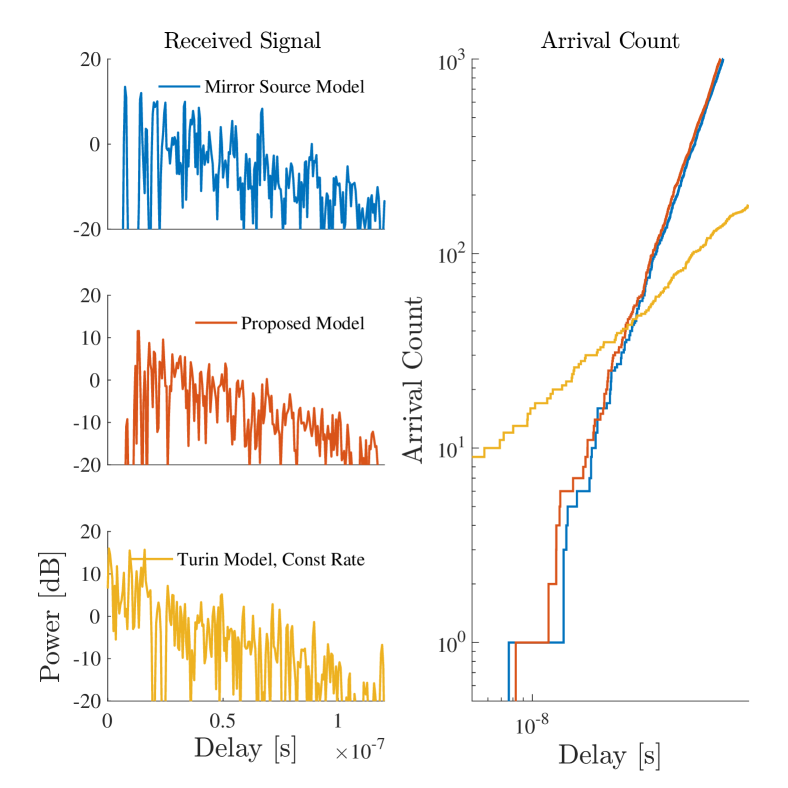
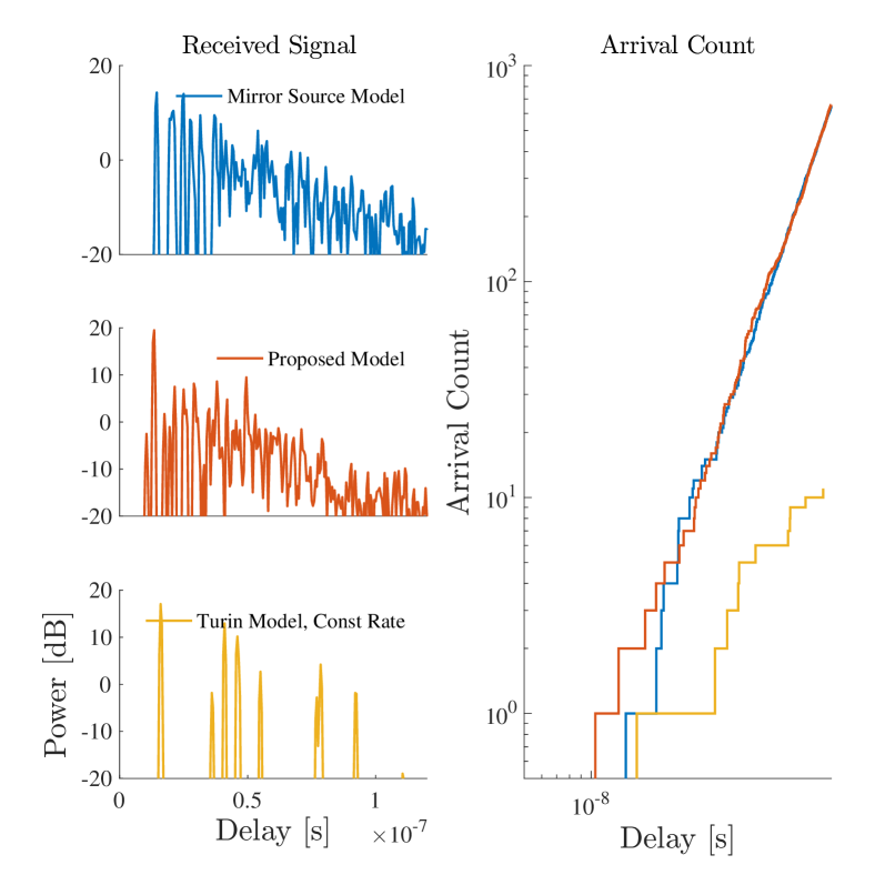
(a) Isotropic Antennas $\omega_{T}=\omega_{R}=1$	(b) Hemisphere Antennas $\omega_{T}=\omega_{R}=0.5$

Figure 2: Example realizations of the received signal (magnitude square) and corresponding arrival counts for (a) isotropic and (b) hemisphere antennas.

Fig. 2 gives examples of individual realizations for the squared magnitude of the received signal. The received signals for the mirror source model and the proposed approximation model both exhibit a specular to diffuse transition, i.e. early well separated specular components are succeeded by a gradually denser diffuse tail. This effect is not replicated by the constant rate model which is either “constantly sparse” or “constantly dense”.

Fig. 2 also show the arrival counts for the three models. The arrival counts are not observable in a measurement, but are easy to obtain in simulations. As expected, the arrival counts for the three models fluctuate about their respective theoretical mean count. The mirror source model and the proposed approximation produce similar realizations of arrival count versus delay while the constant rate model differ. Moreover, as predicted, the count for the isotropic antennas is four times higher than that obtained with the hemisphere antennas.

VI-B Power and Kurtosis of the Received Signal

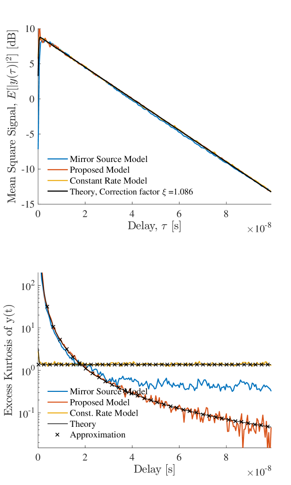
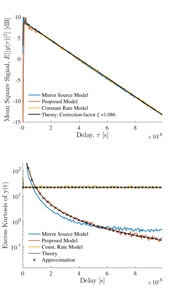
(a) Isotropic Antennas $\omega_{T}=\omega_{R}=1$	(b) Hemisphere Antennas $\omega_{T}=\omega_{R}=0.5$

Figure 3: Power and kurtosis of the received signal obtained from simulation, theory and approximation for (a) isotropic and (b) hemisphere antennas.

The upper panels of Fig. 3 shows the simulated expected received power versus delay for the three models along with the theoretical value computed using (10). The theoretical and simulated curves agree well for all three models with only minor deviations in the early parts of the spectra due to the applied Monte Carlo simulation technique. Thus, the simulations confirm that all three models have the same power delay spectrum and clearly exemplifies that models with very different arrival rates can indeed have identical second order statistics. Comparing the results for isotropic and hemisphere antennas it appears that the antenna directivity does not affect the power delay spectrum. In addition, we see that for the considered simulation setup, the high-bandwidth approximation obtained using (32) with $n=1$ is very accurate with some minor discrepancies at small delays.

Excess kurtosis delay spectra are reported in the lower panels of Fig. 3. The theoretical curves computed using (30) are close to to the large bandwidth approximations obtained using (32) and (33). The theory predicts the kurtosis to increase by a factor of four by replacing the isotropic antennas by hemisphere antennas. It appears that this shift is correctly represented in all three models. The simulations for the mirror source model agrees well with simulations of the proposed model. In particular this is true for the early part of the response which carries the most signal power. At later delays, however, the mirror source model deviates somewhat from the proposed. The deviation is caused in part by the small discrepancy in the model of the second moment, and in part due to the fact that the gain variables of the mirror source model is approximated by a Gaussian random variable. The discrepancy is furthermore accentuated by the logarithmic of the second axis. The curve for constant rate model clearly differs from the two others—as expected its kurtosis delay profile is constant. From this simulation it is apparent that models with identical delay power spectra may differ significantly in their predictions of the kurtosis delay spectrum.

VI-C Order Statistics of Arrival Times

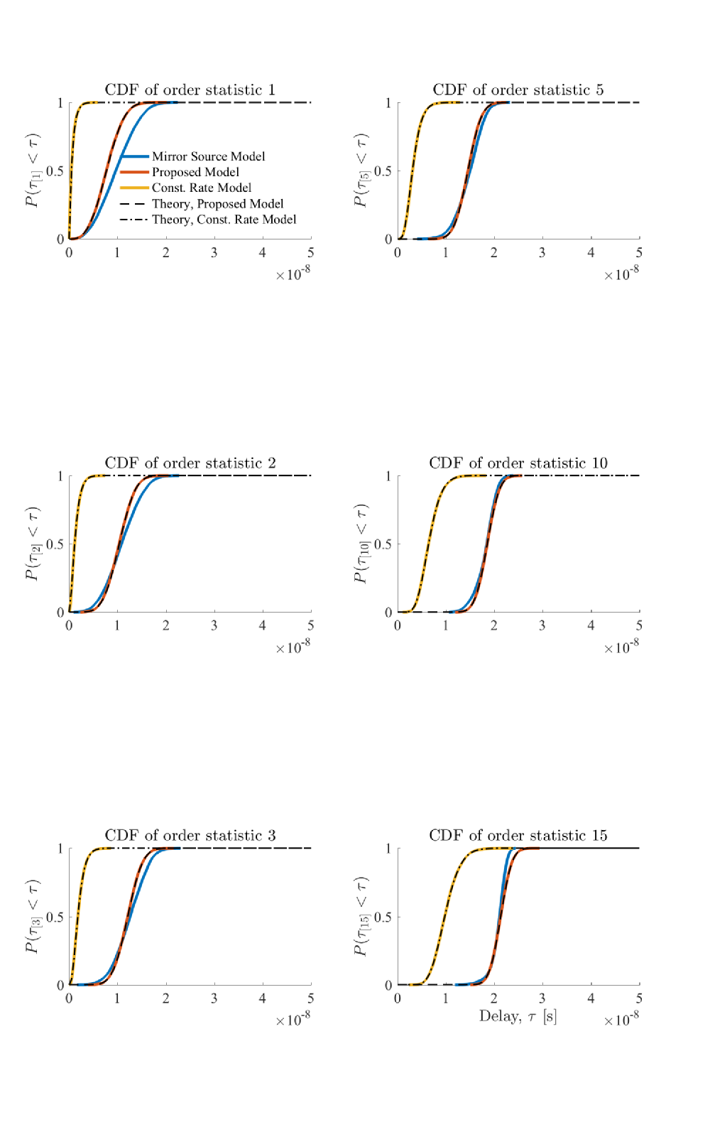
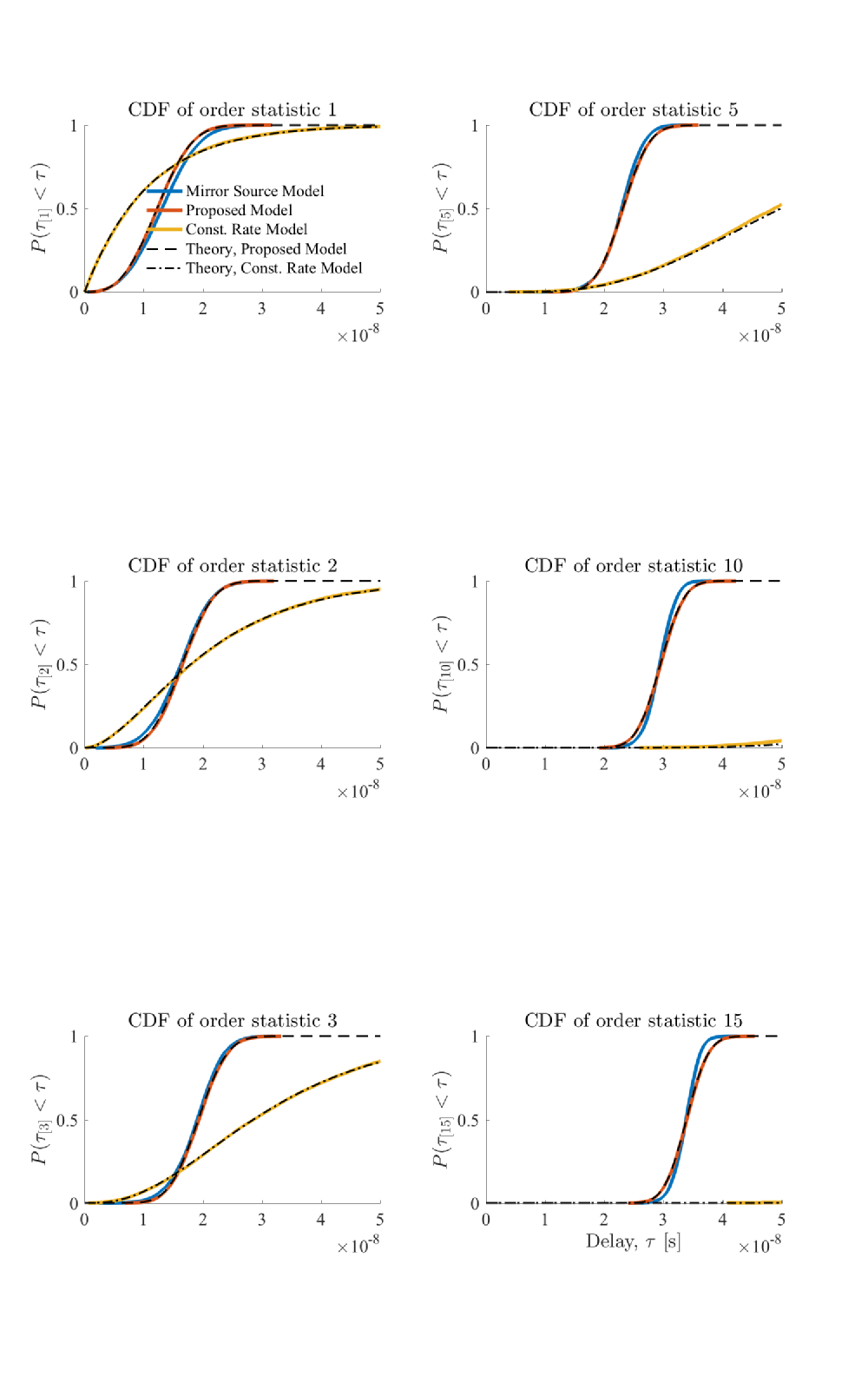
(a) Isotropic Antennas $\omega_{T}=\omega_{R}=1$	(b) Hemisphere Antennas $\omega_{T}=\omega_{R}=0.5$

Figure 4: Empirical cumulative probability for the order statistics of the three models with (a) isotropic and (b) hemisphere antennas. The theoretical cdfs given in dashed lines for the proposed and the constant rate models fall on top of the simulated curves.

The simulated order statistics for the arrival times reported in Fig. 4 give rise to a number of observations. As to be expected, for all models the cdfs of the order statistics move to the right as the order increases. Moreover, the slope of the cdf (related to the variance of the pdf) is steeper for the isotropic antennas than for the hemisphere antennas. This indicates that more directive antennas lead to a larger spread of the order statistics. For all considered order statistics, the proposed model captures more accurately the shape of the cdf than the constant rate model. This indicates that to accurately model the order statistics of the arrival process, it is important to model the arrival rate properly. In the considered case, the constant rate model is not appropriate. The deviations between the proposed model and the mirror source model are relatively minor and most significant in the first few order statistics and in the case with isotropic antennas. This effect shows that the approximation of the mirror source process in terms of Poisson process is most significant for isotropic antennas at the early delays, including the line-of-sight component.

VI-D Residual Power After Removing Paths

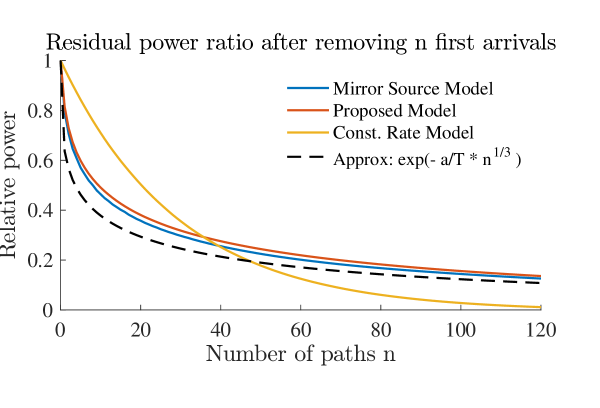
(a) Isotropic Antennas $\omega_{T}=\omega_{R}=1$

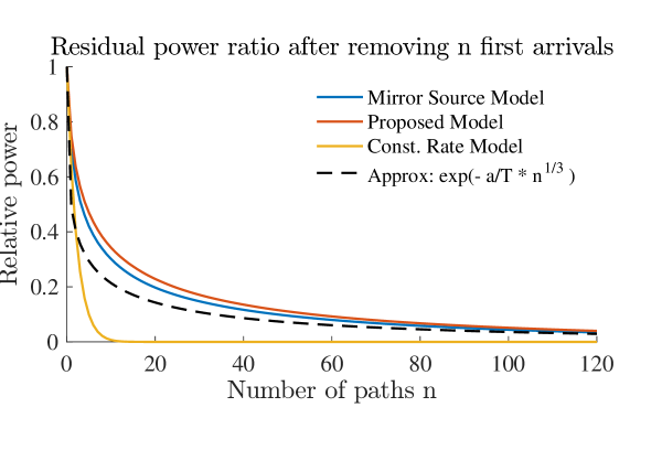
(b) Hemisphere Antennas $\omega_{T}=\omega_{R}=0.5$

Figure 5: The residual power relative to the total power for the three models after removing $n$ first paths for (a) isotropic and (b) hemisphere antennas. The approximation (47) is given in dashed line.

Fig. 5 shows the relative residual power after removing $n$ first arrivals. The residual power obtained with the proposed model fits well the results obtained from the mirror source model. This is to be expected in the light if the close match in order statistics observed in Fig. 4. Also, the approximation computed in (47) predicts well the trend of the received power. The constant rate model differ clearly from the two other models.

By comparing the upper and lower panels of Fig. 5 it is clear that the antenna characteristics affect the residual power for all three models. In the proposed model, the residual power depends only on the ratio $a/T$, it varies with room size, antenna characteristics, and the reverberation time. This observation is relevant in particular in connection with approximating the received signal using only a fixed number of multipath components such as commonly done using a high-resolution multipath estimators [39, 40, 41]. This model prediction is in agreement with the recently published measurement results [43] where the residual power after removing specular components is observed to decay at different rates for differently sized rooms.

VI-E Instantaneous Mean Delay and RMS Delay Spread

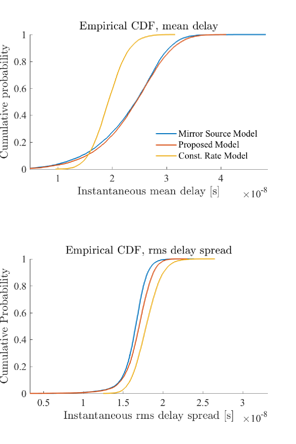
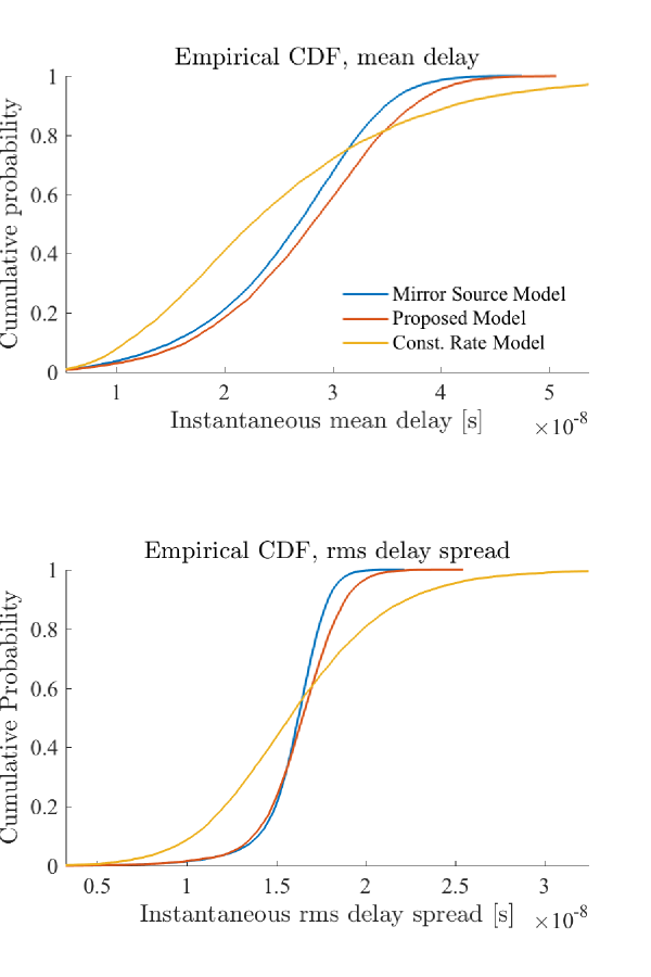
(a) Isotropic Antennas $\omega_{T}=\omega_{R}=1$		(b) Hemisphere Antennas $\omega_{T}=\omega_{R}=0.5$

Figure 6: Empirical cumulative probability for instantaneous mean delay and rms delay spread for (a) isotropic and (b) hemisphere antennas.

The distributions of instantaneous mean delay and rms delay spread are important for design of radio communication systems since numerous aspects of the system performance is characterized via these parameters. Therefore, we compare the considered models by comparing the resulting distribution of these parameters. Theoretical analysis of mean delay and rms delay spread is beyond the scope of this contribution, so we only report simulation results. Here, the mean and rms are computed as respectively the first and centered second temporal moments of each realizations of $|y(t)|^{2}$ (thus including the effect of the transmitted pulse).

The empirical cdfs for mean delay and rms delay spread reported in Fig. 6. It appears that proposed model is able to mimic the effects of the mirror source model well enough to accurately capture the distributions mean delay and rms delay spread. This is not the case for the constant rate model. All three models predict a shift of the curves as the directivity of the antennas change.

It should be noted that in the considered case, the three models have identical power delay spectra, and thus the differences between the proposed inhomogeneous and the constant models only stem from differences in higher moments which are controlled by their arrival rate. We conclude from these observations that accurate modeling of the arrival rate is a necessity to correctly model the distribution of instantaneous mean delay and rms delay spread.

VII Discussion

The proposed stochastic model is based on the mirror source analysis presented in [23]. Thus, the proposed model originates from an approximation of the mirror source theory for a very simplistic scenario where transmitter and receiver are placed in a rectangular room with perfectly flat walls void of other objects. Certainly, in most realistic scenarios, the walls will be imperfect due to doors, windows, heating devices, ventilation ducts, light fixtures and other such details. In addition, other objects in the room add to the complexity of the propagation environment. Therefore, the mirror source model should in itself be considered as an approximation of any real propagation environment.

We do expect, however, that since the very major elements of the inroom scenario, namely the walls, floor and ceiling are accounted for, the model can be used to qualitatively predict some effects that might occur in more realistic cases. We conjecture that if the scenario is made more complex, e.g by considering a furnished room, a number of mirror sources should be added which leads to an even faster growth of the arrival rate. This will speed up the diffusion process and result in an even faster decay of kurtosis delay profile.

The present contribution has focused on the theoretical analysis of the proposed model rather than its experimental validation. As discussed in [23], the power delay spectrum agrees with a model which has been previously been experimentally validated. Other predictions of the proposed approximation model have, however, not yet been compared to measurement data. We comment on validation of the model in the following.

The predictions related to the moments of the received signal can be validated as they are easy to relate to measurement data. In particular, the kurtosis delay profile could be estimated using using the estimator in Appendix B. While this seems straight-forward, we should bear in mind that reliable estimation of higher moments (here the fourth moment) usually calls for a large number of measurements. The presence of noise in the measurements may impair the estimation accuracy of especially the late part of the kurtosis delay profile. Therefore, we suggest that the robustness and noise-sensitivity of the estimator of the kurtosis delay profile should be investigated in more detail prior to applying these estimators.

To validate the model based on arrival delays and complex gains, (a part of) the marked point process $\mathcal{X}$ should be estimated. To this end, it is necessary to apply high-resolution estimators such as [39, 40, 41]. Such estimators, however, detect more easily multipath components with short delays which tend to have the strongest power and be better separated. Hence more signal components are missed by the estimator in the parts of the response where the density is the largest and the gains are the weakest. This effect can be considered as censoring of the observation [13] which may severely bias statistics based on estimates of arrival times.

As mentioned in Section V-B, it is a the widespread practice of calibrating and validating models for the arrival process by inspection of the empirical distribution of interarrival times. The interarrival times suffer from similar censoring problems as the arrival times. Moreover, due to the inhomogeneity of the proposed model, the interarrival times are not well defined. For these reasons we find the use of interarrival time statistics to be questionable. A more robust method could be to use the first few order statistics for calibration and validation since these are very likely to stem from strong and well separated signal components. In either case, when calibrating and validating multipath models based on estimation of arrival times, the properties and biases caused by the delay estimation procedure should be understood and factored in.

The model presented is constructed from physical analysis based on mirror source theory. This approach provides insight into how the environment (here the room) and the system parameters (here the antennas and the transmitted signal) affect the model. This insight is advantageous compared to an empirical model. Empirical models, however, can be more easily fitted to measurement data. It is therefore worth mentioning that the arrival rate model considered here may be also used to motivate an empirical model of the form

$$\lambda(\tau)=\eta\cdot\tau^{2}\cdot\mathds{1}(\tau>0),$$ (48)

where the factor $\eta$ should be determined from measurements. The complexity of this quadratic rate model is the same as the constant rate model, since either are defined by only a single parameter. The model 48 is able to represent the specular-to-diffuse transition observed experimentally for inroom channels. Such a transition effect is not captured by the constant rate model.

VIII Conclusion

We have proposed a stochastic model for the arrival times in an in-room scenario. The proposed model is based on approximation of the positions of mirror sources by spatial (3D) Poisson process. This induces a non-homogenous Poisson process for the arrival times and a model for the second moment of the power gain of a multipath component conditioned on its arrival time. By construction, the path arrival rate and power delay spectrum of the resulting stochastic multipath model agrees with the mirror source model. Nonetheless, the statistical structure of the mirror source process and thus of the arrival times, is not kept.

The proposed Poisson approximation is mathematically more convenient than the mirror source model as it enables closed-form derivation of expressions of a number of signal characteristics. Here we derive the cumulant generating functional for the received signal and use it to obtain the kurtosis delay spectrum of the received signal. The kurtosis depends on the arrival rate in a very direct fashion. In the high-bandwidth case, the arrival rate is inversely proportional to the arrival rate. Due to the increasing arrival rate, the pdf of the received signal depends on delay. At small delays the received signal can differ significantly from a Gaussian but as the delay increases, the pdf approaches a Gaussian. Furthermore, we show that the order statistics of the arrival times, i.e. the time of the $n$th arrival, follows a generalized gamma distribution with the parameters determined by antenna coverage fractions and the room volume. Based on the order statistics, we give a closed form expression for the relative residual power after removing the first $n$ arrivals. Monte Carlo simulations show that the proposed model agrees well to the mirror source model in terms of power delay spectrum, kurtosis, order statistics of arrival times, mean delay and rms delay spread.

The constant rate model, while having power delay spectrum identical to the two other models, the does not predict well any of the other studied characteristics (distributions of mean delay, rms delay spread and order statistics). Thus, accurate modelling the received signal using a stochastic multipath model necessitate accurate modelling of the arrival rate. The constant rate model as used in e.g. the Saleh-Valenzuela model is not able to predict these characteristics

Appendix A Generating Functionals

The characteristic functional for $y(t)$ evaluated for arbitrary probing function $\phi(t)$ is defined as [44, 34]

$$C[\phi] =\mathbb{E}\bigg{[}\exp\big{(}j\Re\int\phi(t)y(t)dt\big{)}\bigg{]}$$ (49)

where $\Re$ denotes the real part. The complex natural logarithm of the characteristic functional is the cumulant generating functional denoted by $K[\phi]$. By Kingmann’s marking theorem [32], the marked point process $\{(\tau_{\ell},\alpha_{\ell})\}$ with forms a two-dimensional Poisson process with rate $p(\alpha|\tau)\lambda(\tau)$. Then using Campbell’s theorem [32] and taking the logarithm we obtain

$$K[\phi] =\iint\big{(}e^{j\Re\alpha\int\phi(t)s(t-\tau)dt}-1\big{)}p(\alpha|\tau)\lambda(t)d\alpha d\tau$$ (50)

$$=\int\bigg{[}C_{\alpha|\tau}(\int\phi(t)s(t-\tau)dt)-1\bigg{]}\lambda(\tau)d\tau$$ (51)

where $C_{\alpha|\tau}(\cdot)$ is the characteristic function for $p(\alpha|\tau)$.

The probing function plays the same role as the variable introduced in the more widespread characteristic and cumulant generating functions. Evaluating the cumulant generating functional for $\phi(t)=\nu\delta(t)$, we obtain the cumulant generating function for $y(t)$ for any given time $t$:

$$K(\nu)=\int\bigg{[}C_{\alpha|\tau}(\nu s(t-\tau))-1\bigg{]}\lambda(\tau)d\tau$$ (52)

Cumulants of $y(t)$ can now be computed by complex differentiation as

$$\kappa_{m:n}(t) =\frac{\partial^{m+n}}{\partial^{m}\nu\partial{\nu^{*}}^{n}}K(\nu)\bigg{|}_{\nu=0}$$ (53)

$$=\int s(t-\tau)^{m}s(t-\tau)^{*n}\mathbb{E}[\alpha^{m}{\alpha^{*}}^{n}|\tau]\lambda(\tau)d\tau.$$ (54)

Considering the gains to be circular random variables, the moments $\mathbb{E}[\alpha^{m}{\alpha^{*}}^{n}|\tau]$ are zero for $m\neq n$ and all odd cumulants (and moments) of $y(t)$ vanish. The even cumulants in (27) are obtained with $m=n$. In particular for $m=n=1$ we obtain the delay power spectrum, i.e $\kappa_{1:1}(\tau)=P(\tau)$.

Appendix B Kurtosis Estimation for Complex Circular Variables

Here derive an estimator for the fourth cumulant of a circular complex random variable $X$ based iid. observations $X_{1},\dots,X_{N}$. For a circular complex variable, the fourth cumulant, fourth and second moments are related as [33]

$$\kappa_{2:2}[X]=\mathbb{E}[|X|^{4}]-2\mathbb{E}[|X|^{2}]^{2}.$$ (55)

We seek an estimator of the form

$$\hat{\kappa}_{2:2}[X]=c_{1}\sum_{n=1}^{N}{|X_{n}|^{4}}-c_{2}\left(\sum_{n=1}^{N}|X_{i}|^{2}\right)^{2}\!.$$ (56)

For an unbiased estimator, $\mathbb{E}[\hat{\kappa}_{2:2}[X]]=\kappa_{2:2}[X]$. By using (55) and some straight-forward manipulations we obtain

$$c_{1}=\frac{N+1}{N(N-1)},\quad\text{and }\quad c_{2}=\frac{2}{N(N-1)},\quad N>1.$$ (57)

Note this estimator differs from the unbiased estimator obtained for real valued data derived in [45]. The kurtosis is then estimated as $\hat{\kappa}_{2:2}[X]/\hat{\kappa}_{1:1}^{2}[X]$.

Appendix C Simulation of Inhomogeneous Poisson Process

The inhomogeneous Poisson point process $\mathcal{T}_{\mathrm{PPP}}$ can be simulated on a finite interval $[0,\tau_{\max}]$ by a two-step procedure: 1) Draw a Poisson count $N(\tau_{\mathrm{max}})$ with mean $\mathbb{E}[N(\tau_{\max})]$ as specified by the model. 2) Draw $N(\tau_{\mathrm{max}})$ iid. delay variables according to the pdf in (39). The corresponding cdf

$$F(\tau)=\begin{cases}0&\tau<0\\ \frac{\tau^{3}}{\tau_{\max}^{3}}&0\leq\tau\leq\tau_{\max}\\ 1&\tau<\tau_{\max}.\end{cases}$$ (58)

is easy to invert, and therefore we can use the inverse cumulative distribution method [35]. This amounts to transforming a variable $U$ uniformly distributed on the interval $[0,1]$ according to $\sqrt[3]{U}\tau_{\max}$.

References

- [1] G. Turin, F. Clapp, T. Johnston, S. Fine, and D. Lavry, “A statistical model of urban multipath propagation channel,” IEEE Trans. Veh. Technol., vol. 21, pp. 1–9, Feb. 1972.
- [2] H. Suzuki, “A statistical model for urban radio propagtion channel,” IEEE Trans. on Commun. Syst., vol. 25, pp. 673–680, Jul. 1977.
- [3] H. Hashemi, “Simulation of the urban radio propagation,” IEEE Trans. Veh. Technol., vol. 28, pp. 213–225, Aug. 1979.
- [4] A. A. M. Saleh and R. A. Valenzuela, “A statistical model for indoor multipath propagation channel,” IEEE J. Sel. Areas Commun., vol. SAC-5, no. 2, pp. 128–137, Feb. 1987.
- [5] Q. H. Spencer, B. Jeffs, M. Jensen, and A. Swindlehurst, “Modeling the statistical time and angle of arrival characteristics of an indoor multipath channel,” IEEE J. Sel. Areas Commun., vol. 18, no. 3, pp. 347–360, 2000.
- [6] T. Zwick, C. Fischer, and W. Wiesbeck, “A stochastic multipath channel model including path directions for indoor environments,” IEEE J. Sel. Areas Commun., vol. 20, no. 6, pp. 1178–1192, Aug. 2002.
- [7] T. Zwick, C. Fischer, D. Didascalou, and W. Wiesbeck, “A stochastic spatial channel model based on wave-propagation modeling,” IEEE J. Sel. Areas Commun., vol. 18, no. 1, pp. 6–15, Jan. 2000.
- [8] C.-C. Chong and S. K. Yong, “A generic statistical-based UWB channel model for high-rise apartments,” IEEE Trans. Antennas Propag., vol. 53, no. 8, pp. 2389–2399, Aug. 2005.
- [9] A. Molisch, D. Cassioli, C.-C. Chong, S. Emami, A. Fort, B. Kannan, J. Karedal, J. Kunisch, H. Schantz, K. Siwiak, and M. Win, “A comprehensive standardized model for ultrawideband propagation channels,” IEEE Transactions on Antennas and Propagation, vol. 54, no. 11, pp. 3151–3166, nov 2006. [Online]. Available: http://dx.doi.org/10.1109/tap.2006.883983
- [10] C. Gustafson, K. Haneda, S. Wyne, and F. Tufvesson, “On mm-wave multipath clustering and channel modeling,” IEEE Trans. Antennas Propag., vol. 62, no. 3, pp. 1445–1455, Mar. 2014. [Online]. Available: http://dx.doi.org/10.1109/TAP.2013.2295836
- [11] K. Haneda, J. Jarvelainen, A. Karttunen, M. Kyro, and J. Putkonen, “A statistical spatio-temporal radio channel model for large indoor environments at 60 and 70 GHz,” IEEE Trans. Antennas Propag., vol. 63, no. 6, pp. 2694–2704, Jun. 2015. [Online]. Available: http://dx.doi.org/10.1109/tap.2015.2412147
- [12] M. K. Samimi and T. S. Rappaport, “3-D millimeter-wave statistical channel model for 5G wireless system design,” IEEE Trans on Microw. Theory and Techniques, vol. 64, no. 7, pp. 2207–2225, Jul. 2016. [Online]. Available: http://dx.doi.org/10.1109/TMTT.2016.2574851
- [13] A. Karttunen, C. Gustafson, A. F. Molisch, J. Järveläinen, and K. Haneda, “Censored multipath component cross-polarization ratio modeling,” IEEE Wireless Communications Letters, vol. 6, no. 1, pp. 82–85, Feb 2017.
- [14] A. Meijerink and A. F. Molisch, “On the physical interpretation of the Saleh–Valenzuela model and the definition of its power delay profiles,” IEEE Trans. Antennas Propag., vol. 62, no. 9, pp. 4780–4793, Sep. 2014.
- [15] C. Holloway, M. Cotton, and P. McKenna, “A model for predicting the power delay profile characteristics inside a room,” IEEE Trans. Veh. Technol., vol. 48, no. 4, pp. 1110–1120, July 1999.
- [16] J. Kunisch and J. Pamp, “An ultra-wideband space-variant multipath indoor radio channel model,” in IEEE Conf. on Ultra Wideband Systems and Technologies, 2003, Nov. 2003, pp. 290–294.
- [17] ——, “Measurement results and modeling aspects for the UWB radio channel,” in IEEE Conf. on Ultra Wideband Systems and Technologies, 2002. Digest of Papers, May 2002, pp. 19–24.
- [18] G. Steinböck, M. Gan, P. Meissner, E. Leitinger, K. Witrisal, T. Zemen, and T. Pedersen, “Hybrid model for reverberant indoor radio channels using rays and graphs,” IEEE Trans. Antennas Propag., vol. 64, no. 9, pp. 4036–4048, Sep. 2016. [Online]. Available: http://dx.doi.org/10.1109/tap.2016.2589958
- [19] G. Steinböck, T. Pedersen, B. Fleury, W. Wang, and R. Raulefs, “Calibration of the Propagation Graph Model in Reverberant Rooms,” in URSI Commission F Triennial Open Symposium on Radiowave Propagation and Remote Sensing, May 2013.
- [20] T. Pedersen and B. H. Fleury, “A realistic radio channel model based on stochastic propagation graphs,” in Proceedings 5th MATHMOD Vienna – 5th Vienna Symposium on Mathematical Modelling, vol. 1,2, Feb. 2006, p. 324, ISBN 3–901608–30–3.
- [21] T. Pedersen and B. Fleury, “Radio channel modelling using stochastic propagation graphs,” in Proc. IEEE International Conf. on Commun. ICC ’07, Jun. 2007, pp. 2733–2738.
- [22] T. Pedersen, G. Steinböck, and B. H. Fleury, “Modeling of reverberant radio channels using propagation graphs,” IEEE Trans. Antennas Propag., vol. 60, no. 12, pp. 5978–5988, Dec. 2012.
- [23] T. Pedersen, “Modelling of path arrival rate for in-room radio channels with directive antennas,” submitted to IEEE Trans. Antennas and Propagation, 2017.
- [24] M. L. Jakobsen, B. H. Fleury, and T. Pedersen, “Analysis of the stochastic channel model by Saleh & Valenzuela via the theory of point processes,” in Int. Zurich Seminar on Communications (IZS), February 29 - March 2, 2012. Zürich, Eidgenössische Technische Hochschule Zürich, 2012. [Online]. Available: https://doi.org/10.3929/ethz-a-007052489
- [25] C. F. Eyring, “Reverberation time in ’dead’ rooms,” The Journal of the Acoustical Society of Amarica, vol. 1, no. 2, p. 241, 1930.
- [26] G. Steinböck, T. Pedersen, B. H. Fleury, W. Wang, and R. Raulefs, “Experimental validation of the reverberation effect in room electromagnetics,” IEEE Trans. Antennas Propag., vol. 63, no. 5, pp. 2041–2053, May 2015. [Online]. Available: http://dx.doi.org/10.1109/TAP.2015.2423636
- [27] H. Kuttruff, Room Acoustics. London: Taylor & Francis, 2000.
- [28] G. Steinböck, T. Pedersen, B. H. Fleury, W. Wang, and R. Raulefs, “Distance dependent model for the delay power spectrum of in-room radio channels,” IEEE Trans. Antennas Propag., vol. 61, no. 8, pp. 4327–4340, Aug. 2013. [Online]. Available: http://dx.doi.org/10.1109/tap.2013.2260513
- [29] M. G. Kendall and P. A. P. Moran, Geometrical Probability. London: Charles Griffin and Company Limited, 1963.
- [30] N. Minami, “On the poisson limit theorems of Sinai and Major,” Communications in Mathematical Physics, vol. 213, no. 1, pp. 203–247, 2000. [Online]. Available: http://dx.doi.org/10.1007/s002200000236
- [31] J. Bourgain, P. Sarnak, and Z. Rudnick, Modern Trends in Constructive Function Theory. American Mathematical Society (AMS), 2016, ch. Local Statistics of Lattice Points on the Sphere, pp. 269–282. [Online]. Available: http://dx.doi.org/10.1090/conm/661/13287
- [32] J. F. C. Kingman, Poisson Processes. Oxford University Press, 1993.
- [33] P. J. Schreier and L. L. Scharf, Statistical Signal Processing of Complex-Valued Data. Cambridge University Press, 2010.
- [34] D. L. Snyder and M. Miller, Random Point Processes in Time and Space. Springer-Springer-Verlag, Inc., 1991.
- [35] A. C. Davison, Statistical Models. Cambridge University Press, 2003.
- [36] G. B. Arfken and H. J. Weber, Mathematical Methods for Physicists, 5th ed. Hartcourt/Academic Press, 2001.
- [37] E. W. Stacy, “A generalization of the gamma distribution,” The Annals of Mathematical Statistics, vol. 33, no. 3, pp. 1187–1192, 1962. [Online]. Available: http://www.jstor.org/stable/2237889
- [38] S. Nadarajah and S. Kotz, “Comments on "a generic statistical-based uwb channel model for high-rise apartments,” IEEE Trans. Antennas Propag., vol. 56, no. 6, pp. 1831–1831, June 2008.
- [39] J. A. Högbom, “Aperture synthesis with a non-regular distribution of interferometer baselines,” Astronomy and Astrophysics Supplement Series, vol. 15, no. 3, pp. 417–426, 1974.
- [40] B. H. Fleury, M. Tschudin, R. Heddergott, D. Dahlhaus, and K. L. Pedersen, “Channel parameter estimation in mobile radio environments using the SAGE algorithm,” IEEE J. Sel. Areas Commun., vol. 17, no. 3, pp. 434–450, Mar. 1999.
- [41] R. Thomä, M. Landmann, G. Sommerkorn, and A. Richter, “Multidimensional high-resolution channel sounding in mobile radio,” in Proc. 21st IEEE Instrumentation and Measurement Technology Conf., IMTC, vol. 1, May 2004, pp. 257–262.
- [42] F. W. Olver, D. W. Lozier, R. F. Boisvert, and C. W. Clark, Eds., NIST Handbook of Mathematical Functions. Cambridge University Press, 2010.
- [43] K. Saito, J. I. Takada, and M. Kim, “Dense multipath component characteristics in 11-GHz-band indoor environments,” IEEE Trans. Antennas Propag., vol. 65, no. 9, pp. 4780–4789, Sept 2017.
- [44] J. Rice, “On generalized shot noise,” Advances in Applied Probability, vol. 9, no. 3, p. 553, Sep. 1977. [Online]. Available: http://dx.doi.org/10.2307/1426114
- [45] I. V. Blagouchine and E. Moreau, “Unbiased adaptive estimations of the fourth-order cumulant for real random zero-mean signal,” IEEE Trans. Signal Process., vol. 57, no. 9, pp. 3330–3346, Sep. 2009.