Nonlinear stationary subdivision schemes
that reproduce trigonometric functions

Abstract.

In this paper we define a family of nonlinear, stationary, interpolatory subdivision schemes with the capability of reproducing conic shapes including polynomials upto second order. Linear, non-stationary, subdivision schemes do also achieve this goal, but different conic sections require different refinement rules to guarantee exact reproduction. On the other hand, with our construction, exact reproduction of different conic shapes can be achieved using exactly the same nonlinear scheme. Convergence, stability, approximation and shape preservation properties of the new schemes are analyzed. In addition, the conditions to obtain $\mathcal{C}^{1}$ limit functions are also studied.

Keywords. nonlinear subdivision schemes, exponential polynomials, reproduction, monotonicity preservation, approximation, smoothness.

MSC. 41A25, 41A30, 65D15, 65D17.

1. Introduction

Subdivision refinement is a powerful technique for the design and representation of curves and surfaces. Subdivision algorithms are simple to implement and extremely well suited for computer applications, which make them very attractive to users interested in geometric modeling and Computer Aided Geometric Design (CAGD).

As in [11, 12, 13], in this paper we consider that a subdivision scheme $S=(S^{k})_{k=0}^{\infty}$ is a sequence of operators $S^{k}:l_{\infty}(\mathds{Z})\longrightarrow l_{\infty}(\mathds{Z})$ such that for each $f^{0}\in l_{\infty}(\mathds{Z})$, a sequence $(f^{k})_{k=0}^{\infty}\subset l_{\infty}(\mathds{Z})$ is recursively defined as follows:

$$f^{k+1}:=S^{k}f^{k}\in l_{\infty}(\mathds{Z}),\quad k\geq 0.$$

We shall restrict our attention to binary subdivision schemes which are uniform and local, i.e. there exists $q\geq 0$ such that for any $f\in l_{\infty}(\mathds{Z})$

(1) $$(S^{k}f)_{2i+j}=\Psi_{j}^{k}(f_{i-q},\ldots,f_{i+q}),\qquad j=0,1,\quad{i\in\mathds{Z}},$$

for some $\Psi_{j}^{k}:\mathds{R}^{2q+1}\longrightarrow\mathds{R}$. If the functions $\Psi_{j}^{k}$ are linear, the level dependent rules can be expressed as follows

(2) $$\Psi_{j}^{k}(f_{i-q},\ldots,f_{i+q})=\sum_{l=-q}^{q}a_{j-2l}^{k}f_{i+l}\qquad{i\in\mathds{Z}},$$

where the sequence $(a^{k}_{i})_{i\in\mathds{Z}}$ (that has finite support) is the mask of the linear operator $S^{k}$, and the scheme is called linear. If the rules are the same at all refinement levels $k\geq 0$, then the scheme is said to be stationary, and we simply denote $S^{k}=S$, $\Psi^{k}_{j}=\Psi_{j}$ and $a^{k}_{i}=a_{i}$, $\forall k\geq 0$. The data generated by binary subdivision schemes are usually associated to the underlying grids ${2^{-k}\mathds{Z}}$, $k\geq 0$.

Subdivision schemes of interest in practical applications need to be convergent. In this paper, we are concerned with the classical notion of uniform convergence, which is relevant in geometric modeling.

Definition 1.

A binary subdivision scheme, $S$, is uniformly convergent if

(3) $$\forall f^{0}\in l_{\infty}(\mathds{Z})\quad\exists S^{\infty}f^{0}\in\mathcal{C}(\mathds{R})\,:\,\lim_{k\rightarrow\infty}\sup_{i\in\mathds{Z}}|f^{k}_{i}-(S^{\infty}f^{0})(i2^{-k})|=0.$$

If $S$ is a convergent subdivision scheme, $S^{\infty}:l_{\infty}(\mathds{Z})\rightarrow\mathcal{C}(\mathds{R})$ denotes the operator that sends any initial data $f^{0}$ to the continuous limit function obtained by the subdivision process specified by $S$. A uniformly convergent subdivision scheme is $\mathcal{C}^{m}$, or $\mathcal{C}^{m}$-convergent, if for any initial data the limit function has continuous derivatives up to order $m$.

Interpolatory subdivision refinement is often used in practical applications. Binary interpolatory subdivision schemes satisfy

(4) $$f^{k+1}_{2i}=(S^{k}f^{k})_{2i}=f^{k}_{i},\qquad\forall{i\in\mathds{Z}}.$$

Hence, they are defined by specifying only the so-called insertion rules, $\Psi^{k}_{1}$, that define $f^{k+1}_{2i+1}$ in (1). If $S$ is interpolatory and convergent then

(5) $$(S^{\infty}f^{0})(i2^{-k})=f_{i}^{k},$$

that is, $S^{\infty}f^{0}$ interpolates the data, $f^{k}$, at each resolution level. This property may be very useful in CAGD, where interpolatory subdivision schemes are often used to obtain specific shapes from an initial (coarse) set of samples.

One important property of linear non-stationary subdivision schemes, which linear stationary subdivision schemes do not have, is that they can be used to efficiently generate conical shapes (circles, ellipses…) from a coarse initial set of samples. For example, an initial representation of $n$ equidistant points on the unit circle is obtained by considering $f^{0}=(G(i))_{i\in\mathds{Z}}$ where $G(t)=(\cos(\gamma t),\sin(\gamma t))$, with $\gamma=2\pi/n$. From this initial coarse representation, the circle can be obtained by using interpolatory subdivision schemes capable of reproducing the trigonometric functions The relevant definition on function reproduction is provided below for completeness.

Definition 2.

A convergent subdivision scheme $S$ reproduces the set of continuous functions $\mathcal{V}$ if

(6) $$f^{0}_{i}=F(i)\quad\forall{i\in\mathds{Z}}\quad\Longrightarrow\quad S^{\infty}f^{0}=F,\qquad\forall F\in\mathcal{V}.$$

This paper is concerned with the efficient reproduction of conical sections by means of interpolatory stationary nonlinear subdivision schemes. In particular, we consider the (finite dimensional) spaces

(7) $$W_{0,\gamma}=\text{span}\left\{1,\exp(\gamma t),\exp(-\gamma t)\right\},\qquad 0\neq\gamma\in\mathbb{R}\cup\imath(-\pi,\pi),\qquad\imath=\sqrt{-1},$$

which can be used to represent circles, ellipses and hyperbolic functions centered anywhere in the plane.

As mentioned before, any linear scheme reproducing functions in this space must be necessarily non-stationary. In addition, the value of $\gamma$ must be known in order to determine the level-dependent rules of the non-stationary scheme (see e.g. [6, 13] and section 4). In practice, this value is estimated from the samples [13], but the dependence of these subdivision schemes on the value of the parameter $\gamma$ may be seen as a drawback when we desire to obtain shapes composed of different conical sections. In this case, several values of the parameter $\gamma$ might have to be estimated from the initial samples, and different schemes would have to be used for exact reproduction of the different sections. There is nowadays a relatively large body of research concerning linear, non-stationary subdivision schemes and their properties (see e.g. [6, 11, 13] and references therein).

In this paper, we shall construct and analyze a family of interpolatory, nonlinear, stationary subdivision schemes with the capability to reproduce $\Pi_{2}\cup W_{0,\gamma}$ for all $\gamma\in\mathds{R}\cup\imath[-\frac{3}{4}\pi,\frac{3}{4}\pi]$, independently of the value of $\gamma$, under rather general conditions. Hence, our schemes provide a simple and effective way to obtain curves composed of different conic/hyperbolic sections by recursive subdivision, obtaining exact reproduction in each of the conic sections.

The derivation of the nonlinear schemes proposed in this paper is based on the orthogonal rules that annihilate the space $W_{0,\gamma}$. Orthogonal rules are one possible way to derive non-stationary subdivision schemes capable of reproducing spaces of exponential polynomials (see [13] or section 3).

The paper is organized as follows: In sections 2 and 3 we recall the basic results about convergence of stationary subdivision schemes, both linear and nonlinear, as well as the essential ingredients on the spaces of exponential polynomials and the derivation of the orthogonal rules that are relevant in our construction. Sections 4 and 5 are dedicated to the definition and convergence analysis of the proposed nonlinear subdivision schemes. The preservation of monotonicity is analyzed in section 6. In section 7 we perform a study of the regularity of the limit functions obtained from monotone initial data, following (loosely) some ideas in [17]. The approximation capabilities and the stability are treated in section 8. Section 9 shows some numerical experiments that fully support our theoretical results. We close in section 10 with some conclusions ans future perspectives.

2. Convergence of stationary subdivision schemes.

In what follows, we set the notation for the remainder of the paper and briefly review those tools used in the analysis of stationary subdivision schemes (linear or not) that are relevant in our development. The interested reader is referred to [4, 12] for a more complete description of the theory of linear subdivision schemes, and to [2, 3, 8, 9, 16] for the relevant theory of nonlinear subdivision schemes that can be written as a nonlinear perturbation of a convergent linear scheme. In the following we use the letter $T$ only for linear schemes, while $S$ shall denote a general subdivision scheme (linear or not).

A well-known necessary condition for the convergence of a stationary subdivision scheme is that

(8) $$\sum_{i\in\mathds{Z}}a_{2i}=\sum_{i\in\mathds{Z}}a_{2i+1}=1.$$

The last relation is equivalent to the reproduction of constant sequences property and implies the existence of the first difference scheme $T^{[1]}$, characterized by the following property

$$\nabla Tf=T^{[1]}\nabla f,\qquad\forall f\,\in l_{\infty}(\mathds{Z}),$$

where $\nabla f=(f_{i+1}-f_{i})_{i\in\mathds{Z}}$. Moreover, if $T$ is a linear subdivision scheme satisfying (8), then $T$ is convergent if, and only if,

(9) $$\exists L>0,\eta<1:\quad\left\|(T^{[1]}\circ T^{[1]}\circ\overset{(L)}{\cdots}\circ T^{[1]})f\right\|_{\infty}\leq\eta\left\|f\right\|_{\infty}\quad\forall f\in l_{\infty}(\mathds{Z}).$$

In [1, 2, 3, 7, 8, 9, 16], the authors construct and analyze several nonlinear subdivision schemes that can be described as a (rather specific) nonlinear perturbation of a convergent linear scheme. In this paper, we are interested in subdivision schemes of the form

(10) $$Sf=Tf+\mathcal{F}(\nabla f),\qquad\forall f\in l_{\infty}(\mathds{Z}),$$

where $\mathcal{F}:l_{\infty}(\mathds{Z})\rightarrow l_{\infty}(\mathds{Z})$ may be a nonlinear operator and $T$ is a linear and convergent subdivision scheme (so $T^{[1]}$ exists). It is easy to see that schemes of the form specified in (10) always admit a first-difference scheme. Indeed, applying the difference operator, $\nabla$ to (10) we get

$$\nabla Sf=\nabla Tf+\nabla\mathcal{F}(\nabla f)=T^{[1]}\nabla f+\nabla\mathcal{F}(\nabla f).$$

Hence, $S^{[1]}$ is defined as

(11) $$S^{[1]}f=T^{[1]}f+\nabla\mathcal{F}(f),\qquad\forall f\in l_{\infty}(\mathds{Z}).$$

Then, convergence can be proven using the following result from [3] (notice the similarity with (9)).

Theorem 3.

Let $S$ be an interpolatory subdivision scheme of the form (10). If

(12) C1. $$\qquad\exists M>0: ||\mathcal{F}(f)||_{\infty}\leq M\left\|f\right\|_{\infty}, \forall f\in l_{\infty}(\mathds{Z}),$$

C2. $$\qquad\exists L>0,\,\,0<\eta<1: \left\|(S^{[1]}\circ S^{[1]}\circ\overset{L}{\cdots}\circ S^{[1]})(f)\right\|_{\infty}\leq\eta\left\|f\right\|_{\infty}, \forall f\in l_{\infty}(\mathds{Z}),$$

then $S$ is convergent. If $T$ is $\mathcal{C}^{\alpha}$, then $S$ is $\mathcal{C}^{\beta}$ with $\beta=\min\{\alpha,-\log_{2}(\eta)/L\}$.

Remark 4.

We write $F\in\mathcal{C}^{\alpha}$, being $\alpha=n+\kappa$, with $n\in\mathds{N}$ and $0<\kappa<1$, if $F^{(n)}$ exists and satisfies

$$|F^{(n)}(x)-F^{(n)}(y)|\leq C|x-y|^{\kappa}.$$

$S$ is $\mathcal{C}^{\alpha}$ if $S^{\infty}f^{0}\in\mathcal{C}^{\alpha}$ for any $f^{0}\in l_{\infty}(\mathds{Z})$. $S$ is $\mathcal{C}^{\alpha-}$ if $S$ is $\mathcal{C}^{\alpha-\theta}$ for any $\theta>0$ small enough.

In fact, it turns out that the regularity of $T$ in Theorem 3 does not limit the regularity of $S$.

Corollary 5.

Suppose that $S$ is interpolatory, of the form (10), and satisfies C1, C2 in Theorem 3. Then $S$ is $\mathcal{C}^{\beta}$ with $\beta=-\log_{2}(\eta)/L$.

Proof.

If $S$ is of the form (10), $S^{[1]}$ is well defined. Notice that the expression for $S^{[1]}$ in (11), together with the fact that $\mathcal{F}$ satisfies property C1 in Theorem 3, implies that there exists $C_{S}>0$ such that $\left\|S^{[1]}(f)\right\|_{\infty}\leq C_{S}\left\|f\right\|_{\infty}$.

Using $S^{[1]}$ we can write

$$(Sf)_{2i+1} =(Sf)_{2i+1}-(Sf)_{2i}+(Sf)_{2i}=\nabla(Sf)_{2i}+f_{i}=(S^{[1]}\nabla f)_{2i}+f_{i}$$

$$(Sf)_{2i+1} =(Sf)_{2i+2}-(Sf)_{2i+2}+(Sf)_{2i+1}=f_{i+1}-\nabla(Sf)_{2i+1}=f_{i+1}-(S^{[1]}\nabla f)_{2i+1}$$

$$(Sf)_{2i+1} =\frac{1}{2}((S^{[1]}\nabla f)_{2i}+f_{i})+\frac{1}{2}(f_{i+1}-(S^{[1]}\nabla f)_{2i+1})=\frac{1}{2}f_{i}+\frac{1}{2}f_{i+1}-\frac{1}{2}((S^{[1]}\nabla f)_{2i+1}-(S^{[1]}\nabla f)_{2i}).$$

Hence, we can write

$$Sf=T_{1,1}f+\mathcal{F}_{S}(\nabla f),\qquad\mathcal{F}_{S}(f)_{2i+1}=-\frac{1}{2}((S^{[1]}f)_{2i+1}-(S^{[1]}f)_{2i}),$$

where $T_{1,1}$ denotes the 2-point Deslauriers-Dubuc scheme.

By applying the same argument to $T_{n,n}$, the 2n-point Deslauriers-Dubuc interpolatory subdivision scheme, we can also write

$$T_{n,n}=T_{1,1}+\mathcal{F}_{n,n}(\nabla f).$$

Thus, we have too

$$Sf=T_{n,n}f+(\mathcal{F}_{S}-\mathcal{F}_{n,n})(\nabla f).$$

Notice that $S^{[1]}$ and $T_{n,n}$ are bounded operators, hence $\mathcal{F}_{S}$ and $\mathcal{F}_{n,n}$ and $\mathcal{F}_{S}-\mathcal{F}_{n,n}$ satisfy condition ${C1}$ in Theorem 3.

Since $S$ satisfies condition C2, its regularity is $\mathcal{C}^{\beta}$, $\beta=\min\{-\frac{\log_{2}(\eta)}{L},\alpha_{n}\}$, where $\alpha_{n}$ is the regularity of $T_{n,n}$. But $n$ was taken arbitrarily and $\alpha_{n}\overset{n\rightarrow\infty}{\longrightarrow}+\infty$ (see e.g. [10]), then $\beta=-\frac{\log_{2}(\eta)}{L}$. ∎

3. Linear subdivision schemes that reproduce Exponential Polynomials. Orthogonal Rules

The reproduction of certain finite dimensional spaces is always an important issue in subdivision refinement. In particular, for linear interpolatory subdivision schemes there is a well known relation between the smoothness of the scheme and the reproduction of spaces of polynomials [12].

Conic sections, spirals and other objects of interest in geometric modeling can be expressed as combinations of exponential polynomials. The reproduction of such (finite-dimensional) spaces, a very desirable property in CAGD, has been thoroughly studied in the literature. The study of non-stationary subdivision schemes reproducing general spaces of exponential polynomials was initiated in 2003 in [13]. We recall that these spaces are associated to the space of solutions of certain linear differential operator and refer the reader to [6, 13, 18] for further information. Here, we shall only recall the definitions and concepts relevant to our development.

General Exponential Polynomial (EP) spaces are defined in terms of two sets of parameters, $\bar{\gamma}=(\gamma_{0},\gamma_{1},\ldots,\gamma_{\nu})$, $\gamma_{i}\neq\gamma_{j}$, $i\neq j$, $\gamma_{i}\in\mathbb{C}$ and $\bar{\mu}=(\mu_{0},\mu_{1},\ldots,\mu_{\nu})$, $0\leq\mu_{i}\in\mathbb{N}$, for some fixed $\nu\in\mathds{N}$, $\nu\geq 0$. In this paper, the associated space of exponential polynomials shall be denoted as follows

(13) $$V_{\bar{\gamma}}^{\bar{\mu}}=\text{span}\left\{t^{l}\exp(\gamma_{n}t):l=0,1,\ldots,\mu_{n}-1,\,n=0,1,\ldots,\nu\right\}.$$

Notice that $V^{(1,1,1)}_{(0,\gamma,-\gamma)}=W_{0,\gamma}$, a notation used mainly for simplicity throughout the paper.

We remark again that the set of parameters that define a particular EP space needs to be known in order to determine the linear, non-stationary, interpolatory subdivision scheme capable of reproducing the space. In practice, given an initial set of samples, the parameters that determine the correct refinement rules are determined by a preprocessing step [13].

As pointed out in [13] (Theorem 2.5), there exists a unique Minimal-Rank (M-R) reproducing subdivision scheme for a given EP space of the form (13). Its mask can be derived from a linear system of equations (Theorem 2.3 of [13]) or from the orthogonal rules of the EP space. These rules annihilate samples of any function in the desired given EP space and give rise to the so-called orthogonal schemes.

We recall next the definition of the Z-transform of a sequence $f=(f_{i})_{i\in\mathds{Z}}$ as the formal Laurent series

$$\mathcal{Z}\left(f,z\right)=\sum_{i\in\mathds{Z}}f_{i}z^{i}.$$

Note that $\mathcal{Z}\left(\cdot,z\right)$ is a linear operator and that $\mathcal{Z}\left(f,z\right)$ is a well-defined function for $z\in\mathds{C}$, $0<|z|<1$, if $f\in l_{\infty}(\mathds{Z})$. In terms of the Z-transform, (2) can be equivalently expressed as follows,

$$\mathcal{Z}\left(T^{k}f,z\right)=\mathcal{Z}\left(a^{k},z\right)\mathcal{Z}\left(f,z^{2}\right).$$

The Laurent polynomial $a^{k}(z):=\mathcal{Z}\left(a^{k},z\right)$ is the symbol of $T^{k}$.

Definition 6.

Orthogonal Rule. A Laurent series $b^{k}(z)=\sum_{i\in\mathds{Z}}b_{i}^{k}z^{i}$ is an orthogonal rule for the functional vector space $\mathcal{V}$ at ${2^{-k}\mathds{Z}}$ if

$$b^{k}(z)\mathcal{Z}\left(F^{k},z\right)=0,\qquad\forall F\in\mathcal{V},\quad F^{k}:=F|_{2^{-k}\mathds{Z}}.$$

One of the easiest examples of orthogonal rules is obtained from the fact that the $\mu$-th finite difference operator annihilates equal-spaced samples of $\Pi_{\mu-1}$, the space of polynomials of degree up to $\mu-1$. Using the Z-transform on the relation

$$\nabla^{\mu}P^{k}=0,\qquad\forall k\geq 0,\quad\forall P\in\Pi_{\mu-1}$$

we obtain

(14) $$z^{-\mu}(1-z)^{\mu}\mathcal{Z}\left(P^{k},z\right)=0.$$

hence $b(z)=(1-z)^{\mu}$ is an orthogonal rule for $\Pi_{\mu-1}$ for any $\mu\geq 1$. Using this result, we shall see next that we can easily obtain orthogonal rules to various EP spaces.

Theorem 7.

Let $\bar{\gamma}\in\mathds{C}^{\nu+1}$, $\bar{\mu}\in\mathds{N}^{\nu+1}$, with $\gamma_{i}\neq\gamma_{j}$ if $i\neq j$. Then

$$\left(\prod_{n=0}^{\nu}(1-\exp(2^{-k}\gamma_{n})z)^{\mu_{n}}\right)\mathcal{Z}\left(F^{k},z\right)=0,\quad\forall F\in V_{\bar{\gamma}}^{\bar{\mu}}.$$

Proof.

Consider first the case $\nu=0$, $\gamma_{0}=\gamma$, $\mu_{0}=\mu$. In this case, functions in $V_{\gamma}^{\mu}$ are of the form $F(t)=\exp(\gamma t)P(t)$, with $P(t)\in\Pi_{\mu-1}$. Then $F^{k}_{i}=\exp(2^{-k}i\gamma)P(2^{-k}i)$, and we have

$$\mathcal{Z}\left(F^{k},z\right)=\sum_{i\in\mathds{Z}}\exp(2^{-k}\gamma i)P(2^{-k}i)z^{i}=\sum_{i\in\mathds{Z}}P(2^{-k}i)(\exp(2^{-k}\gamma)z)^{i}=\mathcal{Z}\left(P^{k},\exp(2^{-k}\gamma)z\right),$$

with $P^{k}=(P(2^{-k}i))_{i\in\mathds{Z}}$. Replacing $z$ by $\exp(2^{-k}\gamma)z$ in (14) we obtain

$$0=(1-\exp(2^{-k}\gamma)z)^{\mu}\mathcal{Z}\left(P^{k},\exp(2^{-k}\gamma)z\right)=(1-\exp(2^{-k}\gamma)z)^{\mu}\mathcal{Z}\left(F^{k},z\right).$$

Now, for $\nu>0$, $F\in V_{\bar{\gamma}}^{\bar{\mu}}$ can be written as

$$F(t)=\sum_{n=0}^{\nu}F_{n}(t),\qquad F_{n}\in V_{\gamma_{n}}^{\mu_{n}}=\text{span}\left\{t^{l}\exp(\gamma_{n}t):l=0,\ldots,\mu_{n}-1\right\}.$$

Since (by the case $\nu=0$)

$$(1-\exp(2^{-k}\gamma_{n})z)^{\mu_{n}}\mathcal{Z}\left(F_{n}^{k},z\right)=0$$

we have

$$\left(\prod_{n=0}^{\nu}(1-\exp(2^{-k}\gamma_{n})z)^{\mu_{n}}\right)\mathcal{Z}\left(F_{m}^{k},z\right)=0,\qquad m=0,\ldots,\nu$$

hence

$$0=\left(\prod_{n=0}^{\nu}(1-\exp(2^{-k}\gamma_{n})z)^{\mu_{n}}\right)\sum_{m=0}^{\nu}\mathcal{Z}\left(F_{m}^{k},z\right)=\left(\prod_{m=0}^{\nu}(1-\exp(2^{-k}\gamma_{m})z)^{\mu_{m}}\right)\mathcal{Z}\left(F^{k},z\right).$$

∎

The next example shows how the orthogonal rules of an EP space can be used to define a linear, non-stationary, subdivision scheme reproducing the given EP space. It also serves to examine a relation between the non-stationary linear scheme obtained and a stationary nonlinear rule, that is essentially equivalent to the non-stationary refinement rules for data sampled in the given EP space. This derivation will be useful, in section 4, in the construction of our new family of subdivision schemes.

Example 8.

Circles, hyperbolas and ellipses, centered at the origin, can be drawn using functions in the EP space (for suitable values of the parameter $\gamma$)

$$V_{(\gamma,-\gamma)}^{(1,1)}:=\text{span}\left\{\exp{(\gamma t)},\exp{(-\gamma t)}\right\}.$$

Using Theorem 7, we obtain that $\forall F\in V_{(\gamma,-\gamma)}^{(1,1)}$

(15) $$0 =(1-\exp(2^{-k}\gamma)z)(1-\exp(-2^{-k}\gamma)z)\mathcal{Z}\left(F^{k},z\right)=(1-2\phi_{\gamma,k}z+z^{2})\mathcal{Z}\left(F^{k},z\right)$$

with

(16) $$\phi_{\gamma,k}:=\frac{1}{2}\left(\exp(2^{-k}\gamma)+\exp(-2^{-k}\gamma)\right)=\begin{cases}\cosh(2^{-k}|\gamma|),&\gamma\in\mathds{R}\\ \cos(2^{-k}|\gamma|),&\gamma\in\imath\mathds{R}.\end{cases}$$

Rewriting (15) as

(17) $$\sum_{i\in\mathds{Z}}\left(F_{i}^{k}-2\phi_{\gamma,k}F_{i-1}^{k}+F_{i-2}^{k}\right)z^{i}=0,$$

and considering the coefficients of the even powers in the Laurent series, we get

$$F_{2i+2}^{k}-2\phi_{\gamma,k}F_{2i+1}^{k}+F_{2i}^{k}=0,\qquad\forall{i\in\mathds{Z}}.$$

Then, since $F_{2i}^{k}=F_{i}^{k-1}$, we can write

(18) $$F_{2i+1}^{k}=\frac{1}{2\phi_{\gamma,k}}F_{i+1}^{k-1}+\frac{1}{2\phi_{\gamma,k}}F_{i}^{k-1}.$$

Thus, the linear, non-stationary, subdivision scheme

(19) $$f^{k+1}_{2i}=f^{k}_{i},\quad f^{k+1}_{2i+1}=\frac{1}{2\phi_{\gamma,k+1}}f^{k}_{i+1}+\frac{1}{2\phi_{\gamma,k+1}}f^{k}_{i}$$

reproduces $V_{(\gamma,-\gamma)}^{(1,1)}$, provided $\gamma$ is such that $\phi_{\gamma,k}\neq 0$, $\forall k\geq 1$. This condition is obviously fulfilled for any $\gamma\in\mathbb{R}$, and for $\gamma\in\imath(-\pi,\pi)$. Note that for $\gamma=0$ the scheme becomes

$$f^{k+1}_{2i}=f^{k}_{i},\quad f^{k+1}_{2i+1}=\frac{1}{2}f^{k}_{i+1}+\frac{1}{2}f^{k}_{i},$$

i.e. the 2-point Deslauriers-Dubuc, $T_{1,1}$, subdivision scheme (which reproduces $\Pi_{1}$).

Next, we derive a nonlinear stationary rule that is essentially equivalent to (18), in a sense to be made precise later. There are two key points in this derivation. The first one is that (17) implies that the parameters $\phi_{\gamma,k}$ can be obtained from the level-$k$ samples of functions $F\in V^{(1,1)}_{(\gamma,-\gamma)}$, provided that $F^{k}_{i}\neq 0$, as follows

(20) $$\phi_{\gamma,k}=\frac{F^{k}_{i-1}+F^{k}_{i+1}}{2F^{k}_{i}}.$$

The second key point is that the definition of $\phi_{\gamma,k}$ in (16) implies that the following two-scale relation holds true,

(21) $$\phi_{\gamma,k+1}^{2}=\frac{1}{2}(1+\phi_{\gamma,k}),\qquad\forall k\geq 0.$$

Assuming that $\imath\gamma\in(-\pi,\pi)$ or $\gamma\in\mathds{R}$, so that $\phi_{\gamma,k+1}>0$, from (21) and (20) we get

$$\phi_{\gamma,k+1}=\sqrt{\frac{1}{2}(1+\phi_{\gamma,k})}=\sqrt{\frac{F^{k}_{i-1}+2F^{k}_{i}+F^{k}_{i+1}}{4F^{k}_{i}}}.$$

Thus, from (18) and the expression above, we obtain the following nonlinear relation for the point-values of $F\in V_{(\gamma,-\gamma)}^{(1,1)}$ (under appropriate restrictions so that the operations involved may take place)

$$F^{k+1}_{2i+1}=\sqrt{\frac{F^{k}_{i}}{F^{k}_{i-1}+2F^{k}_{i}+F^{k}_{i+1}}}(F_{i}^{k}+F_{i+1}^{k}),\qquad F\in V_{(\gamma,-\gamma)}^{(1,1)}.$$

This derivation serves as a motivation to consider the following set of rules

(22) $$(Rf)_{2i}=f_{i},\qquad(Rf)_{2i+1}=\sqrt{\frac{f_{i}}{f_{i-1}+2f_{i}+f_{i+1}}}(f_{i}+f_{i+1}),\qquad f\in l_{\infty}(\mathds{Z})$$

as stationary representatives of the level-dependent rules (19). Obviously (22) is not always well-defined, due to the appearance of a square root and a fraction. Hence, it does not define a subdivision scheme, but it does serve as a straightforward illustration of the issues that will be found in the next section, where we shall carry out the construction of a new family of subdivision schemes.

4. A family of nonlinear, stationary, subdivision schemes with EP-reproducing properties

Our goal is to define a symmetric 4-point stationary scheme that can reproduce functions in $W_{0,\gamma}$, without any previous knowledge of $\gamma$. The starting point in our derivation is the following (minimal-rank) non-stationary, symmetric, 4-point subdivision scheme derived in [13], here called $T_{\gamma}=(T_{\gamma}^{k})_{k=0}^{\infty}$:

(23) $$(T_{\gamma}^{k}f^{k})_{2i+1} =\frac{1}{2}f_{i}^{k}+\frac{1}{2}f_{i+1}^{k}-\Gamma_{\gamma}^{k}\left(f_{i+2}^{k}-f_{i+1}^{k}-f_{i}^{k}+f_{i-1}^{k}\right),\qquad\Gamma^{k}_{\gamma}=\frac{1}{16}\phi_{\gamma,k+2}^{-2}\phi_{\gamma,k+1}^{-1},$$

where $\phi_{\gamma,k}$ is defined in (16). This scheme is studied in [11], where it is shown that it is $\mathcal{C}^{2-}$-convergent and reproduces the space of exponential polynomials $V_{(0,\gamma,-\gamma)}^{(2,1,1)}$, $\gamma\in\mathds{R}\cup\imath(-\pi,\pi)$. Notice that for $\gamma=0$, $\Gamma^{k}_{\gamma}=1/16$ and $T_{\gamma}$ becomes the (stationary) 4-point symmetric Deslauriers Dubuc scheme.

We shall follow the path of the Example 8 in order to define a nonlinear (symmetric) 4-point rule, which is stationary representative of the subdivision rules (23). The first step is to use the two level relation (21) to write $\Gamma^{k}_{\gamma}$ directly in terms of $\phi_{\gamma,k}$. As in Example 8, for $\gamma\in\imath(-\pi,\pi)\cup\mathds{R}$, we can write

$$8\phi_{\gamma,k+2}^{2}\phi_{\gamma,k+1}=4(1+\phi_{\gamma,k+1})\phi_{\gamma,k+1}=(1+2\phi_{\gamma,k+1})^{2}-1=\left(1+\sqrt{2(1+\phi_{\gamma,k})}\right)^{2}-1,$$

hence

$$\Gamma_{\gamma}^{k} =\frac{1}{2}\frac{1}{\left(1+\sqrt{2(1+\phi_{\gamma,k})}\right)^{2}-1}.$$

The second step is to consider the orthogonal rules of $W_{0,\gamma}=V_{(0,\gamma,-\gamma)}^{(1,1,1)}\subset V_{(0,\gamma,-\gamma)}^{(2,1,1)}$ in order to relate the parameter that defines the level dependent rules (23) to the functional samples. Given $F\in W_{0,\gamma}$, using Theorem 7 we get

$$0 =(1-z)(1-2\phi_{\gamma,k}z+z^{2})\mathcal{Z}\left(F^{k},z\right)=\left(1-(2\phi_{\gamma,k}+1)z+(2\phi_{\gamma,k}+1)z^{2}-z^{3}\right)\mathcal{Z}\left(F^{k},z\right),$$

or, equivalently,

(24) $$F^{k}_{i-1}-(2\phi_{\gamma,k}+1)F^{k}_{i}+(2\phi_{\gamma,k}+1)F^{k}_{i+1}-F^{k}_{i+2}=0,\qquad\forall{i\in\mathds{Z}},$$

from which we get that

(25) $$\phi_{\gamma,k}=\frac{1}{2}(\frac{F^{k}_{i+2}-F^{k}_{i-1}}{F^{k}_{i+1}-F^{k}_{i}}-1),\qquad\forall{i\in\mathds{Z}}\quad s.t.\quad F^{k}_{i}\neq F^{k}_{i+1}.$$

Notice that if $F^{k}_{i}=F^{k}_{i+1}$, from (24) we deduce that $F^{k}_{i+2}=F^{k}_{i-1}$. For these values of $i$, we must be sampling around an extremum, or a flat region, of $F(t)$ and, in this case, $\phi_{\gamma,k}$ cannot be deduced from the data $F^{k}_{l}$, $l=i-1,\ldots,i+2$. On the other hand, (25) implies that $\phi_{\gamma,k}$ can always be determined from the available data when the sampled points belong to a region in which $F$ is strictly monotone.

We remark that if the orthogonal rules of $V_{(0,\gamma,-\gamma)}^{(2,1,1)}$ are used to express $\phi_{\gamma,k}$ in terms of the functional samples $F^{k}$, the associated nonlinear rule will involve 5 functional samples. We have used the orthogonal rules of $W_{0,\gamma}$ to obtain a nonlinear rule involving only 4 points, as in (23).

Let us, thus, consider that $F^{k}_{i}\neq F^{k}_{i+1}$. Then, we readily deduce from (25) that

$$2(1+\phi_{\gamma,k})=\frac{F^{k}_{i+2}-F^{k}_{i-1}}{F^{k}_{i+1}-F^{k}_{i}}+1\quad\Rightarrow\quad\Gamma_{\gamma}^{k}=\frac{1}{2}\frac{1}{\left(1+\sqrt{1+\frac{F^{k}_{i+2}-F^{k}_{i-1}}{F^{k}_{i+1}-F^{k}_{i}}}\right)^{2}-1}.$$

The observations above lead us to consider the function

(26) $$\Gamma(f_{-1},f_{0},f_{1},f_{2}):=\frac{1}{2}\frac{1}{\left(1+\sqrt{1+\frac{f_{2}-f_{-1}}{f_{1}-f_{0}}}\right)^{2}-1},$$

which satisfies $\Gamma^{k}_{\gamma}=\Gamma(F^{k}_{i-1},F^{k}_{i},F^{k}_{i+1},F^{k}_{i+2})$, $\forall i\in\mathds{Z}$ s.t. $F^{k}_{i}\neq F^{k}_{i+1}$, when $F^{k}=F|_{{2^{-k}\mathds{Z}}}$, $F\in W_{0,\gamma}$. Hence, the nonlinear stationary rule

(27) $$(Rf^{k})_{2i+1}=\frac{1}{2}f_{i}^{k}+\frac{1}{2}f_{i+1}^{k}-\Gamma(f_{i-1}^{k},f_{i}^{k},f_{i+1}^{k},f_{i+2}^{k})\left(f_{i+2}^{k}-f_{i+1}^{k}-f_{i}^{k}+f_{i-1}^{k}\right),$$

satisfies $(RF^{k})_{2i+1}=F^{k}_{2i+1}$ if $F^{k}=F|_{{2^{-k}\mathds{Z}}}$, $F\in W_{0,\gamma}$ in strictly monotone regions of $F$, since in this case the application of (27) is equivalent to the application of (23).

Since $\Gamma$ in (26) is only well-defined if $f_{1}\neq f_{0}$ and $1+(f_{2}-f_{-1})/(f_{1}-f_{0})>0$, (27) cannot be directly applied to general sequences $f\in l_{\infty}(\mathds{Z})$. In order to have a nonlinear rule applicable to all sequences in $l_{\infty}(\mathds{Z})$, we propose to introduce the cut-off function $\Gamma_{\epsilon}$ defined as follows ($\epsilon>0$):

(28) $$\Gamma_{\epsilon}(f_{-1},f_{0},f_{1},f_{2})=\begin{cases}\frac{1}{2}\frac{1}{\left(1+\sqrt{1+\frac{f_{2}-f_{-1}}{f_{1}-f_{0}}}\right)^{2}-1},&f_{1}\neq f_{0}\text{ and }1+\frac{f_{2}-f_{-1}}{f_{1}-f_{0}}\geq\epsilon^{2}\\ 0,&f_{-1}\leq f_{0}=f_{1}\leq f_{2}\text{ or }f_{-1}\geq f_{0}=f_{1}\geq f_{2}\\ \frac{1}{16},&\text{ otherwise}.\end{cases}$$

Definition 9.

Given $\epsilon>0$, an interpolatory, nonlinear, stationary subdivision scheme $S_{\epsilon}$ is defined by the following insertion rule

(29) $$(S_{\epsilon}f)_{2i+1}=\frac{1}{2}f_{i}+\frac{1}{2}f_{i+1}-\Gamma_{\epsilon}(f_{i-1},f_{i},f_{i+1},f_{i+2})\left(f_{i+2}-f_{i+1}-f_{i}+f_{i-1}\right).$$

In the definition of the function $\Gamma_{\epsilon}$ in (28), we have taken into account the following considerations:

1. $\Gamma_{\epsilon}:\mathds{R}^{4}\rightarrow\mathds{R}$ must be a bounded function. This will be an important ingredient in proving the convergence of the family of schemes (29). Indeed

$$1+\frac{f_{2}-f_{-1}}{f_{1}-f_{0}}\geq\epsilon^{2}\quad\rightarrow\quad\Gamma_{\epsilon}(f_{-1},f_{0},f_{1},f_{2})\leq\frac{1}{2}\frac{1}{(1+\epsilon)^{2}-1}=\frac{1}{2\epsilon(2+\epsilon)}=:M_{\epsilon}.$$

In what follows, we shall assume that $0<\epsilon\leq 2$, so that $\Gamma_{\epsilon}(f_{-1},f_{0},f_{1},f_{2})\leq\max\left\{\frac{1}{16},M_{\epsilon}\right\}=M_{\epsilon}$.

2. If $f_{0}=f_{1}$ but we are on a ’monotone’ region, we seek to generate monotone data. For this reason, the definition of $\Gamma_{\epsilon}$ in this case leads to $S_{\epsilon}\equiv T_{1,1}$.

3. If none of the above holds, we revert to the linear $T_{2,2}$ prescription (maximal regularity).

Next, we state and prove the reproduction properties of the schemes $S_{\epsilon}$. As mentioned in the introduction, by functional reproduction we mean the capability of a subdivision scheme to construct (or recover) a particular function from its point evaluations at the integers. As observed in [6], Definition 2 is equivalent to the following step-wise reproduction property

(30) $$F^{k+1}=S^{k}F^{k},\qquad\forall F\in\mathcal{V},$$

with $F^{k}:=F|_{2^{-k}\mathds{Z}}$, as long as $S$ is non-singular and either linear or interpolatory. The equivalence for linear schemes was proved in [6], but it also holds for interpolatory schemes (linear or not).

Lemma 10.

Let $S$ be an interpolatory subdivision scheme. $S$ satisfies the step-wise reproduction property (30) if and only if $S$ reproduces the functional space $\mathcal{V}$, in the sense of Definition 2.

Proof.

Assume $S$ satisfies (30). If $f^{0}=F|_{\mathds{Z}}$, obviously $f^{k}=F^{k}=F|_{2^{-k}\mathds{Z}}$ and (by the definition of convergence) $S^{\infty}f^{0}=F$. For the opposite direction, since the scheme is interpolatory $S^{k}f^{k}=(S^{\infty}f^{0})({2^{-k}\mathds{Z}})=F({2^{-k}\mathds{Z}})$, which implies step-wise reproduction. ∎

Thus, we use (30) to check the reproduction properties of $S_{\epsilon}$. Reproduction of $\Pi_{2}$ is almost immediate.

Proposition 11.

$S_{\epsilon}$ reproduces $\Pi_{2}$ for $\epsilon\in[0,2]$.

Proof.

Let $F\in\Pi_{2}$, and $F^{k}=F|_{2^{-k}\mathds{Z}}$. Since $\nabla^{3}F^{k}\equiv 0$, we have that

$$F^{k}_{i-1}-3F^{k}_{i}+3F^{k}_{i+1}-F^{k}_{i+2}=0,\qquad\forall i\in\mathds{Z}.$$

For a given $i\in\mathds{Z}$, we consider all the possible cases: If $F^{k}_{i}\neq F^{k}_{i+1}$, from the previous relation

$$\frac{F^{k}_{i+2}-F^{k}_{i-1}}{F^{k}_{i+1}-F^{k}_{i}}=3\quad\Longrightarrow\quad\Gamma_{\epsilon}(f_{i-1},f_{i},f_{i+1},f_{i+2})=\frac{1}{16},$$

which implies that $(S_{\epsilon}F^{k})_{2i+1}=(T_{2,2}F^{k})_{2i+1}=F^{k+1}_{2i+1}$, because $T_{2,2}$ reproduces $\Pi_{3}$. If $F^{k}_{i}=F^{k}_{i+1}$, and

(31) $$F^{k}_{i-1}\leq F^{k}_{i}=F^{k}_{i+1}\leq F^{k}_{i+2}\text{ or }F^{k}_{i-1}\geq F^{k}_{i}=F^{k}_{i+1}\geq F^{k}_{i+2},$$

then $(S_{\epsilon}F^{k})_{2i+1}=(T_{1,1}F^{k})_{2i+1}$. But if $F\in\Pi_{2}$ and satisfies (31), it must be a constant function, hence $(T_{1,1}F^{k})_{2i+1}=F^{k+1}_{2i+1}$. If $F^{k}_{i}=F^{k}_{i+1}$ but (31) does not hold, then $(S_{\epsilon}F^{k})_{2i+1}=(T_{2,2}F^{k})_{2i+1}=F^{k+1}_{2i+1}$. ∎

For functions in $W_{0,\gamma}$ we have the following result.

Proposition 12.

Let $\epsilon\in[0,2]$, and $F\in W_{0,\gamma}$. Then

$$\text{If }\quad F_{i}^{k}\neq F_{i+1}^{k}\quad \Longrightarrow\quad(S_{\epsilon}F^{k})_{2i+1}=F^{k+1}_{2i+1},\qquad\forall k\geq 0,\forall{i\in\mathds{Z}},$$

provided that $\gamma\in\mathds{R}$ or $\gamma\in\imath(-\pi,\pi)$ s.t. $\cos(|\gamma|)\geq-1+\epsilon^{2}/2$.

Proof.

Let $F\in W_{0,\gamma}$ and $i,k$ such that $F_{i}^{k}\neq F_{i+1}^{k}$. Using (25)

$$\phi_{\gamma,k}=\frac{1}{2}\left(\frac{F^{k}_{i+2}-F^{k}_{i-1}}{F^{k}_{i+1}-F^{k}_{i}}-1\right)\quad\Rightarrow\quad\frac{1}{2}(1+\phi_{\gamma,k})=\frac{1}{4}\left(\frac{F^{k}_{i+2}-F^{k}_{i-1}}{F^{k}_{i+1}-F^{k}_{i}}+1\right).$$

If we can prove that $\Gamma_{\epsilon}(F^{k}_{i-2},F^{k}_{i-1},F^{k}_{i},F^{k}_{i+1})=\Gamma^{k}_{\gamma}$, we readily obtain $(S_{\epsilon}F^{k})_{2i+1}=(T_{\gamma}^{k}F^{k})_{2i+1}=F^{k+1}_{2i+1}$, from the EP reproduction properties of $T_{\gamma}^{k}$.

If $\gamma\in\mathds{R}$ then $\phi_{\gamma,k}=\cosh(2^{-k}|\gamma|)\geq 1$, hence $\frac{1}{2}(1+\phi_{\gamma,k})\geq\epsilon^{2}/4$ $\forall\epsilon\in[0,2]$. If $\gamma\in\imath(-\pi,\pi)$ and $\cos(|\gamma|)\geq-1+\epsilon^{2}/2$, we also have that $\frac{1}{2}(1+\phi_{\gamma,k})\geq\epsilon^{2}/4$. Hence, in both cases,

$$\frac{1}{2}(1+\phi_{\gamma,k})\geq\epsilon^{2}/4\longrightarrow 1+\frac{F^{k}_{i+2}-F^{k}_{i-1}}{F^{k}_{i+1}-F^{k}_{i}}\geq\epsilon^{2}\longrightarrow\Gamma_{\epsilon}(F^{k}_{i-2},F^{k}_{i-1},F^{k}_{i},F^{k}_{i+1})=\Gamma^{k}_{\gamma}.$$

∎

From a practical point of view, the parameter $\epsilon$ restricts the values of $\gamma$ for which the space $W_{0,\gamma}$ is reproduced by $S_{\epsilon}$. The previous result shows that the value of $\epsilon\in[0,2]$ does not affect the reproduction of hyperbolic functions, i.e. $W_{0,\gamma}$, for $\gamma\in\mathds{R}$, but restricts the reproduction of trigonometric functions. However, the restriction in Proposition 12 is not too severe. For $\epsilon=1$ and values of $\gamma\in\imath(-\pi,\pi)$ such that $\cos(|\gamma|)\geq-1/2$, Proposition 12 holds. In particular, since $\cos(2\pi/3)=-1/2$, circles can be reproduced from $n$ samples for $n\geq 3$, as long as the initial samples satisfy $F^{0}_{i}\neq F^{0}_{i+1}$, $\forall{i\in\mathds{Z}}$.

As an example, let us consider the function

$$F_{u}(t)=\cos\left(\frac{2\pi}{3}t+u\right),\qquad u\in\mathbb{R}.$$

In Figure 1 we apply our scheme (with $\epsilon=1$) to refine the initial set $f^{0}=(G_{u}(i))_{i\in\mathds{Z}}$ where $G_{u}(t)=(\cos(\gamma t+u),\sin(\gamma t+u))$, with $\gamma=2\pi/3$ i.e. three points in a circle. Since $\cos(2\pi/3)=\cos(4\pi/3)$, the x-components of $G_{0}(1)$ and $G_{0}(2)$ are equal. The condition $F_{0,i}^{0}\neq F_{0,i+1}^{0}\forall i$ is not satisfied and the circle is not reproduced. On the other hand, by slightly modifying the value of $u$, for instance to $u=10^{-5}$, the condition that ensures exact reproduction is fulfilled. As a consequence, the circle is correctly reproduced. In Figure 1, the limit curve obtained with the 4-point Deslauriers-Dubuc scheme is also shown for comparison.

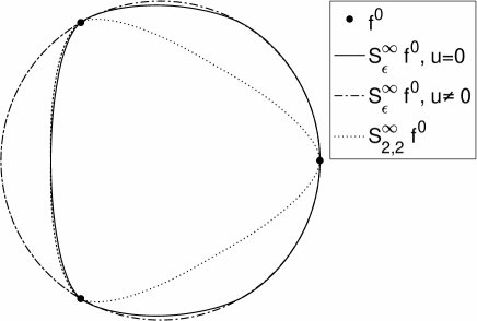
Figure 1. Curves generated by $S_{\epsilon}$ ($\epsilon=1$) and $T_{2,2}$ from an initial sequence $f^{0}=(G_{u}(i))_{i\in\mathds{Z}}$, where $G_{u}(t)=(\cos(\gamma t+u),\sin(\gamma t+u))$, for $u=0$ and $u=u=10^{-5}$. Observe that $S^{\infty}_{\epsilon}f^{0}$ strongly depends on the value of $u$.

This example shows also that $S_{\epsilon}$ is convergent (at least for $\epsilon=1$), a fact that will be proven in the next section, but it is not stable. Nevertheless, in section 8.2 we show that stability holds if the initial data is appropriately restricted.

5. Convergence

In this section we check that the schemes in (29) are of the form (10). Then we prove convergence by checking the conditions in Theorem 3. Observe that

$$\frac{f_{2}-f_{-1}}{f_{1}-f_{0}}=\frac{\nabla f_{1}+\nabla f_{0}+\nabla f_{-1}}{\nabla f_{0}}\quad\longrightarrow\quad\Gamma_{\epsilon}(f_{-1},f_{0},f_{1},f_{2})=\Gamma_{\epsilon}^{[1]}(\nabla f_{-1},\nabla f_{0},\nabla f_{1})$$

with

$$\Gamma^{[1]}_{\epsilon}(f_{-1},f_{0},f_{1})=\begin{cases}\frac{1}{2}\frac{1}{\left(1+\sqrt{1+\frac{f_{-1}+f_{0}+f_{1}}{f_{0}}}\right)^{2}-1},&f_{0}\neq 0\text{ and }1+\frac{f_{-1}+f_{0}+f_{1}}{f_{0}}\geq\epsilon^{2}\\ 0,&f_{-1}\cdot f_{1}\geq 0=f_{0}\\ \frac{1}{16},&\text{ otherwise.}\end{cases}$$

Hence, we can write

(32) $$(S_{\epsilon}f)_{2i+1} =\frac{1}{2}f_{i}+\frac{1}{2}f_{i+1}-\Gamma_{\epsilon}^{[1]}(\nabla f_{i-1},\nabla f_{i},\nabla f_{i+1})\left(\nabla f_{i+1}-\nabla f_{i-1}\right),$$

that is, $S_{\epsilon}$ is of the form (10) with $T=T_{1,1}$ and $\mathcal{F}_{\epsilon}:l_{\infty}(\mathds{Z})\rightarrow l_{\infty}(\mathds{Z})$ given by

(33) $$\mathcal{F}_{\epsilon}(f)_{2i}=0,\qquad\mathcal{F}_{\epsilon}(f)_{2i+1}=\Gamma_{\epsilon}^{[1]}(f_{i-1},f_{i},f_{i+1})\left(f_{i-1}-f_{i+1}\right).$$

Theorem 13.

The scheme $S_{\epsilon}$ is convergent for $\epsilon\in(\sqrt{3}-1,2]$.

Proof.

By (11), $S_{\epsilon}^{[1]}=T_{1,1}^{[1]}+\nabla\mathcal{F}_{\epsilon}$, i.e.

$$(S_{\epsilon}^{[1]}f)_{2i+j}=\frac{1}{2}f_{i}+(-1)^{j}\Gamma^{[1]}_{\epsilon}(f_{i-1},f_{i},f_{i+1})(f_{i-1}-f_{i+1}),\qquad j=0,1.$$

We check conditions C1. and C2. in Theorem 3. For this, we distinguish the following cases:

1. $f_{i}\neq 0$ and $1+(f_{i-1}+f_{i}+f_{i+1})/f_{i}\geq\epsilon^{2}$. In this case we have that

   $$0\leq\Gamma_{\epsilon}^{[1]}(f_{i-1},f_{i},f_{i+1})\leq M_{\epsilon}=\frac{1}{2\epsilon(2+\epsilon)},$$

   hence,

   $$|\mathcal{F}(f)_{2i+1}|\leq 2M_{\epsilon}||f||_{\infty},\qquad|(S_{\epsilon}^{[1]}f)_{2i+j}|\leq||f||_{\infty}(\frac{1}{2}+2M_{\epsilon}).$$

2. $f_{i}=0$, $f_{i+1}\cdot f_{i-1}\geq 0$. Then

   $$\mathcal{F}(f)_{2i+1}=0,\qquad(S^{[1]}f)_{2i+j}=\frac{1}{2}f_{i}\quad\rightarrow\quad|(S^{[1]}f)_{2i+j}|\leq\frac{1}{2}||f||_{\infty},$$

3. otherwise

   $$|\mathcal{F}(f)_{2i+1}|\leq\frac{1}{8}||f||_{\infty},\qquad(S^{[1]}f)_{2i+j}=\frac{1}{2}f_{i}-\frac{1}{16}(f_{i-1}-f_{i+1})\quad\rightarrow\quad|(S^{[1]}f)_{2i+j}|\leq\frac{5}{8}||f||_{\infty}.$$

Then, condition C1. clearly holds for any value of $\epsilon$. In addition, since $0<\epsilon\leq 2$, condition C2. is satisfied with $L=1$ for those values of $\epsilon$ satisfying

$$\max\{\frac{5}{8},\frac{1}{2}+2M_{\epsilon}\}=\frac{1}{2}+2M_{\epsilon}<1\quad\rightarrow\quad\epsilon>\sqrt{3}-1\approx 0.7321.$$

∎

Taking into account Corollary 5, $S_{\epsilon}$ is at least $\mathcal{C}^{\beta-}$, $\beta=-\log_{2}(\frac{1}{2}+\frac{1}{\epsilon(2+\epsilon)})$. This is a conservative result, since $\beta\in(0,0.5)$ for $\epsilon\in(\sqrt{3}-1,2]$. The question of smoothness will be considered in more detail in sections 7 and 9.

On the other hand, we observe that for $\epsilon=\sqrt{3}-1$, the restriction in Proposition 12 is $\cos(|\gamma|)\geq 1-\sqrt{3}$, which is satisfied when $\gamma\in\imath[-\frac{3}{4}\pi,\frac{3}{4}\pi]$, as stated in the introduction.

6. Monotonicity preservation

In applications dealing with increasing (or decreasing) sequences of data, it is often convenient to maintain this feature after recursive refinement. In this section we examine the conditions that guarantee that the family of nonlinear schemes in (10) have this property.

Definition 14.

$S$ is monotonicity preserving if

$$\nabla f^{k}_{i}\geq 0,\,(\leq 0)\quad\forall i\in\mathds{Z}\quad\longrightarrow\quad\nabla f^{k+1}_{i}\geq 0,\,(\leq 0)\quad\forall i\in\mathds{Z}.$$

It is strictly monotonicity preserving if the above relations hold with strict inequalities.

Theorem 15.

$S_{\epsilon}$ is (strictly) monotonicity preserving for $\epsilon\in[0\sqrt{2}]$.

Proof.

Since $\nabla f^{k+1}=\nabla S_{\epsilon}f^{k}=S_{\epsilon}^{[1]}\nabla f^{k}$, and $S^{[1]}(\alpha f)=\alpha S^{[1]}(f)$ $\forall\alpha\in\mathds{R}$, proving that $S_{\epsilon}$ is monotonicity preserving is equivalent to proving that $S^{[1]}_{\epsilon}$ is positivity preserving, i.e.

$$f_{i}\geq 0,\,\forall i\in\mathds{Z}\quad\longrightarrow\quad S_{\epsilon}^{[1]}f_{i}\geq 0,\,\forall i\in\mathds{Z},\qquad\forall f\in l_{\infty}(\mathds{Z}).$$

First, we notice that if $f_{i}\geq 0$ $\forall i\in\mathds{Z}$ and $\epsilon\leq\sqrt{2}$

(34) $$\Gamma^{[1]}_{\epsilon}(f_{i-1},f_{i},f_{i+1}) =\begin{cases}\frac{1}{2}\frac{1}{\left(1+\sqrt{1+\frac{f_{i-1}+f_{i}+f_{i+1}}{f_{i}}}\right)^{2}-1}\,,&f_{i}\neq 0\\ 0\,,&f_{i}=0.\end{cases}$$

Thus, if $f_{i}=0$, $(S_{\epsilon}^{[1]}f)_{2i+j}=0$, $j=0,1$, while for $f_{i}>0$ we can write

$$\Gamma^{[1]}_{\epsilon}(f_{i-1},f_{i},f_{i+1})(f_{i-1}-f_{i+1})=\frac{f_{i}}{2}\frac{f_{i-1}/f_{i}-f_{i+1}/f_{i}}{(\sqrt{2+f_{i-1}/f_{i}+f_{i+1}/f_{i}}+1)^{2}-1}=\frac{f_{i}}{2}H(f_{i-1}/f_{i},f_{i+1}/f_{i})$$

so that

(35) $$(S_{\epsilon}^{[1]}f)_{2i+j}=\frac{1}{2}f_{i}\left(1+(-1)^{j}H(f_{i-1}/f_{i},f_{i+1}/f_{i})\right),\qquad j=0,1,$$

with

(36) $$H(x,y):=\frac{x-y}{(\sqrt{2+x+y}+1)^{2}-1}=\frac{x-y}{2+x+y+2\sqrt{2+x+y}}.$$

By straightforward algebra, we have

$$-1<\frac{-x-y}{2+x+y+2\sqrt{2+x+y}}\leq H(x,y)\leq\frac{x+y}{2+x+y+2\sqrt{2+x+y}}<1,$$

so that $H(x,y)\in(-1,1)$, $\forall x,y\geq 0$. This concludes the proof.

∎

Remark 16.

For strictly positive (negative) data and $\epsilon\in[0,\sqrt{2}]$, $\Gamma_{\epsilon}^{[1]}(f_{i-1},f_{i},f_{i+1})$ is given by (34) (notice that it is independent of the value of $\epsilon$). It can be easily seen that, in this case,

$$|\Gamma_{\epsilon}^{[1]}(f_{i-1},f_{i},f_{i+1})|\leq\frac{1}{2+2\sqrt{2}}$$

hence

$$|(S_{\epsilon}^{[1]}f)_{2i+j}| \leq(\frac{1}{2}+|2\Gamma_{\epsilon}^{[1]}(f_{i-1},f_{i},f_{i+1})|)\|f\|_{\infty}\leq(\frac{1}{2}+\frac{1}{1+\sqrt{2}})\|f\|_{\infty}.$$

Condition C2. in Theorem 3 is, thus, fulfilled with $L=1$ and $\eta=\frac{1}{2}+\frac{1}{1+\sqrt{2}}<1$. Hence, if $f^{0}$ is a strictly monotone sequence, and $\epsilon\in[0,\sqrt{2}]$, $S_{\epsilon}^{\infty}f^{0}$ is a continuous function that preserves the monotonicity properties of the initial data. This function does not depend on the value chosen for the parameter $\epsilon$.

7. Smoothness

In this section we examine the smoothness of the schemes $S_{\epsilon}$. We shall see first that $S_{\epsilon}$ admits a first divided difference scheme, which relates the divided differences of the data produced by $S_{\epsilon}$ at consecutive resolution levels.

Divided differences at level $k$ are defined as $d^{k}_{i}:=2^{k}\nabla f^{k}_{i},\,{i\in\mathds{Z}}$, where $f^{k}=S_{\epsilon}f^{k-1}$, $k\geq 1$. Since $S^{[1]}_{\epsilon}$ satisfies $2S^{[1]}_{\epsilon}f=S^{[1]}_{\epsilon}2f$, $\forall f\in l_{\infty}(\mathds{Z})$, we can write

$$2^{k+1}\nabla f^{k+1}=2S^{[1]}_{\epsilon}2^{k}\nabla f^{k}\quad\Longrightarrow d^{k+1}=2S^{[1]}_{\epsilon}d^{k}$$

so that the first divided difference scheme can be defined as $S_{\epsilon}^{(1)}:=2S_{\epsilon}^{[1]}$. It is well known (see e.g. [12]) that if $S_{\epsilon}^{(1)}$ is a convergent subdivision scheme, then $S_{\epsilon}$ converges to $\mathcal{C}^{1}$ functions and

$$((S_{\epsilon}^{(1)})^{\infty}d^{0})(t)=\frac{d}{dt}(S^{\infty}_{\epsilon}f^{0})(t).$$

In this section we study the conditions that guarantee convergence of the subdivision scheme $S_{\epsilon}^{(1)}$. As in [12, 17], for a given $d^{0}$ we shall define $\mathbb{P}^{k}(t)$ as the continuous piecewise linear function such that

(37) $$\mathbb{P}^{k}(i2^{-k})=d^{k}_{i},\qquad\forall{i\in\mathds{Z}}$$

$d^{k}=S^{(1)}_{\epsilon}d^{k-1}$, $k\geq 1$, and study the conditions that ensure that $(\mathbb{P}^{k})_{k\geq 0}$ is a Cauchy sequence.

Observe that

$$\left\|\mathbb{P}^{k+1}-\mathbb{P}^{k}\right\|_{\infty}=\sup_{i\in\mathds{Z}}\max\{|d^{k+1}_{2i}-d^{k}_{i}|,|d^{k+1}_{2i+1}-\frac{1}{2}(d^{k}_{i}+d^{k}_{i+1})|\}$$

and that, using that $d^{k}_{i}=\frac{1}{2}(d^{k+1}_{2i}+d^{k+1}_{2i+1})$,

$$|d^{k+1}_{2i}-d^{k}_{i}| =\frac{1}{2}|d^{k+1}_{2i+1}-d^{k}_{2i}|\leq\frac{1}{2}\left\|\nabla d^{k+1}\right\|_{\infty}$$

$$|d^{k+1}_{2i+1}-\frac{1}{2}(d^{k}_{i}+d^{k}_{i+1})| =|d^{k+1}_{2i+1}-\frac{1}{4}(d^{k+1}_{2i}+d^{k+1}_{2i+1}+d^{k+1}_{2i+2}+d^{k+1}_{2i+3})|$$

$$=\frac{1}{4}|d^{k+1}_{2i+1}-d^{k+1}_{2i}+2(d^{k+1}_{2i+1}-d^{k+1}_{2i+2})+d^{k+1}_{2i+2}-d^{k+1}_{2i+3}|\leq\left\|\nabla d^{k+1}\right\|_{\infty}.$$

As a consequence, we have that $\left\|\mathbb{P}^{k+1}-\mathbb{P}^{k}\right\|_{\infty}\leq\left\|\nabla d^{k+1}\right\|_{\infty}$, so that the convergence of $S_{\epsilon}^{(1)}$ follows from proving that $\left\|\nabla d^{k}\right\|_{\infty}\overset{k\to\infty}{\longrightarrow}0$. Notice that for $d^{k}_{i}\neq 0$

$$d^{k}_{i+1}-d^{k}_{i}=d^{k}_{i}\left(\frac{d^{k}_{i+1}}{d^{k}_{i}}-1\right)$$

hence, we might prove the desired result by checking the following two conditions

(38) $$\text{(a) }\quad\left\|d^{k}\right\|_{\infty}<M<\infty,\quad\forall k\geq 0\qquad\text{(b) }\quad\lim_{k\to\infty}\sup_{i\in\mathds{Z}}|\frac{d^{k}_{i+1}}{d^{k}_{i}}-1|=0,$$

at least for a restricted class of initial data $d^{0}$ such that $d^{0}_{i}\neq 0$, $\forall{i\in\mathds{Z}}$.

Notice that if the initial data satisfy $d^{0}_{i}>0(<0)$, $\forall{i\in\mathds{Z}}$ and $\epsilon\in[0,\sqrt{2}]$, then Theorem 15 ensures that $d^{k}_{i}\neq 0$ $\forall i,k$. Since the repeated application of $S_{\epsilon}$ preserves strict monotonicity, we have that $d^{k}_{i}>0(<0)$, $\forall k\geq 0\,\forall{i\in\mathds{Z}}$.

Hence, throughout this section we shall assume that we have strictly monotone data and we shall silently assume that $\epsilon\in[0,\sqrt{2}]$. In Remark 16 we observed that, in this case, $S_{\epsilon}$ does not depend on the value of $\epsilon$ and is convergent. From (35) we get the expression of $S_{\epsilon}^{(1)}$ in this case,

(39) $$(S_{\epsilon}^{(1)}d)_{2i+j}=\Psi_{j}(d_{i-1},d_{i},d_{i+1}):=d_{i}\left(1+(-1)^{j}H(\frac{d_{i}}{d_{i-1}},\frac{d_{i+1}}{d_{i}})\right),\qquad j=0,1,$$

where $H(x,y)$ is defined in (36). Notice that $\Psi_{j}$, $j=0,1$, are 1-homogeneous functions. In addition, the results obtained in the previous section ensure that $\Psi_{j}:\mathds{R}^{3}_{+}\rightarrow\mathds{R}_{+}$, $j=0,1$, ($R_{+}=(0,+\infty)$), i.e. they are positive functions, when restricted to positive data. They are also smooth, being compositions of smooth functions that are always well-defined for positive data.

We shall examine next what are the conditions to ensure that (38)-(b) is satisfied. As in [17], given an initial sequence $d^{0}$, with $d^{0}_{i}>0(<0)$, and $d^{k}=S_{\epsilon}^{(1)}d^{k-1}$, $k\geq 1$, we define

(40) $$R^{k}_{i}:=\frac{d^{k}_{i+1}}{d^{k}_{i}},\quad r^{k}_{i}=1/R^{k}_{i},\qquad\rho^{k}:=\sup_{i\in\mathds{Z}}\left\{\left|r^{k}_{i}-1\right|,\left|R^{k}_{i}-1\right|\right\},$$

and study the behavior of the sequence $\rho^{k}$. Obviously, proving that $\lim_{k\rightarrow\infty}\rho^{k}=0$ leads to (38)-(b). As a previous step, we need to restrict the class of initial data to ensure that $\rho^{k}<+\infty,\quad\forall k\geq 0$.

Lemma 17.

Let $d^{k}\in l_{\infty}(\mathds{Z})$, $d^{k}_{i}>0(<0)$, and $d^{k+1}=S_{\epsilon}^{(1)}d^{k}$, $k\geq 0$. Then, with the definitions in (39)-(40), if $\rho^{k}<+\infty$, then $\rho^{k+1}<+\infty$

Proof.

Using (39) and (40) we can write

$$R^{k+1}_{2i}=\frac{\Psi_{1}(d^{k}_{i-1},d^{k}_{i},d^{k}_{i+1})}{\Psi_{0}(d^{k}_{i-1},d^{k}_{i},d^{k}_{i+1})}=\frac{d^{k}_{i}\Psi_{1}(d^{k}_{i-1}/d^{k}_{i},1,d^{k}_{i+1}/d^{k}_{i})}{d^{k}_{i}\Psi_{0}(d^{k}_{i-1}/d^{k}_{i},1,d^{k}_{i+1}/d^{k}_{i})}=\frac{\Psi_{1}(r^{k}_{i-1},1,R^{k}_{i})}{\Psi_{0}(r^{k}_{i-1},1,R^{k}_{i})}=:G_{1}(r^{k}_{i-1},R^{k}_{i}).$$

Since $G_{1}$ is smooth when applied to positive data, applying the Mean Value Theorem we get

(41) $$R^{k+1}_{2i}-1 =G_{1}(r^{k}_{i-1},R^{k}_{i})-G_{1}(1,1)=\nabla G_{1}(\hat{r}^{k}_{i},\hat{R}^{k}_{i})\cdot\left((r^{k}_{i-1},R^{k}_{i})-(1,1)\right)$$

where $(\hat{r}^{k}_{i},\hat{R}^{k}_{i})$ belongs to the segment joining the points $(1,1)$ and $(r^{k}_{i-1},R^{k}_{i})$. Hence,

(42) $$|R^{k+1}_{2i}-1| \leq\rho^{k}\max_{r,R\in K}\|\nabla G_{1}(r,R)\|_{1},$$

where $K$ is the ball of center $(1,1)$ and radius $\rho^{k}$. The same type of argument can be used to obtain similar bounds for $|R^{k+1}_{2i+1}-1|$ and $|r^{k+1}_{2i+j}-1|$, $j=0,1$, which proves the result. ∎

Remark 18.

Given $d\in l_{\infty}(\mathds{Z})$ with $d_{i}>0(<0)$ $\forall i\in\mathds{Z}$, we define

$$\rho(d):=\sup_{i\in\mathds{Z}}\left\{\left|r_{i}-1\right|,\left|R_{i}-1\right|\right\},\qquad R_{i}:=\frac{d_{i+1}}{d_{i}},\quad r_{i}=1/R_{i}.$$

Then, according to the previous lemma, $\rho:l_{\infty}^{+}(\mathds{Z})\rightarrow\mathds{R}_{+}$, where

$$l_{\infty}^{+}(\mathds{Z})=\{d\in l_{\infty}(\mathds{Z}):\,d_{i}\cdot d_{i+1}>0\,\forall i\in\mathds{Z}\text{ and }\sup_{i\in\mathds{Z}}\left\{\left|\frac{d_{i}}{d_{i+1}}-1\right|,\left|\frac{d_{i+1}}{d_{i}}-1\right|\right\}<+\infty\}$$

and if $\rho^{0}=\rho(d^{0})$ then $\rho^{k}$ in (40) satisfies $\rho^{k}=\rho(d^{k})$ with $d^{k}=S_{\epsilon}^{(1)}d^{k-1}$, $k\geq 1$.

We will show that, at least under an appropriate restriction on $\rho^{0}=\rho(d^{0})$, the sequence $(\rho^{k})_{k\geq 0}$ converges to zero. As a first attempt, we try to find $\eta$ and $\delta$ such that

(43) $$\rho^{0}<\delta\quad\Longrightarrow\quad\rho^{k+1}\leq\eta\rho^{k},\qquad\forall k\geq 0.$$

Obviously, if we could prove (43) with $0<\eta<1$, we would obtain the desired result. However, we shall see that we can only expect (43) to hold for values of $\eta$ greater than 1. Nevertheless, we will be able to prove that given $\eta\in(\frac{3}{4},1)$ there exists $\delta_{\eta}$ such that

(44) $$\rho^{0}<\delta_{\eta}\quad\Longrightarrow\quad\rho^{k+2}\leq\eta\rho^{k},\qquad\forall k\geq 0,$$

which will allow us to prove the required convergence result.

Let us start by analyzing (43). From (41), and taking into account that $||\nabla G_{1}(1,1)||_{1}=\frac{1}{2}$ (see the Appendix for details), given $\eta\in(\frac{1}{2},1)$ we can find $\delta_{1}>0$ such that

$$\|(r,R)-(1,1)\|_{\infty}<\delta_{1}\quad\Longrightarrow\quad\|\nabla G_{1}(r,R)\|_{1}\leq\eta.$$

Hence, from (42), we get that if $\rho^{k}<\delta_{1}$

$$|R^{k+1}_{2i}-1| \leq\rho^{k}\max_{r,R\in K}\|\nabla G_{1}(r,R)\|_{1}\leq\eta\,\rho^{k}.$$

On the other hand, the same type of arguments for $R^{k+1}_{2i+1}$ lead to the following:

$$R^{k+1}_{2i+1}=\frac{\Psi_{0}(d^{k}_{i},d^{k}_{i+1},d^{k}_{i+2})}{\Psi_{1}(d^{k}_{i-1},d^{k}_{i},d^{k}_{i+1})}=\frac{\Psi_{0}\left(1,\frac{d_{i+1}^{k}}{d_{i}^{k}},\frac{d_{i+2}^{k}}{d_{i+1}^{k}}\frac{d_{i+1}^{k}}{d_{i}^{k}}\right)}{\Psi_{1}\left(\frac{d_{i-1}^{k}}{d_{i}^{k}},1,\frac{d_{i+1}^{k}}{d_{i}^{k}}\right)}=:G_{2}(r^{k}_{i-1},R^{k}_{i},R^{k}_{i+1}).$$

It is shown in the appendix that $\|\nabla G_{2}(1,1,1)\|_{1}=1$, thus $|R^{k+1}_{2i+1}-1|$ cannot be bounded as before using any $\eta<1$ and we cannot expect (43) to hold for any $\eta<1$. We then turn to analyze (44).

Lemma 19.

Given $\eta\in(\frac{3}{4},1)$, there exists $\delta_{\eta}>0$ such that if $\rho^{0}<\delta_{\eta}$ then $\rho^{k+2}\leq\eta\rho^{k},\qquad\forall k\geq 0.$

Proof.

We shall use the same technique as before to examine

$$|R^{k+2}_{4i+j}-1|\quad\text{and}\quad|r^{k+2}_{4i+j}-1|\qquad j=0,1,2,3.$$

Let us denote the four rules that define $(S_{\epsilon}^{[1]})^{2}$ as follows:

$$(S_{\epsilon}^{[1]}S_{\epsilon}^{[1]}d)_{4i+j}=:\Psi^{2}_{j}(d_{i-2},d_{i-1},d_{i},d_{i+1},d_{i+2}),\qquad j=0,1,2,3$$

where, without loss of generality, we have assumed that $\Psi^{2}_{j}:\mathds{R}^{5}_{+}\rightarrow\mathds{R}_{+}$, $j=0,1,2,3$. The specific form of these (smooth) functions can be found in the Appendix, as well as the required computations, which are lengthy but straightforward. In what follows we give only a sketch of the proof.

Since the functions $\Psi_{j}^{2}$ are 1-homogeneous and smooth, we can write

$$\begin{cases}R^{k+2}_{4i+j}&=\displaystyle{\frac{\Psi^{2}_{j+1}(d_{i-2}^{k},\cdots,d^{k}_{i+2})}{\Psi^{2}_{j}(d_{i-2}^{k},\cdots,d^{k}_{i+2})}}=G^{2}_{j}(r^{k}_{i-2},r^{k}_{i-1},R^{k}_{i},R^{k}_{i+1}),\\[10.0pt] r^{k+2}_{4i+j}&=\displaystyle{\frac{1}{R^{k+2}_{4i+j}}=\frac{1}{G^{2}_{j}(r^{k}_{i-2},r^{k}_{i-1},R^{k}_{i},R^{k}_{i+1})}},\end{cases}\quad j=0,1,2,3.$$

It is easy to see that $G^{2}_{j}(\mathds{1}_{4})=1$, $\mathds{1}_{4}:=(1,1,1,1)$. In addition,

$$\nabla\frac{1}{G^{2}_{j}}(\mathds{1}_{4})=-\frac{\nabla G_{j}^{2}(\mathds{1}_{4})}{G_{j}^{2}(\mathds{1}_{4})^{2}}=-\nabla G_{j}^{2}(\mathds{1}_{4}).$$

In the appendix we carry out all the necessary computations to obtain the values of $\|\nabla G^{2}_{j}(\mathds{1}_{4})\|_{1}$, which are displayed in Table 1.

$j$	0	1	2	3
$\|\nabla G^{2}_{j}(\mathds{1}_{4})\|_{1}$	5/16	1/4	5/16	3/4

Table 1. The 1-norm of the ratio functions $G^{2}_{j}$ for $j=0,1,2,3$.

The functions $G^{2}_{j}:\mathds{R}^{4}_{+}\rightarrow\mathds{R}_{+}$ are smooth and satisfy $G^{2}_{j}(\mathds{1}_{4})=1$, $\|\nabla G^{2}_{j}(\mathds{1}_{4})\|_{1}\leq\|\nabla G^{2}_{3}(\mathds{1}_{4})\|_{1}=\frac{3}{4}$. Then using the Mean Value Theorem as before we know that, given $\eta\in(\frac{3}{4},1)$ exists $\delta$ such that if $\rho^{k}<\delta$

$$\rho^{k+2}=\max_{{i\in\mathds{Z}}}\max_{0\leq j\leq 3}\{|R^{k+2}_{4i+j}-1|,|r^{k+2}_{4i+j}-1|\}\leq\eta\rho^{k}.$$

To conclude the proof, we notice that given $\eta\in(3/4,1)$ and $k$ such that $\rho^{k}<\delta$, we have that $\rho^{k+2}<\eta\rho^{k}<\delta$. Thus, if $\rho^{0},\rho^{1}<\delta$, then $\rho^{k}<\delta$ for all $k\geq 0$. Since we know that we can find $\delta^{1}>0$ and $\eta^{1}>1$ such that if $\rho^{0}<\delta^{1}$, then $\rho^{1}\leq\eta^{1}\rho^{0}$, taking $\delta_{\eta}:=\min\{\delta/\eta^{1},\delta^{1}\}$ we have that if $\rho^{0}<\delta_{\eta}\leq\delta^{1}$, then $\rho^{1}<\eta^{1}\rho^{0}<\eta^{1}\delta_{\eta}\leq\eta^{1}\delta/\eta^{1}=\delta$. Therefore if $\rho^{0}<\delta_{\eta}$, then $\rho^{0},\rho^{1}<\delta$ and the result holds. ∎

Then, we can prove that $\rho^{k}$ decreases at least as fast as $\eta^{\frac{k}{2}}$.

Proposition 20.

Given $\eta\in(\frac{3}{4},1)$, there exists $\delta_{\eta}>0$ such that if $\rho^{0}<\delta_{\eta}$,

$$\rho^{k+1}<\eta^{\frac{k}{2}}\max\{\rho^{1},\rho^{0}\},\qquad\forall k\geq 0.$$

Proof.

Given $\eta\in(\frac{3}{4},1)$, we apply the previous Lemma and consider separately the cases of $k$ even or odd. Then, for $\rho^{0}<\delta_{\eta}$,

$$k=2k^{\prime}\quad\longrightarrow\quad\rho^{k+1} =\rho^{2k^{\prime}+1}\leq\eta\rho^{2(k^{\prime}-1)+1}\leq\cdots\leq\eta^{k^{\prime}}\rho^{1}=\eta^{\frac{k}{2}}\rho^{1},$$

$$k=2k^{\prime}+1\quad\longrightarrow\quad\rho^{k+1} =\rho^{2(k^{\prime}+1)}\leq\eta\rho^{2k^{\prime}}\leq\cdots\leq\eta^{k^{\prime}+1}\rho^{0}<\eta^{\frac{k^{\prime}+1}{2}}\rho^{0}<\eta^{k/2}\rho^{0}.$$

∎

The next result shows that the growth of the divided finite differences at each level or refinement also depends on $\rho^{k}$. Then we can prove (38)-(a).

Lemma 21.

Assume that $d^{k}_{i}>0$ (or $d^{k}_{i}<0$), $\forall{i\in\mathds{Z}}$. Then,

$$(1-\frac{\rho^{k}}{1+\sqrt{2}})|d^{k}_{i}|\leq|d^{k+1}_{2i+j}|\leq(1+\frac{\rho^{k}}{1+\sqrt{2}})|d^{k}_{i}|,\qquad j=0,1.$$

Proof.

As stated in (39), for this type of data

$$d^{k+1}_{2i+j}=d^{k}_{i}\left(1+(-1)^{j}H(r^{k}_{i-1},R^{k}_{i})\right),\qquad j=0,1.$$

It is very easy to check that $\forall x,y\geq 0$

$$|H(x,y)|\leq\frac{1}{2+2\sqrt{2}}|x-y|\leq\frac{1}{1+\sqrt{2}}\max\{|x-1|,|y-1|\}.$$

Thus $|H(r^{k}_{i-1},R^{k}_{i})|\leq\frac{\rho^{k}}{1+\sqrt{2}}$ $\forall{i\in\mathds{Z}}$, and

$$1-\frac{\rho^{k}}{1+\sqrt{2}}\leq 1-|H(r^{k}_{i-1},R^{k}_{i})|\leq\frac{|d^{k+1}_{2i+j}|}{|d^{k}_{i}|}\leq 1+|H(r^{k}_{i-1},R^{k}_{i})|\leq 1+\frac{\rho^{k}}{1+\sqrt{2}}.$$

∎

Proposition 22.

Let $d^{0}$ be a strictly positive (negative) sequence and $d^{k}=S^{(1)}_{\epsilon}d^{k-1}$, $k\geq 1$. Given $\eta\in(\frac{3}{4},1)$, $\exists\delta_{\eta}>0$ such that if $\rho^{0}<\delta_{\eta}$ then the sequence $(d^{k})_{k=0}^{\infty}$ is uniformly bounded.

Proof.

By Lemma 21

$$\left\|d^{k+1}\right\|_{\infty}\leq(1+\frac{\rho^{k}}{1+\sqrt{2}})\left\|d^{k}\right\|_{\infty},\quad\rightarrow\quad\left\|d^{k}\right\|_{\infty}\leq\left\|d^{0}\right\|_{\infty}\prod_{l=0}^{k-1}(1+\frac{\rho^{l}}{1+\sqrt{2}}).$$

Applying Proposition 20, there exists $\delta_{\eta}>0$ such that if $\rho^{0}<\delta_{\eta}$,

$$\left\|d^{k}\right\|_{\infty}\leq\left\|d^{0}\right\|_{\infty}\prod_{l=0}^{k-1}(1+c\eta^{l/2}),\qquad c=\max\{\rho^{1},\rho^{0}\}\frac{\eta^{-1/2}}{1+\sqrt{2}}.$$

Observe that

$$\prod_{l=0}^{k-1}(1+c\eta^{l/2})=\exp(\log(\prod_{l=0}^{k-1}(1+c\eta^{l/2})))=\exp(\sum_{l=0}^{k-1}\log(1+c\eta^{l/2}))\leq\exp(\sum_{l=0}^{k-1}c\eta^{l/2}),$$

since $\log(1+t)\leq t$, $\forall t\geq 0$. Then $\left\|d^{k}\right\|_{\infty}\leq\left\|d^{0}\right\|_{\infty}\exp(\frac{c}{1-\sqrt{\eta}}),$ which proves the result. ∎

Theorem 23.

Let $d^{0}$ be a strictly positive (negative) sequence and $d^{k}=S^{(1)}_{\epsilon}d^{k-1}$, $k\geq 1$. There exists $\bar{\delta}>0$ such that if $\rho^{0}<\bar{\delta}$, then $S_{\epsilon}^{(1)}d^{0}$ converges to a $\mathcal{C}^{\alpha-}$ function, with $\alpha=1-\frac{1}{2}log_{2}3$.

Proof.

As we observed previously, the piecewise linear functions $\mathbb{P}^{k}(t)$ in (37) satisfy that

$$\left\|\mathbb{P}^{k+1}-\mathbb{P}^{k}\right\|_{\infty}\leq\left\|\nabla d^{k+1}\right\|_{\infty}.$$

Since $|\nabla d^{k}_{j}|=|d^{k}_{j+1}-d^{k}_{j}|=|d^{k}_{j}|\left|\frac{d^{k}_{j+1}}{d^{k}_{j}}-1\right|,$ by Lemma 22 and Proposition 20, given $\eta\in(\frac{3}{4},1)$, $\exists\delta_{\eta}>0$ and $C>0$ such that if $\rho^{0}<\delta_{\eta}$ then

$$\left\|\mathbb{P}^{k+1}-\mathbb{P}^{k}\right\|_{\infty}\leq\left\|\nabla d^{k+1}\right\|_{\infty}\leq\left\|d^{k+1}\right\|_{\infty}\rho^{k+1}\leq C\eta^{\frac{k}{2}}.$$

Then, by slightly modifying the proof of Corollary 3.3 in [12] we get that $S^{(1)}_{\epsilon}d^{0}$ is $\mathcal{C}^{-\log_{2}(\sqrt{\eta})}$ smooth.

Let us define $\bar{\delta}:=\sup_{\frac{3}{4}<\eta<1}\delta_{\eta}$. If $\rho^{0}<\bar{\delta}$, then $\rho^{0}<\delta_{\eta_{0}}$ for some $\eta_{0}\in(\frac{3}{4},1)$ and, by the properties of $\delta_{\eta_{0}}$, we also have that $\rho^{k}\leq C\eta_{0}^{k/2}$ and, as a consequence, $S^{(1)}d^{0}$ is $\mathcal{C}^{-\log_{2}(\sqrt{\eta_{0}})}$ smooth. Let us consider now any other $\eta\in(\frac{3}{4},1)$, and its ’associated’ $\delta_{\eta}$. Let $k_{0}$ be s.t. $\eta_{0}^{k/2}<\delta_{\eta}/C$, $\forall k\geq k_{0}$. Then $\rho^{k}<\delta_{\eta}$, $\forall k\geq k_{0}$ and, by the same arguments used throughout this section, $\rho^{k}\leq C^{\prime}\eta^{\frac{k}{2}}$, $\forall k\geq k_{0}$, $C^{\prime}>0$. But this decay rate on the $\rho^{k}$ (for $k$ large enough) also implies that the smoothness of the limit function is $\mathcal{C}^{-\log_{2}(\sqrt{\eta})}$. Since $\eta$ is arbitrary in $(\frac{3}{4},1)$, we conclude that the limit functions are at least $\mathcal{C}^{\alpha-}$, with $\alpha=-\frac{1}{2}\log_{2}(\frac{3}{4})=1-\frac{1}{2}\log_{2}(3)\cong 0.2$. ∎

According to the previous theorem, the smoothness of $S_{\epsilon}$ for strictly monotone data is at least $C^{1+\alpha-}$, as long as the initial data satisfies the ’technical’ additional condition $\rho(d^{0})<\bar{\delta}$. Notice that

$$\rho(d)<\bar{\delta}\quad\equiv\quad\max_{i}\{\frac{|d_{i+1}-d_{i}|}{|d_{i}|},\frac{|d_{i+1}-d_{i}|}{|d_{i+1}|}\}<\bar{\delta},$$

hence, it is quite straightforward to see that the required technical condition may, in fact, be easily achieved for smooth (strictly increasing) data. Indeed, if $f=F|_{2^{-k}\mathds{Z}}$, then $d_{i}=2^{k}\nabla f_{i}=F^{\prime}(ih)+O(h)$, with $h=2^{-k}$, and

$$\frac{|d_{i+1}-d_{i}|}{|d_{i}|}\approx h\frac{|F^{\prime\prime}(ih+\xi)|+O(h)}{|F^{\prime}(ih)|+O(h)},\quad\xi\in[0,h].$$

Hence, for strictly monotone smooth initial data such that $|F^{\prime}|>\theta>0$, we get that $\rho(d)$ is $O(h)$ and there should be no problem in adjusting $h$ (the initial sampling) in order to fulfill the required condition.

In addition, taking into account the proof of Lemma 19, it is possible to give an estimate of the value of $\bar{\delta}$ with the aid of Wolfram Mathematica by checking what is the largest value of $\delta>0$ satisfying

$$\|\nabla G^{2}_{j}(\bar{x})\|_{1}<1,\quad\|\nabla\frac{1}{G^{2}_{j}}(\bar{x})\|_{1}<1,\quad\forall\,\bar{x}:||\bar{x}-\mathds{1}_{4}||_{\infty}<\delta.$$

According to our computations, we estimate that $\bar{\delta}\approx 0.18$.

8. Stability and Approximation order

Stability and approximation order are also important properties of a subdivision scheme. Both concepts are enclosed below for completeness.

Definition 24.

(Lipschitz) Stability. We say that a convergent subdivision scheme is stable if

$$\left\|S^{\infty}f-S^{\infty}g\right\|_{\infty}\leq C\left\|f-g\right\|_{\infty},\qquad f,g\in l_{\infty}(\mathds{Z}).$$

Definition 25.

Approximation order. A convergent subdivision scheme has approximation order $r$ if for any sufficiently smooth function, $F$, there exists $h_{0}$ such that

$$\left\|F-(S^{\infty}f^{0})(\bullet/h)\right\|_{\infty}\leq Ch^{r},\qquad f^{0}=F|_{h\mathds{Z}},\qquad\forall h\leq h_{0}.$$

The approximation order measures the approximation capabilities of the subdivision process, that is, the ability to ensure that smooth behavior is adequately represented. Since the explicit expression of $S^{\infty}$ is usually unknown, the approximation capabilities of a subdivision scheme are often analyzed by considering instead the approximation order after one step.

Definition 26.

Approximation order after one step. A subdivision scheme has approximation order $r$ after one step if for any sufficiently smooth function, $F$, there exists $h_{0}$ such that

$$\left\|F|_{\frac{h}{2}\mathds{Z}}-Sf\right\|_{\infty}\leq Ch^{r},\qquad f=F|_{h\mathds{Z}},\qquad\forall h\leq h_{0}.$$

It is well known that the approximation order of a subdivision scheme after one step determine the order of approximation of the scheme, provided the scheme is stable (Theorem 2.4.10 of [17]). The order of approximation and the stability of nonlinear schemes are often studied together [2, 3, 9].

For linear stationary subdivision schemes, Lipschitz stability is a consequence of convergence, but this is not the case for nonlinear subdivision [1, 5, 16]. Some theory was developed and successfully applied on several instances [1, 3, 5, 7, 9, 17].

We have already observed that the nonlinear schemes $S_{\epsilon}$ in (29) are not stable for general data (see Figure 1). However, as in section 7, we shall be able to prove stability for a conveniently restricted class of strictly monotone data. For such data, the order of approximation can be obtained by the usual, Taylor-like, one-step approximation results [9].

8.1. Approximation order

Theorem 27.

Let $F$ be a smooth function with $|F^{\prime}|>\theta>0$, and let $f=(F(ih))_{i\in\mathds{Z}}$. Then, for any $\epsilon\in[0,\sqrt{2}]$ we have

$$||F|_{\frac{h}{2}\mathds{Z}}-S_{\epsilon}f||_{\infty}\leq Ch^{4}.$$

Proof.

Clearly $f^{0}=(F(ih))_{i\in\mathds{Z}}$ is a strictly monotone sequence. Since $(S_{\epsilon}f^{0})_{2i}=f^{0}_{i}=F(ih)=F(2ih/2)$, we only need to measure the distance between $(S_{\epsilon}f)_{2i+1}$ and $F(\xi_{i})$, $\xi_{i}=(2i+1)h/2=(i+1/2)h$. By taking a formal Taylor series expansion we find

$$(S_{\epsilon}f)_{2i+1}=F(\xi_{i})+\frac{3h^{4}}{128}\left(\frac{F^{(3)}(\xi_{i})F^{\prime\prime}(\xi_{i})}{F^{\prime}(\xi_{i})}-F^{(4)}(\xi_{i})\right)+O\left(h^{5}\right).$$

∎

8.2. Stability

In [1, 3, 9], stability is proved using a result similar to Theorem 3 (see for instance Theorem 1 of [9]), which requires that the scheme is of the form (10).

Theorem 28.

Let $S$ be of the form (10). $S$ is stable provided that

S1. $$\qquad\exists M>0: ||\mathcal{F}(f)-\mathcal{F}(g)||_{\infty}\leq M||f-g||_{\infty} \forall f,g\in l^{\infty}(\mathbb{Z})$$

S2. $$\qquad\exists L>0,\,\,0<\eta<1: \left\|(S^{[1]})^{L}f-(S^{[1]})^{L}g\right\|_{\infty}\leq\eta\left\|f-g\right\|_{\infty} \forall f,g\in l^{\infty}(\mathbb{Z})$$

Notice that S1 and S2 are Lipschitz-type conditions on $\mathcal{F}$ and $(S^{[1]})^{L}$. We have already observed that $S_{\epsilon}$ is not stable (see Figure 1). The reason behind the lack of stability can be traced back to the fact that $\Gamma_{\epsilon}$ is not a continuous function, so that S1 and S2 cannot be fulfilled, in general.

In section 7 we have seen that if the initial data is a strictly monotone sequence and $\epsilon\in[0,\sqrt{2}]$, the subdivision rules of $S^{(1)}_{\epsilon}$ are smooth, positive, functions. In this case, the two conditions in Theorem 28 could be fulfilled, hence, for the rest of the section we shall (silently) assume that $\epsilon\in[0,\sqrt{2}]$, and restrict our attention to strictly monotone data.

In [3, 9, 16], the authors use the theory of Generalized Jacobians to prove condition S2 for nonlinear schemes defined by piecewise smooth subdivision rules. The main argument used in these references derives from the following inequality

(45) $$\left\|(S^{[1]})^{L}f-(S^{[1]})^{L}g\right\|_{\infty}\leq\left\|f-g\right\|_{\infty}\sup_{t\in[0,1]}\|DS^{[1]}(\tau^{L-1}(t))\cdots DS^{[1]}(\tau^{1}(t))DS^{[1]}(\tau^{0}(t))\|_{\infty},$$

where $DS^{[1]}$ is the (generalized) Jacobian of $S^{[1]}$ (see [16] or the appendix in [9] for details) and

(46) $$\tau^{0}(t)=(1-t)f+tg,\qquad\tau^{k}(t)=S^{[1]}(\tau^{k-1}(t)).$$

In our case, the (smooth) subdivision rules of $S^{[1]}_{\epsilon}=\frac{1}{2}S^{(1)}_{\epsilon}$ are $\frac{1}{2}\Psi_{0},\frac{1}{2}\Psi_{1}$, with $\Psi_{j}$ defined in (39) and $DS_{\epsilon}^{[1]}$ is the bi-infinite matrix with the following non-zero entries (we use Matlab notation, as in [3, 9]))

(47) $$(DS_{\epsilon}^{[1]})_{[2i+j,i-1:i+2]}=\frac{1}{2}\nabla\Psi_{j}(f_{i-1},f_{i},f_{i+1}),\qquad j=0,1.$$

To check (45), we need the following preliminary results.

Lemma 29.

Given $\delta>0$, and $f,g\in l_{\infty}(\mathds{Z})$ such that $f_{i},g_{i}>0(<0)$ $\forall i\in\mathds{Z}$, we have that

(48) $$\rho(f),\rho(g)<\delta\quad\rightarrow\quad\rho((1-t)f+tg)<\delta\quad\forall t\in[0,1],$$

where $\rho$ defined in Remark 18.

Proof.

Notice first that for any $u\in l_{\infty}(\mathds{Z})$

$$\rho(u)<\delta\quad\equiv\quad|u_{i+1}-u_{i}|\leq\delta|u_{j}|,\qquad\forall{i\in\mathds{Z}},\,j=i,i+1.$$

To prove the result, we shall check that $\forall{i\in\mathds{Z}}$ and $t\in[0,1]$,

$$|((1-t)f_{i+1}+tg_{i+1})-((1-t)f_{i}+tg_{i})|<\delta|(1-t)f_{j}+tg_{j}|,\qquad j=i,i+1.$$

The cases $t=0$ and $t=1$ are trivial. For, $t\in(0,1)$, since $(1-t)>0$ we can write

$$|((1-t)f_{i+1}+tg_{i+1})-((1-t)f_{i}+tg_{i})| \leq(1-t)|f_{i+1}-f_{i}|+t|g_{i+1}-g_{i}|$$

$$\leq\delta\left((1-t)|f_{j}|+t|g_{j}|\right)=\delta|(1-t)f_{j}+tg_{j}|,\quad j=i,i+1,$$

where we have used that $|f_{l}+g_{l}|=|f_{l}|+|g_{l}|$ $\forall l\in\mathds{Z}$, since all components have the same sign. ∎

Proposition 30.

Let us consider $\eta\in(\frac{5}{8},1)$ and $\delta\in(0,\bar{\delta})$, where $\bar{\delta}$ is defined in Theorem 23. Then $\exists\,K_{\delta}$ such that $\forall f^{0},g^{0}$ satisfying $f_{i}^{0},g_{i}^{0}>0(<0)$ and $\rho(f^{0}),\rho(g^{0})<\delta$

$$\sup_{t\in[0,1]}\|DS_{\epsilon}^{[1]}(\tau^{k}(t))\|_{\infty}\leq\eta,\qquad\forall k\geq K_{\delta},$$

with $\tau^{k}$ in (46).

Proof.

From (47), we have

(49) $$\|DS_{\epsilon}^{[1]}(\tau^{k}(t))\|_{\infty}=\sup_{i\in\mathds{Z},\,j=0,1}\|\frac{1}{2}\nabla\Psi_{j}(\tau^{k}_{i-1}(t),\tau^{k}_{i}(t),\tau^{k}_{i+1}(t))\|_{1},\qquad\forall t\in[0,1]$$

where $\tau^{k}_{l}(t)=(\tau^{k}(t))_{l}$, $l\in\mathds{Z}$. Since $\nabla\Psi_{j}$ is 0-homogeneous and $\tau^{k}_{i}(t)\neq 0$, $\forall t\in[0,1]$, we can write

(50) $$\nabla\Psi_{j}(\tau^{k}_{i-1}(t),\tau^{k}_{i}(t),\tau^{k}_{i+1}(t))=\nabla\Psi_{j}\left(\frac{\tau^{k}_{i-1}(t)}{\tau^{k}_{i}(t)},1,\frac{\tau^{k}_{i+1}(t)}{\tau^{k}_{i}(t)}\right).$$

It is easy to check (see Appendix) that $\frac{1}{2}\|\nabla\Psi_{0}(1,1,1)\|_{1}=\frac{1}{2}\|\nabla\Psi_{1}(1,1,1)\|_{1}=\frac{5}{8}$. Hence, given $\eta\in(\frac{5}{8},1)$ (and using the Mean Value Theorem as before) $\exists\lambda_{\eta}>0$ such that

(51) $$\rho(\tau^{k}(t))<\lambda_{\eta}\quad\Rightarrow\quad\left\|\frac{1}{2}\nabla\Psi_{j}\left(\frac{\tau^{k}_{i-1}(t)}{\tau^{k}_{i}(t)},1,\frac{\tau^{k}_{i+1}(t)}{\tau^{k}_{i}(t)}\right)\right\|_{1}\leq\eta,\,\,\,j=0,1\quad\Rightarrow\quad\|DS_{\epsilon}^{[1]}(\tau^{k}(t))\|_{\infty}\leq\eta.$$

Consider $\delta<\bar{\delta}$ and recall that $\bar{\delta}=\sup_{\frac{3}{4}<\eta^{\prime}<1}\delta_{\eta^{\prime}}$, where $\delta_{\eta^{\prime}}$ is given in the Proposition 20.

If $\rho(f^{0}),\rho(g^{0})<\delta$, by Lemma 29, $\rho(\tau^{0}(t))<\delta$ $\forall t\in[0,1]$. Then, since $\delta<\bar{\delta}$, there exists $\eta^{\prime}\in(\frac{3}{4},1)$ such that

$$\rho(\tau^{k+1}(t))<(\eta^{\prime})^{k/2}\max\{\rho(\tau^{1}(t)),\rho(\tau^{0}(t))\}\leq C\delta(\eta^{\prime})^{k/2},\quad\forall t\in[0,1].$$

since, by using the arguments in Lemma 17, we can easily get that $\rho(\tau^{1}(t))\leq c\rho(\tau^{0}(t))$ $\forall t\in[0,1]$, with $c$ independent of $t\in[0,1]$. Thus, there exists $K=K_{\delta}$ such that $\rho(\tau^{k}(t))<\lambda_{\eta}$ for all $k\geq K_{\delta}$ and $\forall t\in[0,1]$. Hence the result follows from (51). ∎

Using these results, a partial stability result can be stated: When applied to strictly monotone data, $S_{\epsilon}$ is stable with respect to strictly monotone perturbations, as long as the initial data $f^{0}$ and the perturbation $g^{0}$ satisfy a technical condition on the sizes of $\rho(\nabla f^{0})$, $\rho(\nabla g^{0})$.

From (32)-(33), and the results in section 6, we know that $\Gamma_{\epsilon}^{[1]}$ is Lipschitz for this kind of data. On the other hand, assuming that $\rho(\nabla f^{0}),\rho(\nabla g^{0})<\delta<\bar{\delta}$ and using Proposition 30 we can find $L_{\delta}>0$ such that

$$\sup_{t\in[0,1]}\|DS_{\epsilon}^{[1]}(\tau^{L_{\delta}-1}(t))\|_{\infty}\|DS^{[1]}_{\epsilon}(\tau^{L_{\delta}-2}(t))\|_{\infty}\cdots\|DS^{[1]}_{\epsilon}(\tau^{0}(t))\|_{\infty}<1,$$

where $\tau^{0}(t)=(1-t)\nabla f^{0}+t\nabla g^{0},\,\tau^{k}(t)=S^{[1]}_{\epsilon}\tau^{k-1}(t),\,k\geq 1$. This is sufficient to ensure stability for this (restricted) class of initial data (see [3]).

9. Numerical experiments

In the present section we present several numerical experiments that illustrate the theoretical results obtained in this paper. Throughout this section, we shall always consider $S_{\epsilon}$ with $\epsilon=1$, which belongs to the range of values for which we can ensure that the scheme is convergent, reproduces trigonometric functions (with $|\gamma|\leq\frac{2\pi}{3}$), hyperbolic functions and second order polynomials. In addition, in strictly monotone regions, it is $\mathcal{C}^{1}$, stable (under strictly monotone perturbations) and, hence, it has approximation order 4.

9.1. Reproduction properties

As stated in the introduction, the exact reproduction of specific families of functions is a valuable asset for a subdivision process. By applying a convergent interpolatory subdivision scheme to each one of the coordinates of an initial data set $f^{0}=(x^{0}_{i},y^{0}_{i})_{i\in\mathds{Z}}$, one readily obtains a continuous curve $(x(t),y(t))=(S^{\infty}x^{0},S^{\infty}y^{0})=S^{\infty}f^{0}$ that interpolates the initial data set. Here, we will check the exact reproduction property of our scheme when applied to different conic sections.

In Figure 2-left we consider an anthropomorphic shape formed by an ellipse, two hyperbolas and a parabola. We take 7 points on each one of the conic sections, i.e. 28 points in total, that are repeated periodically to form $f^{0}$. $S^{\infty}_{\epsilon}f^{0}$ is shown in the center plot of Figure 2 (after 7 applications of the subdivision process). The plot shows that each conic section is correctly reproduced. In Table 2 we show the errors between $S^{\infty}_{\epsilon}f^{0}$ and the value of the conic section at each one of the points marked with an $*$ in the left plot. The table shows that the error is of the order of machine precision in each case, confirming the exact reproduction properties of the scheme. We remark here that the scheme is able to exactly reproduce each one of the conic sections without any knowledge of the type of conic to which it is being applied.

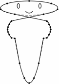
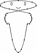
Figure 2. Left plot: Anthropomorphic shape composed of one ellipse, two hyperbolas and one parabola. The marked points refer to Table 2. Center plot: $f^{0}$, black dots. $S^{\infty}_{\epsilon}f^{0}$, solid line ($\epsilon=1$). Right plot: $f^{0}$, black dots. $T_{2,2}^{\infty}f^{0}$, solid line. The ’exact’ conic sections are represented with a dashed line in the center and right plots.

point/scheme	Ellipse	Hyperbola	Parabola
$S_{\epsilon}$	6.6613e-16	4.4755e-16	2.2204e-16
$T_{2,2}$	2.4467e-02	3.0012e-04	9.1551e-16

Table 2. Error between $S_{\epsilon}^{\infty}f^{0}$ and $T_{2,2}^{\infty}f^{0}$ and the correct value of each one of the points marked in Figure 2 left.

In addition, a non-oscillatory shape is obtained in the transition zones between two conic sections. This behavior is a distinctive feature of our scheme, when compared with its linear counterparts. For the sake of comparison, we also show $T_{2,2}^{\infty}f^{0}$ in the right plot of Figure 2. In this case, only the parabola is exactly reproduced, as confirmed by Table 2. The oscillatory behavior in the transition zones can be clearly appreciated.

9.2. Monotonicity Preservation. Smoothness of limit functions

We have proven in section 6 that monotone data is preserved by $S_{\epsilon}$ when $\epsilon\in[0,\sqrt{2}]$. If the data is strictly monotone, then this feature is also preserved. To check numerically this property, we consider as a test case the monotone data of Table 3 in [3]:

(52) $$f^{0}=(10,10,10,10,10,10.5,10.5,10.5,10.5,15,50,50,50,50,60,85,85,85,85).$$

The limit (monotone) function $S^{\infty}_{\epsilon}f^{0}$ is displayed in the left plot of Figure 3 (solid line). For the sake of comparison, $T_{2,2,}^{\infty}f^{0}$ is also shown (dotted line). The different behavior between both limit functions can be clearly appreciated in the right plot, which shows a zoom of the flat region (between jumps) marked with a rectangle on the left plot.

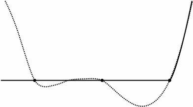
Figure 3. Left plot: $T_{2,2}^{\infty}f^{0}$ (dotted line) and $S_{\epsilon}^{\infty}f^{0}$ (solid line) with $f^{0}$ in (52). Right plot: zoom of the area marked with a dashed rectangle on the left plot.

Figure 4. Left plot: $T_{2,2}^{\infty}f^{0}$ (dotted line) and $S_{\epsilon}^{\infty}f^{0}$ (solid line) with $f^{0}$ in (53). Right plot: zoom of the area marked with a dashed rectangle on the left plot.

In section 7, we have been able to prove that when the data are strictly monotone (and appropriately chosen, see Theorem 23), the limit function is in fact $\mathcal{C}^{1}$. In order to see the possible differences between the limit functions for monotone and strictly monotone data, we slightly modify the data in (52) to have the following initial set of strictly monotone data

(53) $$f^{0}=(10,10.1,10.2,10.3,10.4,10.5,10.6,10.7,10.8,15,50,50.1,50.2,50.3,60,85,85.1,85.2,85.3).$$

In Figure 4 we display the results corresponding to $S^{\infty}_{\epsilon}f^{0}$ and $T_{2,2}^{\infty}f^{0}$, with the same convention as in Figure 3. Comparing the right plots in Figures 3 and 4, it seems evident that there is a difference in smoothness in both limit functions. To get a numerical estimate of the smoothness of the limit functions, we proceed as in [9, 17], and compute, in each case,

$$\alpha\approx\log_{2}\left(\frac{\left\|\nabla^{n}f^{k}\right\|_{\infty}}{\left\|\nabla^{n}f^{k+1}\right\|_{\infty}}\right),$$

being $n$ a natural number greater than $\alpha$. In this case, $n\geq 2$.

For the initial data in (52), we find that $\alpha\approx 1.34$. On the other hand, when $f^{0}$ is strictly monotone, as in (53), we get $\alpha\approx 2$. We have also observed (numerically) this improved smoothness in other situations, for example in reconstructing the ’heart’ shown in Figure 5, where the numerical estimate gives $\alpha\approx 2$. The right display in this figure shows a smooth reconstruction of initial ’edge’ at the bottom. Since $T_{2,2}$ is $\mathcal{C}^{2-}$ we conjecture that this is, in fact, the smoothness of the limit functions shown in Figures 4 and 5.

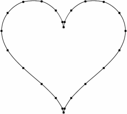
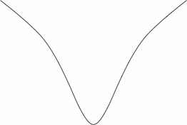
Figure 5. Left: The curve generated (line) from the initial sequence (dots) using $S_{\epsilon}$. Right: A zoom of one edge of the left figure.

Through extensive numerical testing, we have observed that the lowest regularity numerically obtained for $S^{\infty}_{\epsilon}f^{0}$, for $f^{0}$ quite arbitrary, is $\mathcal{C}^{\alpha}$, with $\alpha\approx 1.34$. In addition, this regularity seems to occur when considering four consecutive data of the form

$$f_{i-1}^{k}\leq f_{i}^{k}=f_{i+1}^{k}\leq f_{i+2}^{k}\text{ or }f_{i-1}^{k}\geq f_{i}^{k}=f_{i+1}^{k}\geq f_{i+2}^{k},$$

which is exactly the case in Figure 3. In such situations $(S_{\epsilon}f^{k})_{2i+1}=(T_{1,1}f^{k})_{2i+1}$. This choice is motivated by the desire to ensure monotonicity, but it seems to have an adverse effect on the smoothness of the limit function. In any case, we also recall that, at this moment, only $\mathcal{C}^{1}$ smoothness has been proven (under appropriate restrictions).

9.3. Approximation order

We have proven in Theorem 27 that the approximation order of $S_{\epsilon}$ after one iteration is 4, when $f=F|_{h\mathds{Z}}$ and $|F^{\prime}|>\theta>0$. For such data, we expect that stability results of section 8.2, hence we also expect that the ’strong’ approximation order is 4.

We check numerically the approximation order obtained after refining initial data sampled from the functions $F_{1}(t)=\exp(-2t^{2})$, $F_{2}(t)=\exp(t)-t$, $t_{i}^{k}=i2^{-k}/100$.

Since the approximation order depends on the monotonicity of $F$, as well as the properties of higher derivatives of $F$, we measure the error,

$$E_{k}:=\sup_{t_{i}^{k+7}\in[a,b]}\left|(S_{\epsilon}^{7}(F_{j}(t_{l}^{k}))_{l\in\mathds{Z}})_{i}-F_{j}(t_{i}^{k+7})\right|,\qquad k\geq 0,\,j=1,2.$$

at different intervals $[a,b]$, after seven applications of $S_{\epsilon}$. Notice that when $F^{\prime}$ vanishes, Theorem 27 does not apply.

	$F_{1}(t)=\exp(-2t^{2})$		$F_{2}(t)=\exp(t)-t$
$k$	$E_{k}$	$\log_{2}(E_{k}/E_{k-1})$	$E_{k}$	$\log_{2}(E_{k}/E_{k-1})$
0	5.5174e-09		6.5725e-10
1	3.4488e-10	3.9998e+00	4.1470e-11	3.9863e+00
2	2.1555e-11	4.0000e+00	2.6044e-12	3.9931e+00
3	1.3474e-12	3.9998e+00	1.6298e-13	3.9982e+00
0	3.4257e-09		4.6993e-08
1	2.1598e-10	3.9874e+00	5.8667e-09	3.0018e+00
2	1.3557e-11	3.9938e+00	7.3288e-10	3.0009e+00
3	8.4910e-13	3.9970e+00	9.1581e-11	3.0005e+00

Table 3. The error ($E_{k}$) and the approximation order ($\log_{2}(E_{k}/E_{k-1})$) of $S_{\epsilon}$ when approximating $F_{1}$ (left) and $F_{2}$ (right) after 7 iterations. The top tabular region corresponds to the monotone region $[a,b]=[-1,-0.3]$. The bottom tabular region to the non-monotone region $[a,b]=[-0.4,0.4]$.

The results are summarized in Table 3. Observe that $|F_{1}^{\prime}|,|F_{2}^{\prime}|>\theta>0$ in $[-1,-0.3]$, thus the approximation order is (shown in Table 3 top) is 4, as expected. On the other hand, $F_{1}^{\prime}(0)=0=F_{2}^{\prime}(0)$, and the approximation order is 4 and 3, respectively, in the interval $[-0.4,0.4]$ (see Table 3 bottom). To explain the difference, we may observe the Taylor expansion in the proof of Theorem 27. Different results may be expected depending on the values of $F^{\prime}(0),F^{\prime\prime}(0),F^{(3)}(0)$. Here, $0=F_{1}^{\prime\prime\prime}(0)\neq F_{1}^{\prime\prime}(0)$ and we obtained order 4, while $F_{2}^{\prime\prime}(0)\neq 0\neq F_{2}^{(3)}(0)$ and we get order 3.

which reproduces exactly third order polynomials

10. Conclusions

In [13], the authors derived non-stationary versions of the classical four point Deslauriers-Dubuc linear scheme $T_{2,2}$. These linear schemes have the capability to reproduce exactly the space of exponential polynomials $\text{span}\left\{1,t,\exp(\gamma t),\exp(-\gamma t)\right\}$, but the level-dependent rules depend explicitly on the value of the parameter $\gamma$ that defines the space. In practice, this value needs to be estimated from the initial data provided by the user. Hence, curves composed of different conic sections are hard to reproduce using these linear schemes.

In this paper, we have constructed a family of nonlinear schemes based on a nonlinear rule that can be considered as stationary representative of the linear, non-stationary 4-point schemes introduced in [13]. We show that the schemes in this family reproduce exactly second order polynomials. It also reproduces trigonometric and hyperbolic functions, provided that some easily verifiable conditions are fulfilled. We remark that no previous knowledge on the parameters defining the hyperbolic/trigonometric functions is required: the same scheme is being applied at all locations of a curve composed of different conic sections, obtaining exact reconstruction away from the transition zones between sections.

We show that the new schemes can be written as a nonlinear perturbation of a linear scheme, as in [1, 2, 3, 7, 8, 9, 16]. The analysis of convergence, monotonicity preservation and stability of the new schemes uses some of the tools developed in these references.

We remark that the proximity theory [14, 15], usually applied on manifold data subdivision schemes, cannot be applied in our case, because our schemes do not verify a proximity condition.

In addition, we have shown that, for strictly monotone data and for a certain range of the parameter that defines the cut-off function $\Gamma_{\epsilon}$, the nonlinear rules become independent of the value of this parameter, and are smooth positive functions. This allowed us to prove that the corresponding limit functions are $\mathcal{C}^{1}$ smooth, provided that a (non restrictive) technical condition is verified. Some numerical experiments were carried out to support and validate the theoretical results obtained in the paper.

The setting in this paper is one-dimensional. We plan to extend these ideas to define a new subdivision scheme, able to reproduce trigonometric functions in a bivariate setting and on triangular meshes.

Appendix A Gradient computations

This appendix describes the computation of the gradients that appear in section 7. We recall that we are assuming that the data is strictly positive and $\epsilon\in[0,\sqrt{2}]$, hence the subdivision rules of $S_{\epsilon}^{(1)}$ are

$$\Psi_{j}(x,y,z) =y+(-1)^{j}2\Gamma^{[1]}_{\epsilon}(x,y,z)(x-z),\qquad j=0,1,$$

where $\Gamma^{[1]}_{\epsilon}$, which does not depend on $\epsilon$, is given in the first row of (34).

Let us denote $\mathds{1}_{n}=(1,1,\ldots,1)\in\mathds{R}^{n}$. An easy computation leads to

$$\nabla\Psi_{j}(\mathds{1}_{3})=(0,1,0)+(-1)^{j}2\Gamma^{[1]}(\mathds{1}_{3})(1,0,-1)=(0,1,0)+(-1)^{j}\frac{1}{8}(1,0,-1).$$

Then

$$\nabla\Psi_{0}(\mathds{1}_{3})=\left(\frac{1}{8},1,-\frac{1}{8}\right),\qquad\nabla\Psi_{1}(\mathds{1}_{3})=\left(-\frac{1}{8},1,\frac{1}{8}\right).$$

Since $\Psi_{0},\Psi_{1}:\mathds{R}^{3}_{+}\rightarrow\mathds{R}$, $G_{1}$ and $G_{2}$, in (54),(55) are positive and smooth too. Hence their gradients are well-defined. Some details are provided below, and the results are summarized in Table 4. In the computations below, we use that $\Psi_{j}(\mathds{1}_{3})=1$, the chain rule and the values obtained for $\nabla\Psi_{j}(\mathds{1}_{3})$.

For $G_{1}$ we have,

(54) $$G_{1}(x,y)=\frac{\Psi_{1}(x,1,y)}{\Psi_{0}(x,1,y)}\qquad\text{for }x,y>0,\qquad\nabla(x,1,y)=\begin{pmatrix}1&0\\ 0&0\\ 0&1\end{pmatrix},$$

thus the chain rule leads to

$$\nabla G_{1}(\mathds{1}_{2}) =\frac{1}{\Psi_{0}(\mathds{1}_{3})^{2}}\left(\Psi_{0}(\mathds{1}_{3})\nabla\Psi_{1}(\mathds{1}_{3})\begin{pmatrix}1&0\\ 0&0\\ 0&1\end{pmatrix}-\Psi_{1}(\mathds{1}_{3})\nabla\Psi_{0}(\mathds{1}_{3})\begin{pmatrix}1&0\\ 0&0\\ 0&1\end{pmatrix}\right)$$

$$=\left(\left(-\frac{1}{8},1,\frac{1}{8}\right)-\left(\frac{1}{8},1,-\frac{1}{8}\right)\right)\begin{pmatrix}1&0\\ 0&0\\ 0&1\end{pmatrix}=\left(-\frac{1}{4},\frac{1}{4}\right).$$

To compute $\nabla G_{2}(\mathds{1}_{3})$, where

(55) $$G_{2}(x,y,z)=\frac{\Psi_{0}(1,y,yz)}{\Psi_{1}(x,1,y)},$$

we proceed analogously

$$\nabla G_{2}(\mathds{1}_{3})=\left(\frac{1}{8},1,-\frac{1}{8}\right)\begin{pmatrix}0&0&0\\ 0&1&0\\ 0&1&1\end{pmatrix}-\left(-\frac{1}{8},1,\frac{1}{8}\right)\begin{pmatrix}1&0&0\\ 0&0&0\\ 0&1&0\end{pmatrix}=\left(\frac{1}{8},\frac{6}{8},-\frac{1}{8}\right).$$

$$\begin{array}[]{|c|c|c|c|}\hline\cr\,\|\Psi_{0}(\mathds{1}_{3}))\|_{1}&\,\|\Psi_{1}(\mathds{1}_{3}))\|_{1}&\,\|\nabla G_{1}(\mathds{1}_{2})\|_{1}&\,\|\nabla G_{2}(\mathds{1}_{3})\|_{1}\\ \hline\cr 5/4&5/4&1/2&1\\ \hline\cr\end{array}$$

Table 4. The 1-norms of the gradients of the subdivision rules $\Psi_{0}$, $\Psi_{1}$ and the functions $G_{1}$ and $G_{2}$.

To carry out the computations required in Lemma 19, we use the following notation: The double application of $S_{\epsilon}$ is determined by

(56) $$\Psi^{2}_{j}(d_{i-2},d_{i-1},\ldots,d_{i+2}):=(S_{\epsilon}^{[1]}S_{\epsilon}^{[1]}d)_{4i+j},\quad j=0,1,2,3,4,$$

where:

$$(S_{\epsilon}^{[1]}S_{\epsilon}^{[1]}d)_{4i} =\Psi_{0}\Big{(}\Psi_{1}(d_{i-2},d_{i-1},d_{i}),\Psi_{0}(d_{i-1},d_{i},d_{i+1}),\Psi_{1}(d_{i-1},d_{i},d_{i+1})\Big{)},$$

$$(S_{\epsilon}^{[1]}S_{\epsilon}^{[1]}d)_{4i+1} =\Psi_{1}\Big{(}\Psi_{1}(d_{i-2},d_{i-1},d_{i}),\Psi_{0}(d_{i-1},d_{i},d_{i+1}),\Psi_{1}(d_{i-1},d_{i},d_{i+1})\Big{)},$$

$$(S_{\epsilon}^{[1]}S_{\epsilon}^{[1]}d)_{4i+2} =\Psi_{0}\Big{(}\Psi_{0}(d_{i-1},d_{i},d_{i+1}),\Psi_{1}(d_{i-1},d_{i},d_{i+1}),\Psi_{0}(d_{i},d_{i+1},d_{i+2})\Big{)},$$

$$(S_{\epsilon}^{[1]}S_{\epsilon}^{[1]}d)_{4i+3} =\Psi_{1}\Big{(}\Psi_{0}(d_{i-1},d_{i},d_{i+1}),\Psi_{1}(d_{i-1},d_{i},d_{i+1}),\Psi_{0}(d_{i},d_{i+1},d_{i+2})\Big{)}.$$

Applying the chain rule and the previous results, we get

$$\nabla\Psi^{2}_{0}(\mathds{1}_{5}) =(\frac{1}{8},1,-\frac{1}{8})\begin{pmatrix}-\frac{1}{8}&1&\frac{1}{8}&0&0\\ 0&\frac{1}{8}&1&-\frac{1}{8}&0\\ 0&-\frac{1}{8}&1&\frac{1}{8}&0\end{pmatrix}=(-\frac{1}{64},\frac{17}{64},\frac{57}{64},-\frac{9}{64},0),$$

$$\nabla\Psi^{2}_{1}(\mathds{1}_{5}) =(-\frac{1}{8},1,\frac{1}{8})\begin{pmatrix}-\frac{1}{8}&1&\frac{1}{8}&0&0\\ 0&\frac{1}{8}&1&-\frac{1}{8}&0\\ 0&-\frac{1}{8}&1&\frac{1}{8}&0\end{pmatrix}=(\frac{1}{64},-\frac{1}{64},\frac{71}{64},-\frac{7}{64},0),$$

$$\nabla\Psi^{2}_{2}(\mathds{1}_{5}) =(\frac{1}{8},1,-\frac{1}{8})\begin{pmatrix}0&\frac{1}{8}&1&-\frac{1}{8}&0\\ 0&-\frac{1}{8}&1&\frac{1}{8}&0\\ 0&0&\frac{1}{8}&1&-\frac{1}{8}\end{pmatrix}=(0,-\frac{7}{64},\frac{71}{64},-\frac{1}{64},\frac{1}{64}),$$

$$\nabla\Psi^{2}_{3}(\mathds{1}_{5}) =(-\frac{1}{8},1,\frac{1}{8})\begin{pmatrix}0&\frac{1}{8}&1&-\frac{1}{8}&0\\ 0&-\frac{1}{8}&1&\frac{1}{8}&0\\ 0&0&\frac{1}{8}&1&-\frac{1}{8}\end{pmatrix}=(0,-\frac{9}{64},\frac{57}{64},\frac{17}{64},-\frac{1}{64}),$$

$$\nabla\Psi^{2}_{4}(\mathds{1}_{5}) =(\frac{1}{8},1,-\frac{1}{8})\begin{pmatrix}0&-\frac{1}{8}&1&\frac{1}{8}&0\\ 0&0&\frac{1}{8}&1&-\frac{1}{8}\\ 0&0&-\frac{1}{8}&1&\frac{1}{8}\end{pmatrix}=(0,-\frac{1}{64},\frac{17}{64},\frac{57}{64},-\frac{9}{64}).$$

Then, for $j=0,1,2,3$,

(57) $$G_{j}^{2}(x,y,z,w):=\frac{\Psi^{2}_{j+1}(xy,y,1,z,zw)}{\Psi^{2}_{j}(xy,y,1,z,zw)},\qquad\nabla G_{j}^{2}(\mathds{1}_{4})=(\nabla\Psi^{2}_{j+1}(\mathds{1}_{5})-\nabla\Psi^{2}_{j}(\mathds{1}_{5}))\begin{pmatrix}1&1&0&0\\ 0&1&0&0\\ 0&0&0&0\\ 0&0&1&0\\ 0&0&1&1\\ \end{pmatrix}$$

so that

$$\nabla G^{2}_{0}(\mathds{1}_{4}) =(\frac{1}{32},-\frac{1}{4},\frac{1}{32},0), \nabla G^{2}_{2}(\mathds{1}_{4}) =(0,-\frac{1}{32},\frac{1}{4},-\frac{1}{32}),$$

$$\nabla G^{2}_{1}(\mathds{1}_{4}) =(-\frac{1}{64},-\frac{7}{64},\frac{7}{64},\frac{1}{64}), \nabla G^{2}_{3}(\mathds{1}_{4}) =(0,\frac{1}{8},-\frac{1}{2},-\frac{1}{8}).$$

The relevant results are summarized in Table 5.

$j$	0	1	2	3
$\|\nabla G^{2}_{j}(\mathds{1}_{4})\|_{1}$	5/16	1/4	5/16	3/4

Table 5. The 1-norm of the ratio functions $G^{2}_{j}$ for $j=0,1,2,3$.

References

• [1] S. Amat, K. Dadourian, and J. Liandrat. Analysis of a class of nonlinear subdivision schemes and associated multiresolution transforms. Advances in Computational Mathematics, 34(3):253–277, 2011.
• [2] Sergio Amat, Rosa Donat, Jacques Liandrat, and J Carlos Trillo. Analysis of a new nonlinear subdivision scheme. applications in image processing. Foundations of Computational Mathematics, 6(2):193–225, 2006.
• [3] F. Aràndiga, R. Donat, and M. Santágueda. The PCHIP subdivision scheme. Applied Mathematics and Computation, 272, Part 1:28 – 40, 2016. Subdivision, Geometric and Algebraic Methods, Isogeometric Analysis and Refinability.
• [4] Alfred S. Cavaretta, Charles A. Micchelli, and Wolfgang Dahmen. Stationary Subdivision. American Mathematical Society, Boston, MA, USA, 1991.
• [5] Albert Cohen, Nira Dyn, and Basarab Matei. Quasilinear subdivision schemes with applications to eno interpolation. Applied and Computational Harmonic Analysis, 15(2):89–116, 2003.
• [6] Costanza Conti and Lucia Romani. Algebraic conditions on non-stationary subdivision symbols for exponential polynomial reproduction. J. Comput. Appl. Math., 236(4):543–556, September 2011.
• [7] Karine Dadourian and Jacques Liandrat. Analysis of some bivariate non-linear interpolatory subdivision schemes. Numerical Algorithms, 48(1):261–278, 2008.
• [8] Ingrid Daubechies, Olof Runborg, and Wim Sweldens. Normal multiresolution approximation of curves. Constructive Approximation, 20(3):399–463, 2004.
• [9] Rosa Donat, Sergio López-Ureña, and Maria Santágueda. A family of non-oscillatory 6-point interpolatory subdivision schemes. Adv. Comput. Math., 2017.
• [10] David L Donoho. Interpolating wavelet transforms. Preprint, Department of Statistics, Stanford University, 2(3), 1992.
• [11] N. Dyn and D. Levin. Analysis of asymptotically equivalent binary subdivision schemes. Journal of Mathematical Analysis and Applications, 193(2):594 – 621, 1995.
• [12] Nira Dyn. Subdivision schemes in cagd. In Advances in Numerical Analysis, pages 36–104. Univ. Press, 1992.
• [13] Nira Dyn, David Levin, and Ariel Luzzatto. Exponentials reproducing subdivision schemes. Foundations of Computational Mathematics, 3(2):187–206, 2003.
• [14] Philipp Grohs. Smoothness analysis of subdivision schemes on regular grids by proximity. SIAM Journal on Numerical Analysis, 46(4):2169–2182, 2008.
• [15] Philipp Grohs. A general proximity analysis of nonlinear subdivision schemes. SIAM Journal on Mathematical Analysis, 42(2):729–750, 2010.
• [16] S. Harizanov and P. Oswald. Stability of nonlinear subdivision and multiscale transforms. Constructive Approximation, 31(3):359–393, 2010.
• [17] Frans Kuijt. Convexity preserving interpolation - stationary nonlinear subdivision and splines. PhD thesis, Enschede, October 1998.
• [18] Amos Ron. Exponential box splines. Constructive Approximation, 4(1):357–378, 1988.