Constraint Energy Minimizing Generalized Multiscale Finite Element Method for high-contrast linear elasticity problem

Abstract

In this paper, we consider the offline and online Constraint Energy Minimizing Generalized Multiscale Finite Element Method (CEM-GMsFEM) for high-contrast linear elasticity problem. Offline basis construction starts with an auxiliary multiscale space by solving local spectral problems. We select eigenfunctions that correspond to a few small eigenvalues to form the auxiliary space. Using the auxiliary space, we solve a constraint energy minimization problem to construct offline multiscale spaces. The minimization problem is defined in the oversampling domain, which is larger than the target coarse block. To get a good approximation space, the oversampling domain should be large enough. We also propose a relaxed minimization problem to construct multiscale basis functions, which will yield more accurate and robust solution. To take into account the influence of input parameters, such as source terms, we propose the construction of online multiscale basis and an adaptive enrichment algorithm. We provide extensive numerical experiments on 2D and 3D models to show the performance of the proposed method.

1 Introduction

In many science and engineer problems, one encounters multiple scales and high contrast. For example, wave propagation in fractured media, immiscible flow processes in poroelastic media and so on. Due to the advancement of media characterization methods and geostatistical modeling techniques, the media can be detailed at very fine scales, as a result, one needs to solve huge dimensional algebraic systems. Therefore, model reduction methods are proposed by researchers to reduce the problem size and alleviate the computational cost. Typical model reduction techniques include upscaling and multiscale methods. In upscaling methods [19, 11, 15], one typically upscales the media properties based on the homogenization theory so that the problem can be solved on a coarse grid. In multiscale methods [12, 13, 5, 4, 17, 18, 1, 20, 16], one still solves the problems on a coarse grid but with precomputed media dependent multiscale basis functions.

Among above mentioned multiscale methods, the multiscale finite element method (MsFEM) [16, 13] is a classic multiscale method that has shown great success in various practical applications. However, the MsFEM assumes that the media is scale separable. To overcome this assumption, the generalized multiscale finite element method (GMsFEM)[14] was proposed. The GMsFEM provide a systematic way to construct multiple multiscale basis. In particular in GMsFEM, one first creates an appropriate snapshot space and then solve a carefully designed local spectral problem in snapshot space. The basis space are filled with the dominant eigenvectors corresponding to small eigenvalues. The GMsFEM’s convergence depends on decay behavior of the eigenvalues of the local spectral problems [14]. In [8], the authors applied the GMsFEM to solve the linear elasticity problem in high contrast problem, they consider both the continuous and discontinuous Galerkin method to couple the multiscale basis functions. In this paper, we will extend the recently proposed constraint energy minimizing GMsFEM (CEM-GMsFEM)[9] for high contrast linear elasticity problem. The CEM-GMsFEM consists of two steps. One needs to first construct auxiliary basis functions by solving local spectral problems. Then, for each auxiliary basis function, one can construct a multiscale basis via energy minimization problems on subdomains. We propose two versions . The first one is based on solving constraint energy minimization problems and the second one is the relax version by solving unconstrained energy minimization problems. The convergence of the CEM-GMsFEM not only depends on the eigenvalue but also depends on the coarse mesh size when the oversampling domain is carefully chosen.

To incorporate the influence of source and global media information, we also propose the construction of online multiscale basis. The idea of online approach was first proposed in [6] and has been extended to various other cases (see [7, 3, 21]). The key idea is using the residual information of the coarse-grid solution to construct multiscale basis. These online multiscale basis functions can also be computed adaptively so that the error can be decreased the most. The online basis of CEM-GMsFEM [10] will be computed in a oversampled domain, which is different from the original online approach [6]. We test our methods on 2D and 3D media with channels and inclusions. By properly selecting the number of basis functions and oversampling layers, we can observe that the multiscale solution can approximate the fine-scale solution accurately.

This paper will be organized as follows. In Section 2, we will present some preliminaries. In Section 3, the construction of offline multiscale basis functions of CEM-GMsFEM is discussed. In Section 4, we present a online adaptive enrichment algorithm. In Section 5, we provide some convergence results. In Section 6, a few numerical results are presented to demonstrate the performance of the method. Finally, some conclusions are given.

2 Preliminaries

We consider isotropic linear elasticity problem in heterogeneous media as:

$$-\nabla\cdot{\sigma(u)}={f},\quad\text{ in }\;D$$ (1)

where $D\subset\mathbb{R}^{d}(d=2,3)$ be a bounded domain representing the elastic body of interest, $u$ is the vector displacement field, ${\sigma}({u})$ is the stress tensor and it is related to the strain tensor ${\epsilon}({u})$ in the following way

$${\sigma(u)}=2\mu{\epsilon(u)}+\lambda\nabla\cdot{u}\,{\mathcal{I}},$$

where $\lambda>0$ and $\mu>0$ are the Lamé coefficients and can be highly heterogeneous, $\mathcal{I}$ is the identity tensor. The strain tensor ${\epsilon}({u})=(\epsilon_{ij}({u}))_{1\leq i,j\leq d}$ is defined by

$${\epsilon}({u})=\frac{1}{2}(\nabla{u}+\nabla{u}^{T}),$$

where $\displaystyle\nabla{u}=(\frac{\partial u_{i}}{\partial x_{j}})_{1\leq i,j\leq d}$. In the component form, we have

$$\epsilon_{ij}({u})=\frac{1}{2}\Big{(}\frac{\partial u_{i}}{\partial x_{j}}+\frac{\partial u_{j}}{\partial x_{i}}\Big{)},\quad 1\leq i,j\leq d.$$

For simplicity, we will consider the homogeneous Dirichlet boundary condition ${u}={0}$ on $\partial D$. Other types of boundary conditions can be taken care easily in the way used in classical approaches.

Let $\mathcal{T}^{H}$ be a conforming partition of the domain $D$. We call $\mathcal{T}^{H}$ the coarse grid and $H$ the coarse mesh size. Each element of $\mathcal{T}^{H}$ is called a coarse grid block. Denote $N_{c}$ be the total number of vertices of $\mathcal{T}^{H}$ and $N$ be the total number of coarse blocks. Let $\{x_{i}\}_{i=1}^{Nc}$ be the set of vertices in $\mathcal{T}^{H}$ and $\omega_{i}=\cup\{K_{j}\in\mathcal{T}^{H}|x_{i}\in\overline{K_{j}}\}$. In addition, we let $\mathcal{T}^{h}$ be a conforming refinement of the triangulation $\mathcal{T}^{H}$. We call $\mathcal{T}^{h}$ the fine grid and $h>0$ is the fine mesh size. Figure 1 shows an illustration of the fine scale grid, coarse scale grid, and oversampling domain.

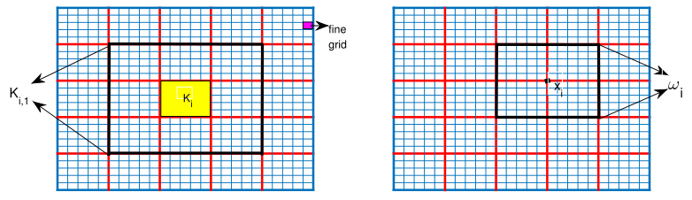
Figure 1: Illustration of the coarse grid, fine grid, oversampling domain $K_{i,1}$ and neighborhood.

Let $V=H_{0}^{1}(D)$, then the solution $u$ to (1) satisfies

$$a({u},{v})=({f},{v}),\quad\forall{v}\in V,$$ (2)

where

$$a({u},{v})=\int_{D}\Big{(}2\mu{\epsilon}({u}):{\epsilon}({v})+\lambda\nabla\cdot{u}\,\nabla\cdot{v}\Big{)}\;d{x},\quad({f},{v})=\int_{D}{f}\cdot{v}\;d{x}$$ (3)

and

$${\epsilon}({u}):{\epsilon}({v})=\sum_{i,j=1}^{d}\epsilon_{ij}({u})\epsilon_{ij}({v}),\quad{f}\cdot{v}=\sum_{i=1}^{d}f_{i}v_{i}.$$ (4)

We will construct multiscale space $V_{ms}\subset V$ and obtain the solution in $V_{ms}$. That is, find $u_{ms}\in V_{ms}$ such that

$$a(u_{ms},v)=(f,v),\quad\forall{v}\in V_{ms},$$ (5)

To evaluate the accuracy of multiscale solution $u_{ms}$, we will compute the solution of (2) on fine grid $\mathcal{T}_{h}$, denoted by $u_{h}$ which is fine enough to resolve all the heterogeneities of the exact $u$. Let $V_{h}$ be the first-order Galerkin finite element basis space with respect to the fine grid $\mathcal{T}_{h}$, and $q_{1},\cdots,q_{n}$ be the basis set for $V_{h}$, then $u_{h}$ satisfies $A_{h}u_{h}=F_{h}$, where $A_{h}$ is a symmetric, positive definite matrix with $A_{h,ij}=a(q_{j},q_{i})$, $F_{h}$ is a vector whose $i$-th component is $(f,q_{i})$. We will also use first order finite element on fine grid $\mathcal{T}_{h}$ to compute the multiscale basis functions numerically. Then each multiscale basis function can be treated as a column vector $\Phi_{i}$, let $R=[\Phi_{1},\cdots,\Phi_{Nms}]$ be the matrix that stores all the multiscale basis functions (total number is $Nms$), then the multiscale solution satisfies $u_{ms}=(R^{T}A_{h}R)^{-1}(R^{T}F_{h})$, one can also project the coarse solution $u_{ms}$ into space $V_{h}$ by $u_{ms}^{f}=Ru_{ms}$.

3 The construction of the CEM-GMsFEM basis functions.

This section is devoted to the construction of the multiscale basis functions. There are two stages, the first stage is to construct the auxiliary multiscale basis function with the concept of generalized multiscale finite element method (GMsFEM). Then, we can construct the multiscale basis function by solving some energy minimizing problems in the oversampling domain.

3.1 Auxiliary basis functions

The auxiliary multiscale basis functions are constructed by solving a spectral problem in each coarse block $K_{i}$. More specifically, for each coarse block $K_{i}$, we let $V(K_{i})$ be the restriction of $V$ on $K_{i}$, then we solve the spectral problem: find $(\lambda_{j}^{i},\phi_{j}^{i})\in\mathbb{R}\times V(K_{i})$

$$a_{i}(\phi_{j}^{i},v)=\lambda_{j}^{i}s_{i}(\phi_{j}^{i},v),\quad\forall v\in V(K_{i})$$

where $a_{i}(u,v)=\int_{K_{i}}2\mu{\epsilon}({u}):{\epsilon}({v})+\lambda\nabla\cdot{u}\,\nabla\cdot{v}$, $s_{i}(u,v)=\int_{K_{i}}\tilde{\kappa}uv$, $\tilde{\kappa}=\sum_{i=1}^{N_{c}}(\lambda+2\mu)|\nabla\chi_{i}|^{2}$ and ${\chi_{i}}$ is a set of partition of unity functions (see[2]) on the coarse grid. We choose $J_{i}$ eigenfunctions corresponding to first $J_{i}$ smallest eigenvalues to form the local auxiliary space $V_{\text{aux}}(K_{i})$, which is

$$V_{\text{aux}}(K_{i})=\text{span}\{\phi_{j}^{i}|1\leq j\leq J_{i}\}.$$

We can normalize these eigenfunctions such that $s_{i}(\phi_{j}^{i},\phi_{j}^{i})=1$, we also denote $\Lambda$ as the minimum first discarded eigenvalue. Then, the auxiliary space $V_{\text{aux}}$ is defined as the sum of all local auxiliary spaces $V_{\text{aux}}(K_{i})$. We define the notion of $\phi$-orthogonality in the space V. That is given a function $\phi_{j}^{i}\in V_{\text{aux}}$, we say that a function $\psi\in V$ is $\phi_{j}^{i}$-orthogonal if

$$s(\psi,\phi_{j}^{i})=1,\quad s(\psi,\phi_{j^{\prime}}^{i^{\prime}})=0\quad\text{if }j^{\prime}\neq j\text{ or }i^{\prime}\neq i.$$

where $s(u,v)=\sum_{i=1}^{N}s_{i}(u,v)$. We also define a projection operator $\pi$ from space $V$ to $V_{\text{aux}}$ by

$$\pi(v)=\sum_{i=1}^{N}\sum_{j=1}^{J_{i}}s_{i}(v,\phi_{j}^{i})\phi_{j}^{i},\quad\forall v\in V,$$

The kernel of the operator $\pi$ can be defined as

$$\tilde{V}=\{w\in V|\pi(w)=0\}.$$

3.2 Offline multiscale basis functions

With the auxiliary space, we can introduce the construction of offline multiscale basis functions. For each coarse block $K_{i}$, we can extend this region by $m$ coarse grid layer and obtain an oversampled region $K_{i,m}$ (see Figure 1 for an example of $K_{i,1}$). Then for each auxiliary function $\phi_{j}^{i}\in V_{\text{aux}}$, the multiscale basis function $\psi_{j,ms}^{i}$ can be defined by

$$\psi_{j,ms}^{i}=\text{argmin}\Big{\{}a(\psi,\psi)|\psi\in V_{0}(K_{i,m}),\psi\text{ is }\phi_{j}^{i}\text{-orthogonal}\Big{\}}.$$ (6)

where $V_{0}(K_{i,m})=H_{0}^{1}(K_{i,m})$. By using Lagrange Multiplier, the problem (6) can be rewritten as the following problem: find $\psi_{j,ms}^{i}\in V_{0}(K_{i,m}),$ $\lambda\in V_{\text{aux}}^{i}$ such that

$$\begin{split}a(\psi_{j,ms}^{i},p)+s(p,\lambda)&=0\quad\forall p\in V_{0}(K_{i,m}),\\ s(\psi_{j,ms}^{i}-\phi_{j}^{i},q)&=0\quad\forall q\in V_{\text{aux}}^{i}(K_{i,m}),\end{split}$$ (7)

where $V_{\text{aux}}^{i}(K_{i,m})$ is the union of all local auxiliary spaces for $K_{j}\subset K_{i,m}$. One can numerically solve above continuous problem with fine scale mesh. More specifically, denote $M_{h}$ be the matrix such that $M_{h,ij}=s(q_{j},q_{i})$, $A_{h}^{i}$and $M_{h}^{i}$ be the restriction of $A_{h}$ and $M_{h}$ on $K_{i,m}$ respectively. $P^{i}$ is the matrix that includes all the discrete auxiliary basis in space $V_{\text{aux}}(K_{i,m})$.

The matrix formulation of problem (7) is

$$\left[\begin{array}[]{cc}A_{h}^{i}&M_{h}^{i}P^{i}\\ (M_{h}^{i}P^{i})^{T}&0\\ \end{array}\right]\left[\begin{array}[]{cc}\psi_{h}^{i}\\ \lambda_{h}^{i}\end{array}\right]=\left[\begin{array}[]{cc}0\\ I_{i}\end{array}\right]$$ (8)

where $P^{i}_{j}$ is the $j$-th column of $P^{i}$, $\psi_{j,h}^{i}$ is discrete $\psi_{j,ms}^{i}$, $I_{i}$ is a sparse matrix whose nonzero elements (all are 1) are in the diagonal of the matrix, the position of these nonzero elements depends on the index order of $K_{i}$ in $K_{i,m}$.

Following [9], we can relax the $\phi$-orthogonality in (6) and get a relaxed version of the multiscale basis functions. More specifically, we solve the following un-constrainted minimization problem: find $\psi_{j,ms}^{i}\in V_{0}(K_{i,m})$ such that

$$\psi_{j,ms}^{i}=\text{argmin}\Big{\{}a(\psi,\psi)+s(\pi\psi-\phi_{j}^{i},\pi\psi-\phi_{j}^{i})|\psi\in V_{0}(K_{i,m})\Big{\}}.$$ (9)

which is equivalent to the following local problem

$$a(\psi_{j,ms}^{i},v)+s(\pi(\psi_{j,ms}^{i}),\pi(v))=s(\phi_{j}^{i},\pi(v)),\quad\forall v\in V_{0}(K_{i,m}).$$ (10)

Using above defined notation, then the matrix formulation of Equation (10) is

$$\left(A_{h}^{i}+M_{h}^{i}(P^{i}P^{i,T})M_{h}^{i,T}\right)\psi_{j,h}^{i}=P^{i}_{j}M_{h}^{i,T}$$ (11)

For each auxiliary basis $\phi_{j}^{i}$, one can get a multiscale basis $\psi^{i}_{j,ms}$. The final multiscale basis function space $V_{ms}$ is the span of all multiscale basis functions. Since the construction of the multiscale basis includes solving spectral problems and energy minimization problems, therefore we call this method the CEM-GMsFEM. Figure 2 shows an example of relaxed CEM-GMsFEM basis functions, it can be observed that the multiscale basis concentrated on the support of auxiliary basis function and decays outside the support. The multiscale basis functions can be treated as an approximation to global multiscale basis function $\psi_{j}^{i}\in V$ which is defined in a similar way, namely,

$$\psi_{j}^{i}=\text{argmin}\Big{\{}a(\psi,\psi)|\psi\in V,\psi\text{ is }\phi_{j}^{i}\text{-orthogonal}\Big{\}}.$$ (12)

for the constraint case and

$$\psi_{j}^{i}=\text{argmin}\Big{\{}a(\psi,\psi)+s(\pi\psi-\phi_{j}^{i},\pi\psi-\phi_{j}^{i})|\psi\in V\Big{\}}.$$ (13)

for the relaxed case. Then we can define the global space by $V_{glo}=\text{span}\{\psi_{j}^{i}\}$, this global basis functions decays exponential (see[9]) and it is important to the convergence analysis.

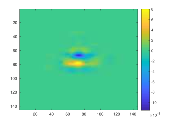
(a) First mulitscale basis

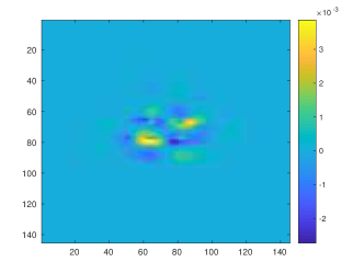
(b) Second mulitscale basis

Figure 2: Example of relaxed CEM-GMsFEM basis functions.

4 Online multiscale basis functions and adaptive enrichment

In this subsection, we present the construction of online multiscale basis functions and an adaptive enrichment algorithm based on an error estimate. Different with the offline basis, the online basis functions are constructed iteratively using the residual of previous multiscale solution, therefore it contains the source information and global information of the media.

Let $u_{ms}\in V$ be the multiscale solution of (5). Then, we can define a residual functional $r:V\to\mathbb{R}$ by

$$r(v)=a(u_{ms},v)-\int_{D}fv,\quad\forall v\in V.$$ (14)

The discrete residual in matrix form is $F_{h}-A_{h}\big{(}R((R^{T}A_{h}R)^{-1}(R^{T}F_{h}))\big{)}$. For each neighborhood $\omega_{i}$ (see Figure 1), we can define the local residual functional $r_{i}:V\to\mathbb{R}$ by

$$r_{i}(v)=r(\chi_{i}v),\quad\forall v\in V.$$ (15)

. The residual functional provides a way to measure the error $u-u_{ms}$ in $D$ and $\omega_{i}$. Then, we can construction online basis function whose support is an oversampled region $\omega_{i}^{+}$ with the local residual $r_{i}$. More specifically, the online basis function $\beta_{ms}^{i}$ satisfies following equation:

$$a(\beta_{ms}^{i},v)+s(\pi(\beta_{ms}^{i}),\pi(v))=r_{i}(v),\quad\forall v\in H_{0}^{1}(\omega_{i}^{+}),$$ (16)

Solving Equation (16) is similar with solving Equation (10). The online multiscale basis function is also localization results of corresponding global online basis function $\beta_{glo}^{i}\in V$ defined by

$$a(\beta_{ms}^{i},v)+s(\pi(\beta_{ms}^{i}),\pi(v))=r_{i}(v),\quad\forall v\in V.$$ (17)

In practice, we can adaptively compute online basis for selected neighborhoods (with $i\in I$ for an index set I). After we construct the online basis functions, we can enrich the offline multiscale basis space by adding the online basis, namely, $v_{ms}=V_{ms}+\text{span}_{i\in I}\{\beta_{ms}^{i}\}$. With the new multiscale basis function space, we can compute new multiscale solution and new basis space. These steps can be repeated until the residual norm is smaller than a given tolerance. Before presenting the algorithm, we first define the $a$-norm $||\cdot||_{a}$ where $||u||_{a}^{2}=a({u},{u})$. Next, we present the online adaptive enrichment algorithm.
Online adaptive enrichment algorithm

We first construct the offline basis functions space $V_{ms}^{0}$ introduced in Section 3. We also choose a real parameter $\theta$ such that $0\leq\theta\leq 1$ to determine the number of online basis functions added in each online iteration. Then for $m=0,1,2,\cdots$, we assume that $V_{ms}^{m}$ is already obtained, then the updated multiscale basis functions space $V_{ms}^{m+1}$.
Step 1: Find the multiscale in the current space $V_{ms}^{m}$. That is to find $u_{ms}^{m}\in V_{ms}^{m}$ such that

$$a(u_{ms}^{m},v)=(f,v),\quad\text{for all }v\in V_{ms}^{m}.$$

Step 2: For each neighborhood $\omega_{i}$, we compute the residual $z_{i}(v)$ by

$$z_{i}(v)=a(u_{ms}^{m},v)-(f,v),\quad\forall v\in V_{0}(\omega_{i}).$$

Denote $\delta_{i}=||z_{i}||_{a^{*}}=\text{sup}_{v\in V_{0}(\omega_{i})}\frac{r(v)}{||v||_{a}}$. We rearrange the order of $\omega_{i}$ such that $\delta_{1}\geq\delta_{2}\cdots.$ Then we choose the first $k$ neighborhoods such that

$$\sum_{i=k+1}^{N}\leq\theta_{i}^{2}\sum_{i=1}^{N}\delta_{i}^{2}$$

Step 3: Compute the local online basis functions in selected $k$ neighborhoods. For each $1\leq i\leq k$ and neighborhood $\omega$, we find $\beta_{ms}^{i}\in V_{0}(\omega_{i}^{+})$ satisfies

$$a(\beta_{ms}^{i},v)+s(\pi(\beta_{ms}^{i}),\pi(v))=r_{i}^{m}(v)\quad\forall v\in V_{0}(\omega_{i}^{+}),$$

where $r_{i}^{m}(v)=a(u_{ms}^{m},\chi_{i}v)-\int_{D}f\chi_{i}v$
Step 4: Update the multiscale basis function space. That is form $V_{ms}^{m+1}$ by

$$V_{ms}^{m+1}=V_{ms}^{m}+\text{span}_{1\leq i\leq k}{\beta_{ms}^{i}}.$$

5 Convergence results

In this section, we provide convergence results without giving the details of the analysis since it is quite similar with the techniques used in [10, 9]. We define $s$-norm $||\cdot||_{s}$ by $||u||_{s}^{2}=\int_{D}\tilde{k}u^{2}$. We have following three theorems.

Theorem 1.

Let $u$ be the solution of equation (2) and $u_{ms}^{\text{off}}$ be the multiscale solution of (5), the multiscale basis is the constraint case. Then we have

$$||u-u_{ms}^{\text{off}}||_{a}\leq C\Lambda^{-\frac{1}{2}}||\tilde{k}^{-\frac{1}{2}}f||_{L^{2}(D)}+C(k+1)^{\frac{d}{2}}E^{\frac{1}{2}}||u_{glo}||_{s}$$ (18)

where $E$ is a constant that depends on $\Lambda$ and $m$, $u_{glo}$ is the multiscale solution using corresponding global basis.

Theorem 2.

Let $u$ be the solution of equation (2) and $u_{ms}^{\text{off}}$ be the multiscale solution of (5), the multiscale basis is the relaxed case. Then we have

$$||u-u_{ms}^{\text{off}}||_{a}\leq C\Lambda^{-\frac{1}{2}}||\tilde{k}^{-\frac{1}{2}}f||_{L^{2}(D)}+C(k+1)^{\frac{d}{2}}E^{\frac{1}{2}}(1+D)^{\frac{1}{2}}||u_{glo}||_{s}$$ (19)

where $E$ and $D$ are constants that depend on $\Lambda$ and $m$, $u_{glo}$ is the multiscale solution using corresponding global basis.

Theorem 3.

Let $u$ be the solution of equation (2) and $u_{ms}^{l}$ be the sequence of multiscale solutions generated by the online adaptive enrichment algorithm, the offline multiscale basis is the relaxed case Then we have

$$||u-u_{ms}^{l+1}||_{a}^{2}\leq 3(1+\Lambda^{-1})\big{(}C(m+1)^{d}E+2M^{2}\theta\big{)}||u-u_{ms}^{l}||_{a}^{2}$$

where $E=3(1+\Lambda^{-1})(1+2(1+\Lambda^{\frac{1}{2}})^{-1})^{1-m}$, $M$ is maximum number of overlapping subdomains and $C$ is a constant.

6 Numerical results

In this section, we present several numerical experiments to show the performance of our method. The computational domain $D:=(0,1)^{d}$, we use constant force. We consider two high-contrast models whose Young’s modulus $E(x)$ are depicted in Figure 3. As it is shown, both models contain high conductivity channels and isolated inclusions. We note that for model 1, $E(x)=1$ in the blue region and $E(x)=E_{1}$ in the yellow region, while for model 2, $E(x)=1$ in the blank region and $E(x)=E_{2}$ in the red region. $\lambda(x)=\frac{\nu}{(1+2\nu)(1-\nu)}E(x),\mu(x)=\frac{1}{2(1+\nu)}E(x),$ the Poisson ration $\nu$ is $0.2$, both $E_{1}$ and $E_{2}$ equal $10^{4}$ unless specifically illustrated. The resolution of model 1 is $256\times 256$, while for model 2 the resolution is $64\times 64\times 64.$ For all numerical results reported below, we use "$n_{\text{ov}}$" to represent the number of oversampling coarse layers used to compute the multiscale basis, "$N_{b}$" is the number of basis used per coarse region, "Dof" means the degree of freedom of the resulting algebraic system, "$H$" is the coarse grid size. To quantify the accuracy of CEM-GMsFEM, we define relative weighted $L^{2}$ norm error and weighted $H^{1}$ norm error as follows:

$$e_{L^{2}}=\frac{||(\lambda+2\mu)(u_{ms}-u_{h})||_{L^{2}(D)}}{||(\lambda+2\mu)u_{h}||_{L^{2}(D)}},\quad e_{H^{1}}=\sqrt{\frac{a(u_{ms}-u_{h},u_{ms}-u_{h})}{a(u_{h},u_{h})}}$$

where $u_{h}$ is the fine-grid first order FEM solution. We first summarize our observations:

• CEM-GMsFEM solution converges $H$ converges to 0 as $H$ converges to 0 for both relaxed and constraint case

• Relaxed CEM-GMsFEM is more accurate and robust than constraint CEM-GMsFEM under the same parameter setting

• Using more basis functions, adding mode oversampling coarse layers can improve the CEM-GMsFEM solution

• Online basis can accelerate the convergence of the CEM-GMsFEM solution.

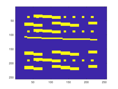
(a) Model 1

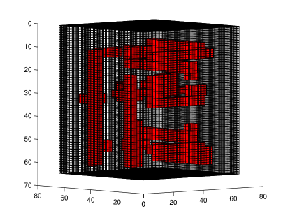
(b) Model 2

Figure 3: Young’s modulus.

6.1 Constraint CEM-GMsFEM for model 1

We first present the test results of constraint CEM-GMsFEM on model 1. The convergence history with various coarse mesh sizes $H$ are shown in Table 1 and Table 2. For the simulation results reported in Table 1, we take the number of oversampling layer to be approximately $3\text{log}(H)/\text{log}(1/8)$, as we can see, although the coarse solution converges as $H$ decreases, however the accuracy is not satisfiable, the $L^{2}$ error decrease from $68\%$ to only $26\%$. Therefore we increase the number of oversampling layer to approximately $4\text{log}(H)/\text{log}(1/8)$, the corresponding results are reported in Table 2. We find that both the $L^{2}$ and $H^{1}$ error improve a lot, and the errors decay also become faster. We emphasize that, in these simulations, we use 4 basis functions per coarse block since the eigenvalue problem on each coarse block has 4 small eigenvalues, and we need to include the first 4 eigenfunctions in the auxiliary space based on our theory. We also test the influence of number of basis, the results are presented in Figure 4. It can be seen clearly that increasing the number of basis will increase the accuracy of the CEM-GMsFEM solution. By varying the number of the oversampling coarse layers, we get results shown in Figure 5. We observe that the size of the subdomain to compute multiscale basis is quite important to the accuracy of CEM-GMsFEM, using more oversampling coarse layers will definite lead to more accurate coarse solution, this agrees with the observations from Table 1 and 2. However, after the number of oversampling layers exceeds a certain number, the errors decay become slower. We also test different contrast case with fixed oversampling layer and number of basis functions, the relative $H^{1}$ error is shown in Table 3, we find that the performance of the scheme will deteriorate as the medium contrast increases, which is predicted by theoretical analysis. This motivates the propose of relaxed CEM-GMsFEM.

$N_{b}$	$H$	$n_{\text{ov}}$	$e_{L^{2}}$	$e_{H^{1}}$
4	1/8	3	6.77e-01	7.87e-01
4	1/16	4	4.80e-01	6.28e-01
4	1/32	5	3.70e-01	5.23e-01
4	1/64	6	2.62e-01	4.40e-01

Table 1: Numerical results with varying coarse grid size $H$ for the test model 1, constraint case.

$N_{b}$	$H$	$n_{\text{ov}}$	$e_{L^{2}}$	$e_{H^{1}}$
4	1/8	4	5.65e-02	2.35e-01
4	1/16	5	2.73e-02	1.50e-01
4	1/32	7	4.47e-03	5.57e-02
4	1/64	8	2.67e-03	4.27e-02

Table 2: Numerical results with varying coarse grid size $H$ for the test model 1, constraint case.

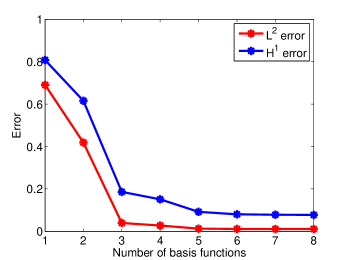
Figure 4: Numerical results with different numbers of basis functions, $H=1/16$, $n_{\text{ov}}=5$, constraint case.

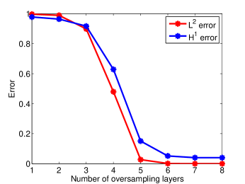
Figure 5: Numerical results with different numbers of oversampling layers, $H=1/16$, $N_{b}=4$, constraint case.

$10^{2}$ $10^{4}$ $10^{6}$ $10^{8}$ $10^{10}$ 5 1.90e-02 8.04e-02 4.04e-01 6.94e-01 7.18e-01 6 1.47e-02 2.38e-02 1.33e-01 5.19e-01 7.10e-01 7 1.45e-02 1.93e-02 3.43e-02 2.31e-01 6.07e-01

Table 3: Comparison ($e_{H^{1}}$) of various number of oversampling layers and different contrast values for test model 1, constraint case, $H=1/16,N_{b}=6$.

6.2 Relaxed CEM-GMsFEM for model 1

In this subsection, we present the performance of Relaxed CEM-GMsFEM for model 1. We first linearly decrease the coarse-grid size and the results are shown in Table 4. We observe that the coarse solution converge fast as $H$ decreases, for example , the $L^{2}$ error decays from $9\%$ to $0.0006\%$. The $L^{2}$ error convergence faster (close to second order) than the energy error (close to first order). By comparing to the similar test case in Table 1 and 2, we see that the relaxed version needs fewer oversampling layers and obtains much better results. Figure 6 shows the displacement fields of the reference solution, we can see complicated multiscale behavior of the solution. Figure 7 is the CEM-GMsFEM solution, we see the coarse solution can capture almost all the details of the reference solution and there is almost no difference with the reference solution. We also investigate the performance with different number of eigenfunctions in the auxiliary space and number of oversampling layers, the results are reported in Figure 8 and Figure 9. Again, as predicted by the theory, using more basis and larger subregion size will improve the accuracy of the CEM-GMsFEM solution. The results of robustness test are shown in Table 5, we can see that the relaxed CEM-GMsFEM is more robust with respect to the contrast.

$N_{b}$	$H$	$n_{\text{ov}}$	$e_{L^{2}}$	$e_{H^{1}}$
4	1/8	3	9.04e-02	2.72e-01
4	1/16	4	1.35e-04	4.63e-02
4	1/32	5	2.20e-05	1.47e-02
4	1/64	6	5.92e-06	4.01e-03

Table 4: Numerical results with varying coarse grid size $H$ for the test model 1, relaxed case.

(a) First component

(b) Second component

Figure 6: Reference solution

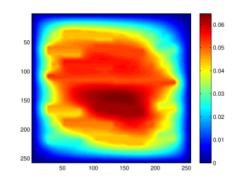
(a) First component

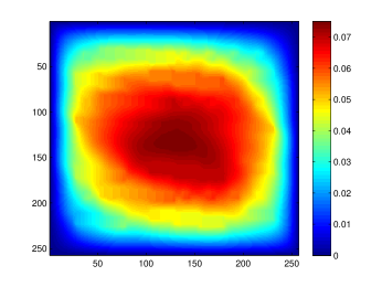
(b) Second component

Figure 7: Relaxed CEM-GMsFEM solution, $N_{b}$=4, H$=1/16$, $n_{\text{ov}}=4$.

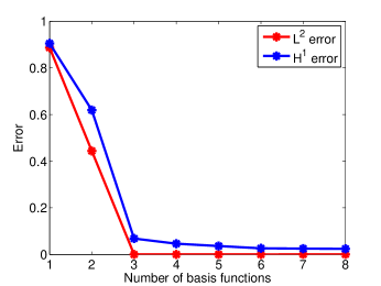
Figure 8: Numerical results with different numbers of basis functions, $H=1/16$, $n_{\text{ov}}=4$, relaxed case.

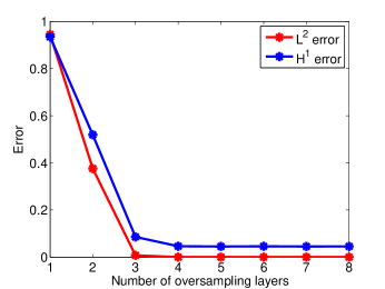
Figure 9: Numerical results with different numbers of oversampling layers, $H=1/16$, $N_{b}=4$, relaxed case.

$10^{2}$ $10^{4}$ $10^{6}$ $10^{8}$ $10^{10}$ 5 1.98e-02 2.25e-02 2.36e-02 4.59e-02 3.00e-01 6 2.00e-02 2.26e-02 2.35e-02 2.33e-02 4.32e-02 7 1.97e-02 2.25e-02 2.26e-02 2.34e-02 2.35e-02

Table 5: Comparison ($e_{H^{1}}$) of various number of oversampling layers and different contrast values for test model 1 , constraint case, relaxed case, $H=1/16,N_{b}=6$.

We also test the online iterative algorithm, the results are reported in Table 6 and Table 7. We can see that with online basis functions, the convergence is very fast. Table 6 shows the results of uniform enrichment, by comparing it with Table 7, we conclude that adaptive enrichment is better especially in reducing the $L^{2}$ error.

Dof	$n_{\text{ov}}$	$e_{L^{2}}$	$e_{H^{1}}$
16384	4	1.55e-02	1.02e-01
20353	4	2.91e-05	5.10e-03
24322	4	3.54e-07	3.88e-04

Table 6: Uniform enrichment error decay history for the test model 1, $H=1/64$, 4 offline basis used.

Dof	$n_{\text{ov}}$	$e_{L^{2}}$	$e_{H^{1}}$
16384	4	1.55e-02	1.02e-01
17112	4	9.25e-05	9.11e-03
17837	4	1.29e-05	3.91e-03
18574	4	1.02e-05	3.45e-03

Table 7: Adaptive enrichment with $\theta=0.1$ error decay history for the test model 1, $H=1/64$, 4 offline basis used.

6.3 Relaxed CEM-GMsFEM for model 2

In subsection, we present the test results of relaxed CEM-GMsFEM on model 2. We consider using a oversampling layer of $2\text{log}(H)/\text{log}(1/8)$ and 8 eigenfunction in local auxiliary basis space. The results with varying coarse grid size and fixed $N_{b}$ are shown in Table 8. We also observe that multiscale solution converges with respect to the coarse grid size. Figure 10 and Figure 11 show the displacement fields comparison between the reference solution and multiscale solution, we can see that multiscale solution can approximate the reference solution pretty well. We also consider using different number of auxiliary basis functions, the results are shown in Figure 12. Again we find that using more basis will increase the accuracy of the coarse solution. Once the basis number reaches a value, the decay of the error becomes slower. By varying the contrast of the media, we obtain various results shown in Table 9. We find that increasing the number of oversampling layers can increase robustness of the method. The uniform and adaptive online convergence history are presented in Table 10 and 11 respectively, we can observe a fast decay of the error with more basis used, adaptive enrichment is better than the uniform enrichment in reducing the $L^{2}$ error. The reason that why uniform is better in reducing $H^{1}$ error is that using uniform number of basis functions may yield the more smoother solution than non-uniform case, the relative errors are more uniform in different regions. From the results shown in Table 11 and Figure 12, we can observe the superiority of the online basis.

$N_{b}$	$H$	$n_{\text{ov}}$	$e_{L^{2}}$	$e_{H^{1}}$
8	1/8	2	1.73e-01	3.08e-01
8	1/16	3	2.15e-02	1.10e-01

Table 8: Numerical results with varying coarse grid size $H$ for the test model 2, relaxed case.

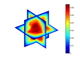
(a) First component

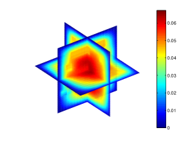
(b) First component

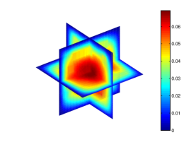
(c) Third component

Figure 10: Reference solution

(a) First component

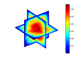
(b) First component

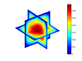
(c) Third component

Figure 11: Relaxed CEM-GMsFEM solution, $N_{b}$=8, H$=1/16$, $n_{\text{ov}}=3$.

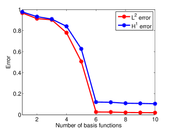
Figure 12: Numerical results with different numbers of basis functions, $H=1/16$, $n_{\text{ov}}=3$, relaxed case.

$10^{2}$ $10^{4}$ $10^{6}$ 3 2.59e-02 1.10e-01 5.64e-01 4 2.21e-02 2.66e-02 1.28e-01

Table 9: Comparison of ($e_{H^{1}}$) various number of oversampling layers and different contrast values for test model 2, relaxed case, $H=1/16,N_{b}=8$.

Dof	H	$n_{\text{ov}}$	$e_{L^{2}}$	$e_{H^{1}}$
24576	1/16	3	2.63e-02	1.21e-01
27951	1/16	3	8.61e-05	4.04e-03
31326	1/16	3	1.94e-06	1.02e-03

Table 10: Uniform enrichment error decay history for the test model 2, $H=1/16$, 6 offline basis used.

Dof	H	$n_{\text{ov}}$	$e_{L^{2}}$	$e_{H^{1}}$
24576	1/16	3	2.63e-02	1.21e-01
25521	1/16	3	2.43e-04	2.54e-02
26602	1/16	3	4.51e-05	1.31e-02
27798	1/16	3	3.10e-05	1.02e-02

Table 11: Adaptive enrichment with $\theta=0.1$ error decay history for the test model 2, $H=1/16$, 6 offline basis used.

7 Conclusions

In this paper, we propose Constraint Energy Minimizing GMsFEM for solving linear elasticity problems in high-contrast media. We introduce the construction of offline and online Constraint Energy Minimizing multiscale basis functions. To construct the offline basis, we first construct an auxiliary space, and then solve energy minimizing problems in target coarse block. The online basis is construct via solving a local problem in a oversampling domain with the residual as source. We provided numerical tests on 2D and 3D models to demonstrate the accuracy of our method.

References

- [1] T. Arbogast, G. Pencheva, M.F. Wheeler, and I. Yotov. A multiscale mortar mixed finite element method. Multiscale Modeling & Simulation, 6(1):319–346 (electronic), 2007.
- [2] I. Babuška and J. M. Melenk. The partition of unity method. Int. J. Numer. Meth. Engrg., 40:727–758, 1997.
- [3] H. Chan, E. Chung, and Y. Efendiev. Adaptive mixed GMsFEM for flows in heterogeneous media. Numerical Mathematics: Theory, Methods and Applications, 9(4):497–527, 2016.
- [4] Z. Chen and T.Y. Hou. A mixed multiscale finite element method for elliptic problems with oscillating coefficients. Mathematics of Computation, 72:541–576, 2002.
- [5] E. Chung, Y. Efendiev, and C. Lee. Mixed generalized multiscale finite element methods and applications. Multiscale Modeling & Simulation, 13(1):338–366, 2015.
- [6] E. Chung, Y. Efendiev, and W. Leung. Residual-driven online generalized multiscale finite element methods. Journal of Computational Physics, 302:176–190, 2015.
- [7] E. Chung, Y. Efendiev, and W. Leung. An online generalized multiscale discontinuous galerkin method (gmsdgm) for flows in heterogeneous media. Communications in Computational Physics, 21(2):401–422, 2017.
- [8] Eric T Chung, Yalchin Efendiev, and Shubin Fu. Generalized multiscale finite element method for elasticity equations. GEM-International Journal on Geomathematics, 5(2):225–254, 2014.
- [9] Eric T Chung, Yalchin Efendiev, and Wing Tat Leung. Constraint energy minimizing generalized multiscale finite element method. Computer Methods in Applied Mechanics and Engineering, 339:298–319, 2018.
- [10] Eric T Chung, Yalchin Efendiev, and Wing Tat Leung. Fast online generalized multiscale finite element method using constraint energy minimization. Journal of Computational Physics, 355:450–463, 2018.
- [11] L. J. Durfolsky. Numerical calculation of equivalent grid block permeability tensors of heterogeneous porous media: Water resour res v27, n5, may 1991, p299–708. In International Journal of Rock Mechanics and Mining Sciences & Geomechanics Abstracts, volume 28, page A350. Pergamon, 1991.
- [12] Y. Efendiev, J. Galvis, and X.H. Wu. Multiscale finite element methods for high-contrast problems using local spectral basis functions. Journal of Computational Physics, 230:937–955, 2011.
- [13] Y. Efendiev and T. Hou. Multiscale finite element methods: theory and applications, volume 4. Springer Science & Business Media, 2009.
- [14] Yalchin Efendiev, Juan Galvis, and Thomas Y Hou. Generalized multiscale finite element methods (GMsFEM). Journal of Computational Physics, 251:116–135, 2013.
- [15] Kai Gao, Eric T Chung, Richard L Gibson Jr, Shubin Fu, and Yalchin Efendiev. A numerical homogenization method for heterogeneous, anisotropic elastic media based on multiscale theory. Geophysics, 80(4):D385–D401, 2015.
- [16] T. Hou and X.H. Wu. A multiscale finite element method for elliptic problems in composite materials and porous media. Journal of Computational Physics, 134:169–189, 1997.
- [17] P. Jenny, S.H. Lee, and H. Tchelepi. Multi-scale finite volume method for elliptic problems in subsurface flow simulation. Journal of Computational Physics, 187:47–67, 2003.
- [18] M.F. Wheeler, G. Xue, and I. Yotov. A multiscale mortar multipoint flux mixed finite element method. ESAIM Math. Model. Numer. Anal., 46(4):759–796, 2012.
- [19] X. Wu, Y. Efendiev, and T. Y. Hou. Analysis of upscaling absolute permeability. Discrete and Continuous Dynamical Systems Series B, 2(2):185–204, 2002.
- [20] Y. Yang, E.Chung, and Fu. S. An enriched multiscale mortar space for high contrast flow problems. Communications in Computational Physics, 2017.
- [21] Yanfang Yang, Eric T Chung, and Shubin Fu. Residual driven online mortar mixed finite element methods and applications. Journal of Computational and Applied Mathematics, 340:318–333, 2018.