Information flow in finite flocks

Abstract

We simulate the canonical Vicsek model and estimate the flow of information as a function of noise (the variability in the extent to which each animal aligns with its neighbours). We show that the global transfer entropy for finite flocks not only fails to peak near the phase transition, as demonstrated for the canonical 2D Ising model, but remains constant from the transition to very low noise values. This provides a foundation for future study regarding information flow in more complex models and real-world flocking data.

1 Introduction

Recent experimental studies of animal flocks, fish [17, 36], birds such as pigeons [34], starlings [18], midges [4] and sheep [23] have dramatically increased our understanding of flocking dynamics. A central theoretical issue is how the communication range between flock members leads to global coordination of the flock, leading to proposals [32, 4] that the flock exists at some critical point—the point at which flocks transition between order and disorder—providing the ideal scenario for collective reaction to external stimuli, with enough order to form collective behaviour without overwhelming inertia. This carries concomitant implications for information flow.

We measure information flow among members of these flocks, using transfer entropy [37], in particular Global Transfer Entropy (GTE, eq. 5), shown to peak on the disordered side of the phase transition in the 2D Ising spin model [9], where mutual information (MI) and pairwise transfer entropy (TE) peak at the transition.

Real world flocks are active matter—systems far from equilibrium, which do not conserve momentum or other dynamical quantities [22]. We analyse the long-term limit GTE of the minimalist Standard Vicsek Model (SVM) [40] of collective motion [38, 41] using a novel closed-form dimensional reduction, obtained by exploiting an approximate isometry in the SVM. This approach has demonstrated anomalous behaviour in MI [11], diverging as noise tends to zero and failing to peak at the transition.

This study reveals two unexpected information-theoretic differences from the Ising model [9] at long observation times: absence of a peak in GTE on the disordered side of the phase transition; and a slowly changing value below the transition. For shorter observation times, unlike the Ising model, the GTE peaks at, rather than above, the phase transition.

While the final closed-form expression for GTE (eq. 9) requires an isometry approximation, two technical innovations (eqs. 6 and 7) were needed to reduce computational requirements (without isometry): replacing the multi-dimensional vector of interacting particles with a consensus vector; and exploiting the independence of the noise, leading to the surprising result (eq. 7) that calculation of global information flow requires no measurement of neighbouring particles.

This new behaviour may inform future studies on real-world flocks or other more sophisticated models, noting that for the SVM maximum information flow occurs not just near the phase transition, but throughout the entire ordered regime as well.

2 The Standard Vicsek Model

The SVM comprises a set of $N$ point particles (labelled $i=1,\ldots,N$) moving on a plane of linear extent $L$ with periodic boundary conditions (see [1] for full details). Each particle moves with constant speed $v$, and interacts only with neighbouring particles within a fixed radius $r$. Positions $\vec{x}_{i}(t)$ and headings $\theta_{i}(t)$ are updated synchronously at discrete time intervals $\Delta t=1$ according to

$$\vec{x}_{i}(t+\Delta t) =\vec{x}_{i}(t)+\vec{v}_{i}(t)\Delta t$$ (1)

$$\theta_{i}(t+\Delta t) =\varphi_{i}(t)+\omega_{i}(t)$$ (2)

respectively, $\varphi_{i}(t)$ is the average heading of all particles within the interaction radius, $r_{i}$, of particle $i$ (including particle $i$ itself), and $\omega_{i}(t)$ is white noise uniform on the interval $[-\eta/2,\eta/2]$ with intensity $\eta\in(0,2\pi]$. The average heading [40], which constructs the consensus vector, is $\varphi_{i}(t)=\arctan[\langle\sin(\theta(t))\rangle_{i,r}/\langle\cos(\theta(t))\rangle_{i,r}]$, where $\langle z\rangle_{i,r}\equiv\frac{1}{N}\sum_{j}^{N}z_{j}\delta_{r}(i,j)$ and $\delta_{r}(i,j)$ is $1$ if neighbour $j$ is within the interaction radius, $r$, of particle $i$, and $0$ otherwise; note that $\delta_{r}(i,i)=1$, so that $z_{i}$ is always included in the average. The velocity vector $\vec{v}_{i}(t)$ is constructed from the heading $\theta_{i}(t)$ with constant speed $v$. Particle density $\rho=N/L^{2}$ is fixed throughout at $0.25$.

Considering the SVM as a steady-state statistical ensemble of finite size containing $N$ particles with control parameter $\eta$, we use capitals to indicate quantities sampled from the ensemble; in particular, $\Theta_{i}$ denotes an ensemble sample of the heading of the $i$th particle. The full order parameter for the SVM ensemble is the 2D mean particle velocity vector $\boldsymbol{M}$ with magnitude $M\in[0,1]$ and heading $\Phi\in(0,2\pi]$ [1]. $M=1$ iff all particles are aligned, while in the fully-disordered case ($\eta=2\pi$) we have $M\to 0$ in the large-system limit $N\to\infty$. The ensemble variance

$$\chi=\langle M^{2}\rangle-\langle M\rangle^{2}$$ (3)

defines the susceptibility; a peak in $\chi$ as a function of $\eta$ is taken to locate an (approximate) phase transition [5].

The phase transition in the original SVM was thought to be second order, but this was disputed [25, 19] and it transpired that seemingly minor details affect the nature of the transition: type of noise statistics [20]; forward versus backward updating (especially at high particle velocities) [33]; boundary conditions associated with density bands or spin waves [2]; and the cone of influence on each particle [21, 35]. The consensus for SVM now appears to state that the phase transition is second order for low velocities, and first order for high velocities [3, 7, 8]. Consequently, we utilise the original SVM model (backward updating, angular noise, periodic boundary conditions and low density) over a range of velocities. Observation of the Binder cumulant [15] for these regimes (not shown) indeed shows a sharp minimum—representative of a first order transition—only at high velocity magnitudes ($v=2.00$), consistent with [3].

The finite-size SVM exhibits behaviours [10] akin to “continuously-broken ergodicity” [30]. Over short observation windows the SVM is confined to a comparatively small volume of phase space, thus breaking symmetry and ergodicity. As the window increases, the SVM explores progressively larger volumes of phase space, until ergodicity is restored, albeit requiring very long windows at low noise.

Thus the ensemble statistics are observation time-dependent [10], giving two regimes—short-term and long-term statistics. In the short-term regime, we collate statistics (with no ergodic assumptions) over ranges of observation sizes spanning several orders of magnitude, demonstrating the effect of observation time. In the long-term limit, since ergodicity is unbroken, the time average of the GTE will be equal to the ensemble average, and thus statistics can be measured from ensembles constructed of many independent realisations—each with shorter observation windows—rather than the prohibitively long time spans required for solitary realisations to traverse the entire phase space.

3 Global Transfer Entropy

The information flow between two continuous random processes, from $Y$ to $X$, is given by the TE [37] :

$$\mathcal{T}_{Y\to X}={\mathbf{H}}(X^{\prime}\,|\,X)-{\mathbf{H}}(X^{\prime}\,|\,X,Y)\,,$$ (4)

where $X,Y$ are the process histories, and $X^{\prime}$ is the updated state. We truncate process histories to just the most recent state as in [9]. For a continuous random variable $X$, ${\mathbf{H}}(X)\equiv-\int p_{X}(x)\log p_{X}(x)dx$ denotes differential entropy, which necessitates a continuous estimator [28]. GTE extends TE to measure information flow from the entire system to a single particle, and here is defined as the ensemble statistic

$$\mathcal{T}_{gl}\equiv\mathcal{T}_{\boldsymbol{\Theta}\to\Theta_{I}}={\mathbf{H}}(\Theta^{\prime}_{I}\,|\,\Theta_{I})-{\mathbf{H}}(\Theta^{\prime}_{I}\,|\,\boldsymbol{\Theta})$$ (5)

where $I$ is uniform on the set of particle indices, $\Theta^{\prime}_{i}$ is the updated heading at time $t+1$ of the $i$th particle, $\boldsymbol{\Theta}=(\Theta_{1},\ldots,\Theta_{N})$ is the vector of all $N$ particle headings.

Since the update of a particle’s heading is mediated purely by the consensus heading of its neighbours, the GTE may be reduced to three dimensions, i.e., ${\mathbf{H}}(\Theta^{\prime}_{I}\,|\,\boldsymbol{\Theta})={\mathbf{H}}(\Theta^{\prime}_{I}\,|\,\Phi_{I})$, giving:

$$\mathcal{T}_{gl}\equiv\mathcal{T}_{\Phi_{I}\to\Theta_{I}}={\mathbf{H}}(\Theta^{\prime}_{I}\,|\,\Theta_{I})-{\mathbf{H}}(\Theta^{\prime}_{I}\,|\,\Phi_{I})\,,$$ (6)

thus eliminating dimensionality issues surrounding $\boldsymbol{\Theta}$.

Noting that $\theta^{\prime}_{i}=[\varphi_{i}+\omega_{i}]$ for any particle $i$—where $[\ldots]$ denotes modulo $2\pi$, confining the result to $(-\pi,\pi]$—and that noise $\omega_{i}$ is independent of $\varphi_{i}$ we have just ${\mathbf{H}}(\Theta^{\prime}_{I}\,|\,\Phi_{I})={\mathbf{H}}(\Omega)$ where $\Omega$ is the (ensemble) noise.

Thus all measurement of particle neighbours is eliminated and eq. 6 reduces to the two dimensional:

$$\mathcal{T}^{2D}_{gl}={\mathbf{H}}(\Theta^{\prime}_{I}\,|\,\Theta_{I})-{\mathbf{H}}(\Omega)\,.$$ (7)

Finally, in the long term limit rotational symmetry remains approximately unbroken: that is, for any fixed angle $\alpha$, the joint distribution $(\Theta_{1}+\alpha,\ldots,\Theta_{N}+\alpha)$ is the same as the joint distribution $(\Theta_{1},\ldots,\Theta_{N})$. Under this isotropy approximation (see below), eq. 7 reduces to a one-dimensional form in which only changes in particle heading $\theta^{\prime}_{i}-\theta_{i}$ and noise $\Omega$ appear. Let $p(\theta_{1},\theta_{2})$ be the probability density function (pdf) of $(\Theta^{\prime}_{I},\Theta_{I})$ [1]. Under the assumption of rotational symmetry we have:

$$p(\theta_{1},\theta_{2})=\frac{1}{2\pi}q(\theta_{1}-\theta_{2})\,,$$ (8)

where $q(\theta)$ is the pdf of $\Theta_{I}-\Theta^{\prime}_{I}$. Since the marginal distributions of $\Theta_{I}$ and $\Theta^{\prime}_{I}$ are uniform on the unit circle in the long-term (ergodic) limit, we obtain ${\mathbf{H}}(\Theta^{\prime}_{I}\,|\,\Theta_{I})={\mathbf{H}}([\Theta^{\prime}_{I}-\Theta_{I}])$ which reduces eq. 7 to the closed-form expression

$$\mathcal{T}^{LT}_{gl}={\mathbf{H}}([\Theta^{\prime}_{I}-\Theta_{I}])-{\mathbf{H}}(\Omega)\,,$$ (9)

for the long-term GTE, where $[\cdots]$ denotes the internal angle. Note that at $\eta=2\pi$, ${\mathbf{H}}([\Theta^{\prime}_{I}-\Theta_{I}])={\mathbf{H}}(\Omega)=\log 2\pi$ and thus $\mathcal{T}^{LT}_{gl}$ vanishes at maximum noise, as expected. As noise decreases, the particles align more and more strongly, so that the distributions of both $\Theta^{\prime}_{I}-\Theta_{I}$ and $\Omega$ become increasingly sharply peaked. Since these are both differential entropies, they both diverge to $-\infty$. The exact nature of the divergence is established in simulations discussed below.

The isotropy approximation arises because the SVM on a 2D plane with periodic boundary conditions—i.e. a flat torus—is not in fact strictly isotropic. We tested its validity by repeating the long-term simulations while randomly rotating the SVM frame of reference between each update, thus enforcing isotropy [6]. Negligible error was introduced around the phase transition and at very low noise [1].

4 Results And Discussion

Figure 1 shows the long-term GTE $\mathcal{T}^{LT}_{gl}$ estimated in sample according to eq. 9 for a range of particle velocities. For $v<0.5$ there is no peak in GTE and for $v\geq 0.5$ peaks occur at or below the phase transition—identified as a peak in $\chi$ as per eq. 3—with all GTE values approaching approximately $0.72$ bits as noise tends to zero. As $v$ increases, a shift in the $\chi$ peak to higher noise values occurs.

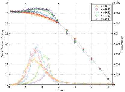
Figure 1: Long-term GTE $\mathcal{T}^{LT}_{gl}$ (dotted) calculated according to eq. 9 for a range of particle velocities for $0<\eta\leq 2\pi$. System size $N=1000$ particles, density $\rho=0.25$ and velocities $v$ as indicated. Simulation: ensembles constructed from $20$ realisations at observation time $T=500$ time steps each, under ergodic assumptions and the isotropy approximation (see text). Error bars at $1$ s.e. (smaller than symbols) were constructed by $10$ repetitions of the experiment. Lines show susceptibility $\chi$ (eq. 3).

For short observation times, by contrast, $\mathcal{T}_{gl}$ and $\mathcal{T}^{2D}_{gl}$ estimated according to eqs. 6 and 7 respectively (and with no isotropy assumption) do peak at the transition, rather than in the disordered regime as in the Ising model [9]; see figs. 2 and 3.

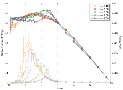
Figure 2: $\mathcal{T}^{2D}_{gl}$ (dark lines) and susceptibility $\chi$ (light lines) estimated for a range of particle velocities (parameters as in fig. 1). $\mathcal{T}^{2D}_{gl}$ was estimated according to eq. 7 over $T=5000$ time steps (that is, with no ergodic assumption) after relaxation to steady state, using a nearest-neighbour estimator (full simulation details in [1]). $\chi$ was estimated over the same realisations. Error bars at $1$ s.e. constructed by $10$ repetitions.

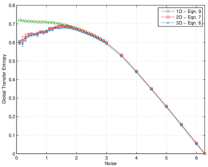
Figure 3: $\mathcal{T}_{gl}$ as measured by the one-dimensional form (eq. 9, circles), the three-dimensional form (eq. 6, crosses) and the two-dimensional form (eq. 7, squares) for $v=0.30$. Error bars at $1$ s.e. constructed by $10$ repetitions.

Figure 3 shows the effect of eliminating the consensus vector measurement in eqs. 6 and 7. The agreement between the two is extremely close, although eq. 7 gives slightly better results for numerical reasons.

Some flattening at low noise occurs, particularly for higher velocities. Here GTE does not converge to the ${\raise 0.73193pt\hbox{$\scriptstyle\mathtt{\sim}$}}0.72$ bits observed in the $\mathcal{T}^{LT}_{gl}$. The shorter the observation window, the nearer we are to ergodicity-breaking as in the Ising Model [9] and thus GTE $\to 0$ as $\eta\to 0$. This is confirmed in fig. 4 which shows $\mathcal{T}^{2D}_{gl}$ for a single fixed velocity at observation window size varying over two orders of magnitude, along with the long-observation time limit $\mathcal{T}^{LT}_{gl}$. As observation time increases, the GTE peak flattens and constant GTE in the ordered regime starts to occur, approaching, as predicted, the long-observation time limit.

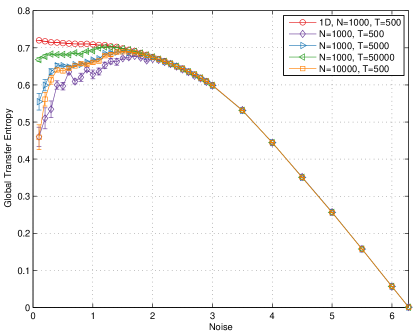
Figure 4: $\mathcal{T}^{2D}_{gl}$ estimates according to eq. 6 at fixed velocity $v=0.30$ for a range of observation times $T$ as indicated, along with the long-term $\mathcal{T}^{LT}_{gl}$ of eq. 9 as per fig. 1. System sizes $N$ as indicated, other simulation details as for previous figures. Note that the blue right triangle line ($N=1000,T=5000$) and orange square line ($N=10000,T=500$) lie on top of each other and represent constant $NT$.

Finally, fig. 5 shows the effect of varying the system size. For $\eta>0.4$, $\mathcal{T}^{2D}_{gl}$ increases—converging to $\mathcal{T}^{LT}_{gl}$—as $N$ increases. Below this however, $\mathcal{T}^{2D}_{gl}$ diverges further as $N$ increases, reflecting the reduced capacity of the system to explore large volumes of the phase space. Near the transition, flocks are in flux, breaking apart and reforming. Given this fluidity, a larger number of particles results in more sub-flocks, which consequently are able to explore the phase space more efficiently, so that the GTE approaches $\mathcal{T}^{LT}_{gl}$. At near-zero noise levels, however, flock stability predominates, with phase space exploration effected mostly by the flock’s random walk-like behaviour [16]. The magnitude of the random walk is inversely proportional to the number of interacting particles; i.e., as the number of interacting particles increases, the mean of the consensus heading at $t+\Delta t$ more closely matches the mean at $t$. Due to the slower random walk, the system explores less of the phase space—more closely approximating ergodicity-breaking—and hence diverges from the long term limit $\mathcal{T}^{LT}_{gl}$.

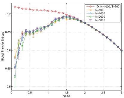
Figure 5: $\mathcal{T}^{2D}_{gl}$ estimates according to eq. 6 at fixed velocity $v=0.30$ for $T=5000$ time steps for varying $N$, along with $\mathcal{T}^{LT}_{gl}$ according to eq. 9 (red circles).

Simulation establishes the nature of the diverging entropies, showing convergence to ${\raise 0.73193pt\hbox{$\scriptstyle\mathtt{\sim}$}}0.72$ bits as $\eta\to 0$. Analysis of how particle headings evolve over time [1] reveals an approximate Gaussian distribution of heading differences—i.e., $\Delta\Theta$—as well as an approximately Gaussian distribution in the heading of the consensus vector—relative to the appropriate particle—as noise tends to zero. From the heading update in eq. 2—with particular note of the definition of $\mathcal{T}^{LT}_{gl}$ in eq. 9—we have:

$$\theta_{i}(t+\Delta t) =\varphi_{i}(t)+\omega_{i}(t)\,,$$ (2 revisited)

$$\theta_{i}(t+\Delta t)-\theta_{i}(t) =\varphi_{i}(t)+\omega_{i}(t)-\theta_{i}(t)\,,$$ (10)

which allows us to decompose $\Delta\Theta$ into two independent distributions, defined by $\varphi_{i}(t)-\theta_{i}(t)$ and $\omega_{i}(t)$. The relative consensus heading, $\varphi_{i}(t)-\theta_{i}(t)$, is approximately Gaussian with support approximately equal to $[-\frac{\eta}{2},\frac{\eta}{2}]$. By definition, noise $\omega_{i}(t)$ is uniform with support $[-\frac{\eta}{2},\frac{\eta}{2}]$. By the Central Limit Theorem [14], summing these two distributions as per the RHS of eq. 10, yields a truncated Gaussian with range $[-\eta,\eta]$ and variance twice that of the noise; i.e., $\sigma^{2}_{\Delta\Theta}=2\sigma^{2}_{\Omega}$. Empirical results match this, with $\sigma^{2}_{\Delta\Theta}=c\sigma^{2}_{\Omega}$ where $c\to 2^{-}$ as $\eta\to 0$.

Thus, closed form entropies for Gaussian and uniform distributions can be substituted into eq. 9:

$$\begin{split}\mathcal{T}^{LT}_{gl}&=\frac{1}{2}\log_{2}2\pi e\sigma_{\Delta\Theta}^{2}-\log_{2}\sqrt{12\sigma_{\Omega}^{2}}\,,\\ &=\frac{1}{2}\log_{2}\frac{2\pi ec\sigma_{\Omega}^{2}}{12\sigma_{\Omega}^{2}}\,,\\ &=\frac{1}{2}\log_{2}\frac{\pi ec}{6}\,,\end{split}$$ (11)

which tends to $0.7546^{-}$ bits as $c\to 2^{-}$, in reasonable agreement with simulation results, given the approximations involved.

Above the phase transition however, the distribution of $\Theta^{\prime}_{I}-\Theta_{I}$ is no longer approximately Gaussian in nature. As $\eta\to 2\pi$, $\Delta\Theta$ becomes increasingly convolved with a uniform distribution before reaching uniformity at $\eta=2\pi$, leading to the decrease seen in $\mathcal{T}_{gl}$ over $\eta_{c}<\eta<2\pi$.

Finite-size scaling analyses [5]—showing good agreement with theory for susceptibility divergence at the phase transition—include the appearance of dense travelling bands of particle at higher velocities (fig. 6) [33]. While this could imply symmetry breaking, fig. 6 reveals that band orientation, as well as $\Phi$, performs a random walk through angle space, thus not truly breaking ergodicity. Notwithstanding, the behaviour of the GTE around the phase transition at higher velocities is indeed different to lower velocities: it exhibits a peak in the long-term limit. The appearance of travelling bands coincides exactly with this noise/velocity regime, indicating that these bands could be a source of information flow.

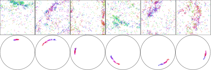
Figure 6: Snapshots from a single simulation demonstrating random walk of heading of high density bands of a flock with $N=1000$ particles at high velocity ($v=2.0$). Snapshots taken at, from left to right, $t=23\times 10^{3},24\times 10^{3},28\times 10^{3},40\times 10^{3},47\times 10^{3},49\times 10^{3}$. Top row shows the state of the flock, while the bottom row shows the two-dimensional order parameter $\boldsymbol{M}$—that is, mean particle velocity—for the previous $1000$ time steps going from blue ($t-1000$) to red ($t$). Distance from the center of the circle corresponds to the order parameter magnitude $M=|\boldsymbol{M}|$. Note that, as witnessed by the first two snapshots, the change in heading can be rapid, with only $1000$ time steps required for the band to precess $\pi/4$ radians. Reprinted from [10].

The flat GTE exhibited in the ordered regime is a result of the approximately Gaussian heading of particles relative to their consensus vectors with variance proportional to noise. Although the continuous nature of the SVM cannot be ruled out at this stage, it seems likely that a “discretised” SVM would display similar behaviour. While it might seem reasonable to have investigated the behaviour of GTE in the continuous equilibrium case for comparison, we note that the obvious contender—the classical XY model—features a BKT phase transition (at least in the 2D case) [27], which would seem to be of an entirely different nature to the transition observed in the 2D SVM model.

It is still a matter of debate whether real-world flocks are poised at criticality. Bialek et al. [13] develop a spin-wave approximation for 3-dimensional flocks of starlings, parametrised from real data. Using this model, along with analysis in [12], Bialek et al. discuss long-range order of the velocity (orientation) and speed fluctuations of the flock. At low noise, there is a spontaneous symmetry breaking of the continuous velocity fluctuations, leaving behind a Goldstone mode [24], wherein there is no energy cost for birds to perform certain changes in flight, which manifests as infinite correlation length [39]. Bialek et al. state, however, that there is no spontaneous symmetry breaking in relation to speed fluctuations, therefore no related Goldstone mode; and hence that long-range order of the flock must be a consequence of criticality.

Melfo [31] instead argues qualitatively that attraction and avoidance rules common in such models do in fact spontaneously break continuous translational invariance, thus giving rise to a Goldstone mode and correlation lengths on the order of the system size. Melfo further states that this should appear in other examples of collective motion—particularly noting the Active-Elastic model of Huepe et al. [26], which achieves scale-free correlation of speed and velocity fluctuations with only attraction and avoidance interaction rules. While we cannot draw any direct conclusions here regarding criticality in real-world flocks—since the SVM utilises constant speed (and thus no speed fluctuations)—our work provides a foundation for further comparative studies of information flow as measured by GTE in alternative models that do feature speed fluctuations.

5 Acknowledgments

We thank Mike Harré, Joe Lizier and Guy Theroulaz for helpful discussions.

The National Computing Infrastructure (NCI) facility provided computing time for the simulations under project e004, with part funding under Australian Research Council Linkage Infrastructure grant LE140100002.

Joshua Brown would like to acknowledge the support of his Ph.D. program and this work from the Australian Government Research Training Program Scholarship.

Lionel Barnett’s research is supported by the Dr. Mortimer and Theresa Sackler Foundation.

References

- [1] See Supplemental Material at [URL].
- [2] M. Aldana, V. Dossetti, Cristián Huepe, V. M. Kenkre, and H. Larralde. Phase transitions in systems of self-propelled agents and related network models. Physical Review Letters, 98:095702–, 2007.
- [3] M Aldana, H Larralde, and B Vázquez. On the emergence of collective order in swarming systems: a recent debate. International Journal of Modern Physics B, 23(18):3661–3685, 2009.
- [4] Alessandro Attanasi, Andrea Cavagna, Lorenzo Del Castello, Irene Giardina, Stefania Melillo, Leonardo Parisi, Oliver Pohl, Bruno Rossaro, Edward Shen, Edmondo Silvestri, et al. Collective behaviour without collective order in wild swarms of midges. PLoS Comput Biol, 10(7):e1003697, 2014.
- [5] Gabriel Baglietto and Ezequiel V. Albano. Finite-size scaling analysis and dynamic study of the critical behavior of a model for the collective displacement of self-driven individuals. Phys. Rev. E, 78:021125, Aug 2008.
- [6] Gabriel Baglietto and Ezequiel V Albano. Nature of the order-disorder transition in the Vicsek model for the collective motion of self-propelled particles. Physical Review E, 80(5):050103, 2009.
- [7] Gabriel Baglietto, Ezequiel V Albano, and Julián Candia. Criticality and the onset of ordering in the standard Vicsek model. Interface Focus, 2(6):708–714, 2012.
- [8] Sonya Bahar. Flocking, swarming, and communicating. In The Essential Tension, pages 127–152. Springer, 2018.
- [9] L.C. Barnett, M. Harré, J.T. Lizier, A. K. Seth, and T. Bossomaier. Information flow in a kinetic Ising model peaks in the disordered phase. Physical Review Letters, 111:177203, 2013.
- [10] Lionel Barnett, Joshua Brown, and Terry Bossomaier. Anomalous behaviour of mutual information in finite flocks. arXiv preprint arXiv:1710.06589, 2017.
- [11] Lionel Barnett, Joshua Brown, and Terry Bossomaier. Anomalous behaviour of mutual information in finite flocks. Europhysics Letters, 120(3):38005, 2018.
- [12] William Bialek, Andrea Cavagna, Irene Giardina, Thierry Mora, Oliver Pohl, Edmondo Silvestri, Massimiliano Viale, and Aleksandra M. Walczak. Social interactions dominate speed control in poising natural flocks near criticality. Proceedings of the National Academy of Sciences, 111(20):7212–7217, 2014.
- [13] William Bialek, Andrea Cavagna, Irene Giardina, Thierry Mora, Edmondo Silvestri, Massimiliano Viale, and Aleksandra M. Walczak. Statistical mechanics for natural flocks of birds. Proceedings of the National Academy of Sciences, 109(13):4786–4791, 2012.
- [14] Patrick Billingsley. Probability and measure, ser. Probability and Mathematical Statistics. New York: Wiley, page 357, 1995.
- [15] Kurt Binder. Theory of first-order phase transitions. Reports on progress in physics, 50(7):783, 1987.
- [16] Joshua M. Brown and Terry Bossomaier. Flock stability in the Vicsek model. In Multiagent System Technologies, pages 89–102. Springer International Publishing, 2017.
- [17] Daniel S. Calovi, Ugo Lopez, Paul Schuhmacher, Hugues Chaté, Clément Sire, and Guy Theraulaz. Collective response to perturbations in a data-driven fish school model. Journal of The Royal Society Interface, 12(104), 2015.
- [18] Andrea Cavagna, Alessio Cimarelli, Irene Giardina, Giorgio Parisi, Raffaele Santagati, Fabio Stefanini, and Massimiliano Viale. Scale-free correlations in starling flocks. Proceedings of the National Academy of Sciences, 107(26):11865–11870, 2010.
- [19] Hugues Chaté, Francesco Ginelli, Guillaume Grégoire, and Franck Raynaud. Collective motion of self-propelled particles interacting without cohesion. Physical Review E, 77:046113–, 2008.
- [20] AA Chepizhko, VL Kulinskii, Yurij Holovatch, Bertrand Berche, Nikolai Bogolyubov, and Reinhard Folk. The kinetic regime of the Vicsek model. In Aip Conference Proceedings, volume 1198, page 25, 2009.
- [21] Mihir Durve and Ahmed Sayeed. First-order phase transition in a model of self-propelled particles with variable angular range of interaction. Physical Review E, 93(5):052115, 2016.
- [22] Étienne Fodor, Cesare Nardini, Michael E Cates, Julien Tailleur, Paolo Visco, and Frédéric van Wijland. How far from equilibrium is active matter? Physical Review Letters, 117(3):038103, 2016.
- [23] Francesco Ginelli, Fernando Peruani, Marie-Helène Pillot, Hugues Chaté, Guy Theraulaz, and Richard Bon. Intermittent collective dynamics emerge from conflicting imperatives in sheep herds. Proceedings of the National Academy of Sciences, 112(41):12729–12734, 2015.
- [24] Jeffrey Goldstone. Field theories with superconductor solutions. Il Nuovo Cimento (1955-1965), 19(1):154–164, 1961.
- [25] Guillaume Grégoire and Hugues Chaté. Onset of collective and cohesive motion. Physical Review Letters, 92(2):025702, 1 2004.
- [26] Cristián Huepe, Eliseo Ferrante, Tom Wenseleers, and Ali Emre Turgut. Scale-free correlations in flocking systems with position-based interactions. Journal of Statistical Physics, 158(3):549–562, 2015.
- [27] John Michael Kosterlitz and David James Thouless. Ordering, metastability and phase transitions in two-dimensional systems. Journal of Physics C: Solid State Physics, 6(7):1181, 1973.
- [28] Alexander Kraskov, Harald Stögbauer, and Peter Grassberger. Estimating mutual information. Physical Review E, 69:066138–066153, 2004.
- [29] David P Landau and K Binder. A guide to monte carlo simulations in statistical physics. 2000.
- [30] J.C. Mauro, P.K. Gupta, and R.J. Loucks. Continuously broken ergodicity. J. Chem. Phys., 126:184511, 2007.
- [31] Alejandra Melfo. A note on spontaneous symmetry breaking in flocks of birds. arXiv preprint arXiv:1702.08067, 2017.
- [32] T. Mora and W. Bialek. Are biological systems poised at criticality? J. Stat. Phys., 144:268–302, 2011.
- [33] Máté Nagy, István Daruka, and Tamás Vicsek. New aspects of the continuous phase transition in the scalar noise model (snm) of collective motion. Physica A: Statistical and Theoretical Physics, 373:445 – 454, 2007.
- [34] Máté Nagy, Gábor Vásárhelyi, Benjamin Pettit, Isabella Roberts-Mariani, Tamás Vicsek, and Dora Biro. Context-dependent hierarchies in pigeons. Proceedings of the National Academy of Sciences, 110(32):13049–13054, 2013.
- [35] Maksym Romensky, Vladimir Lobaskin, and Thomas Ihle. Tricritical points in a Vicsek model of self-propelled particles with bounded confidence. Phys. Rev. E, 90:063315, Dec 2014.
- [36] Sara Brin Rosenthal, Colin R. Twomey, Andrew T. Hartnett, Hai Shan Wu, and Iain D. Couzin. Revealing the hidden networks of interaction in mobile animal groups allows prediction of complex behavioral contagion. Proceedings of the National Academy of Sciences, 112(15):4690–4695, 2015.
- [37] Thomas Schreiber. Measuring information transfer. Physical Review Letters, 85(2):461, 2000.
- [38] John Toner and Yuhai Tu. Flocks, herds, and schools: A quantitative theory of flocking. Physical review E, 58(4):4828, 1998.
- [39] John Toner and Yuhai Tu. Flocks, herds, and schools: A quantitative theory of flocking. Physical review E, 58(4):4828, 1998.
- [40] Tamás Vicsek, András Czirók, Eshel Ben-Jacob, Inon Cohen, and Ofer Shochet. Novel type of phase transition in a system of self-driven particles. Physical Review Letters, 75:1226–1229, 8 1995.
- [41] Tamás Vicsek and Anna Zafeiris. Collective motion. Physics Reports, 517(3–4):71 – 140, 2012.