New Lower Bounds for the Number of
Pseudoline Arrangements

Abstract

Arrangements of lines and pseudolines are fundamental objects in discrete and computational geometry. They also appear in other areas of computer science, such as the study of sorting networks. Let $B_{n}$ be the number of nonisomorphic arrangements of $n$ pseudolines and let $b_{n}=\log_{2}{B_{n}}$. The problem of estimating $B_{n}$ was posed by Knuth in 1992. Knuth conjectured that $b_{n}\leq{n\choose 2}+o(n^{2})$ and also derived the first upper and lower bounds: $b_{n}\leq 0.7924(n^{2}+n)$ and $b_{n}\geq n^{2}/6-O(n)$. The upper bound underwent several improvements, $b_{n}\leq 0.6988\,n^{2}$ (Felsner, 1997), and $b_{n}\leq 0.6571\,n^{2}$ (Felsner and Valtr, 2011), for large $n$. Here we show that $b_{n}\geq cn^{2}-O(n\log{n})$ for some constant $c>0.2083$. In particular, $b_{n}\geq 0.2083\,n^{2}$ for large $n$. This improves the previous best lower bound, $b_{n}\geq 0.1887\,n^{2}$, due to Felsner and Valtr (2011). Our arguments are elementary and geometric in nature. Further, our constructions are likely to spur new developments and improved lower bounds for related problems, such as in topological graph drawings.

Keywords: counting, pseudoline arrangement, recursive construction.

1 Introduction

Arrangements of pseudolines.

A pseudoline in the Euclidean plane is an $x$-monotone curve extending from negative infinity to positive infinity. An arrangement of pseudolines is a family of pseudolines where each pair of pseudolines has a unique point of intersection (called ‘vertex’). An arrangement is simple if no three pseudolines have a common point of intersection, see Fig. 1 (left). Here the term arrangement always means simple arrangement if not specified otherwise.

Figure 1: Left: A simple arrangement ${\mathcal{A}}$. Center: Wiring diagram of ${\mathcal{A}}$. Right: An arrangement ${\mathcal{A}}^{\prime}$ that is not isomorphic to the arrangement ${\mathcal{A}}$ on the left.

There are several representations and encodings of pseudoline arrangements. These representations help one count the number of arrangements. Three classic representations are allowable sequences (introduced by Goodman and Pollack, see, e.g., [10, 11]), wiring diagrams (see for instance [8]), and zonotopal tilings (see for instance [7]). A wiring diagram is an Euclidean arrangement of pseudolines consisting of piece-wise linear ‘wires’, each horizontal except for a short segment where it crosses another wire. Each pair of wires cross exactly once. The wiring diagram in Fig. 1 (center) represents the arrangement ${\mathcal{A}}$. The above representations have been shown to be equivalent; bijective proofs to this effect can be found in [7]. Wiring diagrams are also known as reflection networks, i.e., networks that bring $n$ wires labeled from $1$ to $n$ into their reflection by means of performing switches of adjacent wires; see [14, p. 35]. Lastly, they are also known under the name of primitive sorting networks; see [15, Ch. 5.3.4]. The number of such networks with $n$ wires, i.e., the number of pseudoline arrangements with $n$ pseudolines, is denoted by $A_{n}$. Stanley [20] established the following closed formula for $A_{n}$:

$$A_{n}=\dfrac{\binom{n}{2}!}{\prod_{k=1}^{n-1}(2n-2k-1)^{k}}$$

Two arrangements are isomorphic if they can be mapped onto each other by a homeomorphism of the plane; see Fig. 1. The number of nonisomorphic arrangements of $n$ pseudolines is denoted by $B_{n}$; this is the number of equivalence classes of all arrangements of $n$ pseudolines; see [14, p. 35]. This means that for $A_{n}$, the left to right order of the vertices in the arrangement plays a role while for $B_{n}$ only the order of vertices along each particular pseudoline is important, i.e., the relative position of two vertices from distinct pairs of pseudolines does not matter. We are interested in the growth rate of $B_{n}$; so let $b_{n}=\log_{2}B_{n}$. Knuth [14] conjectured that $b_{n}\leq{n\choose 2}+o(n^{2})$; see also [8, p. 147] and [6, p. 259]. This conjecture is still open.

Upper bounds on the number of pseudoline arrangements.

Felsner [6] used a horizontal encoding of an arrangement in order to estimate $B_{n}$. An arrangement can be represented by a sequence of horizontal cuts. The $i$th cut is the list of the pseudolines crossing the $i$th pseudoline in the order of the crossings. Using this approach, Felsner [6, Thm. 1] obtained the upper bound $b_{n}\leq 0.7213(n^{2}-n)$; he then refined this bound by using replace matrices. A replace matrix is a binary $n\times n$ matrix $M$ with the properties $\sum\nolimits_{j=1}^{n}m_{ij}=n-i$ for all $i$ and $m_{ij}\geq m_{ji}$ for all $i<j$. Using this technique, the author established the upper bound $b_{n}<0.6974\,n^{2}$ [6, Thm. 2].

In his seminal paper on the topic, Knuth [14] took a vertical approach for encoding. Let ${\mathcal{A}}$ be an arrangement of $n$ pseudolines $\{\ell_{1},\ldots,\ell_{n}\}$. By adding pseudoline $\ell_{n+1}$ to ${\mathcal{A}}$, we get ${\mathcal{A}}^{\prime}$, an arrangement of $n+1$ pseudolines. The course of $\ell_{n+1}$ describes a vertical cutpath from top to bottom. The number of cutpaths of ${\mathcal{A}}$ is exactly the number of arrangements ${\mathcal{A}}^{\prime}$ such that ${\mathcal{A}}^{\prime}\setminus\{\ell_{n+1}\}$ is isomorphic to ${\mathcal{A}}$. Let $\gamma_{n}$ denote the maximum number of cutpaths in an arrangement of $n$ pseudolines. Therefore, one has $B_{n+1}\leq\gamma_{n}\cdot B_{n}$; and $B_{3}=2$. Knuth [14] proved that $\gamma_{n}\leq 3^{n}$, concluding that $B_{n}\leq 3^{\binom{n+1}{2}}$ and thus $b_{n}\leq 0.5\,(n^{2}+n)\log_{2}3\leq 0.7924\,(n^{2}+n)$; this computation can be streamlined so that it yields $b_{n}\leq 0.7924\,n^{2}$, see [9]. Knuth also conjectured that $\gamma_{n}\leq n\cdot 2^{n}$, but this was refuted by Ondřej Bílka in 2010 [9]; see also [8, p. 147]. Felsner and Valtr [9] proved a refined result, $\gamma_{n}\leq 4n\cdot 2.48698^{n}$, by a careful analysis. This yields $b_{n}\leq 0.6571\,n^{2}$, which is the current best upper bound.

Lower bounds on the number of pseudoline arrangements.

Knuth [14, p. 37] gave a recursive construction in the setting of reflection networks. The number of nonisomorphic arrangements in his construction, thus also $B_{n}$, obeys the recurrence

$$B_{n}\geq 2^{n^{2}/8-n/4}B_{n/2}.$$

By induction this yields $B_{n}\geq 2^{n^{2}/6-5n/2}$.

Matoušek sketched a simple—still recursive—grid construction in his book [18, Sec. 6.2], see Fig 2. Let $n$ be a multiple of $3$ and $m=\frac{n}{3}$ (assume that $m$ is odd). The $2m$ lines in the two extreme bundles form a regular grid of $m^{2}$ points. The lines in the central bundle are incident to $\frac{3m^{2}+1}{4}$ of these grid points. At each such point, there are $2$ choices; going below it or above it, thus creating at least $\frac{3m^{2}}{4}=\frac{3(n/3)^{2}}{4}=\frac{n^{2}}{12}$ binary choices. Thus $B_{n}$ obeys the recurrence

$$B_{n}\geq 2^{n^{2}/12}B_{n/3}^{3},$$

which by induction yields $B_{n}\geq 2^{n^{2}/8}$.

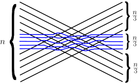
Figure 2: Grid construction for a lower bound on $B_{n}$.

Felsner and Valtr [9] used rhombic tilings of a centrally symmetric hexagon in an elegant recursive construction for a lower bound on $B_{n}$. Consider a set of $i+j+k$ pseudolines partitioned into the following three parts: $\{1,\ldots,i\}$, $\{i+1,\ldots,i+j\}$, $\{i+j+1,\ldots,i+j+k\}$, see Fig. 3. A partial arrangement is called consistent if any two pseudolines from two different parts always cross but any two pseudolines from the same part never cross.

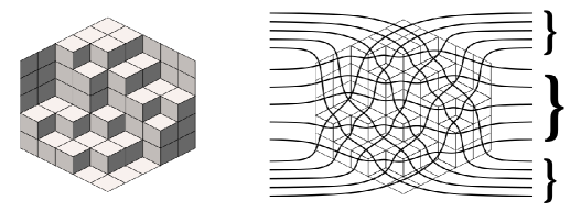
Figure 3: The hexagon $H(5,5,5)$ with one of its rhombic tilings and a consistent partial arrangement corresponding to the tiling. This figure is reproduced from [9].

The zonotopal duals of consistent partial arrangements are rhombic tilings of the centrally symmetric hexagon $H(i,j,k)$ with side lengths $i,j,k$. The enumeration of rhombic tilings of $H(i,j,k)$ was solved by MacMahon [17] (see also [5]), who showed that the number of tilings is

$$P(i,j,k)=\prod\limits_{a=0}^{i-1}\prod\limits_{b=0}^{j-1}\prod\limits_{c=0}^{k-1}\dfrac{a+b+c+2}{a+b+c+1}.$$ (1)

A nontrivial (and quite involved) derivation using integral calculus shows that

$$\ln P(n,n,n)=\left(\frac{9}{2}\ln 3-6\ln 2\right)n^{2}+O(n\log{n})=1.1323\ldots n^{2}+O(n\log{n}).$$

Assuming $n$ to be a multiple of $3$ in the recursion step, the construction yields the lower bound recurrence

$$B_{n}\geq P\bigg{(}\frac{n}{3},\frac{n}{3},\frac{n}{3}\bigg{)}B_{n/3}^{3}.$$ (2)

By induction, the analytic solution to formula (1) together with the recurrence (2) yield the lower bound $B_{n}\geq 2^{cn^{2}-O(n\log^{2}{n})}$, where $c=\frac{3}{4}\ln 3-\ln 2=0.1887\ldots$ In particular, $b_{n}\geq 0.1887\,n^{2}$ for large $n$; this is the previous best lower bound.

Table 1 shows the exact values of $A_{n}$ and $B_{n}$, and their growth rate (up to four digits after the decimal point) with respect to $n$, for small values of $n$. The values of $B_{n}$ for $n=1$ to $9$ are from [14, p. 35] and the values of $B_{10}$, $B_{11}$, and $B_{12}$ are from [6], [21], and [19], respectively; the values of $B_{13}$, $B_{14}$, and $B_{15}$ have been added recently, see [13, 19]. Observe that $A_{n}$ grows much faster than $B_{n}$.

$n$	$A_{n}$	$\dfrac{\log_{2}A_{n}}{n^{2}}$	$B_{n}$	$\dfrac{\log_{2}B_{n}}{n^{2}}$
$1$	$1$	$0$	$1$	$0$
$2$	$1$	$0$	$1$	$0$
$3$	$2$	$0.1111$	$2$	$0.1111$
$4$	$16$	$0.25$	$8$	$0.1875$
$5$	$768$	$0.3833$	$62$	$0.2381$
$6$	$292,864$	$0.5044$	$908$	$0.2729$
$7$	$1,100,742,656$	$0.6129$	$24,698$	$0.2977$
$8$	$48,608,795,688,960$	$0.7104$	$1,232,944$	$0.3161$
$9$	$29,258,366,996,258,488,320$	$0.7983$	$112,018,190$	$0.3301$
$10$			$18,410,581,880$	$0.3409$
$11$			$5,449,192,389,984$	$0.3496$
$12$			$2,894,710,651,370,536$	$0.3566$
$13$			$2,752,596,959,306,389,652$	$0.3624$
$14$			$4,675,651,520,558,571,537,540$	$0.3672$
$15$			$14,163,808,995,580,022,218,786,390$	$0.3713$

Table 1: Values of $A_{n}$ and $B_{n}$ for small $n$.

Our results.

Here we extend the method used by Matoušek in his grid construction; observe that it uses lines of $3$ slopes. In Sections 2 (the 2nd part) and 3, we use lines of $6$ and $12$ different slopes in hexagonal type constructions; yielding lower bounds $b_{n}\geq 0.1981\,n^{2}$ and $b_{n}\geq 0.2083\,n^{2}$ for large $n$, respectively. In Sections A and B of the Appendix, we use lines of $8$ and $12$ different slopes in rectangular type constructions; yielding the lower bounds $b_{n}\geq 0.1999\,n^{2}$ and $b_{n}\geq 0.2053\,n^{2}$ for large $n$, respectively. While the construction in Section 3 gives a better bound, the one in Section 2 is easier to analyze. Results in Section 2, A and B are to appear in [3]. For each of the two styles, rectangular and hexagonal, the constructions are presented in increasing order of complexity. Our main result is summarized in the following.

Theorem 1.

Let $B_{n}$ be the number of nonisomorphic arrangements of $n$ pseudolines. Then $B_{n}\geq 2^{cn^{2}-O(n\log{n})}$, for some constant $c>0.2083$. In particular, $B_{n}\geq 2^{0.2083\,n^{2}}$ for large $n$.

Outline of the proof.

We construct a line arrangement using lines of $k$ different slopes (for a small $k$). The final construction will be obtained by a small clockwise rotation, so that there are no vertical lines. Let $m=\lfloor n/k\rfloor$ or $m=\lfloor n/k\rfloor-1$ (whichever is odd). Each bundle consists of $m$ equidistant lines in the corresponding parallel strip; remaining lines are discarded, or not used in the counting. An $i$-wise crossing is an intersection point of exactly $i$ lines. Let $\lambda_{i}(m)$ denote the number of $i$-wise crossings in the arrangement where each bundle consists of $m$ lines. Our goal is to estimate $\lambda_{i}(m)$ for each $i$. Then we can locally replace the lines around each $i$-wise crossing with any of the $B_{i}$ nonisomorphic pseudoline arrangements; and further apply recursively this construction to each of the $k$ bundles of parallel lines exiting this junction. This yields a simple pseudoline arrangement for each possible replacement choice. Consequently, the number of nonisomorphic pseudoline arrangements in this construction, say, $T(n)$, satisfies the recurrence:

$$T(n)\geq F(n)\left[T\left(\frac{n}{k}\right)\right]^{k},$$ (3)

where $F(n)$ is a multiplicative factor counting the number of choices in this junction:

$$F(n)\geq\prod_{i=3}^{k}B_{i}^{\lambda_{i}(n)}.$$ (4)

Related work.

In a comprehensive recent paper, Kynčl [16] obtained estimates on the number of isomorphism classes of simple topological graphs that realize various graphs. The author remarks that it is probably hard to obtain tight estimates on this quantity, “given that even for pseudoline arrangements, the best known lower and upper bounds on their number differ significantly”. While our improvements aren’t spectacular, it seems however likely that some of the techniques we used here can be employed to obtain sharper lower bounds for topological graph drawings too.

Notations and formulas used.

For two similar figures $F,F^{\prime}$, let $\rho(F,F^{\prime})$ denote their similarity ratio. For a planar region $R$, let ${\rm area}(R)$ denote its area. By slightly abusing notation, let ${\rm area}(i,j,k)$ denote the area of the triangle made by three lines $\ell_{i}$, $\ell_{j}$ and $\ell_{k}$. Assume that the equations of the three lines are $\alpha_{s}x+\beta_{s}y+\gamma_{s}=0$, for $s=1,2,3$, respectively. Then

$${\rm area}(i,j,k) =\frac{A^{2}}{2|C_{1}C_{2}C_{3}|},\text{ where }$$

$$A =\begin{vmatrix}\alpha_{1}&\beta_{1}&\gamma_{1}\\ \alpha_{2}&\beta_{2}&\gamma_{2}\\ \alpha_{3}&\beta_{3}&\gamma_{3}\end{vmatrix},$$

$$C_{1} =(\alpha_{2}\beta_{3}-\beta_{2}\alpha_{3}),$$

$$C_{2} =-(\alpha_{1}\beta_{3}-\beta_{1}\alpha_{3}),$$

$$C_{3} =(\alpha_{1}\beta_{2}-\beta_{1}\alpha_{2}).$$

Let $P(i,j,g,h)$ denote the parallelogram made by the pairs of parallel lines $\ell_{i}\parallel\ell_{j}$ and $\ell_{g}\parallel\ell_{h}$.

2 Preliminary constructions

Warm-up: a rectangular construction with $4$ slopes.

We start with a simple rectangular construction with $4$ bundles of parallel lines whose slopes are $0,\infty,\pm 1$; see Fig. 4. Let $U=[0,1]^{2}$ be the unit square we work with. The axes of all parallel strips are all incident to the center of $U$.

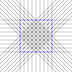
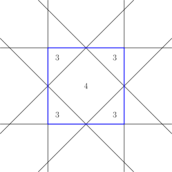
Figure 4: Construction with $4$ slopes; here $m=9$. The unit square $U=[0,1]^{2}$ is shown in blue.

For $i=3,4$, let $a_{i}$ denote the area of the region covered by exactly $i$ of the $4$ strips. It is easy to see that $a_{3}=a_{4}=1/2$, and obviously $a_{3}+a_{4}={\rm area}(U)=1$. Observe that $\lambda_{i}(m)$ is proportional to $a_{i}$, for $i=3,4$; taking the boundary effect into account, we have

$$\lambda_{3}(m)=a_{3}\,m^{2}-O(m)=\frac{m^{2}}{2}-O(m),\text{ and \ \ }\lambda_{4}(m)=a_{4}\,m^{2}-O(m)=\frac{m^{2}}{2}-O(m).$$

Since $m=n/4$, $\lambda_{i}$ can be also viewed as a function of $n$. Therefore $\lambda_{3}(n)=\lambda_{4}(n)=n^{2}/32-O(n)$, and so the multiplicative factor in Eq. (3) is bounded from below as follows:

$$F(n)\geq\prod_{i=3}^{4}B_{i}^{\lambda_{i}(n)}\geq 2^{n^{2}/32-O(n)}\cdot 8^{n^{2}/32-O(n)}=2^{n^{2}/8-O(n)}.$$

By induction on $n$, the resulting lower bound is $T(n)\geq 2^{n^{2}/6-O(n\log{n})}$; this matches the constant $1/6$ in Knuth’s lower bound described in Section 1.

Hexagonal construction with $6$ slopes.

We next describe and analyze a hexagonal construction with lines of $6$ slopes. Consider $6$ bundles of parallel lines whose slopes are $0,\infty,\pm 1/\sqrt{3},\pm\sqrt{3}$. Let $H$ be a regular hexagon whose side has unit length. Three parallel strips are bounded by the pairs of lines supporting opposite sides of $H$, while the other three parallel strips are bounded by the pairs of lines supporting opposite short diagonals of $H$. The axes of all six parallel strips are incident to the center of the circle created by the vertices of $H$; see Fig. 5 (left). This construction yields the lower bound $b_{n}\geq 0.1981\,n^{2}$ for large $n$.

Assume a coordinate system where the lower left corner of $H$ is at the origin, and the lower side of $H$ lies along the $x$-axis. Let ${\mathcal{L}}={\mathcal{L}}_{1}\cup\ldots\cup{\mathcal{L}}_{6}$ be the partition of ${\mathcal{L}}$ into six bundles of parallel lines. The $m$ lines in ${\mathcal{L}}_{i}$ are contained in the parallel strip bounded by the two lines $\ell_{2i-1}$ and $\ell_{2i}$, for $i=1,\ldots,6$. The equation of line $\ell_{i}$ is $\alpha_{i}x+\beta_{i}y+\gamma_{i}=0$, with $\alpha_{i},\beta_{i},\gamma_{i}$, for $i=1,\ldots,12$, given in Fig 5 (right).

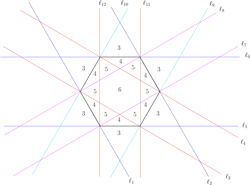
$i$	$\alpha_{i}$	$\beta_{i}$	$\gamma_{i}$
$1$	$\sqrt{3}$	$1$	$0$
$2$	$\sqrt{3}$	$1$	$-2\sqrt{3}$
$3$	$1$	$\sqrt{3}$	$-1$
$4$	$1$	$\sqrt{3}$	$-3$
$5$	$0$	$1$	$0$
$6$	$0$	$1$	$-\sqrt{3}$
$7$	$-1$	$\sqrt{3}$	$0$
$8$	$-1$	$\sqrt{3}$	$-2$
$9$	$-\sqrt{3}$	$1$	$\sqrt{3}$
$10$	$-\sqrt{3}$	$1$	$-\sqrt{3}$
$11$	$-1$	$0$	$1$
$12$	$-1$	$0$	$0$

Figure 5: Left: The six parallel strips and corresponding covering multiplicities. These numbers only show incidences at the $3$-wise crossings made by primary lines. Right: Coefficients of the lines $\ell_{i}$ for $i=1,\ldots,12$.

We refer to lines in ${\mathcal{L}}_{1}\cup{\mathcal{L}}_{3}\cup{\mathcal{L}}_{5}$ as the primary lines, and to lines in ${\mathcal{L}}_{2}\cup{\mathcal{L}}_{4}\cup{\mathcal{L}}_{6}$ as secondary lines. Note that

• the distance between consecutive lines in any of the bundles of primary lines is $\frac{\sqrt{3}}{m}\left(1-O\left(\frac{1}{m}\right)\right)$;

• the distance between consecutive lines in any of the bundles of secondary lines is $\frac{1}{m}\left(1-O\left(\frac{1}{m}\right)\right)$.

Let $\sigma_{0}=\sigma_{0}(m)$ and $\delta_{0}=\delta_{0}(m)$ denote the basic parallelogram and triangle respectively, determined by the consecutive lines in ${\mathcal{L}}_{1}\cup{\mathcal{L}}_{3}\cup{\mathcal{L}}_{5}$; the side length of $\sigma_{0}$ and $\delta_{0}$ is $\frac{2}{m}\left(1-O\left(\frac{1}{m}\right)\right)$. Let $H^{\prime}$ be the smaller regular hexagon bounded by the short diagonals of $H$; the similarity ratio $\rho(H^{\prime},H)$ is equal to $\frac{1}{\sqrt{3}}$. Recall that (i) the area of an equilateral triangle of side $s$ is $\frac{s^{2}\sqrt{3}}{4}$; and (ii) the area of a regular hexagon of side $s$ is $\frac{s^{2}3\sqrt{3}}{2}$; as such, we have

$${\rm area}(H) =\frac{3\sqrt{3}}{2},$$

$${\rm area}(H^{\prime}) =\frac{{\rm area}(H)}{3}=\frac{\sqrt{3}}{2},$$

$${\rm area}(\delta_{0}) =\frac{4}{m^{2}}\frac{\sqrt{3}}{4}\left(1-O\left(\frac{1}{m}\right)\right)=\frac{\sqrt{3}}{m^{2}}\left(1-O\left(\frac{1}{m}\right)\right),$$

$${\rm area}(\sigma_{0}) =2\cdot{\rm area}(\delta_{0})=\frac{2\sqrt{3}}{m^{2}}\left(1-O\left(\frac{1}{m}\right)\right).$$

For $i=3,4,5,6$, let $a_{i}$ denote the area of the (not necessarily connected) region covered by exactly $i$ of the $6$ strips. The following observations are in order: (i) the six isosceles triangles based on the sides of $H$ inside $H$ have unit base and height $\frac{1}{2\sqrt{3}}$; (ii) the six smaller equilateral triangles incident to the vertices of $H$ have side-length $\frac{1}{\sqrt{3}}$. These observations yield

$$a_{3}={\rm area}(H)=\frac{3\sqrt{3}}{2},$$

$$a_{4}=6\cdot{\rm area}(3,5,7)=6\cdot\frac{1}{4\sqrt{3}}=\frac{\sqrt{3}}{2},$$

$$a_{5}=6\cdot{\rm area}(3,7,11)=6\cdot\frac{1}{3}\frac{\sqrt{3}}{4}=\frac{\sqrt{3}}{2},$$

$$a_{6}={\rm area}(H^{\prime})=\frac{\sqrt{3}}{2}.$$

Observe that $a_{4}+a_{5}+a_{6}={\rm area}(H)$. Recall that $\lambda_{i}(m)$ denote the number $i$-wise crossings where each bundle consists of $m$ lines. Note that $\lambda_{i}(m)$ is proportional to $a_{i}$, for $i=4,5,6$. Indeed, $\lambda_{i}(m)$ is equal to the number of $3$-wise crossings of lines in ${\mathcal{L}}_{1}\cup{\mathcal{L}}_{3}\cup{\mathcal{L}}_{5}$ that lie in a region covered by $i$ parallel strips, which is roughly equal to the ratio $\frac{a_{i}}{{\rm area}(\sigma_{0})}$, for $i=4,5,6$. More precisely, taking also the boundary effect of the relevant regions into account, we obtain

$$\lambda_{4}(m)=\frac{a_{4}}{{\rm area}(\sigma_{0})}-O(m)=\frac{\sqrt{3}}{2}\frac{m^{2}}{2\sqrt{3}}-O(m)=\frac{m^{2}}{4}-O(m),$$

$$\lambda_{5}(m)=\frac{a_{5}}{{\rm area}(\sigma_{0})}-O(m)=\frac{m^{2}}{4}-O(m),$$

$$\lambda_{6}(m)=\frac{a_{6}}{{\rm area}(\sigma_{0})}-O(m)=\frac{m^{2}}{4}-O(m).$$

For estimating $\lambda_{3}(m)$, the situation is little bit different, namely, in addition to considering $3$-wise crossings of the primary lines, we also observe $3$-wise crossings of the secondary lines at the centers of the small equilateral triangles contained in $H^{\prime}$. See Fig. 6. It follows that

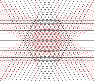
Figure 6: Triple incidences of secondary lines (drawn in red).

$$\lambda_{3}(m)=\frac{a_{3}}{{\rm area}(\sigma_{0})}+\frac{{\rm area}(H^{\prime})}{{\rm area}(\delta_{0})}-O(m)=\frac{3m^{2}}{4}+\frac{m^{2}}{2}-O(m)=\frac{5m^{2}}{4}-O(m).$$

The values of $\lambda_{i}(m)$, for $i=3,4,5,6$, are summarized in Table 2; for convenience the linear terms are omitted. Since $m=n/6$, $\lambda_{i}$ can be also viewed as a function of $n$.

$i$	$3$	$4$	$5$	$6$
$\lambda_{i}(m)$	$\frac{5m^{2}}{4}$	$\frac{m^{2}}{4}$	$\frac{m^{2}}{4}$	$\frac{m^{2}}{4}$
$\lambda_{i}(n)$	$\frac{5n^{2}}{4\cdot 36}$	$\frac{n^{2}}{4\cdot 36}$	$\frac{n^{2}}{4\cdot 36}$	$\frac{n^{2}}{4\cdot 36}$

Table 2: The asymptotic values of $\lambda_{i}(m)$ and $\lambda_{i}(n)$ for $i=3,4,5,6$.

The multiplicative factor in Eq. (3) is bounded from below as follows:

$$F(n)\geq\prod_{i=3}^{6}B_{i}^{\lambda_{i}(n)}\geq 2^{5n^{2}/144}\cdot 8^{n^{2}/144}\cdot 62^{n^{2}/144}\cdot 908^{n^{2}/144}\cdot 2^{-O(n)}.$$

We prove by induction on $n$ that $T(n)\geq 2^{cn^{2}-O(n\log{n})}$ for a suitable constant $c>0$. It suffices to choose $c$ (using the values of $B_{i}$ for $i=3,4,5,6$ in Table 1) so that

$$\frac{8+\log{62}+\log{908}}{144}\geq\frac{5c}{6}.$$

The above inequality holds if we set $c=\dfrac{\log(256\cdot 62\cdot 908)}{120}>0.1981$, and the lower bound follows.

3 Hexagonal construction with $12$ slopes

We next describe and analyze a hexagonal construction with lines of $12$ slopes, which provides our main result in Theorem 1. Consider $12$ bundles of parallel lines whose slopes are $0,\infty,\pm\sqrt{3}/5$, $\pm 1/\sqrt{3},\pm\sqrt{3}/2,\pm\sqrt{3},\pm 3\sqrt{3}$. Let $H$ be a regular hexagon whose side has unit length. The axes of all parallel strips are incident to the center of the circle created by the vertices of $H$; see Figs. 7 and 8. This construction yields the lower bound $b_{n}\geq 0.2083\,n^{2}$ for large $n$.

$i$	$\alpha_{i}$	$\beta_{i}$	$\gamma_{i}$
$1$	$3\sqrt{3}$	$1$	$-\sqrt{3}$
$2$	$3\sqrt{3}$	$1$	$-3\sqrt{3}$
$3$	$\sqrt{3}$	$1$	$0$
$4$	$\sqrt{3}$	$1$	$-2\sqrt{3}$
$5$	$\sqrt{3}$	$2$	$-\sqrt{3}$
$6$	$\sqrt{3}$	$2$	$-2\sqrt{3}$
$7$	$1$	$\sqrt{3}$	$-1$
$8$	$1$	$\sqrt{3}$	$-3$

$i$	$\alpha_{i}$	$\beta_{i}$	$\gamma_{i}$
$9$	$\sqrt{3}$	$5$	$-2\sqrt{3}$
$10$	$\sqrt{3}$	$5$	$-4\sqrt{3}$
$11$	$0$	$1$	$0$
$12$	$0$	$1$	$-\sqrt{3}$
$13$	$-\sqrt{3}$	$5$	$-\sqrt{3}$
$14$	$-\sqrt{3}$	$5$	$-3\sqrt{3}$
$15$	$-1$	$\sqrt{3}$	$0$
$16$	$-1$	$\sqrt{3}$	$-2$

$i$	$\alpha_{i}$	$\beta_{i}$	$\gamma_{i}$
$17$	$-\sqrt{3}$	$2$	$0$
$18$	$-\sqrt{3}$	$2$	$-\sqrt{3}$
$19$	$-\sqrt{3}$	$1$	$\sqrt{3}$
$20$	$-\sqrt{3}$	$1$	$-\sqrt{3}$
$21$	$-3\sqrt{3}$	$1$	$2\sqrt{3}$
$22$	$-3\sqrt{3}$	$1$	$0$
$23$	$-1$	$0$	$1$
$24$	$-1$	$0$	$0$

Table 3: Coefficients of the $24$ lines.

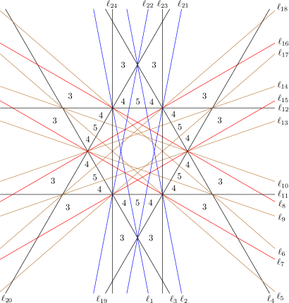
Figure 7: Construction with $12$ slopes. The twelve parallel strips and the corresponding covering multiplicities. These numbers only reflect incidences at the grid vertices made by the primary lines. The numbers inside $H$ are shown in Fig. 8

Assume a coordinate system where the lower left corner of $H$ is at the origin, and the lower side of $H$ lies along the $x$-axis. Let ${\mathcal{L}}={\mathcal{L}}_{1}\cup\ldots\cup{\mathcal{L}}_{12}$ be the partition of ${\mathcal{L}}$ into twelve bundles of parallel lines. The $m$ lines in ${\mathcal{L}}_{i}$ are contained in the parallel strip $\Gamma_{i}$ bounded by the two lines $\ell_{2i-1}$ and $\ell_{2i}$, for $i=1,\ldots,24$. The equation of line $\ell_{i}$ is $\alpha_{i}x+\beta_{i}y+\gamma_{i}=0$, with $\alpha_{i},\beta_{i},\gamma_{i}$, for $i=1,\ldots,24$, given in Table 3.

$\Gamma_{2}$, $\Gamma_{6}$ and $\Gamma_{10}$ are bounded by the pairs of lines supporting opposite sides of $H$, while $\Gamma_{4}$, $\Gamma_{8}$ and $\Gamma_{12}$ are bounded by the pairs of lines supporting opposite short diagonals of $H$. Therefore $H=\Gamma_{2}\cap\Gamma_{6}\cap\Gamma_{10}$. We refer to lines in ${\mathcal{L}}_{2}\cup{\mathcal{L}}_{6}\cup{\mathcal{L}}_{10}$ as the primary lines, to lines in ${\mathcal{L}}_{4}\cup{\mathcal{L}}_{8}\cup{\mathcal{L}}_{12}$ as the secondary lines, and to the rest of the lines as the tertiary lines. Note that

• the distance between consecutive lines in any of the bundles of primary lines is $\frac{\sqrt{3}}{m}\left(1-O\left(\frac{1}{m}\right)\right)$;

• the distance between consecutive lines in any of the bundles of secondary lines is $\frac{1}{m}\left(1-O\left(\frac{1}{m}\right)\right)$;

• the distance between consecutive lines in any of the bundles of tertiary lines is $\sqrt{\frac{3}{7}}\frac{1}{m}\left(1-O\left(\frac{1}{m}\right)\right)$.

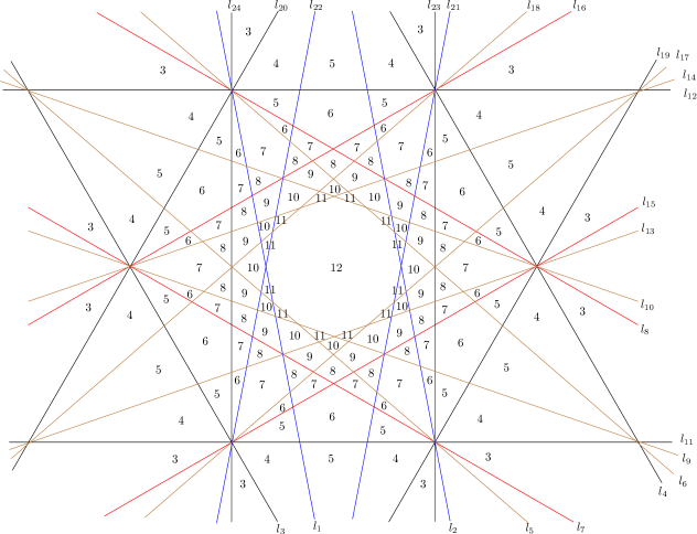
Figure 8: Construction with $12$ slopes. The twelve parallel strips and the corresponding covering multiplicities. These numbers only reflect incidences at the grid vertices made by the primary lines.

We refer to the intersection points of the primary lines as grid vertices. There are two types of grid vertices: the grid vertices in $H$ are intersection of $3$ primary lines and the ones outside $H$ are intersection of $2$ primary lines.

Let $\sigma_{0}=\sigma_{0}(m)$ and $\delta_{0}=\delta_{0}(m)$ denote the basic parallelogram and triangle respectively, determined by the primary lines (i.e., lines in ${\mathcal{L}}_{2}\cup{\mathcal{L}}_{6}\cup{\mathcal{L}}_{10}$); the side length of $\sigma_{0}(m)$ and $\delta_{0}$ is $\frac{2}{m}\left(1-O\left(\frac{1}{m}\right)\right)$. We refer to these basic parallelograms as grid cells. Recall that (i) the area of an equilateral triangle of side $s$ is $\frac{s^{2}\sqrt{3}}{4}$; and (ii) the area of a regular hexagon of side $s$ is $\frac{s^{2}3\sqrt{3}}{2}$; as such, we have

$${\rm area}(H) =\frac{3\sqrt{3}}{2},$$

$${\rm area}(\delta_{0}) =\frac{4}{m^{2}}\frac{\sqrt{3}}{4}\left(1-O\left(\frac{1}{m}\right)\right)=\frac{\sqrt{3}}{m^{2}}\left(1-O\left(\frac{1}{m}\right)\right),$$

$${\rm area}(\sigma_{0}) =2\cdot{\rm area}(\delta_{0})=\frac{2\sqrt{3}}{m^{2}}\left(1-O\left(\frac{1}{m}\right)\right).$$

For $i=3,\ldots,12$, let $a_{i}$ denote the area of the (not necessarily connected) region covered by exactly $i$ of the $6$ strips. Recall that ${\rm area}(i,j,k)$ denotes the area of the triangle made by $\ell_{i}$, $\ell_{j}$ and $\ell_{k}$.

Observe that $a_{12}$ is the area of the $12$-gon $\bigcap_{i=1}^{12}\Gamma_{i}$. This $12$-gon is not regular, since consecutive vertices lie on two concentric cycles of radii $\frac{1}{3}$ and $\frac{\sqrt{3}}{5}$ centered at $(\frac{1}{2},\frac{\sqrt{3}}{2})$. So $a_{12}$ is the sum of the areas of $12$ congruent triangles; each with one vertex at the center of $H$ and other two as the two consecutive vertices of the $12$-gon. Each of these triangles have area $\frac{\sqrt{3}}{60}$. Therefore,

$$a_{12} =12\cdot\frac{\sqrt{3}}{60}=\frac{\sqrt{3}}{5},$$

$$a_{11} =12\cdot{\rm area}(1,5,9)=12\cdot\frac{1}{140\sqrt{3}}=\frac{\sqrt{3}}{35},$$

$$a_{10} =6\cdot({\rm area}(1,5,13)-{\rm area}(1,5,9))+6\cdot({\rm area}(5,9,22)-{\rm area}(1,5,9))$$

$$=6\cdot\left(\frac{\sqrt{3}}{70}-\frac{1}{140\sqrt{3}}\right)+6\cdot\left(\frac{1}{56\sqrt{3}}-\frac{1}{140\sqrt{3}}\right)=\frac{13\sqrt{3}}{140},$$

$$a_{9} =12\cdot({\rm area}(1,7,22)-{\rm area}(1,9,22))=12\cdot\left(\frac{1}{20\sqrt{3}}-\frac{1}{56\sqrt{3}}\right)=\frac{9\sqrt{3}}{70},$$

$$a_{8} =6\cdot({\rm area}(9,22,24)-{\rm area}(7,22,24))+12\cdot{\rm area}(7,13,22)$$

$$=6\cdot\left(\frac{\sqrt{3}}{40}-\frac{1}{20\sqrt{3}}\right)+12\cdot\frac{\sqrt{3}}{140}=\frac{19\sqrt{3}}{140},$$

$$a_{7} =12\cdot({\rm area}(7,22,24)-{\rm area}(13,22,24))+6\cdot({\rm area}(1,17,22)-{\rm area}(1,13,22))$$

$$=12\cdot\left(\frac{1}{20\sqrt{3}}-\frac{\sqrt{3}}{140}\right)+6\cdot\left(\frac{5}{28\sqrt{3}}-\frac{1}{14\sqrt{3}}\right)=\frac{23\sqrt{3}}{70},$$

$$a_{6} =12\cdot({\rm area}(13,22,24))+6\cdot({\rm area}(7,11,15)-2\cdot{\rm area}(1,11,15))$$

$$=12\cdot\frac{\sqrt{3}}{140}+6\cdot\left(\frac{1}{4\sqrt{3}}-2\cdot\frac{1}{20\sqrt{3}}\right)=\frac{27\sqrt{3}}{70},$$

$$a_{5} =12\cdot({\rm area}(1,11,15))+6\cdot({\rm area}(1,11,21))=12\cdot\frac{1}{20\sqrt{3}}+6\cdot\frac{1}{4\sqrt{3}}=\frac{7\sqrt{3}}{10},$$

$$a_{4} =12\cdot({\rm area}(1,3,11))=12\cdot\frac{1}{4\sqrt{3}}=\sqrt{3},$$

$$a_{3} =12\cdot({\rm area}(4,7,11))=12\cdot\frac{\sqrt{3}}{4}=3\sqrt{3}.$$

Observe that the region whose area is $\sum_{i=5}^{12}a_{i}$ consists of the hexagon $H$ and $6$ triangles outside $H$. Therefore,

$$\sum\nolimits_{i=5}^{12}a_{i}={\rm area}(H)+6\cdot{\rm area}(1,11,21)=\frac{3\sqrt{3}}{2}+6\cdot\frac{1}{4\sqrt{3}}=2\sqrt{3}.$$

Recall that $\lambda_{i}(m)$ denotes the number of $i$-wise crossings where each bundle consists of $m$ lines. Note that $\lambda_{i}(m)$ is proportional to $a_{i}$, for $i=5,6,\ldots,12$. Indeed, $\lambda_{i}(m)$ is equal to the number of grid vertices that lie in a region covered by $i$ parallel strips, which is roughly equal to the ratio $\frac{a_{i}}{{\rm area}(\sigma_{0})}$, for $i=5,6,\ldots,12$. More precisely, taking also the boundary effect of the relevant regions into account, we obtain

$$\lambda_{12}(m) =\frac{a_{12}}{{\rm area}(\sigma_{0})}-O(m)=\frac{\sqrt{3}}{5}\frac{m^{2}}{2\sqrt{3}}-O(m)=\frac{m^{2}}{10}-O(m),$$

$$\lambda_{11}(m) =\frac{a_{11}}{{\rm area}(\sigma_{0})}-O(m)=\frac{m^{2}}{70}-O(m),$$

$$\lambda_{10}(m) =\frac{a_{10}}{{\rm area}(\sigma_{0})}-O(m)=\frac{13m^{2}}{280}-O(m),$$

$$\lambda_{9}(m) =\frac{a_{9}}{{\rm area}(\sigma_{0})}-O(m)=\frac{9m^{2}}{140}-O(m),$$

$$\lambda_{8}(m) =\frac{a_{8}}{{\rm area}(\sigma_{0})}-O(m)=\frac{19m^{2}}{280}-O(m),$$

$$\lambda_{7}(m) =\frac{a_{7}}{{\rm area}(\sigma_{0})}-O(m)=\frac{23m^{2}}{140}-O(m),$$

$$\lambda_{6}(m) =\frac{a_{6}}{{\rm area}(\sigma_{0})}-O(m)=\frac{27m^{2}}{140}-O(m),$$

$$\lambda_{5}(m) =\frac{a_{6}}{{\rm area}(\sigma_{0})}-O(m)=\frac{7m^{2}}{20}-O(m).$$

For $i=3,4$, not all the $i$-wise crossings are at grid vertices. It can be exhaustively verified (by hand) that there are $21$ types of crossings; see Fig. 9. Types $1$ through $3$ are $4$-wise crossings and types $4$ through $21$ are $3$-wise crossings. The bundles intersecting at each of these $21$ types of vertices are listed in Table 4. For $j=1,2,\ldots,21$, let $w_{j}$ denote the weighted area containing all the crossings of type $j$; where the weight is the number of crossings per grid cell. To complete the estimates of $\lambda_{i}(m)$ for $i=3,4$, we calculate $w_{j}$ for all $j$ from the bundles intersecting at type $j$ crossings. The values are listed in Table 5. Observe that for two parallel strips $\Gamma_{i}$ and $\Gamma_{j}$, the area of their intersection is ${\rm area}(\Gamma_{i}\cap\Gamma_{j})={\rm area}(P(2i-1,2i,2j-1,2j))$; recall that $P(2i-1,2i,2j-1,2j)$ denotes the parallelogram made by the two pairs of parallel lines $\ell_{2i-1},\ell_{2i}$ and $\ell_{2j-1},\ell_{2j}$, respectively.

$j$	Bundles intersecting at type $j$ vertices
$1$	${\mathcal{L}}_{6},{\mathcal{L}}_{12},{\mathcal{L}}_{3},{\mathcal{L}}_{9}$
$2$	${\mathcal{L}}_{2},{\mathcal{L}}_{8},{\mathcal{L}}_{11},{\mathcal{L}}_{5}$
$3$	${\mathcal{L}}_{10},{\mathcal{L}}_{4},{\mathcal{L}}_{1},{\mathcal{L}}_{7}$
$4$	${\mathcal{L}}_{2},{\mathcal{L}}_{7},{\mathcal{L}}_{9}$
$5$	${\mathcal{L}}_{6},{\mathcal{L}}_{11},{\mathcal{L}}_{1}$
$6$	${\mathcal{L}}_{10},{\mathcal{L}}_{3},{\mathcal{L}}_{5}$
$7$	${\mathcal{L}}_{12},{\mathcal{L}}_{5},{\mathcal{L}}_{7}$

$j$	Bundles intersecting at type $j$ vertices
$8$	${\mathcal{L}}_{4},{\mathcal{L}}_{11},{\mathcal{L}}_{9}$
$9$	${\mathcal{L}}_{8},{\mathcal{L}}_{1},{\mathcal{L}}_{3}$
$10$	${\mathcal{L}}_{1},{\mathcal{L}}_{5},{\mathcal{L}}_{9}$
$11$	${\mathcal{L}}_{11},{\mathcal{L}}_{3},{\mathcal{L}}_{7}$
$12$	${\mathcal{L}}_{12},{\mathcal{L}}_{3},{\mathcal{L}}_{9}$
$13$	${\mathcal{L}}_{4},{\mathcal{L}}_{1},{\mathcal{L}}_{7}$
$14$	${\mathcal{L}}_{8},{\mathcal{L}}_{11},{\mathcal{L}}_{5}$

$j$	Bundles intersecting at type $j$ vertices
$15$	${\mathcal{L}}_{4},{\mathcal{L}}_{8},{\mathcal{L}}_{12}$
$16$	${\mathcal{L}}_{6},{\mathcal{L}}_{12},{\mathcal{L}}_{3}$
$17$	${\mathcal{L}}_{6},{\mathcal{L}}_{12},{\mathcal{L}}_{9}$
$18$	${\mathcal{L}}_{2},{\mathcal{L}}_{8},{\mathcal{L}}_{11}$
$19$	${\mathcal{L}}_{2},{\mathcal{L}}_{8},{\mathcal{L}}_{5}$
$20$	${\mathcal{L}}_{10},{\mathcal{L}}_{4},{\mathcal{L}}_{1}$
$21$	${\mathcal{L}}_{10},{\mathcal{L}}_{4},{\mathcal{L}}_{7}$

Table 4: Bundles intersecting at type $j$ vertices for $j=1,2,\ldots,21$.

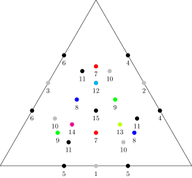
Figure 10: In the $12$-gon in the middle of $H$, all the triangular grid cells contain $3$-crossings and $4$-crossings of all types $1$ through $15$. In other grid cells of the construction only some of these types appear.

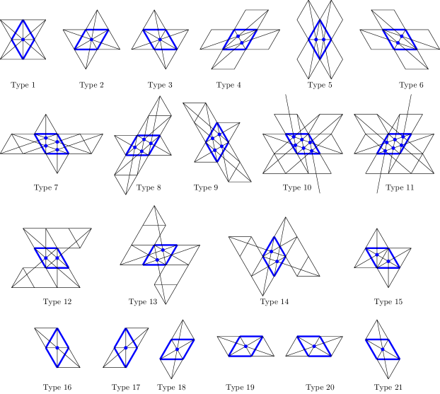
Figure 9: Types of incidences of $3$ and $4$ lines that are not at grid vertices: $4$-wise crossings: types $1$ through $3$; $3$-wise crossings: types $4$ through $21$. To list the coordinates of the crossing points (shown as blue dots), we set the leftmost vertex of the grid cell (shown in blue lines) at $(0,0)$ and the length of the sides of each grid cell as $1$.
For types $1$ through $3$ the crossings are at the center of the parallelogram.
For types $4$ through $6$, the crossings are on the short diagonal at $\frac{1}{3}$rd and $\frac{2}{3}$rd of the short diagonal.
For type $7$, the crossings are at $(\frac{1}{2},\frac{-\sqrt{3}}{10})$, $(\frac{1}{2},\frac{-3\sqrt{3}}{10})$, $(1,\frac{-\sqrt{3}}{5})$, $(1,\frac{-2\sqrt{3}}{5})$.
For type $8$, the crossings are at $(\frac{2}{5},\frac{\sqrt{3}}{5})$, $(\frac{7}{10},\frac{\sqrt{3}}{10})$, $(\frac{4}{5},\frac{2\sqrt{3}}{5})$, $(\frac{11}{10},\frac{3\sqrt{3}}{10})$.
For type $9$, the crossings are at $(\frac{3}{10},\frac{\sqrt{3}}{10})$, $(\frac{2}{5},\frac{-\sqrt{3}}{5})$, $(\frac{3}{5},\frac{\sqrt{3}}{5})$, $(\frac{7}{10},\frac{-\sqrt{3}}{10})$.
For type $10$, the crossings are at $(\frac{5}{14},\frac{-\sqrt{3}}{14})$, $(\frac{5}{7},\frac{-\sqrt{3}}{7})$, $(\frac{15}{14},\frac{-3\sqrt{3}}{14})$, $(\frac{3}{7},\frac{-2\sqrt{3}}{7})$, $(\frac{11}{14},\frac{-5\sqrt{3}}{14})$, $(\frac{8}{7},\frac{-3\sqrt{3}}{7})$.
For type $11$, the crossings are at $(\frac{8}{7},\frac{3\sqrt{3}}{7})$, $(\frac{11}{14},\frac{5\sqrt{3}}{14})$, $(\frac{3}{7},\frac{2\sqrt{3}}{7})$, $(\frac{15}{14},\frac{3\sqrt{3}}{14})$, $(\frac{5}{7},\frac{\sqrt{3}}{7})$, $(\frac{5}{14},\frac{\sqrt{3}}{14})$.
For type $12$, the crossings are at $(\frac{1}{2},\frac{-\sqrt{3}}{4})$ and $(1,\frac{-\sqrt{3}}{4})$.
For type $13$, the crossings are at $(\frac{5}{8},\frac{\sqrt{3}}{8})$ and $(\frac{7}{8},\frac{3\sqrt{3}}{8})$.
For type $14$, the crossings are at $(\frac{3}{8},\frac{\sqrt{3}}{8})$ and $(\frac{5}{8},\frac{-\sqrt{3}}{8})$.
For type $15$, the crossings are on the long diagonal at $\frac{1}{3}$rd and $\frac{2}{3}$rd of the long diagonal.
For types $16$ through $21$ the crossings are at the center of the parallelogram.
The relative positions of all these crossings are shown in Fig. 10.

$\bullet\hskip 5.69054pt$ For $\lambda_{4}(m)$, all the $4$-wise crossings that are not at grid vertices, are at the centers of the grid cells; we have

$$w_{1}={\rm area}(\Gamma_{6}\cap\Gamma_{12}\cap\Gamma_{3}\cap\Gamma_{9})={\rm area}(\Gamma_{3}\cap\Gamma_{9})={\rm area}(P(5,6,17,18))=\frac{\sqrt{3}}{4}.$$

Types $2$ and $3$ are $120^{\circ}$ and $240^{\circ}$ rotations of type $1$, respectively; therefore by symmetry, $w_{1}=w_{2}=w_{3}$.

Consequently, we have

$$\lambda_{4}(n)=\frac{a_{4}+\sum\nolimits_{j=1}^{3}w_{j}}{{\rm area}(\sigma_{0})}-O(m)=\left(\frac{1}{2}+\frac{3}{8}\right)m^{2}-O(m)=\frac{7m^{2}}{8}-O(m).$$

Lastly, we estimate $\lambda_{3}(m)$. Besides $3$-wise crossings at grid vertices in $H$ (whose number is proportional to $a_{3}$), there are $18$ types of $3$-wise crossings i.e., types $4$ through $21$, on the boundary or in the interior of the grid cells in $H$.

• For types $4,5$, and $6$, there are two crossings per grid cell; and

  $$w_{4} =2\cdot{\rm area}(\Gamma_{2}\cap\Gamma_{7}\cap\Gamma_{9})=2\cdot({\rm area}(P(3,4,17,18))-{\rm area}(1,13,17)-{\rm area}(4,14,18))$$

  $$=2\cdot\left(\frac{2}{\sqrt{3}}-\frac{1}{4\sqrt{3}}-\frac{1}{4\sqrt{3}}\right)=\sqrt{3}.$$

  Types $5$ and $6$ are $120^{\circ}$ and $240^{\circ}$ rotations of type $4$, respectively; therefore by symmetry, $w_{4}=w_{5}=w_{6}$.

• For types $7,8$, and $9$, there are four crossings per grid cell; and

  $$w_{7} =4\cdot{\rm area}(\Gamma_{12}\cap\Gamma_{5}\cap\Gamma_{7})=4\cdot({\rm area}(P(9,10,13,14))-{\rm area}(10,13,23)-{\rm area}(9,14,24))$$

  $$=4\cdot\left(\frac{2\sqrt{3}}{5}-\frac{\sqrt{3}}{20}-\frac{\sqrt{3}}{20}\right)=\frac{6\sqrt{3}}{5}.$$

  Types $8$ and $9$ are $120^{\circ}$ and $240^{\circ}$ rotations of type $7$, respectively; therefore by symmetry, $w_{7}=w_{8}=w_{9}$.

• For types $10,11$, there are six crossings per grid cell; and

  $$w_{10} =6\cdot{\rm area}(\Gamma_{1}\cap\Gamma_{5}\cap\Gamma_{9})=6\cdot({\rm area}(P(1,2,17,18))-{\rm area}(1,9,17)-{\rm area}(2,10,18))$$

  $$=6\cdot\left(\frac{2\sqrt{3}}{7}-\frac{\sqrt{3}}{28}-\frac{\sqrt{3}}{28}\right)=\frac{9\sqrt{3}}{7}.$$

  Type $11$ is the reflection in a vertical line of type $10$; therefore by symmetry, $w_{10}=w_{11}$.

• For types $12,13$, and $14$, there are two crossings per grid cell; and

  $$w_{12}=2\cdot{\rm area}(\Gamma_{12}\cap\Gamma_{3}\cap\Gamma_{9})=2\cdot{\rm area}(\Gamma_{3}\cap\Gamma_{9})=2\cdot{\rm area}(P(5,6,17,18))=\frac{\sqrt{3}}{2}.$$

  Types $13$ and $14$ are $120^{\circ}$ and $240^{\circ}$ rotations of type $12$, respectively; therefore by symmetry, $w_{12}=w_{13}=w_{14}$.

• For type $15$, there are two crossings per grid cell; and

  $$w_{15} =2\cdot{\rm area}(\Gamma_{4}\cap\Gamma_{8}\cap\Gamma_{12})=2\cdot({\rm area}(P(15,16,23,24))-{\rm area}(7,15,24)-{\rm area}(8,16,23))$$

  $$=2\cdot\left(\frac{2}{\sqrt{3}}-\frac{1}{4\sqrt{3}}-\frac{1}{4\sqrt{3}}\right)=\sqrt{3}.$$

• For types $16$ through $21$, there is one crossing per grid cell; and

  $$w_{16} ={\rm area}(\Gamma_{6}\cap\Gamma_{12}\cap\Gamma_{3}-\Gamma_{9})={\rm area}(\Gamma_{12}\cap\Gamma_{3})-{\rm area}(\Gamma_{12}\cap\Gamma_{3}\cap\Gamma_{9})$$

  $$={\rm area}(P(5,6,23,24))-{\rm area}(P(5,6,17,18))=\frac{\sqrt{3}}{2}-\frac{\sqrt{3}}{4}=\frac{\sqrt{3}}{4}.$$

  Type $17$ is the reflection in a vertical line of type $16$, types $18$ and $20$ are $120^{\circ}$ and $240^{\circ}$ rotations of type $16$, respectively. Types $19$ and $21$ are $120^{\circ}$ and $240^{\circ}$ rotations of type $17$, respectively. Therefore by symmetry, $w_{16}=w_{17}=w_{18}=w_{19}=w_{20}=w_{21}$.

Consequently, we have

$$\lambda_{3}(n)=\frac{a_{3}+\sum\nolimits_{j=4}^{21}w_{j}}{{\rm area}(\sigma_{0})}-O(m)=\left(\frac{3}{2}+\frac{3}{2}+\frac{9}{5}+\frac{9}{7}+\frac{3}{4}+\frac{1}{2}+\frac{3}{4}\right)m^{2}-O(m)=\frac{283}{35}m^{2}-O(m).$$

$j$	$1$	$2$	$3$	$4$	$5$	$6$	$7$	$8$	$9$	$10$	$11$
$w_{j}$	$\frac{\sqrt{3}}{4}$	$\frac{\sqrt{3}}{4}$	$\frac{\sqrt{3}}{4}$	$\sqrt{3}$	$\sqrt{3}$	$\sqrt{3}$	$\frac{6\sqrt{3}}{5}$	$\frac{6\sqrt{3}}{5}$	$\frac{6\sqrt{3}}{5}$	$\frac{9\sqrt{3}}{7}$	$\frac{9\sqrt{3}}{7}$
$j$	$12$	$13$	$14$	$15$	$16$	$17$	$18$	$19$	$20$	$21$
$w_{j}$	$\frac{\sqrt{3}}{2}$	$\frac{\sqrt{3}}{2}$	$\frac{\sqrt{3}}{2}$	$\sqrt{3}$	$\frac{\sqrt{3}}{4}$	$\frac{\sqrt{3}}{4}$	$\frac{\sqrt{3}}{4}$	$\frac{\sqrt{3}}{4}$	$\frac{\sqrt{3}}{4}$	$\frac{\sqrt{3}}{4}$

Table 5: Values of $w_{j}$ for $j=1,\ldots,21$.

The values of $\lambda_{i}(m)$, for $i=3,\ldots,12$, are summarized in Table 6; for convenience the linear terms are omitted. Since $m=n/12$, $\lambda_{i}$ can be also viewed as a function of $n$.

$i$	$3$	$4$	$5$	$6$	$7$	$8$	$9$	$10$	$11$	$12$
$\lambda_{i}(m)$	$\frac{283m^{2}}{35}$	$\frac{7m^{2}}{8}$	$\frac{7m^{2}}{20}$	$\frac{27m^{2}}{140}$	$\frac{23m^{2}}{140}$	$\frac{19m^{2}}{280}$	$\frac{9m^{2}}{140}$	$\frac{13m^{2}}{280}$	$\frac{m^{2}}{70}$	$\frac{m^{2}}{10}$
$\lambda_{i}(n)$	$\frac{283n^{2}}{35\cdot 144}$	$\frac{7n^{2}}{8\cdot 144}$	$\frac{7n^{2}}{20\cdot 144}$	$\frac{27n^{2}}{140\cdot 144}$	$\frac{23m^{2}}{280\cdot 144}$	$\frac{19n^{2}}{280\cdot 144}$	$\frac{9n^{2}}{140\cdot 144}$	$\frac{13n^{2}}{280\cdot 144}$	$\frac{n^{2}}{70\cdot 144}$	$\frac{n^{2}}{10\cdot 144}$

Table 6: The asymptotic values of $\lambda_{i}(m)$ and $\lambda_{i}(n)$ for $i=3,\ldots,12$.

The multiplicative factor in Eq. (3) is bounded from below as follows:

$$F(n) \geq\prod_{i=3}^{12}B_{i}^{\lambda_{i}(n)}\geq 2^{\frac{283n^{2}}{35\cdot 144}}\cdot 8^{\frac{7n^{2}}{8\cdot 144}}\cdot 62^{\frac{7n^{2}}{20\cdot 144}}\cdot 908^{\frac{27n^{2}}{140\cdot 144}}\cdot 24698^{\frac{23n^{2}}{140\cdot 144}}\cdot 1232944^{\frac{19n^{2}}{280\cdot 144}}$$

$$\cdot 112018190^{\frac{9n^{2}}{140\cdot 144}}\cdot 18410581880^{\frac{13n^{2}}{280\cdot 144}}\cdot 5449192389984^{\frac{n^{2}}{70\cdot 144}}\cdot 2894710651370536^{\frac{n^{2}}{10\cdot 144}}\cdot 2^{-O(n)}.$$

We prove by induction on $n$ that $T(n)\geq 2^{cn^{2}-O(n\log{n})}$ for a suitable constant $c>0$. It suffices to choose $c$ (using the values of $B_{i}$ for $i=3,\ldots,12$ in Table 1) so that

$$\frac{1}{144} \Big{(}\frac{283}{35}+\frac{7}{8}\log{8}+\frac{7}{20}\log{62}+\frac{27}{140}\log{908}+\frac{23}{140}\log{24698}$$

$$+\frac{19}{280}\log{1232944}+\frac{9}{140}\log{112018190}+\frac{13}{280}\log{18410581880}$$

$$+\frac{1}{70}\log{5449192389984}+\frac{1}{10}\log{2894710651370536}\Big{)}\geq\frac{11c}{12}.$$

The above inequality holds if we set

$$\begin{split}c&=\frac{1}{132}\Big{(}\frac{283}{35}+\frac{7}{8}\log{8}+\frac{7}{20}\log{62}+\frac{27}{140}\log{908}+\frac{23}{140}\log{24698}\\ &+\frac{19}{280}\log{1232944}+\frac{9}{140}\log{112018190}+\frac{13}{280}\log{18410581880}\\ &+\frac{1}{70}\log{5449192389984}+\frac{1}{10}\log{2894710651370536}\Big{)}>0.2083,\end{split}$$ (5)

and the lower bound in Theorem 1 follows. ∎

4 Conclusion

We analyzed several recursive constructions derived from arrangements of lines with $3$, $4$, $6$, $8$, and $12$ distinct slopes; in two different styles (rectangular and hexagonal). The hexagonal construction with $12$ slopes yields the lower bound $b_{n}\geq 0.2083\,n^{2}$ for large $n$. We think that increasing the number of slopes will further increase the lower bound, and likely the proof complexity at the same time. The questions of how far can one go and whether there are other more efficient variants remain. We conclude with the following questions.

1. What lower bounds on $B_{n}$ can be deduced from line arrangements with a higher number of slopes? In particular, hexagonal and rectangular constructions with $16$ slopes seem to be the most promising candidates. Note that the value of $B_{16}$ is currently unknown.

2. What lower bounds on $B_{n}$ can be obtained from rhombic tilings of a centrally symmetric octagon? Or from those of a centrally symmetric $k$-gon for some other even $k\geq 10$? No closed formulas for the number of such tilings seem to be available at the time of the present writing. However, suitable estimates could perhaps be deduced from previous results; see, e.g., [1, 2, 4, 12].

Appendix A Rectangular construction with $8$ slopes

We describe and analyze a rectangular construction with lines of $8$ slopes. See Fig. 11. Consider $8$ bundles of parallel lines whose slopes are $0,\infty,\pm 1/2,\pm 1,\pm 2$. The axes of all parallel strips are all incident to the center of $U$. This construction yields the lower bound $b_{n}\geq 0.1999\,n^{2}$ for large $n$.

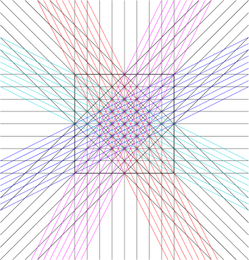
Figure 11: Construction with $8$ slopes.

Let ${\mathcal{L}}={\mathcal{L}}_{1}\cup\ldots\cup{\mathcal{L}}_{8}$ be the partition of ${\mathcal{L}}$ into eight bundles. The $m$ lines in ${\mathcal{L}}_{i}$ are contained in the parallel strip $\Gamma_{i}$ bounded by the two lines $\ell_{2i-1}$ and $\ell_{2i}$, for $i=1,\ldots,8$. The equation of line $\ell_{i}$ is $\alpha_{i}x+\beta_{i}y+\gamma_{i}=0$, with $\alpha_{i},\beta_{i},\gamma_{i}$, for $i=1,\ldots,16$ given in Fig 12 (right). Observe that $U=\Gamma_{4}\cap\Gamma_{8}$.

We refer to lines in ${\mathcal{L}}_{4}\cup{\mathcal{L}}_{8}$ (i.e., axis-aligned lines) as the primary lines, and to rest of the lines as secondary lines. We refer to the intersection points of the primary lines as grid vertices. The slopes of the primary lines are in $\{0,\infty\}$. The slopes of the secondary lines are in $\{\pm 1/2,\pm 1,\pm 2\}$. Note that

• the distance between consecutive lines in ${\mathcal{L}}_{4}$ or ${\mathcal{L}}_{8}$ is $\frac{1}{m}\left(1-O\left(\frac{1}{m}\right)\right)$;

• the distance between consecutive lines in ${\mathcal{L}}_{2}$ or ${\mathcal{L}}_{6}$ is $\frac{1}{m\sqrt{2}}\left(1-O\left(\frac{1}{m}\right)\right)$;

• the distance between consecutive lines in ${\mathcal{L}}_{1}$, ${\mathcal{L}}_{3}$, ${\mathcal{L}}_{5}$ or ${\mathcal{L}}_{7}$ is $\frac{1}{m\sqrt{5}}\left(1-O\left(\frac{1}{m}\right)\right)$.

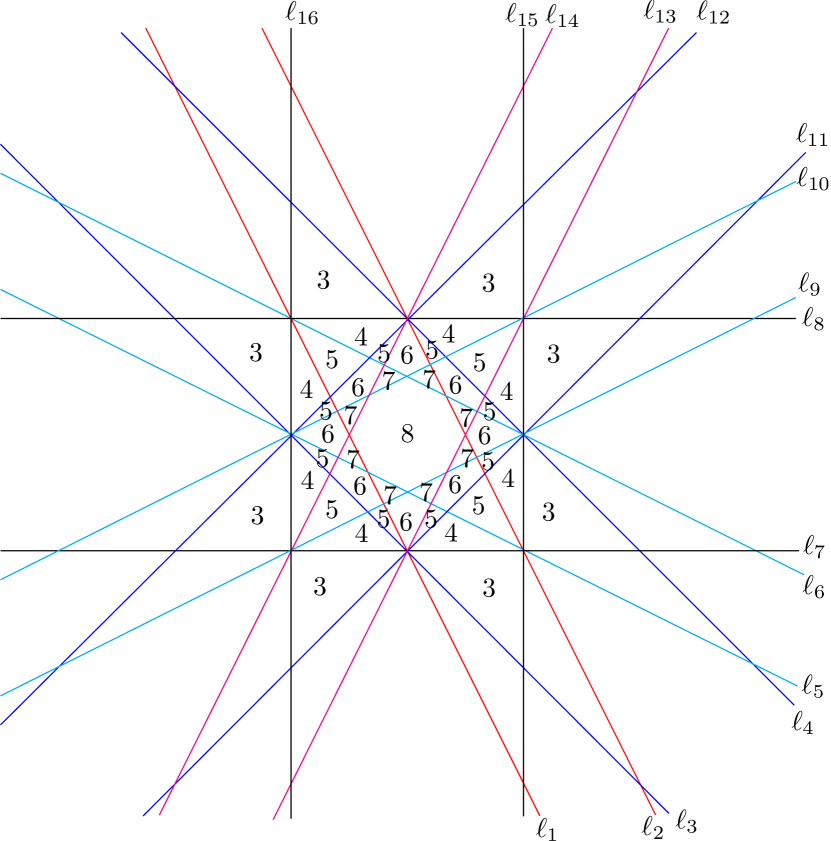
$i$	$\alpha_{i}$	$\beta_{i}$	$\gamma_{i}$
$1$	$2$	$1$	$-1$
$2$	$2$	$1$	$-2$
$3$	$1$	$1$	$-0.5$
$4$	$1$	$1$	$-1.5$
$5$	$1$	$2$	$-1$
$6$	$1$	$2$	$-2$
$7$	$0$	$1$	$0$
$8$	$0$	$1$	$-1$
$9$	$1$	$-2$	$0$
$10$	$1$	$-2$	$1$
$11$	$1$	$-1$	$-0.5$
$12$	$1$	$-1$	$0.5$
$13$	$2$	$-1$	$-1$
$14$	$2$	$-1$	$0$
$15$	$1$	$0$	$-1$
$16$	$1$	$0$	$0$

Figure 12: Left: The eight parallel strips and the corresponding covering multiplicities. These numbers only reflect incidences at the grid vertices made by axis-aligned lines. Right: Coefficients of the lines $\ell_{i}$ for $i=1,2,\ldots,16$.

Let $\sigma_{0}=\sigma_{0}(m)$ denote the basic parallelogram (here, square) determined by consecutive axis-aligned lines (i.e., lines in ${\mathcal{L}}_{4}\cup{\mathcal{L}}_{8}$); the side length of $\sigma_{0}$ is $\frac{1}{m}\left(1-O\left(\frac{1}{m}\right)\right)$. We refer to these basic parallelograms as grid cells. Let $U^{\prime}$ be the smaller square made by $\ell_{5},\ell_{6},\ell_{13},\ell_{14}$, i.e., $U^{\prime}=\Gamma_{3}\cap\Gamma_{7}$; the similarity ratio $\rho(U^{\prime},U)$ is equal to $\frac{1}{\sqrt{5}}$. We have

$${\rm area}(U) =1,$$

$${\rm area}(U^{\prime}) =\frac{{\rm area}(U)}{5}=\frac{1}{5},$$

$${\rm area}(\sigma_{0}) =\frac{1}{m^{2}}\left(1-O\left(\frac{1}{m}\right)\right).$$

For $i=3,4,\ldots,8$, let $a_{i}$ denote the area of the (not necessarily connected) region covered by exactly $i$ of the $8$ strips. Recall that ${\rm area}(i,j,k)$ denotes the area of the triangle made by $\ell_{i}$, $\ell_{j}$ and $\ell_{k}$. We have

$$a_{3} =8\cdot{\rm area}(3,7,15)=1,$$

$$a_{4} =8\cdot{\rm area}(5,7,11)=\frac{1}{3},$$

$$a_{5} =4\left(2\cdot{\rm area}(5,11,13)+{\rm area}(2,5,11)\right)=\frac{7}{30},$$

$$a_{6} =4\left({\rm area}(6,11,13)-2\cdot{\rm area}(2,11,9)-{\rm area}(2,9,13)\right)=\frac{1}{5},$$

$$a_{7} =8\cdot{\rm area}(5,9,13)=\frac{1}{15},$$

$$a_{8} ={\rm area}(U^{\prime})-4\cdot{\rm area}(5,9,13)=\frac{1}{5}-\frac{1}{30}=\frac{1}{6}.$$

Observe that $a_{4}+a_{5}+a_{6}+a_{7}+a_{8}={\rm area}(U)=1$. Recall that $\lambda_{i}(m)$ denote the number of $i$-wise crossings where each bundle consists of $m$ lines. Note that $\lambda_{i}(m)$ is proportional to $a_{i}$, for $i=4,5,6,7,8$. Indeed, $\lambda_{i}(m)$ is equal to the number of grid points that lie in a region covered by $i$ parallel strips, which is roughly equal to the ratio $\frac{a_{i}}{{\rm area}(\sigma_{0})}$, for $i=4,5,6,7,8$. More precisely, taking also the boundary effect of the relevant regions into account, we obtain

$$\lambda_{4}(m) =\frac{a_{4}}{{\rm area}(\sigma_{0})}-O(m)=\frac{m^{2}}{3}-O(m),$$

$$\lambda_{5}(m) =\frac{a_{5}}{{\rm area}(\sigma_{0})}-O(m)=\frac{7m^{2}}{30}-O(m),$$

$$\lambda_{6}(m) =\frac{a_{6}}{{\rm area}(\sigma_{0})}-O(m)=\frac{m^{2}}{5}-O(m),$$

$$\lambda_{7}(m) =\frac{a_{7}}{{\rm area}(\sigma_{0})}-O(m)=\frac{m^{2}}{15}-O(m),$$

$$\lambda_{8}(m) =\frac{a_{8}}{{\rm area}(\sigma_{0})}-O(m)=\frac{m^{2}}{6}-O(m).$$

For estimating $\lambda_{3}(m)$, in addition to considering $3$-wise crossings in the exterior of $U$, we also observe $3$-wise crossings on the boundaries or in the interior of the small grid cells contained in some regions of $U$. Specifically, we distinguish exactly four types of $3$-wise crossings, as illustrated and specified in Fig. 13. For $j=1,2,3,4$, let $w_{j}$ denote the weighted area containing all crossings of type $j$, where the weight is the number of $3$-wise crossings per grid cell. To complete the estimate of $\lambda_{3}(m)$, we calculate $w_{j}$ for all $j$, from the bundles intersecting at crossings of type $j$; listed in Fig. 13 (right).

$j$	Bundles intersecting at vertices of type $j$
$1$	${\mathcal{L}}_{4},{\mathcal{L}}_{1},{\mathcal{L}}_{7}$
$2$	${\mathcal{L}}_{8},{\mathcal{L}}_{3},{\mathcal{L}}_{5}$
$3$	${\mathcal{L}}_{6},{\mathcal{L}}_{1},{\mathcal{L}}_{3}$
$4$	${\mathcal{L}}_{2},{\mathcal{L}}_{5},{\mathcal{L}}_{7}$

Figure 13: Left: Other types of $3$-wise crossings. Right: Intersecting bundles for these crossings.

Recall that for two parallel strips $\Gamma_{i}$ and $\Gamma_{j}$, the area of their intersection is ${\rm area}(\Gamma_{i}\cap\Gamma_{j})={\rm area}(P(2i-1,2i,2j-1,2j))$; where $P(2i-1,2i,2j-1,2j)$ denotes the parallelogram bounded by the two pairs of parallel lines $\ell_{2i-1},\ell_{2i}$ and $\ell_{2j-1},\ell_{2j}$, respectively. For types $1$ and $2$, there is one crossing per grid cell and for types $3$ and $4$, there are two crossings per grid cell. Therefore we have,

• $w_{1}={\rm area}(\Gamma_{4}\cap\Gamma_{1}\cap\Gamma_{7})={\rm area}(\Gamma_{1}\cap\Gamma_{7})={\rm area}(P(1,2,13,14))=1/4$,

• $w_{2}={\rm area}(\Gamma_{8}\cap\Gamma_{3}\cap\Gamma_{5})={\rm area}(\Gamma_{3}\cap\Gamma_{5})={\rm area}(P(5,6,9,10))=1/4$,

• $w_{3}=2\cdot{\rm area}(\Gamma_{1}\cap\Gamma_{3}\cap\Gamma_{6})=2\cdot({\rm area}(P(1,2,5,6))-2\cdot{\rm area}(2,5,11))=2\cdot(1/3-1/12)=1/2$,

• $w_{4}=2\cdot{\rm area}(\Gamma_{2}\cap\Gamma_{5}\cap\Gamma_{7})=1/2$.

It follows that

$$\lambda_{3}(m)=\frac{a_{3}+\sum_{j=1}^{4}w_{j}}{{\rm area}(\sigma_{0})}-O(m)=\left(1+\frac{1}{4}+\frac{1}{4}+\frac{1}{2}+\frac{1}{2}\right)m^{2}-O(m)=\frac{5m^{2}}{2}-O(m).$$

The values of $\lambda_{i}(m)$, for $i=3,4,\ldots,8$, are summarized in Table 7; for convenience the linear terms are omitted. Since $m=n/8$, $\lambda_{i}$ can be also viewed as a function of $n$.

$i$	$3$	$4$	$5$	$6$	$7$	$8$
$\lambda_{i}(m)$	$\frac{5m^{2}}{2}$	$\frac{m^{2}}{3}$	$\frac{7m^{2}}{30}$	$\frac{m^{2}}{5}$	$\frac{m^{2}}{15}$	$\frac{m^{2}}{6}$
$\lambda_{i}(n)$	$\frac{5n^{2}}{2\cdot 64}$	$\frac{n^{2}}{3\cdot 64}$	$\frac{7n^{2}}{30\cdot 64}$	$\frac{n^{2}}{5\cdot 64}$	$\frac{n^{2}}{15\cdot 64}$	$\frac{n^{2}}{6\cdot 64}$

Table 7: The asymptotic values of $\lambda_{i}(m)$ and $\lambda_{i}(n)$ for $i=3,4,\ldots,8$.

The multiplicative factor in Eq. (3) is bounded from below as follows:

$$F(n)\geq\prod_{i=3}^{8}B_{i}^{\lambda_{i}(n)}\geq 2^{\frac{5n^{2}}{2\cdot 64}}\cdot 8^{\frac{n^{2}}{3\cdot 64}}\cdot 62^{\frac{7n^{2}}{30\cdot 64}}\cdot 908^{\frac{n^{2}}{5\cdot 64}}\cdot 24698^{\frac{n^{2}}{15\cdot 64}}\cdot 1232944^{\frac{n^{2}}{6\cdot 64}}\cdot 2^{-O(n)}.$$

We prove by induction on $n$ that $T(n)\geq 2^{cn^{2}-O(n\log{n})}$ for a suitable constant $c>0$. It suffices to choose $c$ (using the values of $B_{i}$ for $i=3,\ldots,8$ in Table 1) so that

$$\frac{1}{64}\left(\frac{5}{2}+\frac{1}{3}\log{8}+\frac{7}{30}\log{62}+\frac{1}{5}\log{908}+\frac{1}{15}\log{24698}+\frac{1}{6}\log{1232944}\right)\geq\frac{7c}{8}.$$

The above inequality holds if we set

$$c=\frac{1}{56}\left(\frac{5}{2}+1+\frac{7}{30}\log{62}+\frac{1}{5}\log{908}+\frac{1}{15}\log{24698}+\frac{1}{6}\log{1232944}\right)>0.1999,$$ (6)

and this yields the lower bound $B_{n}\geq 2^{cn^{2}-O(n\log{n})}$, for some constant $c>0.1999$. In particular, we have $B_{n}\geq 2^{0.1999\,n^{2}}$ for large $n$.

Appendix B Rectangular construction with $12$ slopes

We next describe and analyze a rectangular construction with lines of $12$ slopes. Consider $12$ bundles of parallel lines whose slopes are $0,\infty,\pm 1/3,\pm 1/2,\pm 1,\pm 2,\pm 3$. The axes of all parallel strips are all incident to the center of $U=[0,1]^{2}$. Refer to Fig. 14. This construction yields the lower bound $b_{n}\geq 0.2053\,n^{2}$ for large $n$.

$i$	$\alpha_{i}$	$\beta_{i}$	$\gamma_{i}$
$1$	$3$	$1$	$-1.5$
$2$	$3$	$1$	$-2.5$
$3$	$2$	$1$	$-1$
$4$	$2$	$1$	$-2$
$5$	$1$	$1$	$-0.5$
$6$	$1$	$1$	$-1.5$
$7$	$1$	$2$	$-1$
$8$	$1$	$2$	$-2$

$i$	$\alpha_{i}$	$\beta_{i}$	$\gamma_{i}$
$9$	$1$	$3$	$-1.5$
$10$	$1$	$3$	$-2.5$
$11$	$0$	$1$	$0$
$12$	$0$	$1$	$-1$
$13$	$-1$	$3$	$-0.5$
$14$	$-1$	$3$	$-1.5$
$15$	$-1$	$2$	$0$
$16$	$-1$	$2$	$-1$

$i$	$\alpha_{i}$	$\beta_{i}$	$\gamma_{i}$
$17$	$-1$	$1$	$0.5$
$18$	$-1$	$1$	$-0.5$
$19$	$-2$	$1$	$1$
$20$	$-2$	$1$	$0$
$21$	$-3$	$1$	$1.5$
$22$	$-3$	$1$	$0.5$
$23$	$-1$	$0$	$1$
$24$	$-1$	$0$	$0$

Table 8: Coefficients of the $24$ lines.

Let ${\mathcal{L}}={\mathcal{L}}_{1}\cup\ldots\cup{\mathcal{L}}_{12}$ be the partition of ${\mathcal{L}}$ into twelve bundles. The $m$ lines in ${\mathcal{L}}_{i}$ are contained in the parallel strip $\Gamma_{i}$ bounded by the two lines $\ell_{2i-1}$ and $\ell_{2i}$, for $i=1,\ldots,12$. The equation of line $\ell_{i}$ is $\alpha_{i}x+\beta_{i}y+\gamma_{i}=0$, with $\alpha_{i},\beta_{i},\gamma_{i}$, for $i=1,\ldots,24$ given in Table 8. Observe that $U=\Gamma_{6}\cap\Gamma_{12}$.

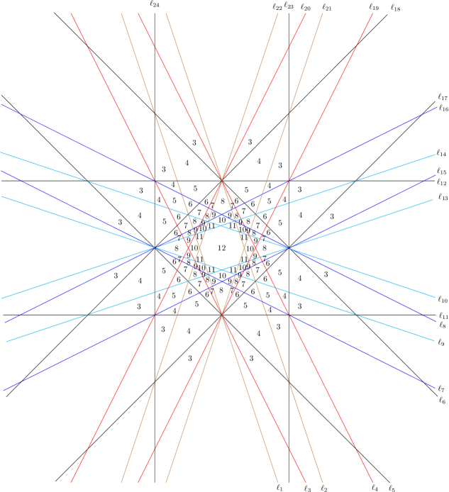
Figure 14: Construction with $12$ slopes. The twelve parallel strips and the corresponding covering multiplicities. These numbers only reflect incidences at the grid vertices made by axis-aligned lines.

We refer to lines in ${\mathcal{L}}_{6}\cup{\mathcal{L}}_{12}$ (i.e., axis-aligned lines) as the primary lines, and to rest of the lines as the secondary lines. We refer to the intersection points of the primary lines as grid vertices. The slopes of the primary lines are in $\{0,\infty\}$, and the slopes of the secondary lines are in $\{\pm 1/3,\pm 1/2,\pm 1,\pm 2,\pm 3\}$.

Note that

• the distance between consecutive lines in ${\mathcal{L}}_{6}$ or ${\mathcal{L}}_{12}$ is $\frac{1}{m}\left(1-O\left(\frac{1}{m}\right)\right)$;

• the distance between consecutive lines in ${\mathcal{L}}_{3}$ or ${\mathcal{L}}_{9}$ is $\frac{1}{m\sqrt{2}}\left(1-O\left(\frac{1}{m}\right)\right)$;

• the distance between consecutive lines in ${\mathcal{L}}_{2}$, ${\mathcal{L}}_{4}$, ${\mathcal{L}}_{8}$, or ${\mathcal{L}}_{10}$ is $\frac{1}{m\sqrt{5}}\left(1-O\left(\frac{1}{m}\right)\right)$;

• the distance between consecutive lines in ${\mathcal{L}}_{1}$, ${\mathcal{L}}_{5}$, ${\mathcal{L}}_{7}$, or ${\mathcal{L}}_{11}$ is $\frac{1}{m\sqrt{10}}\left(1-O\left(\frac{1}{m}\right)\right)$.

Let $\sigma_{0}=\sigma_{0}(m)$ denote the basic parallelogram (here, square) determined by consecutive axis-aligned lines (i.e., lines in ${\mathcal{L}}_{6}\cup{\mathcal{L}}_{12}$); the side length of $\sigma_{0}$ is $\frac{1}{m}\left(1-O\left(\frac{1}{m}\right)\right)$. We refer to these basic parallelograms as grid cells. Let $U_{1}=\Gamma_{1}\cap\Gamma_{7}$, be the square made by $\ell_{1},\ell_{2},\ell_{13},\ell_{14}$, and let $U_{2}=\Gamma_{2}\cap\Gamma_{8}$, be the smaller square made by $\ell_{3},\ell_{4},\ell_{15},\ell_{16}$. Note that $\rho(U_{1},U)=\frac{1}{\sqrt{10}}$ and $\rho(U_{2},U)=\frac{1}{\sqrt{5}}$. We also have

$${\rm area}(U) =1,$$

$${\rm area}(U_{1}) =\frac{{\rm area}(U)}{10}=\frac{1}{10},$$

$${\rm area}(U_{2}) =\frac{{\rm area}(U)}{5}=\frac{1}{5},$$

$${\rm area}(\sigma_{0}) =\frac{1}{m^{2}}\left(1-O\left(\frac{1}{m}\right)\right).$$

For $i=3,\ldots,12$, let $a_{i}$ denote the area of the (not necessarily connected) region covered by exactly $i$ of the $12$ strips. Recall that ${\rm area}(i,j,k)$ denotes the area of the triangle bounded by $\ell_{i}$, $\ell_{j}$ and $\ell_{k}$. We have

$$a_{3} =8\cdot({\rm area}(2,11,13)+{\rm area}(3,5,23))=8\cdot\left(\frac{1}{8}+\frac{1}{24}\right)=\frac{4}{3},$$

$$a_{4} =8\cdot({\rm area}(2,5,11)+{\rm area}(2,7,11))=8\cdot\left(\frac{1}{12}+\frac{1}{120}\right)=\frac{11}{15},$$

$$a_{5} =4\cdot\left({\rm area}(11,17,23)-2\cdot{\rm area}(2,7,11)-2\cdot{\rm area}(2,7,17)\right)=4\left(\frac{1}{8}-\frac{2}{120}-\frac{2}{120}\right)=\frac{11}{30},$$

$$a_{6} =4\cdot\left(2\cdot{\rm area}(7,17,19)+2\cdot{\rm area}(2,7,17)\right)=4\cdot\left(\frac{2}{120}+\frac{2}{120}\right)=\frac{2}{15},$$

$$a_{7} =4\cdot\left(2\cdot{\rm area}(7,19,21)+2\cdot({\rm area}(9,17,19)-{\rm area}(7,17,19))\right)$$

$$=4\cdot\left(\frac{1}{140}+2\cdot\left(\frac{1}{56}-\frac{1}{120}\right)\right)=\frac{11}{105},$$

$$a_{8} =8\cdot\left({\rm area}(9,19,21)-{\rm area}(7,19,21)\right)+4\cdot\left({\rm area}(2,9,15)-{\rm area}(9,15,19)\right)$$

$$+8\cdot{\rm area}(7,21,25)=\frac{13}{105},$$

$$a_{9} =8\cdot({\rm area}(7,15,21)+{\rm area}(9,15,19))=8\cdot\left(\frac{1}{280}+\frac{1}{840}\right)=\frac{4}{105},$$

$$a_{10} =4\cdot\left(({\rm area}(7,13,15)-{\rm area}(9,13,15))+({\rm area}(13,19,21)-{\rm area}(15,19,21))\right)$$

$$=4\cdot\left(\left(\frac{1}{40}-\frac{1}{60}\right)+\left(\frac{1}{80}-\frac{1}{120}\right)\right)=4\cdot\left(\frac{1}{120}+\frac{1}{240}\right)=\frac{1}{20},$$

$$a_{11} =8\cdot{\rm area}(2,13,21)=\frac{8}{240}=\frac{1}{30},$$

$$a_{12} ={\rm area}(U_{1})-4\cdot{\rm area}(9,13,21)=\frac{1}{10}-\frac{4}{240}=\frac{1}{12}.$$

Observe that the region whose area is $\sum_{i=4}^{12}a_{i}$ consists of $U$ and $8$ triangles outside $U$. Therefore,

$$\sum\nolimits_{i=4}^{12}a_{i}={\rm area}(U)+8\cdot{\rm area}(2,5,11)=1+2/3=5/3.$$

Recall that $\lambda_{i}(m)$ denote the number of $i$-wise crossings where each bundle consists of $m$ lines. Note that $\lambda_{i}(m)$ is proportional to $a_{i}$, for $i=7,8,\ldots,12$. Indeed, $\lambda_{i}(m)$ is equal to the number of grid vertices, i.e., intersection points of the axis-parallel lines that lie in a region covered by $i$ parallel strips, which is roughly equal to the ratio $\frac{a_{i}}{{\rm area}(\sigma_{0})}$, for $i=7,8,\ldots,12$. More precisely, taking also the boundary effect of the relevant regions into account, we obtain

$$\lambda_{7}(m) =\frac{a_{7}}{{\rm area}(\sigma_{0})}-O(m)=\frac{11m^{2}}{105}-O(m),$$

$$\lambda_{8}(m) =\frac{a_{8}}{{\rm area}(\sigma_{0})}-O(m)=\frac{13m^{2}}{105}-O(m),$$

$$\lambda_{9}(m) =\frac{a_{9}}{{\rm area}(\sigma_{0})}-O(m)=\frac{4m^{2}}{105}-O(m),$$

$$\lambda_{10}(m) =\frac{a_{10}}{{\rm area}(\sigma_{0})}-O(m)=\frac{m^{2}}{20}-O(m),$$

$$\lambda_{11}(m) =\frac{a_{11}}{{\rm area}(\sigma_{0})}-O(m)=\frac{m^{2}}{30}-O(m),$$

$$\lambda_{12}(m) =\frac{a_{12}}{{\rm area}(\sigma_{0})}-O(m)=\frac{m^{2}}{12}-O(m).$$

For $i=3,4,5,6$, not all the $i$-wise crossings are at grid vertices. It can be exhaustively verified (by hand) that there are $29$ types of such crossings in total; see Fig. 15. The bundles intersecting at each of these $29$ types of vertices are listed in Table 9. For $j=1,2,\ldots,29$, let $w_{j}$ denote the weighted area containing all crossings of type $j$; where the weight is the number of crossings per grid cell. To complete the estimates of $\lambda_{i}(m)$ for $i=3,4,5,6$, we calculate $w_{j}$ for all $j$ from the bundles intersecting at type $j$ crossings. The values are listed in Table 10.

$j$	Bundles intersecting at type $j$ vertices
$1$	${\mathcal{L}}_{2},{\mathcal{L}}_{6},{\mathcal{L}}_{10}$
$2$	${\mathcal{L}}_{4},{\mathcal{L}}_{8},{\mathcal{L}}_{12}$
$3$	${\mathcal{L}}_{2},{\mathcal{L}}_{4},{\mathcal{L}}_{9}$
$4$	${\mathcal{L}}_{3},{\mathcal{L}}_{8},{\mathcal{L}}_{10}$
$5$	${\mathcal{L}}_{3},{\mathcal{L}}_{7},{\mathcal{L}}_{9}$
$6$	${\mathcal{L}}_{3},{\mathcal{L}}_{5},{\mathcal{L}}_{9}$
$7$	${\mathcal{L}}_{3},{\mathcal{L}}_{9},{\mathcal{L}}_{11}$
$8$	${\mathcal{L}}_{1},{\mathcal{L}}_{3},{\mathcal{L}}_{9}$
$9$ & $10$	${\mathcal{L}}_{5},{\mathcal{L}}_{7},{\mathcal{L}}_{12}$

$j$	Bundles intersecting at type $j$ vertices
$11$ & $12$	${\mathcal{L}}_{1},{\mathcal{L}}_{6},{\mathcal{L}}_{11}$
$13$	${\mathcal{L}}_{2},{\mathcal{L}}_{8},{\mathcal{L}}_{11}$
$14$	${\mathcal{L}}_{1},{\mathcal{L}}_{4},{\mathcal{L}}_{10}$
$15$	${\mathcal{L}}_{2},{\mathcal{L}}_{5},{\mathcal{L}}_{8}$
$16$	${\mathcal{L}}_{4},{\mathcal{L}}_{7},{\mathcal{L}}_{10}$
$17$	${\mathcal{L}}_{1},{\mathcal{L}}_{5},{\mathcal{L}}_{9}$
$18$	${\mathcal{L}}_{3},{\mathcal{L}}_{7},{\mathcal{L}}_{11}$
$19$	${\mathcal{L}}_{3},{\mathcal{L}}_{5},{\mathcal{L}}_{7},{\mathcal{L}}_{9}$
$20$	${\mathcal{L}}_{1},{\mathcal{L}}_{3},{\mathcal{L}}_{9},{\mathcal{L}}_{11}$

$j$	Bundles intersecting at type $j$ vertices
$21$	${\mathcal{L}}_{3},{\mathcal{L}}_{7},{\mathcal{L}}_{9},{\mathcal{L}}_{11}$
$22$	${\mathcal{L}}_{1},{\mathcal{L}}_{3},{\mathcal{L}}_{5},{\mathcal{L}}_{9}$
$23$	${\mathcal{L}}_{1},{\mathcal{L}}_{4},{\mathcal{L}}_{7},{\mathcal{L}}_{10}$
$24$	${\mathcal{L}}_{2},{\mathcal{L}}_{5},{\mathcal{L}}_{8},{\mathcal{L}}_{11}$
$25$	${\mathcal{L}}_{1},{\mathcal{L}}_{3},{\mathcal{L}}_{7},{\mathcal{L}}_{9},{\mathcal{L}}_{11}$
$26$	${\mathcal{L}}_{1},{\mathcal{L}}_{3},{\mathcal{L}}_{5},{\mathcal{L}}_{9},{\mathcal{L}}_{11}$
$27$	${\mathcal{L}}_{3},{\mathcal{L}}_{5},{\mathcal{L}}_{7},{\mathcal{L}}_{9},{\mathcal{L}}_{11}$
$28$	${\mathcal{L}}_{1},{\mathcal{L}}_{3},{\mathcal{L}}_{5},{\mathcal{L}}_{7},{\mathcal{L}}_{9}$
$29$	${\mathcal{L}}_{1},{\mathcal{L}}_{3},{\mathcal{L}}_{5},{\mathcal{L}}_{7},{\mathcal{L}}_{9},{\mathcal{L}}_{11}$

Table 9: Bundles intersecting at type $j$ vertices for $j=1,2,\ldots,29$.

For $\lambda_{6}(m)$, all the $6$-wise crossings that are not at grid vertices, are at the centers of grid cells; we have

$$w_{29}={\rm area}(\Gamma_{1}\cap\Gamma_{3}\cap\Gamma_{5}\cap\Gamma_{7}\cap\Gamma_{9}\cap\Gamma_{11})={\rm area}(\Gamma_{1}\cap\Gamma_{5}\cap\Gamma_{7}\cap\Gamma_{11})=a_{12}.$$

It follows that

$$\lambda_{6}(m)=\frac{a_{6}+w_{29}}{{\rm area}(\sigma_{0})}-O(m)=\frac{a_{6}+a_{12}}{{\rm area}(\sigma_{0})}-O(m)=\frac{2m^{2}}{15}+\frac{m^{2}}{12}-O(m)=\frac{13m^{2}}{60}-O(m).$$

Similarly for $\lambda_{5}(m)$, all the $5$-wise crossings that are not at grid vertices, i.e., types $25$ through $28$, are in the interiors of grid cells contained in eight small triangles inside $U$. For example,

$$w_{28}={\rm area}(\Gamma_{1}\cap\Gamma_{3}\cap\Gamma_{5}\cap\Gamma_{7}\cap\Gamma_{9}-\Gamma_{11})={\rm area}(1,14,22)+{\rm area}(2,13,21)=1/120.$$

Observe that sum of the areas of these eight small triangles equals to $a_{11}$. It follows that

$$\lambda_{5}(m)=\frac{a_{5}+\sum\nolimits_{j=25}^{28}w_{j}}{{\rm area}(\sigma_{0})}-O(m)=\frac{a_{5}+a_{11}}{{\rm area}(\sigma_{0})}-O(m)=\frac{11m^{2}}{30}+\frac{m^{2}}{30}-O(m)=\frac{2m^{2}}{5}-O(m).$$

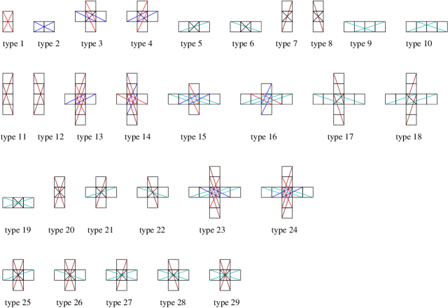
Figure 15: Types of incidences of $3$, $4$, $5$, and $6$ lines that are not at grid vertices: $3$-wise crossings: types $1$ through $18$; $4$-wise crossings: types $19$ through $24$; $5$-wise crossings: types $25$ through $28$; $6$-wise crossings: type $29$.
For some types, the crossings are in the middle of a grid cell. To list the coordinates of crossing points, we rescale the grid cells to the unit square $[0,1]^{2}$.
For types $1$ and $2$, the crossings are at the midpoint of the horizontal and the vertical grid edges respectively. For type $3$, the crossings are at $(1/3,1/3)$ and $(2/3,2/3)$.
For type $4$, the crossings are at $(1/3,2/3)$ and $(2/3,1/3)$.
For types $9$ and $10$, the crossings are on vertical grid edges at height $1/3$ and $2/3$ from the horizontal line below, respectively.
For types $11$ and $12$, the crossings are on horizontal grid edges at distance $1/3$ and $2/3$ from the vertical line on the left, respectively.
For type $13$, the crossings are at $(1/5,3/5)$ and $(3/5,4/5)$ and $(4/5,2/5)$ and $(2/5,1/5)$.
For type $14$, the crossings are at $(1/5,2/5)$ and $(2/5,4/5)$ and $(4/5,3/5)$ and $(3/5,1/5)$.
For type $15$, the crossings are at $(1/5,3/5)$ and $(3/5,4/5)$ and $(4/5,2/5)$ and $(2/5,1/5)$.
For type $16$, the crossings are at $(1/5,2/5)$ and $(2/5,4/5)$ and $(4/5,3/5)$ and $(3/5,1/5)$.
For type $17$, the crossings are at $(1/4,1/4)$ and $(3/4,3/4)$.
For type $18$, the crossings are at $(1/4,3/4)$ and $(3/4,1/4)$.
For type $23$, the crossings are at $(1/5,2/5)$ and $(2/5,4/5)$ and $(4/5,3/5)$ and $(3/5,1/5)$.
For type $24$, the crossings are at $(1/5,3/5)$ and $(3/5,4/5)$ and $(4/5,2/5)$ and $(2/5,1/5)$.
For the other types, the crossings are at $(1/2,1/2)$.

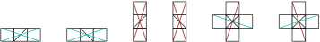
Figure 16: These incidence patterns cannot occur.

To estimate $\lambda_{4}(m)$, note that besides $4$-wise crossings at grid vertices, there are six types of $4$-wise crossings i.e., types $19$ through $24$, in the interiors of grid cells:

• For types $19$ and $20$, there is one crossing per grid cell; and

  $$w_{19} ={\rm area}(\Gamma_{3}\cap\Gamma_{5}\cap\Gamma_{7}\cap\Gamma_{9}-\Gamma_{1}-\Gamma_{11})$$

  $$=({\rm area}(2,10,13)-{\rm area}(2,10,21))+({\rm area}(9,14,22)-{\rm area}(1,14,22))=1/15,$$

  Type $20$ is a $90^{\circ}$ rotation of type $19$; therefore by symmetry, $w_{19}=w_{20}$.

• For types $21$ and $22$, there is one crossing per grid cell; and

  $$w_{21} ={\rm area}(\Gamma_{3}\cap\Gamma_{7}\cap\Gamma_{9}\cap\Gamma_{11}-\Gamma_{1}-\Gamma_{5})$$

  $$=({\rm area}(2,14,21)-{\rm area}(2,10,21))+({\rm area}(1,13,22)-{\rm area}(1,9,22))=1/40.$$

  Type $22$ is the reflection in a vertical line of type $21$; therefore by symmetry, $w_{21}=w_{22}$.

• For types $23$ and $24$, there are four crossings per grid cell; and

  $$w_{23}=4\cdot{\rm area}(\Gamma_{1}\cap\Gamma_{4}\cap\Gamma_{7}\cap\Gamma_{10})=4\cdot{\rm area}(\Gamma_{1}\cap\Gamma_{7})=4\cdot{\rm area}(U_{1})=2/5.$$

  Type $24$ is the reflection in a vertical line of type $23$; therefore by symmetry, $w_{23}=w_{24}$.

Consequently, we have

$$\lambda_{4}(m)=\frac{a_{4}+\sum_{j=19}^{24}w_{j}}{{\rm area}(\sigma_{0})}-O(m)=\Big{(}\frac{11}{15}+\frac{2}{15}+\frac{1}{20}+\frac{4}{5}\Big{)}m^{2}-O(m)=\frac{103m^{2}}{60}-O(m).$$

Lastly, we estimate $\lambda_{3}(m)$. Besides $3$-wise crossings at grid vertices, there are $18$ types of $3$-wise crossings i.e., types $1$ through $18$, in the interior of grid cells:

• For types $1$ and $2$, there is one crossing per grid cell; and

  $$w_{1}={\rm area}(\Gamma_{2}\cap\Gamma_{6}\cap\Gamma_{10})={\rm area}(\Gamma_{2}\cap\Gamma_{10})={\rm area}(P(3,4,19,20))=1/4.$$

  Type $2$ is a $90^{\circ}$ rotation of type $1$; therefore by symmetry, $w_{1}=w_{2}$.

• For types $3$ and $4$, there are two crossings per grid cell; and

  $$w_{3}=2\cdot({\rm area}(\Gamma_{2}\cap\Gamma_{4}\cap\Gamma_{9}))=2\cdot({\rm area}(P(3,4,7,8))-{\rm area}(3,8,18)-{\rm area}(4,7,17))=1/2.$$

  Type $4$ is the reflection in a vertical line of type $3$; therefore by symmetry, $w_{3}=w_{4}$.

• For types $5,6,7,8$, there is one crossing per grid cell; and

  $$w_{5}={\rm area}(\Gamma_{3}\cap\Gamma_{7}\cap\Gamma_{9}-\Gamma_{1}-\Gamma_{5}-\Gamma_{11})={\rm area}(5,9,22)+{\rm area}(6,10,21))=1/20.$$

  Type $6$ is the reflection in a vertical line of type $5$, and types $7$ and $8$ are $90^{\circ}$ rotations of types $6$ and $5$, respectively. Therefore by symmetry, $w_{5}=w_{6}=w_{7}=w_{8}$.

• For types $9,10,11,12$, there is one crossing on the boundary of each grid cell; and

  $$w_{9}={\rm area}(\Gamma_{5}\cap\Gamma_{7}\cap\Gamma_{12})={\rm area}(\Gamma_{5}\cap\Gamma_{7})={\rm area}(P(9,10,13,14))=1/6.$$

  Type $10$ is the reflection in a horizontal line of type $9$, and types $11$ and $12$ are $90^{\circ}$ rotations of types $9$ and $10$, respectively. Therefore by symmetry, $w_{9}=w_{10}=w_{11}=w_{12}$.

• For types $13,14,15,16$, there are four crossings per grid cell; and

  $$w_{13}=4\cdot({\rm area}(\Gamma_{2}\cap\Gamma_{8}\cap\Gamma_{11}-\Gamma_{5}))=4\cdot({\rm area}(3,9,13)+{\rm area}(4,10,16))=1/5.$$

  Type $14$ is the reflection in a vertical line of type $13$, and types $15$ and $16$ are $90^{\circ}$ rotations of types $13$ and $14$, respectively. Therefore by symmetry, $w_{13}=w_{14}=w_{15}=w_{16}$.

• For types $17$ and $18$, there are two crossings per grid cell; and

  $$w_{17}=2\cdot({\rm area}(\Gamma_{1}\cap\Gamma_{5}\cap\Gamma_{9}))=2\cdot({\rm area}(\Gamma_{1}\cap\Gamma_{5}))=2\cdot{\rm area}(P(1,2,9,10))=1/4.$$

  Type $18$ is the reflection in a vertical line of type $17$; therefore by symmetry, $w_{17}=w_{18}$.

Consequently, we have

$$\lambda_{3}(m) =\frac{a_{3}+\sum_{j=1}^{18}w_{j}}{{\rm area}(\sigma_{0})}-O(m)$$

$$=\Big{(}\frac{4}{3}+\frac{1}{2}+1+\frac{1}{10}+\frac{1}{10}+\frac{1}{3}+\frac{1}{3}+\frac{4}{5}+\frac{1}{2}\Big{)}m^{2}-O(m)=5m^{2}-O(m).$$

$j$	$w_{j}$
$1$	$1/4$
$2$	$1/4$
$3$	$1/2$
$4$	$1/2$
$5$	$1/20$
$6$	$1/20$
$7$	$1/20$

$j$	$w_{j}$
$8$	$1/20$
$9$ & $10$	$1/3$
$11$ & $12$	$1/3$
$13$	$1/5$
$14$	$1/5$
$15$	$1/5$
$16$	$1/5$

$j$	$w_{j}$
$17$	$1/4$
$18$	$1/4$
$19$	$1/15$
$20$	$1/15$
$21$	$1/40$
$22$	$1/40$
$23$	$2/5$

$j$	$w_{j}$
$24$	$2/5$
$25$	$1/120$
$26$	$1/120$
$27$	$1/120$
$28$	$1/120$
$29$	$1/12$

Table 10: Values of $w_{j}$ for $j=1,\ldots,29$.

The values of $\lambda_{i}(m)$, for $i=3,4,\ldots,12$, are summarized in Table 11; for convenience the linear terms are omitted. Since $m=n/12$, $\lambda_{i}$ can be also viewed as a function of $n$.

$i$	$3$	$4$	$5$	$6$	$7$	$8$	$9$	$10$	$11$	$12$
$\lambda_{i}(m)$	$5m^{2}$	$\frac{103m^{2}}{60}$	$\frac{2m^{2}}{5}$	$\frac{13m^{2}}{60}$	$\frac{11m^{2}}{105}$	$\frac{13m^{2}}{105}$	$\frac{4m^{2}}{105}$	$\frac{m^{2}}{20}$	$\frac{m^{2}}{30}$	$\frac{m^{2}}{12}$
$\lambda_{i}(n)$	$\frac{5n^{2}}{144}$	$\frac{103n^{2}}{60\cdot 144}$	$\frac{2n^{2}}{5\cdot 144}$	$\frac{13n^{2}}{60\cdot 144}$	$\frac{11n^{2}}{105\cdot 144}$	$\frac{13n^{2}}{105\cdot 144}$	$\frac{4n^{2}}{105\cdot 144}$	$\frac{n^{2}}{20\cdot 144}$	$\frac{n^{2}}{30\cdot 144}$	$\frac{n^{2}}{12\cdot 144}$

Table 11: The asymptotic values of $\lambda_{i}(m)$ and $\lambda_{i}(n)$ for $i=3,4,\ldots,12$.

The multiplicative factor in Eq. (3) is bounded from below as follows:

$$F(n) \geq\prod_{i=3}^{12}B_{i}^{\lambda_{i}(n)}\geq 2^{\frac{5n^{2}}{144}}\cdot 8^{\frac{103n^{2}}{60\cdot 144}}\cdot 62^{\frac{2n^{2}}{5\cdot 144}}\cdot 908^{\frac{13n^{2}}{60\cdot 144}}\cdot 24698^{\frac{11n^{2}}{105\cdot 144}}\cdot 1232944^{\frac{13n^{2}}{105\cdot 144}}$$

$$\cdot 112018190^{\frac{4n^{2}}{105\cdot 144}}\cdot 18410581880^{\frac{n^{2}}{20\cdot 144}}\cdot 5449192389984^{\frac{n^{2}}{30\cdot 144}}\cdot 2894710651370536^{\frac{n^{2}}{12\cdot 144}}\cdot 2^{-O(n)}.$$

We prove by induction on $n$ that $T(n)\geq 2^{cn^{2}-O(n\log{n})}$ for a suitable constant $c>0$. It suffices to choose $c$ (using the values of $B_{i}$ for $i=3,\ldots,12$ in Table 1) so that

$$\frac{1}{144} \Big{(}5+\frac{103}{60}\log{8}+\frac{2}{5}\log{62}+\frac{13}{60}\log{908}+\frac{11}{105}\log{24698}+\frac{13}{105}\log{1232944}+\frac{4}{105}\log{112018190}$$

$$+\frac{1}{20}\log{18410581880}+\frac{1}{30}\log{5449192389984}+\frac{1}{12}\log{2894710651370536}\Big{)}\geq\frac{11c}{12}.$$

The above inequality holds if we set

$$\begin{split}c=\frac{1}{132}\Big{(}5&+\frac{103}{60}\log{8}+\frac{2}{5}\log{62}+\frac{13}{60}\log{908}+\frac{11}{105}\log{24698}\\ &+\frac{13}{105}\log{1232944}+\frac{4}{105}\log{112018190}+\frac{1}{20}\log{18410581880}\\ &+\frac{1}{30}\log{5449192389984}+\frac{1}{12}\log{2894710651370536}\Big{)}>0.2053.\end{split}$$ (7)

References

- [1] N. Destainville, R. Mosseri, and F. Bailly, Fixed-boundary octagonal random tilings: a combinatorial approach, Journal of Statistical Physics 102(1-2) (2001), 147–190.
- [2] N. Destainville, R. Mosseri, and F. Bailly, A formula for the number of tilings of an octagon by rhombi, Theoretical Computer Science 319 (2004), 71–81.
- [3] A. Dumitrescu and R. Mandal, New lower bounds for the number of pseudoline arrangements, Proc. 30th ACM-SIAM Symposium on Discrete Algorithms (SODA 2019), to appear.
- [4] S. Elnitsky, Rhombic tilings of polygons and classes of reduced words in Coxeter groups, Journal of Combinatorial Theory Ser. A 77 (1997), 193–221.
- [5] V. Elser, Solution of the dimer problem on an hexagonal lattice with boundary, Journal of Physics A: Mathematical and General 17:1509 (1984).
- [6] S. Felsner, On the number of arrangements of pseudolines, Discrete & Computational Geometry 18 (1997), 257–267.
- [7] S. Felsner, Geometric Graphs and Arrangements, Advanced Lectures in Mathematics, Vieweg Verlag, 2004.
- [8] S. Felsner and J. E. Goodman, Pseudoline arrangements, in Handbook of Discrete and Computational Geometry (3rd edition), (J. E. Goodman, J. O’Rourke, C. D. Tóth, editors), CRC Press, Boca Raton (2017), pp. 125–157.
- [9] S. Felsner and P. Valtr, Coding and counting arrangements of pseudolines, Discrete & Computational Geometry 46(4) (2011), 405–416.
- [10] J. E. Goodman and R. Pollack, A combinatorial perspective on some problems in geometry, Congressus Numerantium 32 (1981), 383–394.
- [11] J. E. Goodman and R. Pollack, Allowable sequences and order types in discrete and computational geometry, in New Trends in Discrete and Computational Geometry (J. Pach, editor), Algorithms and Combinatorics, Volume 10, Springer, New York, 1993, pp. 103–134.
- [12] M. Hutchinson and M. Widom, Enumeration of octagonal tilings, Theoretical Computer Science 598 (2015), 40–50.
- [13] J. Kawahara, T. Saitoh, R. Yoshinaka, and S. Minato. Counting primitive sorting networks by . Technical Report, Hokkaido University, TCS-TR-A-11-54, 2011. http://www-alg.ist.hokudai.ac.jp/~thomas/TCSTR/tcstr_11_54/tcstr_11_54.pdf
- [14] D. E. Knuth, Axioms and Hulls, Lecture Notes in Computer Science, Vol. 606, Springer, Berlin, 1992.
- [15] D. E. Knuth, The Art of Computer Programming, Vol. 3: Sorting and Searching, 2nd edition, Addison–Wesley, Reading, MA, 1998.
- [16] J. Kynčl, Improved enumeration of simple topological graphs, Discrete & Computational Geometry 50(3) (2013), 727–770.
- [17] P. A. MacMahon, Combinatory Analysis, vol. II, Chelsea, New York, 1960. Reprint of the 1916 edition.
- [18] J. Matoušek, Lectures on Discrete Geometry, Springer, New York, 2002.
- [19] N. Sloane and S. Plouffe, The On-Line Encyclopedia of Integer Sequences, http://oeis.org/A006245 (accessed March 11, 2018).
- [20] R. Stanley, On the number of reduced decompositions of elements of Coxeter groups, European Journal of Combinatorics 5 (1984), 359–372.
- [21] K. Yamanaka, S. Nakano, Y. Matsui, R. Uehara, and K. Nakada, Efficient enumeration of all ladder lotteries and its application, Theoretical Computer Science 411(16-18) (2010), 1714–1722.