A physical approach to modelling large-scale galactic magnetic fields

Abstract

Context. A convenient representation of the structure of the large-scale galactic magnetic field is required for the interpretation of polarization data in the sub-mm and radio ranges, in both the Milky Way and external galaxies.

Aims. We develop a simple and flexible approach to construct parametrised models of the large-scale magnetic field of the Milky Way and other disc galaxies, based on physically justifiable models of magnetic field structure. The resulting models are designed to be optimised against available observational data.

Methods. Representations for the large-scale magnetic fields in the flared disc and spherical halo of a disc galaxy were obtained in the form of series expansions whose coefficients can be calculated from observable or theoretically known galactic properties. The functional basis for the expansions is derived as eigenfunctions of the mean-field dynamo equation or of the vectorial magnetic diffusion equation.

Results. The solutions presented are axially symmetric but the approach can be extended straightforwardly to non-axisymmetric cases. The magnetic fields are solenoidal by construction, can be helical, and are parametrised in terms of observable properties of the host object, such as the rotation curve and the shape of the gaseous disc. The magnetic field in the disc can have a prescribed number of field reversals at any specified radii. Both the disc and halo magnetic fields can separately have either dipolar or quadrupolar symmetry. The model is implemented as a publicly available software package galmag which allows, in particular, the computation of the synchrotron emission and Faraday rotation produced by the model’s magnetic field.

Conclusions. The model can be used in interpretations of observations of magnetic fields in the Milky Way and other spiral galaxies, in particular as a prior in Bayesian analyses. It can also be used for a simple simulation of a time-dependent magnetic field generated by dynamo action.

1 Introduction

Recent increased interest in the large-scale magnetic fields of the Milky Way (MW) and other spiral galaxies is driven by a number of factors. Their role in the dynamics of the interstellar medium (ISM) has been widely appreciated although not completely understood. Their significance for the feedback processes in evolving galaxies has also been recognised and is being actively explored (e.g. Fire2). Furthermore, the separation of the Galactic foreground, including its magnetic field and associated emission, from extragalactic contributions is essential to identify the sources of ultra-high energy cosmic rays (UHECR) (KoOl11; MoRo18) and for cosmological interpretations of sensitive CMB observations (e.g. PlanckXI2018).

Our understanding of the Galactic magnetic field (GMF) is based on observations of Faraday rotation of polarised radio emission, synchrotron emission of energetic electrons, and polarised emission and absorption by dust (e.g. haverkorn2015). Observations of external spiral galaxies have provided rich polarisation data for their discs and haloes (Beck15; Wiegert2015; Mao2015). Interpretation of such data in terms of three-dimensional magnetic field structures requires parametrised models of the magnetic field based on the understanding of their nature and origin. It can be expected that models that rely less on specific theoretical models would have a larger number of free parameters whose physical meaning would be less clear. On the contrary, physically motivated models can be more flexible and lead to physically transparent interpretations of observations.

A range of heuristic models for the structure of the GMF have been proposed (e.g. Sun2008; Jaffe2010; VanEck2011; JF12; JF12a; Ferriere2014; Terral2017). Magnetic fields in most of these models are superpositions of various ad hoc parts whose parameters are selected by fitting to a range of observables. The heuristic nature of the models makes them rather inflexible. Furthermore, their parameters are not necessarily related to the ISM properties (often lacking a transparent physical meaning), and some such models fail to satisfy even such fundamental constraints as $\nabla\cdot\bm{B}=0$ or to allow for the global helical nature of galactic magnetic fields that imprints on its structure and symmetries. The ambiguities, problems and limitations of the current approaches to GMF modelling have been discussed in Planck16 and by the IMAGINE consortium (IMAGINE).

A possible way to overcome heuristics in GMF modelling would be to extract the field structure from physical simulations of galaxy formation and evolution, which include all relevant processes of magnetic field generation and are specific to the MW. Such simulations of generic galaxies have led to important insights into various magnetic structures in spiral galaxies (e.g. Pakmor2017; 2013MNRAS.432..176P) but their resolution remains insufficient to capture galactic dynamo action, as it is controlled by turbulent processes on scales less than 100 pc. Moreover, the simulations would have to be constrained in a way flexible enough to reproduce an ever increasing set of observational data.

Here we propose a simple (that is, flexible, adjustable, analytic) and yet realistic (i.e., based on relevant equations and observations) approach to model the large-scale (mean) magnetic field in the disc and halo of the Milky Way and other spiral galaxies. The model has been implemented as a publicly available software package galmag (GALMAG_zenodo), which can be used in the framework of Bayesian optimisers (e.g. Steininger2018; Steininger2018ASCL)

The text is organised as follows. In Section 2, we lay out the modelling strategy, basic equations and fundamental assumptions. In Section 3, we describe the solutions for magnetic field in the disc and in Section LABEL:sec:SDS, for the halo. In Section LABEL:sec:discuss we discuss possible applications of this model to the interpretation of observations of synchrotron emission and Faraday rotation (Section LABEL:sec:radio) as well some of the ways in which it could be used to model the evolution of galactic magnetic fields (Section LABEL:sec:Bevol); possible extensions to this model are also discussed (Section LABEL:sec:EM), whilst Section LABEL:galmag introduces the publicly available galmag software package that implements the model. Our results are summarised in Section LABEL:sec:final.

2 Basic equations

A physically meaningful model of a galactic magnetic field has to rely on a clear physical picture of its origin and maintenance, as well as on a specific galaxy model. Mean-field dynamo action is the most plausible mechanism of generation and maintenance of large-scale magnetic fields in spiral galaxies (RSS88; Beck1996; BrSu05; Beck15). Therefore, we first explore the nature of magnetic structures compatible with dynamo action. However, magnetic fields observed in galaxies have many features that emerge independently of the dynamo process. To allow for such features, we make our model rather independent of the specific properties of dynamo-generated magnetic fields and use solutions of the dynamo equations just as a convenient functional basis to parametrise a wide class of magnetic structures. Furthermore, we discuss how an even more general type of the governing equations can be used for these purposes.

The dynamo converts kinetic energy of random (turbulent) flows into magnetic energy. The mean helicity of the random flow, that emerges because of the overall rotation and stratification, leads to the generation of magnetic fields at scales much larger than the correlation scale of the random flow (this is described as the $\alpha$-effect). Differential rotation can accelerate the energy conversion by stretching the large-scale magnetic fields in the direction of the flow (the $\omega$-effect). The spatial scale and structure of the magnetic field are controlled by the mean-field transport coefficients, quantifying the averaged induction effects of the random flows, and the large-scale velocity shear rate. The magnetic field structure also depends upon the geometric shape of the dynamo region (e.g. spherical, toroidal or flat). When the magnetic field is weak, so that its effect on the velocity field is negligible, the dynamo leads to an exponential amplification of the large-scale magnetic field. As the Lorentz force becomes stronger, the field growth slows down and the system gradually settles into a (statistically) steady state: the dynamo action saturates.

The mean-field dynamo equation has the form

$$\frac{\partial\bm{B}}{\partial t}=\nabla\times(\alpha\bm{B})+\nabla\times(\bm{V}\times\bm{B})+\beta\nabla^{2}\bm{B}\,,$$ (1)

where $\bm{B}$ is the large-scale magnetic field, $\alpha$ and $\beta$ are the turbulent transport coefficients representing the mean induction effects of the helical interstellar turbulence (the $\alpha$-effect) and turbulent magnetic diffusion, respectively, and $\bm{V}$ is the large-scale velocity field. The latter is dominated by differential rotation but can also include galactic outflows (fountain or wind) and accretion.

Detailed reviews of the galactic dynamo and comprehensive references can be found in RSS88; Beck1996; ShukurovMAND; ShukurovSubramanian2018. We present here a very short overview of the theory with the number of specific references reduced to a minimum.

The mean-field galactic dynamo equation has been solved under various approximations that cover a wide range of galactic environments. Our goal is to present a general class of physically-motivated magnetic field models that can be used to fit observations without the need to delve too deeply into the theory. Thus, we present a parametrised model with the large-scale magnetic field in the form of an expansion over appropriate basis functions, specifically the modes of free decay which solve the diffusion equation in the disc and spherical geometries. The form of the magnetic structures obtained is controlled by the choice of the expansion coefficients. The large-scale magnetic field in the model consists of a superposition of approximate solutions of the kinematic mean-field dynamo equations for a thin disc (Section 3) and a spherical gaseous halo (Section LABEL:sec:SDS). Our use of the dynamo equations is less restrictive than it might seem since their solutions can be used as a functional basis to represent a wide class of complex magnetic configurations, not necessarily produced by dynamo action, in terms of a small number of the expansion coefficients. Unlike representations in terms of the Euler potentials (Ferriere2014), magnetic configurations presented here can be helical. Another advantage of our approach is that all variables and parameters of the model are either directly observable or related to observable quantities.

The approximate nature of the solutions that we use is due to the approximations adopted to solve the equations as well as the simple superposition of separate disc and halo solutions of the dynamo equation. Such a superposition is not quite consistent with the presumably non-linear nature of galactic dynamos. However, the non-linear effects do not, plausibly, affect the spatial distribution of the large-scale magnetic field too strongly and the marginally stable dynamo eigenfunctions often provide a satisfactory approximation for the non-linear solutions (CSSS14).

The analytic solutions of the mean-field dynamo equations for the galactic discs and halos presented here are obtained assuming that the disc is thin and the halo is spherical. The thin-disc solutions are applicable at those distances to the galactic centre $s$ where $h/s\lesssim 0.1$, where $h$ is the scale height of the warm ionised gas that is assumed to host the mean magnetic field.

Table 1: Fiducial parameter values and input parameters of the galmag code.

Component	Input parameter	Equation	Notation	Fiducial value
General	Reference galactocentric radius	(6)	$s_{0}$	$8.5\,{\rm kpc}$
Disc	Radius of the dynamo active disc	(3.4)	$s_{\rm d}$	$17\,{\rm kpc}$
	Rotation curve		$V(s)$	Clemens1985
	Dimensionless shear rate due to differential rotation	(14)	$R_{\omega\text{d}}$	$-53$
	Dimensionless intensity of helical turbulence	(14)	$R_{\alpha\text{d}}$	$0.4$
	Disc shape	(3)	$h(s)$	—
	Disc scale height at $s=s_{0}$	(6)	$h_{0}$	$0.5\,{\rm kpc}$
	Azimuthal magnetic field strength at $s=s_{0}$		$B_{\rm d}$	$-3\,\mu{\rm G}$
	Position of the first field reversal		$s_{{\rm r}1}$	$7\,{\rm kpc}$
	Position of the second field reversal (Model B)		$s_{{\rm r}2}$	$12\,{\rm kpc}$
Halo	Radius of the dynamo active halo	(LABEL:eq:rh)	$r_{\rm h}$	$15\,\,{\rm kpc}$
	Rotation curve	(LABEL:eq:Vhalo), (LABEL:eq:Vhalo2)	$\bm{V}(\bm{r})$	—
	Rotation curve turnover radius	(LABEL:eq:Vhalo2)	$s_{v}$	$3\,\,{\rm kpc}$
	Dimensionless shear rate due to differential rotation	(LABEL:eq:RRh)	$R_{\omega\text{h}}$	$-204$
	Dimensionless intensity of helical turbulence	(LABEL:eq:RRh)	$R_{\alpha\text{h}}$	4.3/8.1
	Azimuthal magnetic field strength at $s=s_{0}$		$B_{\rm h}$	$-0.5\,\mu{\rm G}$/$-0.01\,\,\mu{\rm G}$

2.1 Symmetries of galactic magnetic fields

It is convenient to introduce cylindrical polar coordinates $(s,\phi,z)$ with the origin at the galactic centre and the $z$-axis parallel to the angular velocity $\bm{\Omega}$. Hence, $\bm{\Omega}=(0,0,\Omega)$ and $z=0$ at the galactic mid-plane. However, spherical coordinates $(r,\theta,\phi)$ are natural for the halo, with the polar axis $\theta=0$ aligned with the $z$-axis of the cylindrical frame and the mid-plane (equator) at $\theta=\pi/2$.

Solutions of the dynamo equation are sensitive to the geometry of the dynamo region. In a thin disc, large-scale magnetic fields of even parity strongly dominate, that is, $B_{s,\phi}(-z)=B_{s,\phi}(z)$ and $B_{z}(-z)=-B_{z}(z)$; this configuration corresponds to quadrupolar symmetry. Without dynamo action, quadrupolar magnetic fields in a thin disc decay slower than dipolar ones. As a result, for realistic values of parameters, dipolar magnetic fields can be supported by the dynamo only in the central parts of the discs of spiral galaxies, $\lesssim 1\,{\rm kpc}$. In a quasi-spherical halo, however, both odd (dipolar) and even (quadrupolar) magnetic fields can be maintained with almost equal ease, with $B_{r,\phi}(-z)=-B_{r,\phi}(z)$ and $B_{\theta}(-z)=B_{\theta}(z)$ for the dipolar symmetry and $B_{r,\phi}(-z)=B_{r,\phi}(z)$ and $B_{\theta}(-z)=-B_{\theta}(z)$ in the quadrupolar field (with $z=r\cos\theta$). Moreover, magnetic fields in the two halves of the halo, $z>0$ and $z<0$, can be disconnected by the disc, so that the symmetry of the magnetic field in the halo is only weakly constrained. The model proposed here provides freedom in selecting any symmetry of the magnetic field in the disc and the halo independently.

Despite deviations from axial symmetry, mainly associated with the spiral pattern, galactic discs are sufficiently symmetric in azimuth that the axially-symmetric modes dominate the dynamo. Therefore, deviations from axial symmetry in the large-scale magnetic field, however strong they might be, can be included as distortions of a background axially symmetric magnetic structure. In this paper, we mainly consider axially symmetric galaxies and axially symmetric magnetic fields and discuss extensions to more general configurations in Section LABEL:sec:EM.

2.2 Boundary conditions

The simplest and best explored solutions of the mean-field dynamo equations are obtained with the so-called vacuum boundary conditions, that is, under the assumption that the electric current density outside the dynamo region is negligible in comparison with any electric currents within it. Equivalently, the magnetic diffusivity (inversely proportional to electric conductivity) outside the dynamo region is assumed to be much larger than within it. With vanishing electric current density, $\nabla\times\bm{B}=\bm{0}$, the magnetic field is potential.

Neglecting external electric currents in the gaseous halo appears to be reasonable given the low density of intergalactic plasma. Regarding galactic discs surrounded by a gaseous halo, it is important to note that the magnetic diffusivity relevant to a large-scale magnetic field is the turbulent diffusivity. PSS93 argue that the turbulent magnetic diffusivity in galactic haloes is about 50 times larger than in the disc. This justifies the application of vacuum boundary conditions to the large-scale magnetic field at the disc surface as well. In other words, we assume that the extension of the disc’s magnetic field into the halo is a potential magnetic field that adds to the magnetic field produced in situ in the halo.

In a thin disc, the vacuum boundary conditions have the form $B_{\phi}(\pm h)=0$ and $B_{s}(\pm h)\approx 0$, where $z=\pm h(s)$ is the disc surface. The boundary condition for $B_{\phi}$ is exact whereas the accuracy of the boundary condition for $B_{s}$ is higher when the disc is thinner (PSSS00; WSSS04). The potential magnetic field around the disc, that satisfies these boundary conditions, is purely vertical. The vacuum boundary conditions for the halo are $B_{\phi}(r_{\mathrm{h}})=0$ and $\nabla\times\bm{B}=\bm{0}$ at $r>r_{\mathrm{h}}$, where $r_{\mathrm{h}}$ is the halo radius.

3 Magnetic field in the disc

3.1 Rotation curve and disc thickness

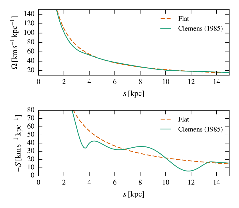
Figure 1: Two choices for the rotation curve discussed in the text (upper panel) and the corresponding velocity shear rate $S=s\mathrm{d}\Omega/\mathrm{d}s$ (lower panel): the Milky Way rotation curve obtained from CO observations by Clemens1985 (solid) and a simpler rotation curve given by Eq. (2) (dashed).

While the model can be applied to any galaxy, our choice of fiducial parameters is motivated by the Milky Way, with the disc rotation curve of Clemens1985. To illustrate the impact of the rotation curve on the magnetic field, we also consider a flat rotation curve (i.e., the rotational speed is nearly independent of $s$ at large distances from the disc axis),

$$V(s)=V_{0}\frac{1-\exp(-s/s_{*})}{1-\exp(-s_{0}/s_{*})}\,,$$ (2)

where $s_{0}$ is a reference galactocentric distance defined below, $V_{0}$ is the rotation speed at $s=s_{0}$ and we take $s_{*}=250\,{\rm pc}$. The two rotation curves and the corresponding velocity shear rates, $S=s\mathrm{d}\Omega/\mathrm{d}s$, are shown in Fig. 1.

The disc scale height is assumed to increase exponentially with the cylindrical radius (a flared disc),

$$h(s)=h_{0}\exp\left(\frac{s-s_{0}}{s_{\mathrm{h}}}\right)\,,$$ (3)

where we adopt a flaring length scale of $s_{\mathrm{h}}=5\,{\rm kpc}$, similar to that of the MW H i disc, and $s_{0}$ is the Galactocentric distance of the Sun (Kalberla2009). In our fiducial model, we adopted the characteristic height $h_{0}=0.5\,{\rm kpc}$, which is the scale height of the Lockman layer (Lockman1984; Dickey1990) near the Sun.

The radius of the dynamo-active part of the disc is chosen to be $s_{\mathrm{d}}=17\,{\rm kpc}$, similar to the radius of the supernova distribution in the MW (CaBh98). The fiducial values of the parameters that appear in the model (which are also input parameters for the galmag code) are shown in Table 1. Parameters of the halo are introduced in Section LABEL:PGH.

3.2 Thin-disc dynamos

In terms of cylindrical coordinates $(s,\phi,z)$, the radial and azimuthal components of the axisymmetric $\alpha^{2}\omega$-dynamo equation (1) can be written as

$$\frac{\partial B_{s}}{\partial t} =-\frac{\partial(\alpha B_{\phi})}{\partial z}+\beta\frac{\partial^{2}B_{s}}{\partial z^{2}}+\beta\frac{\partial}{\partial s}\left[\frac{1}{s}\frac{\partial(sB_{s})}{\partial s}\right],$$ (4)

$$\frac{\partial B_{\phi}}{\partial t} =SB_{s}+\frac{\partial(\alpha B_{s})}{\partial z}+\beta\frac{\partial^{2}B_{\phi}}{\partial z^{2}}+\beta\frac{\partial}{\partial s}\left[\frac{1}{s}\frac{\partial(sB_{\phi})}{\partial s}\right],$$ (5)

where $S=s\,\partial\Omega/\partial s$ is the velocity shear due to differential rotation. We do not exhibit the equation for $B_{z}$ since, in a thin disc, it decouples from the equations shown and can be solved separately (equivalently, $B_{z}$ can be derived from $\nabla\cdot\bm{B}=0$).

It is convenient to use dimensionless variables, denoted with tilde,

$$\widetilde{s}=s/s_{0}\qquad\text{and}\qquad\widetilde{z}=z/h_{0}\,,\quad\text{with }\;h_{0}=h(s_{0})\,,$$ (6)

where $s_{0}$ is the reference cylindrical radius within the disc – for example, $s_{0}=s_{\odot}\approx 8.5\,{\rm kpc}$ is a convenient choice in the MW. Using different length units across and along the disc allows us to make the disc thinness explicit and quantified with the (small) aspect ratio

$$\epsilon=h_{0}/s_{0}\,.$$ (7)

The large-scale velocity is measured in the units of a characteristic rotational speed $V_{0}=V(s_{0})$,

$$\widetilde{\bm{V}}=\frac{\bm{V}}{V_{0}}\,,\quad\widetilde{\Omega}=\Omega\frac{s_{0}}{V_{0}}\,.$$ (8)

Velocity shear due to differential rotation is non-dimensionalised similarly,

$$\widetilde{S}=\frac{S}{S_{0}}\,,\text{ with }S_{0}=S(s_{0})\,.$$ (9)

The unit of time is the turbulent magnetic diffusion time across the disc. With $\beta_{\mathrm{d}}$ the turbulent magnetic diffusivity in the disc, the dimensionless time is

$$\widetilde{t} =t\beta_{\mathrm{d}}/h_{0}^{2}\,.$$ (10)

The magnitude of the $\alpha$-effect can be estimated as

$$\alpha\simeq\min\left(l^{2}\Omega/h,v\right)\,,$$ (11)

where $l$ and $v$ are the turbulent scale and speed, and the corresponding fiducial value is used to non-dimensionalise $\alpha$:

$$\widetilde{\alpha}=\frac{\alpha}{\alpha_{0}}\,,\quad\alpha_{0}=\frac{l^{2}V_{0}}{h_{0}s_{0}}\,.$$ (12)

The magnitude of $\alpha$ cannot exceed $\alpha=v$ because it is a measure of the helical part of the turbulent flow speed, hence $\alpha/v$ cannot exceed unity. This limit is usually important only in the central parts of galaxies (where the thin-disc approximation does not apply anyway). Equation (11) gives the magnitude of $\alpha$ and its dependence on $s$ through the variations of $\Omega$ and $h$ with $s$. It is expected that $\alpha$ is an odd function of $z$. GZER08a; GEZR08b and BGE15 confirm this and discuss the dependence of $\alpha$ on $z$ in numerical simulations of the supernova-driven interstellar medium. We adopt a factorised form for $\alpha(s,z)$,

$$\widetilde{\alpha}(s,z)=\frac{\widetilde{\Omega}(s)}{\widetilde{h}(s)}a(z)\,,\qquad\text{where}\qquad a(-z)=-a(z)\,,$$ (13)

where we assume that $l$, in Eqs (11) and (12), is independent of $s$. The model can be generalised straightforwardly to more general forms of $\alpha(s,z)$.

When galactic outflow is neglected, the dynamo is fully characterised by two dimensionless control parameters that quantify the intensity of the mean magnetic induction due to helical turbulence and differential rotation, respectively:

$$R_{\alpha\text{d}}=\frac{h_{0}\alpha_{0}}{\beta_{\mathrm{d}}}=\frac{l^{2}V_{0}}{s_{0}\beta_{\mathrm{d}}}\,,\quad R_{\omega\text{d}}=\frac{h_{0}^{2}S_{0}}{\beta_{\mathrm{d}}}\,,$$ (14)

where the subscript ‘d’ refers to the disc (similar parameters are defined slightly differently in the halo – see Section LABEL:sec:SDS).

In terms of dimensionless variables, Eqs. (4) and (5) reduce to

$$\frac{\partial B_{s}}{\partial\widetilde{t}} =-R_{\alpha\text{d}}\frac{\partial(\widetilde{\alpha}B_{\phi})}{\partial\widetilde{z}}+\frac{\partial^{2}B_{s}}{\partial\widetilde{z}^{2}}+\epsilon^{2}\frac{\partial}{\partial\widetilde{s}}\left[\frac{1}{\widetilde{s}}\frac{\partial(\widetilde{s}B_{s})}{\partial\widetilde{s}}\right],$$ (15)

$$\frac{\partial B_{\phi}}{\partial\widetilde{t}} =R_{\omega\text{d}}\widetilde{S}B_{s}+R_{\alpha\text{d}}\frac{\partial(\widetilde{\alpha}B_{s})}{\partial\widetilde{z}}+\frac{\partial^{2}B_{\phi}}{\partial\widetilde{z}^{2}}+\epsilon^{2}\frac{\partial}{\partial\widetilde{s}}\left[\frac{1}{\widetilde{s}}\frac{\partial(\widetilde{s}B_{\phi})}{\partial\widetilde{s}}\right].$$ (16)

It is now clear that the solutions are fully determined by $R_{\alpha\text{d}}$, $R_{\omega\text{d}}$, $\widetilde{S}(s)$, $\widetilde{\alpha}(s)$ and $\epsilon$.

In a thin disc, the magnetic field distribution along $z$ is established over a time scale $h^{2}/\beta_{\mathrm{d}}\simeq 5\times 10^{8}\,{\rm yr}$ which is $\epsilon^{-2}=(s_{0}/h_{0})^{2}$ times shorter than the time scale at which the radial distribution evolves, $s_{0}^{2}/\beta_{\mathrm{d}}$. Because of this difference, the radial derivatives in Eqs. (15) and (16) have $\epsilon^{2}$ as a factor. Therefore, the magnetic field distribution in a thin disc can be represented as a local solution (at a given galactocentric distance $s$), $\bm{b}(z;s)$, modulated by an envelope $Q(s)$. The local solution also depends on $s$ since $\alpha$, $S$ and $h$ vary with $s$, but this variation is parametric. It is convenient to normalise the local solution to unit surface magnetic energy density, $\int_{-h}^{h}|\bm{b}|^{2}\,\mathrm{d}z=1$, at all values of $s$: then $Q(s)$ represents magnetic field strength at the galactocentric radius $s$ (an envelope of the local solutions). Thus, asymptotic solutions of Eqs. (15) and (16) for $\epsilon\ll 1$ have the form

$$\bm{B}(s,z,t)=\exp(\Gamma t)\,Q(s)\,\bm{b}(z;s)\,.$$ (17)

The magnetic field varies exponentially with time at a rate $\Gamma$ in the kinematic dynamo stage. In a saturated thin-disc dynamo, the solution has a similar form but with $\Gamma=0$ (PSS93). The local solution is discussed in Section 3.3, whereas Section 3.4 presents the radial solution $Q(s)$.

To simplify the notation, we use exclusively the dimensionless variables with the tilde suppressed in the remaining part of this section unless otherwise stated.

3.3 Local solutions

Governing equations for the local solution, $\bm{b}=\exp{(\gamma t)}\,(b_{s},b_{z})$, follow from Eqs. (15) and (16) when we put $\epsilon=0$:

$$\gamma(s)b_{s} =-R_{\alpha\text{d}}\frac{\partial}{\partial z}\left[\alpha(s,z)b_{\phi}\right]+\frac{\partial^{2}b_{s}}{\partial z^{2}}\,,$$ (18)

$$\gamma(s)b_{\phi} =R_{\omega\text{d}}S(s)b_{s}+\frac{\partial^{2}b_{\phi}}{\partial z^{2}}+R_{\alpha\text{d}}\frac{\partial}{\partial z}\left[\alpha(s,z)b_{s}\right]\,.$$ (19)

To allow for the disc flaring, we introduce the following new variables:

$$\widehat{z}=\frac{z}{h(s)}\,,\quad\widehat{b}_{s}=\frac{b_{s}}{R_{\alpha\text{d}}\Omega(s)}\quad\text{and}\quad\widehat{\gamma}=\gamma(s)\,h^{2}(s)\,.$$ (20)

Since $R_{\alpha\text{d}}\ll R_{\omega\text{d}}$ at $s\gtrsim 1\,{\rm kpc}$ in most spiral galaxies, we can omit the term proportional to $R_{\alpha\text{d}}$ in Eq. (19), thus obtaining the $\alpha\omega$-dynamo approximation:

$$\widehat{\gamma}(s)\widehat{b}_{s} =-\frac{\partial}{\partial\widehat{z}}\left[a(z)b_{\phi}\right]+\frac{\partial^{2}\widehat{b}_{s}}{\partial\widehat{z}^{2}}\,,$$ (21)

$$\widehat{\gamma}(s)b_{\phi} =\mathcal{D}(s)\widehat{b}_{s}+\frac{\partial^{2}b_{\phi}}{\partial\widehat{z}^{2}}\,,$$ (22)

where $a(z)$, the $z$-dependent part of $\alpha(s,z)$, is defined in Eq (13) and $\mathcal{D}(s)$, the local dynamo number, includes the radial variation of the dynamo parameters:

$$\mathcal{D}(s)=R_{\alpha\text{d}}R_{\omega\text{d}}\,\Omega(s)S(s)h^{2}(s)\,.$$ (23)

It is also convenient to introduce the local (in galactocentric radius) values of $R_{\alpha\text{d}}$ and $R_{\omega\text{d}}$,

$$\mathcal{R}_{\alpha}(s)=R_{\alpha\text{d}}\Omega(s)\,,\quad\mathcal{R}_{\omega}(s)=R_{\omega\text{d}}S(s)h^{2}(s)\,,$$ (24)

so that $\mathcal{D}=\mathcal{R}_{\alpha}\mathcal{R}_{\omega}$. The normalisation condition for the local solution reduces to

$$\int_{-1}^{1}\left(|\widehat{b}_{s}|^{2}+|{b}_{\phi}|^{2}\right)\,\mathrm{d}\widehat{z}=1\,,$$ (25)

where we have neglected $\widehat{b}_{z}$ because this component of magnetic field is, on average, weaker than the other two. To this order in $\epsilon$, $b_{z}$ does not enter the equations for $b_{s}$ and $b_{\phi}$ and can be solved for separately. The result can be shown to be identical to that obtained from $\nabla\cdot\bm{B}=0$.

The vacuum boundary conditions are

$$\widehat{b}_{s}=b_{\phi}=0\quad\text{at}\quad\widehat{z}=\pm 1\,.$$ (26)

Since $a(z)$ is an odd function of $z$, solutions of Eqs. (21) and (22) split into two independent classes, even and odd in $z$ (or quadrupolar and dipolar, respectively). These can be distinguished using the symmetry conditions at the galactic mid-plane,

$$\frac{\partial\widehat{b}_{s}}{\partial\widehat{z}} =\frac{\partial b_{\phi}}{\partial\widehat{z}}=b_{z}=0\quad\text{at\ }z=0\quad\text{(even\ parity)},$$ (27)

$$\widehat{b}_{s} =b_{\phi}=\frac{\partial b_{z}}{\partial\widehat{z}}=0\quad\text{at\ }z=0\quad\text{(odd\ parity)}.$$ (28)

Approximate solutions for both parity families can be obtained in the form of an expansion over the free-decay modes obtained as solutions of Eqs. (21) and (22) for $a(z)=\mathcal{D}(s)=0$. The procedure is discussed in detail by ShSo08 and CSSS14, and here we only provide the results.

From Eqs. (21)–(27), we obtain the following approximate solutions of quadrupolar symmetry, for ${a(\widehat{z})=\sin(\pi\widehat{z}/2)}$:

$$b_{s}(z;s) \approx\mathcal{R}_{\alpha}{(s)}K_{0}(s)\left[\cos\frac{\pi z}{2h(s)}+\frac{3\sqrt{-\mathcal{D}(s)}}{4\pi^{3/2}}\cos\frac{3\pi z}{2h(s)}\right]\,,$$ (29)

$$b_{\phi}(z;s) \approx-2K_{0}{(s)}\sqrt{-\frac{\mathcal{D}(s)}{\pi}}\cos\frac{\pi z}{2h(s)}\,,$$ (30)

$$\gamma(s) \approx\frac{1}{h^{2}(s)}\left[-\frac{\pi^{2}}{4}+\frac{1}{2}\sqrt{-\pi\mathcal{D}(s)}\right]\,,$$ (31)

where

$$K_{0}{(s)}=\left[1-\frac{4\mathcal{D}(s)}{\pi}-\frac{9\mathcal{D}(s)}{16\pi^{3}}\right]^{-1/2}$$ (32)

is the normalization factor obtained using Eq. (25). These solutions are shown in Fig. 2. Equation (31) provides the critical value of the local dynamo number required for the local amplification and maintenance of the magnetic field: $\gamma\geq 0$ for $\mathcal{D}\leq\mathcal{D}_{\mathrm{c}}\approx-\pi^{3}/4\approx-8$. Other choices of the functional form of $a(\widehat{z})$ lead to slightly different values of the critical dynamo number (e.g. $-11$ for $a=z$), but the difference hardly has any practical consequences.

In the odd-parity solutions, the term proportional to $(-\mathcal{D})^{1/2}$ in $b_{s}$ vanishes for $a(\widehat{z})=\sin(\pi\widehat{z}/2)$. Therefore, it is more convenient to use a similar solution with $a(z)=\widehat{z}$ that satisfies the symmetry condition (28), here written to the lowest order in $(-\mathcal{D})^{1/2}$:

$$b_{s}(z;s) \approx K_{1}{(s)}\mathcal{R}_{\alpha}{(s)}\sqrt{2}\sin\frac{\pi z}{h(s)}\,,$$ (33)

$$b_{\phi}(z;s) \approx-2K_{1}{(s)}\sqrt{-\mathcal{D}(s)}\sin\frac{\pi z}{h(s)}\,,$$ (34)

$$\gamma(s) \approx\frac{1}{h^{2}(s)}\,,$$ (35)

with

$$K_{1}{(s)}=\left[1-4\mathcal{D}(s)\right]^{-1/2}\,.$$ (36)

The dipolar modes can be excited, $\gamma\geq 0$, for $\mathcal{D}\leq-2\pi^{4}\approx-195$, a threshold much higher than for the quadrupolar modes. This is true for any plausible form of $a(\widehat{z})$ and explains the predominance of quadrupolar magnetic fields in thin discs.

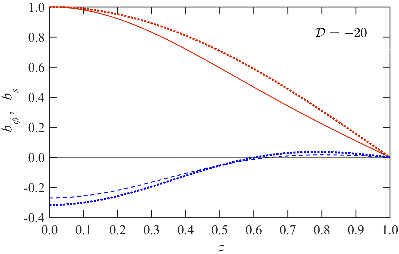
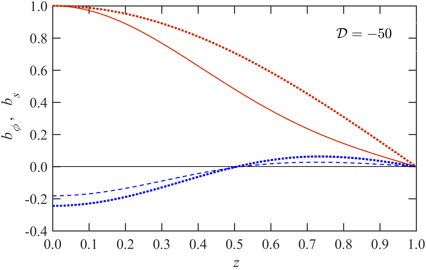
Figure 2: Comparison of the local quadrupolar eigenfunctions for $\mathcal{D}=-20$ (upper panel) and $-50$ (middle panel) obtained from numerical solution of the local equations (21) and (22) with the approximate eigenfunctions (29) and (30): $b_{\phi}$ from the numerical solution are shown solid (red) and $b_{s}$, dashed (blue); their approximate counterparts are shown with dotted curves of the matching colour. The eigenfunctions are normalised to $b_{\phi}(0)=1$. The bottom panel shows the numerical (black, solid) and approximate, Eq. (31) (red, dashed), solutions for the local growth rate as a function of the local dynamo number.

The local solutions are derived, formally, for $|\mathcal{D}|\ll 1$ but they remain reasonably accurate for $|\mathcal{D}|$ as large as about 50 or more (2JCBS14). We compare in Fig. 2 the local quadrupolar eigenfunctions obtained from numerical solution of Eqs. (21) and (22) with the approximate solutions (29)–(31) for $\mathcal{D}=-20$ and $-50$, values typical of the main parts of spiral galaxies (see Fig. 3).

The local eigenfunctions presented above are approximate solutions of the mean-field dynamo equations. However, the functional basis of these solutions, the free-decay modes, can be used as a complete functional basis to represent any magnetic field configuration. The free-decay modes are solutions of Eqs. (21) and (22) with $a(z)=0$ and $\mathcal{D}(s)=0$, so that the equations decouple and can easily be solved. Normalised as in Eq. (25), the dipolar and quadrupolar free-decay eigenfunctions and eigenvalues (identified with superscripts $d$ and $q$, respectively) have the following respective forms with $n=1,2,3,\ldots$:

$$\bm{b}_{n}^{(\text{d})}=\pmatrix{\sin}(\pi n\widehat{z})\\ 0\,,\quad\bm{b}_{n}^{(\text{d})\prime}=\pmatrix{0}\\ \sin(\pi n\widehat{z})\,,\quad\widehat{\gamma}_{n}^{(\text{d})}=-\pi^{2}n^{2}\,,$$ (37)

(38)

(39)

,bn(q)′=(0) cos[π(n-12)^z] , ^γn(q)&=-π2(n-12)2.

The free-decay disc modes are double degenerate as two orthogonal modes of the same parity (distinguished by prime) correspond to each eigenvalue.

3.4 Radial solution

When Eq. (17) is substituted into Eqs. (15) and (16), and Eqs. (18) and (19) are allowed for, equations for both $B_{s}$ and $B_{\phi}$ reduce to the same equation for $Q(s)$, that is,

$$\epsilon^{2}\frac{\partial}{\partial s}\left[\frac{1}{s}\frac{\partial}{\partial s}(sQ)\right]+[\gamma(s)-\Gamma]Q=0\,,$$ (40)

where $\gamma(s)$ is the local growth rate obtained as a part of the local solution, (31) or (35). This equation applies to both even and odd local solutions, and to both $\alpha^{2}\omega$ and $\alpha\omega$-dynamos, that is, with and without the term proportional to $R_{\alpha\text{d}}$ in Eq. (19). The boundary conditions adopted are

$$Q(0)=Q(s_{\mathrm{d}})=0\,.$$ (41)

The condition at $s=0$ follows from axial symmetry, whereas that at the outer boundary of the dynamo-active region $s=s_{\mathrm{d}}$ is adopted for the sake of simplicity.

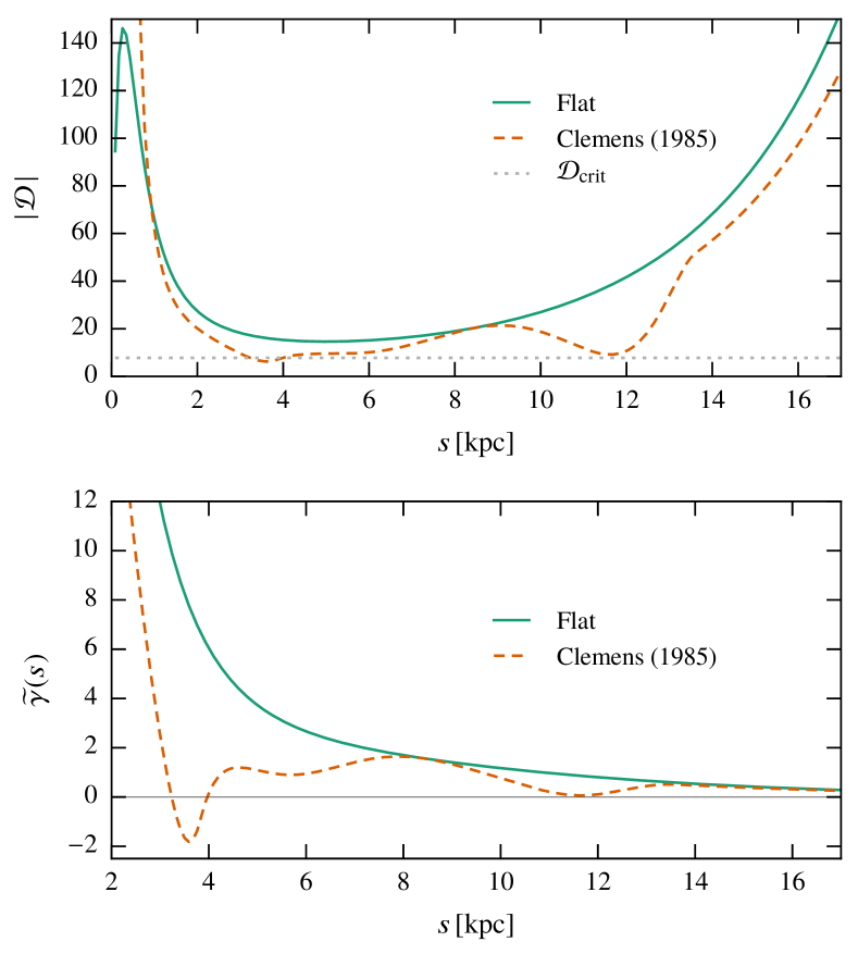
Figure 3: Radial profiles of the local dynamo number (upper panel) and the local growth rate of the quadrupolar solutions (lower panel) for the flat rotation curve (2) (solid) and for the MW rotation curve of Clemens1985 (dashed). In the upper panel, the critical dynamo number $\mathcal{D}_{\mathrm{c}}\approx-\pi^{3}/4$ is shown dotted for reference.

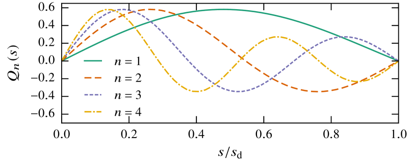
Figure 4: Four leading eigenmodes $Q_{n}(s)$ of the radial equation (40) given by Eq. (43).

When $\Omega(s)$ and $h(s)$ are known, the global growth rate $\Gamma$ and the radial distribution of the magnetic field strength $Q(s)$ can be obtained by solving Eq. (40) numerically. However, for our present purposes it is more useful to obtain an approximate analytical solution for $Q(s)$. This allows faster computations at the cost of an additional approximation. When the magnetic field model is used in Bayesian analyses, the computation speed is of primary importance.

To obtain a simple analytical solution of Eq. (40), consider $\gamma$ to be a constant, $\gamma=\gamma_{0}$, within the disc radius, $s<s_{\mathrm{d}}$, and zero outside,

$$\gamma(s)=\cases{\gamma}_{0}\,$$ (42)

&0≤s<sd, 0,s≥sd.

A suitably averaged value of $\gamma(s)$ within the disc can be adopted for $\gamma_{0}$. The relevance of this approximation depends on the specific case, particularly the rotation curve and the rate of the disc flaring, as shown in Fig. 3. The inner parts of the disc, $s\lesssim 1\,{\rm kpc}$, should be disregarded since the thin-disc approximation is not applicable there. At $s\gtrsim 1\,{\rm kpc}$, the approximation $\gamma(s)=\mathrm{const}$ does not appear unreasonable, especially for the Milky Way rotation curve, as shown in the lower panel of Fig. 3.

For $\gamma(s)$ of Eq. (3.4), equation (40) with boundary conditions (41) can be solved to yield the eigensolutions

$$Q_{n}(s) =J_{1}\left(k_{n}s/s_{\mathrm{d}}\right)\,,\qquad n=1,2,3,\ldots\,,$$ (43)

$$\Gamma_{n} =\gamma_{0}-\epsilon^{2}k_{n}^{2}\,,$$ (44)

where $J_{1}(x)$ is the standard Bessel function (of order one) and $k_{n}\approx\leavevmode\nobreak\ 3.83,7.02,10.17,\ldots$ are its zeros, thus, $J_{1}(k_{n})=0$. The first four modes of $Q_{n}(s)$ are shown in Fig. 4. Independently of the form of $\gamma(s)$, the lowest radial mode, $Q_{1}(s)$, is sign-constant but $Q_{n}(s)$ has $n-1$ zeros, and thus the scale of variation of $Q_{n}(s)$ decreases with $n$. This feature of the solution is responsible for the reversals of the large-scale magnetic field discussed in Section LABEL:FRAGR.

The evolving radial distribution of magnetic field is obtained as a superposition of the eigensolutions of Eq. (40):

$$Q(s,t)=\sum_{n=1}^{\infty}C_{n}\mathrm{e}^{\Gamma_{n}t}Q_{n}(s)\,,$$ (45)

where, in the context of dynamo models, the coefficients $C_{n}$ are determined by the initial conditions. Alternatively, the eigenfunctions $Q_{n}(s)\bm{b}(z;s)$ can be used as the basis functions to represent a given magnetic field with $\exp(\Gamma_{n}t)$ absorbed into $C_{n}$. The set of radial eigenfunctions $Q_{n}$ is complete, so that any radial distribution of magnetic field can be represented in this form. The only constraint on the form of the solution is due to the fact that the set of the local solutions $\bm{b}$ is incomplete. Nevertheless, a wide class of magnetic field distributions along $z$ can be represented as a superposition of various quadrupolar and dipolar local modes, so that the lack of the functional completeness of the local solutions is not likely to be restrictive in practice. Otherwise, the complete set of local free-decay modes $\bm{b}_{m}^{\text{(q,d})}(z;s)$ of Eqs. (37)–(3.3) can be used instead of the local dynamo solutions to construct a more general expansion over a complete set of basis functions of the form

$$\bm{B}(s,z)=\sum_{m=1}^{\infty}\sum_{n=1}^{\infty}C_{mn}Q_{n}(s)\bm{b}_{m}^{\text{(q,d})}(z;s)\,,$$

which can be used to parametrise (in terms of the coefficients $C_{mn}$) an arbitrary magnetic field that does not need to be a solution of the dynamo equations.

3.5 Vertical magnetic field

The axially symmetric vertical component of the magnetic field, $B_{z}$, can be obtained from

$$\nabla\cdot\bm{B}=\frac{1}{s}\frac{\partial}{\partial s}(sB_{s})+\frac{\partial B_{z}}{\partial z}=0\,,$$ (46)

using $B_{s}(s,z)=b_{s}(z;s)Q(s)$ from Eq. (29) or (33), and Eq. (43). We have assumed that $\gamma_{0}=\mathrm{const}$ to derive the simple form Eq. (43), implying $\mathcal{D}=\mathrm{const}$. It is therefore justifiable to neglect the dependence of $\mathcal{D}$, $\Omega$ and $h$ on $s$ when differentiating $B_{s}$ in (46) and only retain the dependence of $Q$ on $s$ (this simplification can easily be relaxed if required). By virtue of linearity, Eq. (46) can be solved for each radial mode $n$ separately:

$$-\frac{\partial B_{z}^{(n)}}{\partial z} =\frac{1}{s}\frac{\partial}{\partial s}(sB_{s}^{(n)})=\mathcal{R}_{\alpha}K_{0}C_{n}\frac{1}{s}\frac{\mathrm{d}}{\mathrm{d}s}\left[sJ_{1}(k_{n}s/s_{\text{d}})\right]$$

$$\times\left(\cos\frac{\pi z}{2h(s)}+\frac{3}{4\pi^{3/2}}\sqrt{-\mathcal{D}(s)}\cos\frac{3\pi z}{2h(s)}\right)\,.$$ (47)

Then, for the quadrupolar parity,

$$B_{z}^{(n)} =-{\mathcal{R}_{\alpha}K_{0}C_{n}}\frac{k_{n}}{s_{\text{d}}}J_{0}\left(\frac{k_{n}s}{s_{\text{d}}}\right)$$

$$\mbox{}\quad\times\int_{0}^{z}\!\left(\cos\frac{\pi z^{\prime}}{2h}+\frac{3\sqrt{-\mathcal{D}}}{4\pi^{3/2}}\cos\frac{3\pi z^{\prime}}{2h}\right)\mathrm{d}z^{\prime}$$ (48)

where the dependence of $\mathcal{R}_{\alpha}$ $\mathcal{D}$, $h$ and $K_{0}$ on $s$ should be allowed for.

3.6 Magnetic field in the disc

We can now collect the solutions from Sections 3.3, 3.4 and 3.5 to write the approximate solution of the dynamo equation (evolving or at a fixed time) for a thin disc as a sum of $N_{r}$ radial eigenmodes,

$$\pmatrix{B}$$ (49)

Bϕ Bz