Abstract

We investigate a time-dependent spatial vector-host epidemic model with non-coincident domains for the vector and host populations. The host population resides in small non-overlapping sub-regions, while the vector population resides throughout a much larger region. The dynamics of the populations are modeled by a reaction-diffusion-advection compartmental system of partial differential equations. The disease is transmitted through vector and host populations in criss-cross fashion. We establish global well-posedness and uniform a prior bounds as well as the long-term behavior. The model is applied to simulate the outbreak of bluetongue disease in sheep transmitted by midges infected with bluetongue virus. We show that the long-range directed movement of the midge population, due to wind-aided movement, enhances the transmission of the disease to sheep in distant sites.

2000 Mathematics Subject Classification: 92A15, 35B40, 35M20, 35K57, 35Q92.

Keywords: vector-host, reaction-diffusion-advection, asymptotic behavior, bluetongue.

1 Introduction

Many diseases, such as malaria, dengue fever, Zika, Chagas disease in humans, and bluetongue disease in sheep and other ruminants, are transmitted in criss-cross fashion between vectors and hosts. Vectors, such as mosquitoes, fleas, ticks, and midges, transmit microbial disease agents to animal and human host populations. Susceptible vectors become infected by interaction with infected hosts, and infected vectors transmit the disease to susceptible hosts. Mathematical models for the spatial spread of such diseases have been developed by many authors, e.g. [3, 5, 10, 18, 19, 20, 21, 23, 24, 25, 26, 48].

In this paper, we investigate a vector-host model describing the spatio-temporal spread of an epidemic disease, with host populations residing in non-overlapping small domains, and vectors residing in a much larger region. We assume that the host population has both a random spatial movement and a directed spatial movement. We will show that the spread of a vector-host epidemic disease over a large geographic region can result from an outbreak in a relatively small host subregion, by directed long-range movement of vectors to distant host subregions.

The directed movement can result from external forces such as wind-aided movement. The role of wind-aided movement in the transmission of disease has been studied by many researchers, including [6, 8, 15, 38, 33, 43, 42]. In [42] the authors study the wind-borne transportation of Highly Pathogenic Avian influenza virus between farms, where the movement of pathogen particles is described by a Gaussian Plume Model, which is essentially an advection-diffusion model. In [43], the authors use stochastic simulations to study the impact of the movement of midges due to wind on the spread of bluetongue virus in Europe. In [8], Burgin et al. the authors use an atmospheric dispersion model to study the impact of wind on the spread of bluetongue disease in sheep.

The organization of this paper is as follows: in Section 2 we analyze a general model of this class of epidemics, in which both vectors and hosts are diffusing in their domains; in Section 3 we analyze a special case in which only the vectors are diffusing in their domain; in Section 4 we apply the results in Section 3 to an outbreak of bluetongue disease in sheep. The results of Section 4 address the issue of the recent spread of bluetongue disease in Europe.

2 The Model

2.1 The vector population model

The vector habitat is considered to be a region sufficiently large to contain numerous sub regions which contain host populations. We shall depart from the standard practice of using bounded regions to define species habitats and simply define the vector habitat as $\displaystyle\mathbb{R}^{2}$. We assume that the spatially distributed vector population $\displaystyle V(x,t)$ is subject to logistic demographics with spatially dependent linear birth term of the form $\displaystyle\beta(x)V(x,t)$ and a quadratic self-limiting term of the form $\displaystyle-m(x)V^{2}(x,t)$. Dispersion of the vectors is modeled by diffusion and advection with diffusion describing the natural movement of the vectors and advection accounting for the effective of the wind. These considerations give rise to the following reaction-diffusion-advection type equation:

$$\left\{\begin{array}[]{lll}\frac{\partial V}{\partial t}-\triangledown\cdot D(x)\triangledown V+\overrightarrow{C}(x,t)\cdot\triangledown V=\beta(x)V-m(x)V^{2},&\ \ \ x\in\mathbb{R}^{2},\ t>0,\vskip 6.0pt plus 2.0pt minus 2.0pt\\ V(x,0)=V_{0}(x),&\ \ \ x\in\mathbb{R}^{2}.\end{array}\right.$$ (2.1)

Eq. (2.1) is a classic semi-linear reaction-diffusion-advection equation commonly known as a convective Fisher-Kolmogorov equation. Fisher-Kolmogorov equations [17] first introduced in the 1930s remain of active interest and arise in a variety of applications. We assume that the diffusion coefficient $\displaystyle D(x)$ is up to order 2 uniformly bounded and continuous, strictly positive on $\displaystyle\mathbb{R}^{2}$, i.e.

• $\displaystyle D\in C_{b}^{2}(\mathbb{R}^{2})$;

• There exist $\displaystyle D_{m},D_{M}>0$ such that $\displaystyle D_{m}\leq D(x)\leq D_{M}$ for all $\displaystyle x\in\mathbb{R}^{2}$.

We make the following assumptions on the velocity field $\displaystyle\overrightarrow{C}(x,t)$:

• $\displaystyle\overrightarrow{C}\in C(\mathbb{R}_{+};C_{b}^{1}(\mathbb{R}^{2}))$;

• $\displaystyle\triangledown\cdot\overrightarrow{C}(\cdot,t)=0$ for all $\displaystyle t\geq 0$.

The terms $\displaystyle\beta(x)V$ and $\displaystyle m(x)V^{2}$ represent spatially dependent birth and logistic mortality rates of the vector population, respectively. We require that

• $\displaystyle\beta(x)\geq 0$ for all $\displaystyle x\in\mathbb{R}^{2}$, and $\displaystyle\beta\in C_{b}^{1}(\mathbb{R}^{2})$ with $\displaystyle\|\beta\|_{\infty,\mathbb{R}^{2}}\leq\beta^{*}<\infty$ for some positive constant $\displaystyle\beta^{*}$;

• $\displaystyle m\in C_{b}^{1}(\mathbb{R}^{2})$, and there exist positive constants $\displaystyle m_{*},m^{*}$ such that $\displaystyle m_{*}\leq m(x)\leq m^{*}$ for all $\displaystyle x\in\mathbb{R}^{2}$.

We make the following assumption on the initial data:

• $\displaystyle V_{0}(x)\geq 0$ for all $\displaystyle x\in\mathbb{R}^{2}$, and $\displaystyle V_{0}\in C_{b}(\mathbb{R}^{2})\cap L^{1}(\mathbb{R}^{2})$.

Let $\displaystyle Q(s,t)$ be the space-time cylinder $\displaystyle\mathbb{R}^{2}\times(s,t)$.

The following theorem guarantees the global well-posedness of solutions to (2.1).

Theorem 2.1

Assume that (A1)-(A7) hold. Then there exists a unique classical global solution $\displaystyle V(x,t)$ of (2.1) such that

$$0\leq V(x,t)\leq\max\left\{\frac{\beta^{*}}{m_{*}},\|V_{0}\|_{\infty,\mathbb{R}^{2}}\right\},\ \ \ \text{for all }(x,t)\in Q(0,\infty).$$

Proof. Local well-posedness can be obtained using a Green’s function argument. The uniform a priori bound and the non-negativity follow from the fact that $\displaystyle(0,\beta^{*}/m_{*})$ is an invariant rectangle [46]. The presence of the uniform a priori bound guarantees a global solution [4].   

Throughout this paper, we suppose that $\displaystyle\Omega$ is a bounded domain in $\displaystyle\mathbb{R}^{2}$ with smooth boundary $\displaystyle\partial\Omega$ such that $\displaystyle\Omega$ lies locally on one side of $\displaystyle\partial\Omega$. We define an operator $\displaystyle T:H^{1}(\Omega)\rightarrow H^{1}(\Omega)$ by

$$T(u):=\triangledown\cdot D\triangledown u+\beta u,\ u\in H^{2}(\Omega)\cap H_{0}^{1}(\Omega),$$

It is well-known that the principal eigenvalue of $\displaystyle T$ has the following variational characterization:

$$\max_{u\in H_{0}^{1}(\Omega),\|u\|_{2,\Omega}=1}\int_{\Omega}(-D(x)|\triangledown u(x)|^{2}+\beta(x)u^{2}(x))dx.$$

We can prove the following:

Theorem 2.2

Suppose that (A1)-(A2) and (A5)-(A6) hold, $\displaystyle\overrightarrow{C}=0$, and $\displaystyle V_{0}$ is nontrivial. If the principal eigenvalue of $\displaystyle T$ is positive, then for any $\displaystyle\Omega^{\prime}\subset\subset\Omega$, there exist $\displaystyle\epsilon_{0}>0$ independent on $\displaystyle V_{0}$ such that the solution $\displaystyle V(x,t)$ of (2.1) satisfies $\displaystyle V(x,t)>\epsilon_{0}$ for all $\displaystyle x\in\bar{\Omega}^{\prime}$ and $\displaystyle t>t_{0}$ for some $\displaystyle t_{0}>0$.

Proof. Since the principal eigenvalue of $\displaystyle T$ is positive, there is a unique positive solution $\displaystyle u$ of

$$\left\{\begin{array}[]{lll}\triangledown\cdot D\triangledown u+\beta u-mu^{2}=0,&x\in\Omega,\\ u=0,&x\in\partial\Omega.\end{array}\right.$$ (2.2)

For any $\displaystyle v_{0}\in C_{0}(\bar{\Omega})$ that is nonnegative and nontrivial, let $\displaystyle v(x,t)$ be the solution of the problem

$$\left\{\begin{array}[]{lll}v_{t}=\triangledown\cdot D\triangledown v+\beta v-mv^{2},&x\in\Omega,t>0,\\ v(x,t)=0,&x\in\partial\Omega,t>0,\\ v(x,0)=v_{0},&x\in\Omega.\end{array}\right.$$ (2.3)

Then, we have (see, e.g. [9])

$$\lim_{t\rightarrow\infty}\|v(\cdot,t)-u\|_{\infty,\Omega}=0.$$ (2.4)

Suppose that $\displaystyle V_{0}$ is nontrivial. Then by the maximum principle, $\displaystyle V(x,t)>0$ for all $\displaystyle(x,t)\in Q(0,\infty)$. So without loss of generality, we may assume that $\displaystyle V_{0}(x)>0$ for all $\displaystyle x\in\Omega$. Let $\displaystyle v_{0}\in C_{0}(\bar{\Omega})$ such that $\displaystyle 0<v_{0}(x)<V_{0}(x)$ for all $\displaystyle x\in\Omega$. Then $\displaystyle V(x,t)$ is a super solution of (2.3). By the comparison principle, we have $\displaystyle V(x,t)>v(x,t)$ for all $\displaystyle x\in\Omega$ and $\displaystyle t>0$. Let $\displaystyle a=\min_{x\in\overline{\Omega^{\prime}}}u(x)$. By (2.4), there exists $\displaystyle t_{0}>0$ such that

$$V(x,t)>v(x,t)>\frac{a}{2}:=\epsilon_{0},\ \text{ for all }\ x\in\overline{\Omega^{\prime}}\ \text{ and }\ t>t_{0}.$$

 

For $\displaystyle r>0$, let $\displaystyle B_{r}$ be the closed disk in $\displaystyle\mathbb{R}^{2}$ of radius $\displaystyle r$ centered at the origin.

Corollary 2.3

Suppose that (A1)-(A2) and (A5)-(A6) hold and $\displaystyle\overrightarrow{C}=0$. If

$$\int_{\mathbb{R}^{2}}\beta(x)dx>\frac{\pi^{2}D_{M}}{2},$$ (2.5)

then for any $\displaystyle r>0$, there exist $\displaystyle\epsilon_{0}>0$ independent on $\displaystyle V_{0}$ and $\displaystyle t_{0}>0$ such that the solution $\displaystyle V(x,t)$ of (2.1) satisfies $\displaystyle V(x,t)>\epsilon_{0}$ for all $\displaystyle x\in B_{r}$ and $\displaystyle t>t_{0}$.

Proof. For each $\displaystyle a>0$, let $\displaystyle X_{a}=(-a,a)\times(-a,a)$. Let $\displaystyle\epsilon\in(0,1)$ be given. By the assumption (2.5), there exits $\displaystyle K>0$ such that

$$(1-\epsilon)\int_{X_{K}}\beta(x)dx>\frac{\pi^{2}D_{M}}{2},$$

and $\displaystyle B_{r}$ is a subset of $\displaystyle X_{K}$. In addition, there exists $\displaystyle\delta=\delta(\epsilon)\in(0,1)$ such that $\displaystyle 1-\epsilon\leq\sin^{2}(w)\leq 1$ whenever $\displaystyle|w-\pi/2|\leq\delta$. Let $\displaystyle L=\frac{\pi}{2\delta}K$. Then $\displaystyle L>K$ and $\displaystyle B_{r}$ is a subset of $\displaystyle X_{L}$. Moreover, one can check that $\displaystyle 1-\epsilon\leq\sin^{2}(\frac{\pi(x+L)}{2L})\leq 1$ whenever $\displaystyle|x|\leq K$.

Define

$$\phi(x)=\frac{1}{L}\sin(\frac{\pi(x_{1}+L)}{2L})\sin(\frac{\pi(x_{2}+L)}{2L})\ \text{ for }x=(x_{1},x_{2})\in X_{L}.$$

Then $\displaystyle\phi\in H^{1}_{0}(X_{L})$, $\displaystyle\|\phi\|_{2,X_{L}}=1$ and $\displaystyle\|\triangledown\phi\|_{2,X_{L}}=\frac{\pi}{\sqrt{2}L}$. It then follows that

$$\displaystyle\max_{u\in H_{0}^{1}(X_{L}),\|u\|_{2,X_{L}}=1}\int_{X_{L}}(-D(x)|\triangledown u(x)|^{2}+\beta(x)u^{2}(x))dx$$

$$\displaystyle\hskip 85.35826pt\geq\int_{X_{L}}(-d_{max}|\triangledown\phi(x)|^{2}+\beta(x)\phi^{2}(x))dx$$

$$\displaystyle\hskip 85.35826pt\geq-D_{M}\frac{\pi^{2}}{2L^{2}}+\int_{X_{K}}\beta(x)\phi^{2}(x)dx$$

$$\displaystyle\hskip 85.35826pt\geq-D_{M}\frac{\pi^{2}}{2L^{2}}+\frac{1-\epsilon}{L^{2}}\int_{X_{K}}\beta(x)dx>0.$$

Consequently, the principal eigenvalue of $\displaystyle T$ is positive, and the claim follows from Theorem 2.2.   

2.2 Vector host transmission

We assume that the host population is distributed between two distinct bounded sub-regions $\displaystyle\Omega_{1}$ and $\displaystyle\Omega_{2}$ of $\displaystyle\mathbb{R}^{2}$ that are in sufficiently close proximity to allow natural vector diffusion without the presence of the wind to drive the vector borne transmission of the pathogen from one field to another. Both $\displaystyle\Omega_{1}$ and $\displaystyle\Omega_{2}$ are assumed to have smooth boundaries $\displaystyle\partial\Omega_{1}$ and $\displaystyle\partial\Omega_{2}$ and to lie locally on one side of their boundaries. The sub-regions are non-overlapping and separated:

$$\Omega_{1}\cap\Omega_{2}=\emptyset\ \ \text{ and }\ \ dist(\Omega_{1},\Omega_{2})>0.$$

We let $\displaystyle H_{1}$ and $\displaystyle H_{2}$ denote the host populations which occupy $\displaystyle\Omega_{1}$ and $\displaystyle\Omega_{2}$ respectively, and assume that $\displaystyle H_{1}$ remains confined to $\displaystyle\Omega_{1}$ and $\displaystyle H_{2}$ remains confined to $\displaystyle\Omega_{2}$. We model the circulation in each of the subregions by an SEIR model. The susceptible class, $\displaystyle S_{j}$ for $\displaystyle j=1,2$, consists of individuals who are free of the pathogen. The exposed class, $\displaystyle E_{j}$ for $\displaystyle j=1,2$, consists of individuals who have been infected with the pathogen. However at this stage the disease is incubating and these individuals are not capable of transmitting the pathogen. The infected/infectious class, $\displaystyle I_{j}$ for $\displaystyle j=1,2$, consists of individuals who are capable of transmitting the disease. The removed class, $\displaystyle R_{j}$, for $\displaystyle j=1,2$, consists of individuals who have either perished from the disease or have recovered, and thereby gained immunity. The variables $\displaystyle S_{j}(x,t)$, $\displaystyle E_{j}(x,t)$, $\displaystyle I_{j}(x,t)$, $\displaystyle R_{j}(x,t)$ for $\displaystyle j=1,2$ represent the time dependent spatial densities in each of the subregions $\displaystyle\Omega_{j}$. The total population of each class in each subregion is given by integration over the subregion.

Susceptible hosts in each subregion are infected via contact with infected vectors. We model this by mass action force infection terms: $\displaystyle\sigma_{1}(x)S_{1}(x,t)V_{i}(x,t)$, $\displaystyle x\in\Omega_{1},t>0$, and $\displaystyle\sigma_{2}(x)S_{2}(x,t)V_{i}(x,t)$, $\displaystyle x\in\Omega_{2},t>0$. We assume that exposed hosts in either subregion become fully infected at constant rate $\displaystyle\lambda>0$, and that removal by death or recovery in either subregion occurs at a rate $\displaystyle\delta>0$.

The host population of each subregion remains confined to that subregion. The dispersion through each subregion is modeled by diffusion with the diffusivities of the susceptible and exposed hosts in subregions $\displaystyle\Omega_{1}$ and $\displaystyle\Omega_{2}$ given by $\displaystyle D_{11}(x)$ and $\displaystyle D_{12}(x)$. The dispersion of infected/infective hosts in $\displaystyle\Omega_{1}$ and $\displaystyle\Omega_{2}$ is modeled by $\displaystyle D_{21}(x)$ and $\displaystyle D_{22}(x)$.

Infected vectors can be recruited by means of contact with infected hosts in either of the two sub-regions. This process is modeled by the incidence term:

$$f(x,t,I_{1},I_{2},V_{s})=\left\{\begin{array}[]{lrl}\alpha_{1}(x)I_{1}V_{s},&x\in\bar{\Omega}_{1},t>0\\ \alpha_{2}(x)I_{2}V_{s},&x\in\bar{\Omega}_{2},t>0\\ 0,&x\in\mathbb{R}^{2}/\bar{\Omega}_{1}\cup\bar{\Omega}_{2},t>0.\end{array}\right.$$

We assume that the presence of the pathogen has no deleterious effect on the vectors.

The following equations model the vector-host populations:

• Vector Populations

  $$\left\{\begin{array}[]{lll}\frac{\partial}{\partial t}V_{s}=\triangledown\cdot D(x)\triangledown V_{s}-\overrightarrow{C}(x,t)\cdot\triangledown V_{s}+\beta(x)V-m(x)V_{s}V-f(x,t,I_{1},I_{2},V_{s}),\\ \hskip 325.215pt(x,t)\in Q(0,\infty),\\ \frac{\partial}{\partial t}V_{i}=\triangledown\cdot D(x)\triangledown V_{i}-\overrightarrow{C}(x,t)\cdot\triangledown V_{i}-m(x)V_{i}V+f(x,t,I_{1},I_{2},V_{s}),\\ \hskip 325.215pt(x,t)\in Q(0,\infty),\\ V_{s}(x,0)=V_{s0}(x),\ \ \ V_{i}(x,0)=V_{i0}(x),\ \ \ x\in\mathbb{R}^{2}.\end{array}\right.$$ (2.6)

• Host Populations

  $$\left\{\begin{array}[]{lll}\frac{\partial}{\partial t}S_{j}=\triangledown\cdot D_{1j}(x)\triangledown S_{j}-\sigma_{j}(x)S_{j}V_{i},\ \ \ (x,t)\in\Omega_{j}\times(0,\infty),\,j=1,2,\vskip 6.0pt plus 2.0pt minus 2.0pt\\ \frac{\partial}{\partial t}E_{j}=\triangledown\cdot D_{1j}(x)\triangledown E_{j}+\sigma_{j}(x)S_{j}V_{i}-\lambda E_{j},\ \ \ (x,t)\in\Omega_{j}\times(0,\infty),\,j=1,2,\vskip 6.0pt plus 2.0pt minus 2.0pt\\ \frac{\partial}{\partial t}I_{j}=\triangledown\cdot D_{2j}(x)\triangledown I_{j}+\lambda E_{j}-\delta I_{j},\ \ \ (x,t)\in\Omega_{j}\times(0,\infty),\,j=1,2,\vskip 6.0pt plus 2.0pt minus 2.0pt\\ \frac{\partial}{\partial n}S_{j}=\frac{\partial}{\partial n}E_{j}=\frac{\partial}{\partial n}I_{j}=0,\ \ \ (x,t)\in\partial\Omega_{j}\times(0,\infty),\,j=1,2,\vskip 6.0pt plus 2.0pt minus 2.0pt\\ S_{j}(x,0)=S_{j0}(x),\ \ \ E_{j}(x,0)=E_{j0}(x),\ \ \ I_{j}(x,0)=I_{j0}(x),\ \ \ \ x\in\Omega_{j},\,j=1,2.\end{array}\right.$$ (2.7)

The removed classes have no effect on the progress of the disease and do not appear in our system of equations. The homogeneous Neumann boundary conditions in (2.7) guarantee that the hosts remain confined to their habitats.

We further impose the following assumptions:

• $\displaystyle D_{11},D_{21}\in C_{b}^{2}(\bar{\Omega}_{1})$, $\displaystyle D_{12},D_{22}\in C^{2}_{b}(\bar{\Omega}_{2})$, and there exists positive constant $\displaystyle D_{*}$ such that $\displaystyle D_{11},D_{21},D_{12},D_{22}\geq D_{*}$;

• $\displaystyle\lambda,\delta>0$;

• $\displaystyle\sigma_{j},\alpha_{j}\in C^{1}_{b}(\bar{\Omega}_{j})$ and there exist $\displaystyle\sigma_{*},\alpha_{*}$ such that $\displaystyle\sigma_{j}(x)\geq\sigma_{*}$ and $\displaystyle\alpha_{j}(x)\geq\alpha_{*}$ for all $\displaystyle x\in\bar{\Omega}_{j}$, $\displaystyle j=1,2$;

• $\displaystyle S_{j0},E_{j0},I_{j0}\in C(\bar{\Omega}_{j})$, and $\displaystyle S_{j0}(x),E_{j0}(x),I_{j0}(x)\geq 0$ for all $\displaystyle x\in\bar{\Omega}_{j}$, $\displaystyle j=1,2$;

• $\displaystyle V_{s0},V_{i0}\in C_{b}(\mathbb{R}^{2})\cap L^{1}(\mathbb{R}^{2})$, and $\displaystyle V_{s0}(x),V_{i0}(x)\geq 0$ for all $\displaystyle x\in\mathbb{R}^{2}$.

We remark that the discontinuity produced by the left hand side of the equations for $\displaystyle V_{s}$ and $\displaystyle V_{i}$ precludes a classical global existence theorem.

Definition 2.4

We say $\displaystyle(V_{s}(x,t),V_{i}(x,t))$, $\displaystyle(x,t)\in Q(0,\infty)$, and $\displaystyle(S_{j}(x,t),E_{j}(x,t),I_{j}(x,t))$, $\displaystyle(x,t)\in\Omega_{j}\times(0,\infty)$, $\displaystyle j=1,2$, are strong global solutions of (2.6)-(2.7), if

• $\displaystyle S_{j},E_{j},I_{j}\in C^{2,1}(\bar{\Omega}_{j}\times(0,\infty))$, $\displaystyle j=1,2$;

• $\displaystyle V_{s},V_{i}\in C((0,\infty);C_{b}(\mathbb{R}^{2})\cap L^{1}(\mathbb{R}^{2}))$;

• For each $\displaystyle p>1$, $\displaystyle V_{s},V_{i}\in C((0,\infty);W^{2,p}(\mathbb{R}^{2}))$;

• The partial differential equations and initial conditions are a.e. satisfied.

Our well-posedness result for the vector-host model is as follows:

Theorem 2.5

Assume that (A1)-(A6) and (A8)-(A12) hold. Then there is a unique nonnegative global bounded strong solution of (2.6)-(2.7).

Proof. We can adapt the Green’s function/variation of parameters method to establish the local well-posedness on a maximal time interval $\displaystyle[0,T_{max})$ with $\displaystyle T_{max}=\infty$ provided the supreme norm does not blow up in finite time.

Since we have assumed that all initial conditions are non-negative, we can adapt standard invariant rectangle arguments [46] to observe that all solution components remain non-negative. By Theorem 2.1 and $\displaystyle V(x,t)=V_{s}(x,t)+V_{i}(x,t)$, we have

$$0\leq V_{s}(x,t),V_{i}(x,t)\leq M,$$

where $\displaystyle M$ is some positive constant depending on the initial data $\displaystyle V_{s0},V_{i0}$. By the equations of (2.7) and the comparison principle, we have

$$0\leq S_{j}(x,t)\leq\|S_{j0}\|_{\infty,\Omega_{j}}\text{ for all }(x,t)\in\bar{\Omega}_{j}\times[0,T_{max}),\ j=1,2.$$

Then by the equations of (2.7), we have

$$\frac{\partial}{\partial t}E_{j}\leq\triangledown\cdot D_{1j}(x)\triangledown E_{j}+M_{1}-\lambda E_{j},$$

where $\displaystyle M_{1}$ is some positive constant depending on $\displaystyle V_{s0},V_{i0}$, $\displaystyle S_{10}$ and $\displaystyle S_{20}$. Hence $\displaystyle E_{j}$ is a lower solution of the problem

$$\left\{\begin{array}[]{lll}\frac{\partial}{\partial t}\bar{E}_{j}=\triangledown\cdot D_{12}(x)\triangledown\bar{E}_{j}+M_{1}-\lambda\bar{E}_{j},&(x,t)\in\Omega_{j}\times(0,T_{max}),\vskip 6.0pt plus 2.0pt minus 2.0pt\\ \frac{\partial}{\partial n}\bar{E}_{j}=0,&(x,t)\in\partial\Omega_{j}\times(0,T_{max}),\vskip 6.0pt plus 2.0pt minus 2.0pt\\ \bar{E}_{j}(x,0)=E_{j0},&x\in\Omega_{j}.\end{array}\right.$$

By the comparison principle, then we have

$$0\leq E_{j}(x,t)\leq\bar{E}_{j}(x,t)\leq\max\{M_{1}/\lambda,\|E_{j0}\|_{\infty,\Omega_{j}}\},\ \ (x,t)\in\Omega_{j}\times(0,T_{max}),j=1,2.$$

Similarly, by the equations of (2.7), we can obtain similar bounds for $\displaystyle I_{j}$, $\displaystyle j=1,2$. Therefore, $\displaystyle T_{max}=\infty$, and we have global boundedness of the solution.   

Theorem 2.6

Assume that (A1)-(A6) and (A8)-(A12) hold. Then there exist nonnegative constants $\displaystyle S^{*}_{1}$ and $\displaystyle S^{*}_{2}$ such that

$$\displaystyle\lim_{t\rightarrow\infty}\|S_{j}(\cdot,t)-S^{*}_{j}\|_{\infty,\Omega_{j}}=0,\ j=1,2$$ (2.8)

$$\displaystyle\lim_{t\rightarrow\infty}\|E_{j}(\cdot,t)\|_{\infty,\Omega_{j}}=0,\ j=1,2$$ (2.9)

$$\displaystyle\lim_{t\rightarrow\infty}\|I_{j}(\cdot,t)\|_{\infty,\Omega_{j}}=0,\ j=1,2$$ (2.10)

$$\displaystyle\lim_{t\rightarrow\infty}\|V_{i}(\cdot,t)\|_{\infty,\mathbb{R}^{2}}=0.$$ (2.11)

Furthermore, if $\displaystyle\overrightarrow{C}=0$, $\displaystyle V_{s0}+V_{i0}$ and $\displaystyle S_{j0}$ are nontrivial, and

$$\int_{\mathbb{R}^{2}}\beta(x)dx>\frac{\pi^{2}D_{M}}{2},$$ (2.12)

then $\displaystyle S^{*}_{j}>0$, $\displaystyle j=1,2$.

Proof. Adding up the equations in (2.7) (add up the first two equations twice) and integrating them over $\displaystyle\Omega_{j}$, we obtain

$$\frac{d}{dt}\int_{\Omega_{j}}(2S_{j}(x,t)+2E_{j}(x,t)+I_{j}(x,t))dx+\lambda\int_{\Omega_{j}}E_{j}(x,t)dx+\delta\int_{\Omega_{j}}I_{j}(x,t)dx\leq 0,\ \ j=1,2.$$

Integrating the equation with respect to time on $\displaystyle[0,t]$, we have

$$\lambda\int_{0}^{t}\int_{\Omega_{j}}E_{j}(x,s)dxds+\delta\int_{0}^{t}\int_{\Omega_{j}}I_{j}(x,s)dxds\leq\int_{\Omega_{j}}(S_{j0}(x)+E_{j0}(x)+I_{j0}(x))dx,\ \ j=1,2.$$ (2.13)

We thereby may conclude that for $\displaystyle\tau>0$,

$$\lim_{\tau\rightarrow\infty}\int_{\tau}^{\tau+1}\int_{\Omega_{j}}E_{j}(x,s)dxds=0\ \ \ \text{ and }\ \ \ \lim_{\tau\rightarrow\infty}\int_{\tau}^{\tau+1}\int_{\Omega_{j}}I_{j}(x,s)dxds=0,\ \ j=1,2.$$

This together with the uniform a priori bounds on $\displaystyle E_{j}$ and $\displaystyle I_{j}$ implies that for $\displaystyle p\geq 1$

$$\lim_{\tau\rightarrow\infty}\|E_{j}\|_{p,\Omega_{j}\times(\tau,\tau+1)}=\lim_{\tau\rightarrow\infty}\|I_{j}\|_{p,\Omega_{j}\times(\tau,\tau+1)}=0,\ \ j=1,2.$$ (2.14)

By the equations of (2.7) and the parabolic $\displaystyle L^{p}$ estimate, there exists $\displaystyle C_{p}>0$ such that for $\displaystyle\tau>0$

$$\|I_{j}\|^{(2,1)}_{p,\Omega_{j}\times(\tau+1,\tau+2)}\leq C_{p}(\|E_{j}\|_{p,\Omega_{j}\times(\tau,\tau+2)}+\|I_{j}\|_{p,\Omega_{j}\times(\tau,\tau+2)}),\ \ j=1,2.$$

Consequently, by (2.14) and the Sobolev embedding theorem, we conclude that

$$\lim_{t\rightarrow\infty}\|I_{j}(\cdot,t)\|_{\infty,\Omega_{j}}=0,\ \ j=1,2.$$

We now turn our attention to $\displaystyle E_{j}$. Integrating the equation for $\displaystyle E_{j}$ results in for every $\displaystyle t>0$

$$\int_{0}^{t}\int_{\Omega_{j}}\sigma_{j}(x)S_{j}(x,\tau)V_{i}(x,\tau)dxd\tau\leq\int_{\Omega_{j}}S_{j0}(x)dx,\ \ j=1,2.$$

Therefore the boundedness of $\displaystyle\sigma_{j},S_{j},V_{i}$ implies that for every $\displaystyle p>1$,

$$\int_{0}^{\infty}\int_{\Omega_{j}}(\sigma_{j}(x)S_{j}(x,\tau)V_{i}(x,\tau))^{p}dxd\tau<\infty\ \ j=1,2.$$

As a result,

$$\lim_{\tau\rightarrow\infty}\|\sigma_{j}S_{j}V_{i}\|_{p,\Omega_{j}\times(\tau,\tau+1)}=0.$$ (2.15)

By the equations of (2.7) and the parabolic $\displaystyle L^{p}$ estimate, there exist $\displaystyle C_{p}>0$ such that for $\displaystyle\tau>0$

$$\|E_{j}\|^{(2,1)}_{p,\Omega_{j}\times(\tau+1,\tau+2)}\leq C_{p}(\|E_{j}\|_{p,\Omega_{j}\times(\tau,\tau+2)}+\|\sigma_{j}S_{j}V_{i}\|_{p,\Omega_{j}\times(\tau,\tau+2)}),\ \ j=1,2.$$

Again by (2.14)-(2.15) and the Sobolev embedding theorem, we conclude that

$$\lim_{t\rightarrow\infty}\|E_{j}(\cdot,t)\|_{\infty,\Omega_{j}}=0,\ \ j=1,2.$$

We now turn our attention to $\displaystyle V_{i}$. Recall the definition of the incidence function

$$F(x,t)=:f(x,t,I_{1}(x,t),I_{2}(x,t),V_{s}(x,t)).$$

By the boundedness of the solution and (2.13), we observe that

$$\int_{0}^{\infty}\int_{\mathbb{R}^{2}}F(x,t)dxdt<\infty.$$

Using (A4), we integrate the equation for $\displaystyle V_{i}$ and observe that

$$\int_{\mathbb{R}^{2}}V_{i}(x,t)dx+\int_{0}^{t}\int_{\mathbb{R}^{2}}m(x)V(x,\tau)V_{i}(x,\tau)dxdt=\int_{\mathbb{R}^{2}}V_{i0}(x)dx+\int_{0}^{t}\int_{\mathbb{R}^{2}}F(x,t)dxdt.$$

Therefore,

$$\int_{0}^{\infty}\int_{\mathbb{R}^{2}}m(x)V(x,\tau)V_{i}(x,\tau)dxdt<\infty.$$ (2.16)

Since $\displaystyle 0\leq V_{i}(x,t)\leq V(x,t)$ and $\displaystyle m(x)\geq m_{*}>0$, we have

$$\int_{0}^{\infty}\int_{\mathbb{R}^{2}}V_{i}^{2}(x,\tau)dxdt<\infty.$$

Consequently,

$$\lim_{\tau\rightarrow\infty}\|V_{i}\|_{2,\mathbb{R}^{2}\times(\tau,\tau+1)}=0.$$

Let $\displaystyle g(x,t)=F(x,t)-m(x)V(x,t)V_{i}(x,t)$. We rewrite the equation for $\displaystyle V_{i}$ as

$$\frac{\partial V_{i}}{\partial t}=\triangledown\cdot D(x)\triangledown V_{i}-\overrightarrow{C}\cdot\triangledown V_{i}+g(x,t).$$

We then can adapt the argument in [21, Theorem 4.1] to insure that

$$\lim_{t\rightarrow\infty}\|V_{i}(\cdot,t)\|_{\infty,\mathbb{R}^{2}}=0.$$

We now examine the convergence of $\displaystyle S_{j}$. Multiplying both sides of the equation for $\displaystyle S_{j}$ by $\displaystyle S_{j}(x,t)$ and integrating over $\displaystyle(0,t)\times\Omega_{j}$, we obtain

$$\int_{\Omega_{j}}S_{j}^{2}(x,t)dx+2\int_{0}^{t}\int_{\Omega_{j}}D_{1j}(x)|\triangledown S_{j}(x,\tau)|^{2}dxd\tau\leq\int_{\Omega_{j}}S_{j0}^{2}(x)dx,\ \ j=1,2.$$

This implies

$$\int_{0}^{\infty}\int_{\Omega_{j}}|\triangledown S_{j}(x,t)|^{2}dxdt<\infty.$$ (2.17)

Multiplying both sides of the equation for $\displaystyle S_{j}$ by $\displaystyle\partial S_{j}/\partial t$ and integrating over $\displaystyle\Omega_{j}$, we obtain

$$\int_{\Omega_{j}}(\frac{\partial S_{j}}{\partial t})^{2}dx+\frac{\partial}{\partial t}\int_{\Omega_{j}}D_{1j}|\triangledown S_{j}|^{2}dx=-\int_{\Omega_{j}}\frac{\partial S_{j}}{\partial t}S_{j}V_{i}dx,\ \ j=1,2.$$

By Young’s inequality, we have

$$\frac{3}{4}\int_{\Omega_{j}}(\frac{\partial S_{j}}{\partial t})^{2}dx+\frac{\partial}{\partial t}\int_{\Omega_{j}}D_{1j}|\triangledown S_{j}|^{2}dx\leq\int_{\Omega_{j}}S^{2}_{j}V^{2}_{i}dx,\ \ j=1,2.$$

Hence, there exists $\displaystyle M>0$ such that

$$\frac{\partial}{\partial t}\int_{\Omega_{j}}|\triangledown S_{j}|^{2}dx<M\text{ for all }\ t>0,\ \ j=1,2.$$

Using (2.17), we have

$$\lim_{t\rightarrow\infty}\|\triangledown S_{j}(\cdot,t)\|_{2,\Omega_{j}}=0,\ \ j=1,2.$$ (2.18)

Integrating both sides of the equation for $\displaystyle S_{j}$ over $\displaystyle\Omega_{j}$, we can see that

$$\frac{d}{dt}\int_{\Omega_{j}}S_{j}(x,t)dx\leq 0,\ \ j=1,2.$$

Hence, there exists nonnegative constant $\displaystyle S^{*}_{j}$ such that

$$\frac{1}{|\Omega_{j}|}\int_{\Omega_{j}}S_{j}(x,t)dx\rightarrow S^{*}_{j}\ \text{as }t\rightarrow\infty,\ \ j=1,2.$$

It then follows from the Poincare’s inequality and (2.18) that

$$\lim_{t\rightarrow\infty}\|S_{j}(\cdot,t)-S_{j}^{*}\|_{2,\Omega_{j}}=0,\ \ j=1,2.$$

Then by a standard bootstrapping argument, we have

$$\lim_{t\rightarrow\infty}\|S_{j}(\cdot,t)-S_{j}^{*}\|_{\infty,\Omega_{j}}=0,\ \ j=1,2.$$ (2.19)

Now suppose that (2.12) holds. By Corollary 2.3, there exist $\displaystyle\epsilon_{0}>0$ and $\displaystyle t_{0}>0$ such that

$$V(x,t)>v(x,t)>\epsilon_{0},\ \text{ for all }\ x\in\overline{\Omega_{1}\cup\Omega_{2}}\ \text{ and }\ t>t_{0}.$$

It then follows from (2.16) that

$$\int_{0}^{\infty}\int_{\Omega_{j}}V_{i}(x,t)dxdt<\infty,\ \ j=1,2.$$ (2.20)

Finally, we show $\displaystyle S_{j}^{*}>0$. Since $\displaystyle S_{10}$ and $\displaystyle S_{20}$ are nontrivial, $\displaystyle S_{j}(x,t)>0$ for all $\displaystyle x\in\bar{\Omega}_{j}$ and $\displaystyle t>0$ by the comparison principle. Without loss of generality, we may assume $\displaystyle S_{j0}(x)>0$ for all $\displaystyle x\in\bar{\Omega}_{j}$. Then we can choose $\displaystyle\epsilon$ small such that $\displaystyle S_{j0}(x)>\epsilon$ for all $\displaystyle x\in\bar{\Omega}_{j}$, $\displaystyle j=1,2$. Define $\displaystyle U_{j}(x,t)=S_{j}(x,t)-\ln(S_{j}(x,t))$ for $\displaystyle x\in\Omega_{j}$ and $\displaystyle t\geq 0$. By

$$\displaystyle-\frac{\partial}{\partial t}\ln(S_{j}) \displaystyle= \displaystyle-\frac{1}{S_{j}}\frac{\partial S_{j}}{\partial t}=-\frac{\triangledown\cdot D_{1j}\triangledown S_{j}-\sigma_{j}S_{j}V_{i}}{S_{j}}$$

$$\displaystyle= \displaystyle-\triangledown\cdot D_{1j}\triangledown\ln(S_{j})-\frac{D_{1j}|\triangledown S_{j}|^{2}}{S_{j}^{2}}+\sigma_{j}V_{i}$$

$$\displaystyle\leq \displaystyle-\triangledown\cdot D_{1j}\triangledown\ln(S_{j})+\sigma_{j}V_{i},$$

we have

$$\left\{\begin{array}[]{lll}\frac{\partial U_{j}}{\partial t}\leq\triangledown\cdot D_{1j}\triangledown U_{j}+h_{j}(x,t),&x\in\Omega_{j},t>0,\vskip 6.0pt plus 2.0pt minus 2.0pt\\ \frac{\partial U_{j}}{\partial n}=0,&x\in\partial\Omega_{j},t>0,\vskip 6.0pt plus 2.0pt minus 2.0pt\\ U_{j}(x,0)\leq\|S_{j0}\|_{\infty,\Omega_{j}}-\ln(\epsilon),&x\in\Omega_{j},\end{array}\right.$$

with $\displaystyle h_{j}=-\sigma_{j}S_{j}V_{i}+\sigma_{j}V_{i}$, $\displaystyle j=1,2$. Using (2.20), we know

$$\int_{0}^{\infty}\int_{\Omega_{j}}h_{j}(x,t)dxdt<\infty.$$

By the comparison principle, we have

$$\int_{\Omega_{j}}U_{j}(x,t)dx\leq|\Omega_{j}|(\|S_{j0}\|_{\infty,\Omega_{j}}-\ln(\epsilon))+\int_{0}^{\infty}\int_{\Omega_{j}}h_{j}(x,t)dxdt<\infty,\ \ t>0,j=1,2.$$

By virtue of (2.19), we observe that

$$S_{j}^{*}-\ln(S_{j}^{*})<\infty,$$

which implies $\displaystyle S_{j}^{*}>0$, $\displaystyle j=1,2$.   

We remark that if there exists constant $\displaystyle\beta_{*}>0$ such that $\displaystyle\beta(x)\geq\beta_{*}$ for all $\displaystyle x\in\mathbb{R}^{2}$ then (2.12) holds and the conclusion of Theorem 2.6 is true.

Remark 2.7

We point out that the analytical arguments of this section are readily extendable to handle the case of a diffusing host in each of the subregions. However, the point of this section is demonstrate the spread of the disease over much larger region which contains numerous relatively small subregions not to analyze the local dynamics among subregions in close proximity to one another.

3 A Special Case With Hosts Not Diffusing

In this section, we will focus upon the advective diffusive spread of vector borne disease over a large region, where the host species is confined to multiple isolated subregions. Since our interest is region wide, we shall not be concerned with the spatial dynamics of the hosts within the subregions. We consider distinct sub-regions $\displaystyle\Omega_{j}$ of $\displaystyle\mathbb{R}^{2}$ for $\displaystyle j=1,2,...,N$ with smooth boundaries $\displaystyle\partial\Omega_{j}$, such that $\displaystyle\Omega_{j}$ lies locally on one side of $\displaystyle\partial\Omega_{j}$ for each $\displaystyle j=1,2,...,N$. The sub-regions are non-overlapping and separated:

$$\Omega_{j}\cap\Omega_{k}\neq\emptyset\ \ \ \text{ and }\ \ \ \text{dist}(\bar{\Omega}_{j},\bar{\Omega}_{k})>0,\ \ \text{ for }\ j,k=1,2,...,N\ \text{ with }\ j\neq k.$$

The circulation of the pathogen in each of the subregions is described by a spatially distributed non-diffusive SEIR model with compartments $\displaystyle S_{j}(x,t),E_{j}(x,t)$, and $\displaystyle I_{j}(x,t)$ for $\displaystyle j=1,2,...,N$. Again we need not consider the removed classes $\displaystyle R_{j}(x,t)$. Susceptible hosts in each subregion are infected via contact with infected vectors, which is modeled by $\displaystyle\sigma_{j}S_{j}V_{i}$. Infected vectors can recruited by means of contact with infected hosts in any of the sub-regions, and this process is modeled by the incidence term:

$$f(x,t,I_{1},...,I_{N},V_{s})=\left\{\begin{array}[]{lrl}\alpha_{j}(x)I_{j}V_{s},&x\in\bar{\Omega}_{j},t>0\\ 0,&x\in\mathbb{R}^{2}/\cup_{j=1}^{N}\bar{\Omega}_{j},t>0.\end{array}\right.$$

The N-subregions model is as follows:

• Vector Populations

  $$\left\{\begin{array}[]{lll}\frac{\partial}{\partial t}V_{s}=\triangledown\cdot D(x)\triangledown V_{s}-\overrightarrow{C}(x,t)\cdot\triangledown V_{s}+\beta(x)V-m(x)V_{s}V-f(x,t,I_{1},...I_{N},V_{s}),\\ \hskip 325.215pt(x,t)\in Q(0,\infty),\\ \frac{\partial}{\partial t}V_{i}=\triangledown\cdot D(x)\triangledown V_{i}-\overrightarrow{C}(x,t)\cdot\triangledown V_{i}-m(x)V_{i}V+f(x,t,I_{1},...,I_{N},V_{s}),\\ \hskip 325.215pt(x,t)\in Q(0,\infty),\vskip 6.0pt plus 2.0pt minus 2.0pt\\ V_{s}(x,0)=V_{s0}(x),\ \ \ V_{i}(x,0)=V_{i0}(x),\ \ \ x\in\mathbb{R}^{2}.\end{array}\right.$$ (3.1)

• Host Populations

  $$\left\{\begin{array}[]{lll}\frac{\partial}{\partial t}S_{j}=-\sigma_{j}(x)S_{j}V_{i},\ \ \ (x,t)\in\Omega_{j}\times(0,\infty),j=1,2,...,N,\vskip 6.0pt plus 2.0pt minus 2.0pt\\ \frac{\partial}{\partial t}E_{j}=\sigma_{j}(x)S_{j}V_{i}-\lambda E_{j},\ \ \ (x,t)\in\Omega_{j}\times(0,\infty),j=1,2,...,N,\vskip 6.0pt plus 2.0pt minus 2.0pt\\ \frac{\partial}{\partial t}I_{j}=\lambda E_{j}-\delta I_{j},\ \ \ (x,t)\in\Omega_{j}\times(0,\infty),j=1,2,...,N,\vskip 6.0pt plus 2.0pt minus 2.0pt\\ S_{j}(x,0)=S_{j0}(x),\ \ \ E_{j}(x,0)=E_{j0}(x),\ \ \ I_{j}(x,0)=I_{j0}(x),\ \ \ x\in\Omega_{j},,j=1,2,...,N.\end{array}\right.$$ (3.2)

The hypotheses (A1)-(A7) and (A9)-(A12) are the same except that $\displaystyle j=1,2$ is replaced by $\displaystyle j=1,2,...,N$. We modify our notion of a classical strong solution:

Definition 3.1

We say $\displaystyle(V_{s}(x,t),V_{i}(x,t))$, $\displaystyle(x,t)\in Q(0,\infty)$, and $\displaystyle(S_{j}(x,t),E_{j}(x,t),I_{j}(x,t))$, $\displaystyle(x,t)\in\Omega_{j}\times(0,\infty)$, $\displaystyle j=1,N$, are strong global solution of (3.1)-(3.2), if

• $\displaystyle S_{j},E_{j},I_{j}\in C^{0,1}((0,\infty)\times\bar{\Omega}_{j})$, $\displaystyle j=1,2,...,N$;

• $\displaystyle V_{s},V_{i}\in C((0,\infty);C_{b}(\mathbb{R}^{2})\cap L^{1}(\mathbb{R}^{2}))$;

• For each $\displaystyle p>1$, $\displaystyle V_{s},V_{i}\in C((0,\infty);W^{2,p}(\mathbb{R}^{2}))$;

• The partial differential equations and initial conditions are a.e. satisfied.

We have the following well-posedness result:

Theorem 3.2

Assume that (A1)-(A7) and (A9)-(A12) hold. Then there is a unique nonnegative global bounded strong solution of (3.1)-(3.2).

We then establish the following result about the global asymptotic behavior of the solutions of (3.1)-(3.2).

Theorem 3.3

Assume that (A1)-(A7) and (A8)-(A12) hold. Then there exists nonnegative $\displaystyle S^{*}_{j}\in L^{\infty}(\Omega_{j})$, $\displaystyle j=1,2,...,N$, such that

$$\displaystyle\lim_{t\rightarrow\infty}\|S_{j}(\cdot,t)-S^{*}_{j}\|_{p,\Omega_{j}}=0,\ \ \text{for any }p>1,\ j=1,2,...,N,$$ (3.3)

$$\displaystyle\lim_{t\rightarrow\infty}\|E_{j}(\cdot,t)\|_{\infty,\Omega_{j}}=0,\ j=1,2,...,N,$$ (3.4)

$$\displaystyle\lim_{t\rightarrow\infty}\|I_{j}(\cdot,t)\|_{\infty,\Omega_{j}}=0,\ j=1,2,...,N,$$ (3.5)

$$\displaystyle\lim_{t\rightarrow\infty}\|V_{i}(\cdot,t)\|_{\infty,\mathbb{R}^{2}}=0.$$ (3.6)

Furthermore, if $\displaystyle\overrightarrow{C}=0$, $\displaystyle V_{s0}+V_{i0}$ and $\displaystyle S_{j0}$ are nontrivial, and

$$\int_{\mathbb{R}^{2}}\beta(x)dx>\frac{\pi^{2}D_{M}}{2},$$ (3.7)

then $\displaystyle S^{*}_{j}(x)>0$ for a.e. $\displaystyle x\in\Omega_{j}$, provided $\displaystyle S_{j0}(x)>0$, $\displaystyle j=1,2,...,N$.

Proof. We only sketch the proof. By (3.2), we have

$$\lambda\int_{0}^{t}\int_{\Omega_{j}}E_{j}(x,s)dxds+\delta\int_{0}^{t}\int_{\Omega_{j}}I_{j}(x,s)dxds\leq\int_{\Omega_{j}}(S_{j0}(x)+E_{j0}(x)+I_{j0}(x))dx,\ \ j=1,2,...,N,$$ (3.8)

which leads to

$$\int_{0}^{\infty}\int_{\mathbb{R}^{2}}F(x,t)dxdt<\infty.$$

Similar to the proof of Theorem 2.6, we can prove

$$\lim_{t\rightarrow\infty}\|V_{i}(\cdot,t)\|_{\infty,\mathbb{R}^{2}}=0.$$

By the second equation of (3.2), we have

$$\displaystyle E_{j}(x,t) \displaystyle= \displaystyle e^{-\lambda t}E_{j0}(x,t)+\int_{0}^{t}e^{-\lambda(t-s)}\sigma_{j}S_{j}(x,s)V_{i}(x,s)ds$$

$$\displaystyle\leq \displaystyle M_{j}e^{-\lambda t}+M_{j}\int_{0}^{t}e^{-\lambda(t-s)}\|V_{i}(\cdot,s)\|_{\infty,\mathbb{R}^{2}}ds,$$

for some positive constant $\displaystyle M_{j}$, $\displaystyle j=1,2,...,N$. Noticing

$$\lim_{t\rightarrow\infty}\int_{0}^{t}e^{-\lambda(t-s)}\|V_{i}(\cdot,s)\|_{\infty,\mathbb{R}^{2}}ds=\lim_{t\rightarrow\infty}\frac{\int_{0}^{t}e^{\lambda s}\|V_{i}(\cdot,s)\|_{\infty,\mathbb{R}^{2}}ds}{e^{\lambda t}}=\lim_{t\rightarrow\infty}\frac{e^{\lambda t}\|V_{i}(\cdot,t)\|_{\infty,\mathbb{R}^{2}}}{\lambda e^{\lambda t}}=0,$$

we have

$$\lim_{t\rightarrow\infty}\|E_{j}(\cdot,t)\|_{\infty,\Omega_{j}}=0,\ \ j=1,2,...,N.$$

Similarly, by the third equation of (3.2), we have

$$\lim_{t\rightarrow\infty}\|I_{j}(\cdot,t)\|_{\infty,\Omega_{j}}=0,\ \ j=1,2,...,N.$$

Since $\displaystyle\frac{\partial S_{j}}{\partial t}\leq 0$, there exists nonnegative $\displaystyle S_{j}^{*}\in L^{\infty}(\Omega_{j})$ such that $\displaystyle S_{j}(x,t)\rightarrow S_{j}^{*}(x)$ as $\displaystyle t\rightarrow\infty$ for all $\displaystyle x\in\Omega_{j}$, $\displaystyle j=1,2,...,N$. By Lebesgue Theorem, $\displaystyle S_{j}(\cdot,t)\rightarrow S_{j}^{*}$ as $\displaystyle t\rightarrow\infty$ in $\displaystyle L^{1}(\Omega_{j})$. Noticing the boundedness of $\displaystyle S_{j}$, we have $\displaystyle S_{j}(\cdot,t)\rightarrow S_{j}^{*}$ as $\displaystyle t\rightarrow\infty$ in $\displaystyle L^{p}(\Omega_{j})$ for any $\displaystyle p>1$, $\displaystyle j=1,2,...,N$. The same as the proof of Theorem 2.6, we can show

$$\int_{0}^{\infty}\int_{\Omega_{j}}V_{i}(x,t)dxdt<\infty,$$

which means

$$\int_{0}^{\infty}V_{i}(x,t)dt<\infty,\ \ \text{a.e.}\ x\in\Omega_{j},\ \ j=1,2,...,N,$$

By the first equation of (3.2), we have

$$S_{j}(x,t)=S_{j0}(x)e^{-\int_{0}^{t}\sigma(x)V_{i}(x,\tau)d\tau},$$

which implies $\displaystyle S_{j}^{*}(x)>0$ for a.e. $\displaystyle x\in\Omega_{j}$ provided that $\displaystyle S_{j0}(x)>0$, $\displaystyle j=1,2,...,N$.   

4 An Application to Bluetongue Disease

We illustrate the model in Section 3 with numerical simulations of bluetongue disease in sheep. Bluetongue disease is a non-contagious viral disease transmitted via bites of midges of the genera Culicoides imicoides, Culicoides variipennis, and other culicoides species carrying Bluetonge virus (BTV) to domestic and wild ruminants. Disease transmission follows a criss-cross pattern with BTV infected midge vectors infecting uninfected host ruminants and BTV infected host ruminants transferring the disease to uninfected vector midges. Although a variety of ruminants, including cattle, deer, goats, dromedaries, and antelopes, can contract these diseases, our focus will be on sheep. In sheep the effects of bluetongue disease can be devastating with high rates of morbidity and high rates of mortality [50]. Bluetongue disease can have major negative impact on the sheep industry, as losses can accrue from reduced wool and meat production.

A variety of mathematical models of bluetongue epidemics have been developed, including stochastic event-based probabilistic models [29], [34], [47], discrete time stage structured models [49], data-based atmospheric dispersion model [1], ordinary differential equations models [13], [30], ordinary functional differential equations models [28], partial differential equations models with diffusion, but without advection [14], and partial differential equations models with diffusion and advection, but only vectors [16]. We will use the vector-host diffusion and advection terms of the model in Section 3 to focus on the spatial propagation of a bluetongue epidemic by short range and long range movement of BTV infected midges.

Adult midges are approximately $\displaystyle 1-3\,mm$ long, and easily transported by winds [11], [16], [44], [45]. It has been observed that in the absence of strong winds, adult midges typically remain within a developmental habitant range of approximately $\displaystyle 5\,km$ radius [39], [41]. It has also been observed that strong wind-facilitated dispersal of midges can be hundreds of miles [7], [39], [41], [43], [47], [51]. We will assume that midges are transported both by short-range wind movement of a few kilometers, and by semi-passive long-range wind-aided movement of hundreds of kilometers.

Bluetonge disease is typically seasonal in regions in which frosts kill the adult midges. A controversy exists concerning the disease survival between seasons in such regions, since adult infected midges typically do not survive more than 2 or 3 months [41], [51]. Some hypothetical explanations are the following [35], [40], [50], [51]: (1) a few BTV infected midges survive mild winters by locating indoors, (2) some BTV infected sheep may have chronic or latent infections over a winter, and (3) BTV infected midges can migrate long distances from warmer temperate regions with year-round epidemics [41], [43].

In our numerical simulations, we will vary the advection parameter $\displaystyle{\vec{C}}$ that corresponds to the long-range directed movement of midges. The spatial units are kilometers and the time units are months. The sheep subregions are $\displaystyle\Omega_{1}$, $\displaystyle\Omega_{2}$, and $\displaystyle\Omega_{3}$, which are circular regions with radii of approximately $\displaystyle 5\,km$, centered at $\displaystyle(25\,km,30\,km)$, $\displaystyle(50\,km,30\,km)$, and $\displaystyle(125\,km,30\,km)$, respectively. The uninfected midges are assumed to be uniformly distributed throughout the entire region of the epidemic setting [12], [31]. This uniform distribution of uninfected midges is not altered significantly by the epidemic outbreak.

The initial conditions, which are spatially normally distributed, are the same for all simulations. At time 0, BTV infected midges are only present in $\displaystyle\Omega_{1}$. In the simulations, at time 0, the infection breaks out in $\displaystyle\Omega_{1}$, but is not present in $\displaystyle\Omega_{2}$ or $\displaystyle\Omega_{3}$. The midge infection rate and the sheep infection rate are assumed to be the same in $\displaystyle\Omega_{1}$,$\displaystyle\Omega_{2}$, and $\displaystyle\Omega_{3}$. The diffusion term in the simulations corresponds to local short-range movement and the advection term corresponds to wind-directed midge movement in the $\displaystyle x$-direction. The simulations have the same parameters, except for the advection coefficient $\displaystyle{\vec{C}}$. The initial conditions of the simulations are given in Figure 1 and Table 1. The parameters of the simulation are given in Table 2. The MATHEMATICA code for the simulations is available upon request.

Table 1: Initial Conditions for the Simulations

Symbol	Value	Total Number
$\displaystyle S_{1}(x,y,0)$	$\displaystyle 30.0\exp\bigg{[}1-\bigg{(}\frac{(25-x)^{2}}{2}-\frac{(30-y)^{2}}{2}\bigg{)}\bigg{]}$	512
$\displaystyle E_{1}(x,y,0)=I_{1}(x,y,0)$	$\displaystyle 0.01\times S_{1}(0,x,y)$	5
$\displaystyle S_{2}(x,y,0)$ (1st simulation)	$\displaystyle 31.0\exp\bigg{[}1-\bigg{(}\frac{50-x)}{2}-\frac{(30-y)^{2}}{2}\bigg{)}\bigg{]}$	530
$\displaystyle S_{2}(x,y,0)$ (2nd simulation)	$\displaystyle 31.0\exp\bigg{[}1-\bigg{(}\frac{125-x)}{2}-\frac{(30-y)^{2}}{2}\bigg{)}\bigg{]}$	530
$\displaystyle E_{2}(x,y,0)=I_{2}(x,y,0)$	$\displaystyle 0.0$	0
$\displaystyle V_{u}(x,y,0)$	$\displaystyle 1000$ per $\displaystyle km^{2}$	[12],[31]
$\displaystyle V_{i}(x,y,0)$	$\displaystyle 1.0\times I_{0}(x,y,0)$	5

Table 2: Parameters for the Simulations

Symbol	Meaning	Interpretation	Value
$\displaystyle\beta$	midges birth rate	1 per month per adult	1.0 [41],[51]
m	midges death rate	1 month lifespan	1/1000 [41],[51]
$\displaystyle\sigma_{1}$	host infection rate in $\displaystyle\Omega_{1}$	per infected midge	1.0
$\displaystyle\sigma_{2}$	host infection rate in $\displaystyle\Omega_{2}$	per infected midge	1.0
$\displaystyle\sigma$	midge infection rate	per infected host	0.005
$\displaystyle\lambda$	host incubation period	1 week	4.0 [50]
$\displaystyle\delta$	host infectious period	1 month	1.0 [50]
$\displaystyle D$	midge diffusion rate	short-range movement	1.0
$\displaystyle{\vec{C}}$	midge advection rate	long-range wind-aided movement	$\displaystyle-10.0\left[\begin{array}[]{cc}1\\ 0\\ \end{array}\right]$
	1st simulation in $\displaystyle\Omega_{1}$,$\displaystyle\Omega_{2}$	10.0 km per month, x-direction
$\displaystyle{\vec{C}}$	midge advection rate	long-range wind-aided movement	$\displaystyle-20.0\left[\begin{array}[]{cc}1\\ 0\\ \end{array}\right]$
	2nd simulation in $\displaystyle\Omega_{1}$,$\displaystyle\Omega_{3}$	20.0 km per month, x-direction

In the absence of the long-range movement advection term, that is, $\displaystyle{\vec{C}}=0.0\left[\begin{array}[]{cc}1\\ 0\\ \end{array}\right]$, the epidemic remains in $\displaystyle\Omega_{1}$, and does not arrive at the sites $\displaystyle\Omega_{2}$ or $\displaystyle\Omega_{3}$ (Figures 1, 2, and 3).

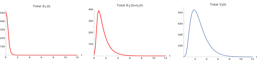
Figure 1: With the advection term $\displaystyle{\vec{C}}={\vec{\bf 0}}$, the population of infected sheep and the population of infected midges are effectively $\displaystyle 0$ at time $\displaystyle t=12$.

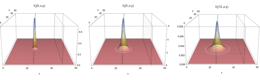
Figure 2: With the advection term $\displaystyle{\vec{C}}={\vec{\bf 0}}$, the short-range movement of midges due to diffusion, is insufficient for the population of infected midges to arrive at $\displaystyle\Omega_{2}$ (centered at $\displaystyle 50\,km$) or $\displaystyle\Omega_{3}$ (centered at $\displaystyle 125\,km$) before time $\displaystyle t=12$. Thus, the epidemic does not break out in $\displaystyle\Omega_{2}$ or $\displaystyle\Omega_{3}$.

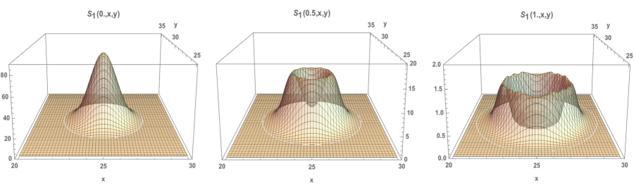
Figure 3: The spatial distributions of the host population $\displaystyle S_{1}(x,y,t)$ at times $\displaystyle t=0.0,\,0.5$, and $\displaystyle 1.0$ with the advection term $\displaystyle{\vec{C}}={\vec{\bf 0}}$. In the absence of long-range movement of midges due to advection, all hosts in $\displaystyle\Omega_{1}$ become infected by time $\displaystyle t=2.0$.

4.1 First simulation - lower advection coefficient

In the first simulation, with the value of $\displaystyle{\vec{C}}=-10.0\left[\begin{array}[]{cc}1\\ 0\\ \end{array}\right]$, the wind-aided long-range movement of BTV infected midges due to advection, plus the short-range movement due to diffusion, is sufficient to transport the infected midges to $\displaystyle\Omega_{2}$. (Figures 4,5, and 6).

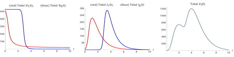
Figure 4: The total populations $\displaystyle S_{1}(t)$, $\displaystyle S_{2}(t)$, $\displaystyle I_{1}(t)$, $\displaystyle I_{2}(t)$, and $\displaystyle V_{I}(t)$ over 10 months. The epidemic breaks out in $\displaystyle\Omega_{2}$ at approximately 2 months. Not all hosts in the 1st site become infected. All hosts in the second site $\displaystyle\Omega_{2}$ become infected by approximately 8 months.

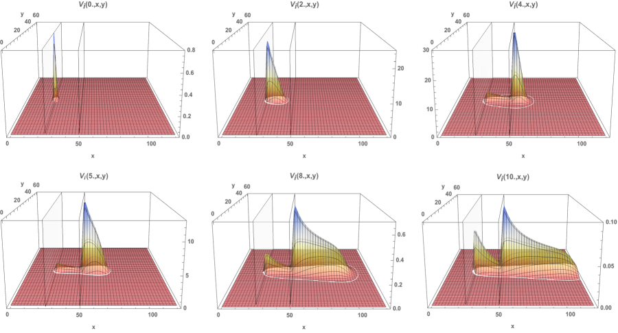
Figure 5: The spatial distributions of the infected vectors $\displaystyle V_{i}(x,y,t)$ at times $\displaystyle t=0,2,4,5,6,10$ months. The long-range wind-aided advection movement plus the short-range diffusion movement of the infected vectors from the first site $\displaystyle\Omega_{1}$ is sufficient to initiate an epidemic outbreak at the second site $\displaystyle\Omega_{2}$ within approximately 2 months.

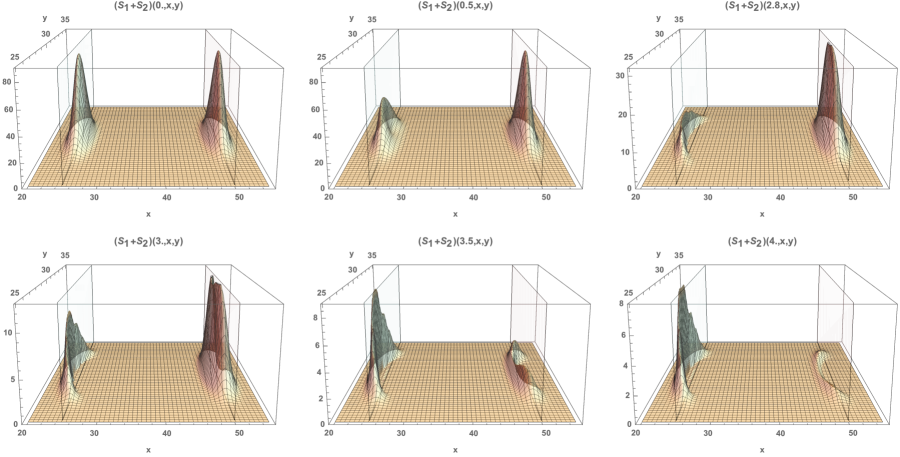
Figure 6: The spatial distributions of the host populations $\displaystyle S_{j}(x,y,t),\,j=1,2$ at times $\displaystyle t=0,0.5,2.8,3,3.5,4$ months.

4.2 Second simulation - higher advection coefficient

In the second simulation, with the value of $\displaystyle{\vec{C}}=-20.0\left[\begin{array}[]{cc}1\\ 0\\ \end{array}\right]$, the wind-aided long-range movement of BTV infected midges due to advection, plus the short-range movement due to diffusion, is sufficient to transport the infected midges to $\displaystyle\Omega_{3}$. (Figures 7, 8, and 9).

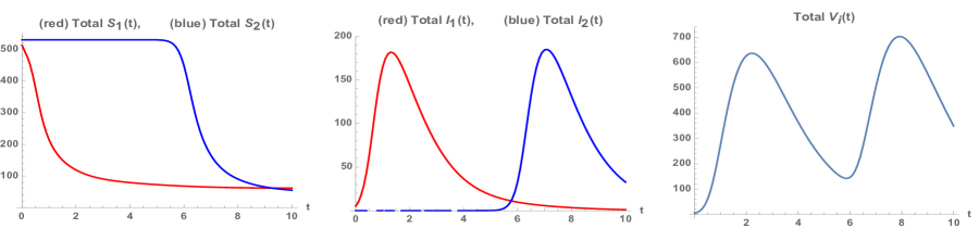
Figure 7: The total populations $\displaystyle S_{1}(t)$, $\displaystyle S_{2}(t)$, $\displaystyle I_{1}(t)$, $\displaystyle I_{2}(t)$, and $\displaystyle V_{I}(t)$ over 10 months. The epidemic breaks out in $\displaystyle\Omega_{2}$ at approximately 5 months. Not all hosts in the 1st site become infected and not all hosts in the second site $\displaystyle\Omega_{2}$ become infected.

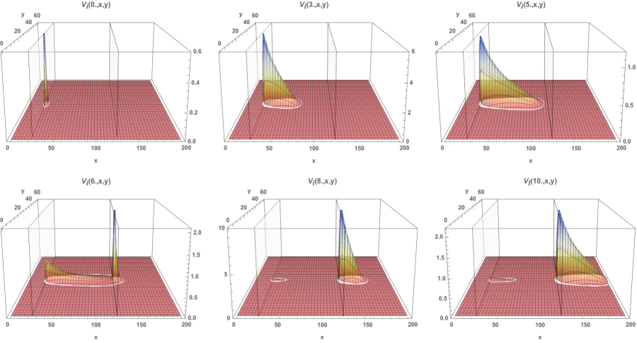
Figure 8: The spatial distributions of the infected vectors $\displaystyle V_{i}(x,y,t)$ at times $\displaystyle t=0,3,5,6,8,10$ months. The long-range wind-aided advection movement plus the short-range diffusion movement of the infected vectors from the first site $\displaystyle\Omega_{1}$ is sufficient to initiate an epidemic outbreak at the second site $\displaystyle\Omega_{3}$ within approximately 5 months.

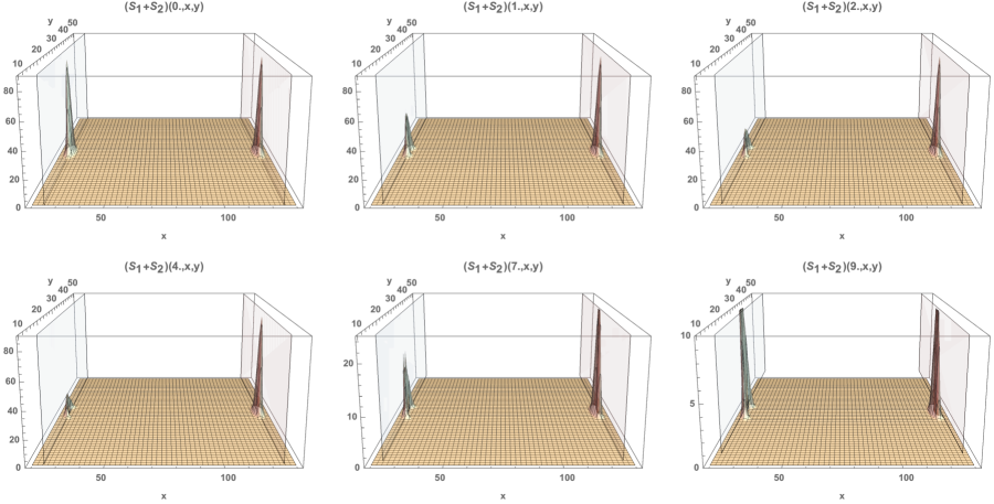
Figure 9: The spatial distributions of the host populations $\displaystyle S_{j}(x,y,t),\,j=1,2$ at times $\displaystyle t=0,1,2,4,7,9$ months.

5 Conclusions and Discussion

We have investigated a spatial vector-host epidemic model, with hosts confined to small non-overlapping domains, and vectors moving throughout a much larger domain. The motivation of our model is to understand how an epidemic outbreak in one small region can transport to outbreaks in distant regions, in the absence of contact between hosts in these widely separately regions. The spatial movement of vectors is modeled by diffusion terms and advection terms in the model equations. The diffusion terms correspond to general short-range spatial movement and the advection terms corresponds to long-range spatial movement in a specified direction.

We have analyzed the dynamics of the model and characterized the behavior of solutions over time. Numerical simulations illustrate how the bluetongue disease can spread from one sheep heart to other geographically separated herds . In these simulations the transport of the disease from an outbreak location to a distant location is dependent upon the magnitude of the advection term. The interpretation of the advection term is wind-aided movement of infected midges, which can be carried to distant uninfected sheep, if the wind-aided movement is sufficiently strong, but not so strong that it disperses the infected midges to values too low at out-lying sites. Our simulations have illustrated our model with three host subregions. In reality, there are a very large number of subregions in a much larger region of inhabitation of the midge population. These multiple subregions allow successive subregion-to-subregion inter-transport of infected midges by long-range movement, as represented by the simulations with only two subregions.

Our model is a simplified formulation of the biological processes in many respects. The model is formulated as a system of continuum partial differential equations, which relate parameter values of the model equations over time. These parameters capture average values of the dynamical processes, with possibly wide ranges of values represented by these averages, The reality of the epidemic processes is extremely complex, and is dependent on an extreme variation in the dynamical processes. Our simplified models, however, capture the essential elements of this class of host-vector epidemics, and provide insight into essential epidemiological behavior.

References

• [1] E.C. Agren, L. Burgin, L.S. Sternberg, K. Gloster, and M. Elvander, Possible means of introduction of bluetongue virus serotype 8 (BTV-8) to Sweden in August 2008: comparison of results from two models for atmospheric transport of the Culicoides vector, Vet. Record., 167(2010), 484-488.
• [2] A. Alba, J. Casal, and M. Domingo, Possible introduction of bluetongue into the Balearic Islands, Spain, via air streams, Vet. Record., 155 (2004), 460-431.
• [3] L.J.S. Allen, B.M. Bolker, Y. Lou, and A.L. Nevai, Asymptotic profiles of the steady states for an SIS epidemic reaction-diffusion model, Discrete and Continuous Dynamical Systems, 21(1) (2008), 1-20.
• [4] H. Amann, Quasi-linear evolution equations and parabolic systems, Transactions of the American Mathematical Society (1986), 197-227.
• [5] S. Anita, W.E. Fitzgibbon, and M. Langlais, Global existence and internal stabilization for a reaction-diffusion system posed on noncoincident spatial domains, Discrete and Continuous Dynamical Systems-Series B, 11(4) (2009), 805-822.
• [6] Y. Braverman, and F. Chechik, Air streams and the introduction of animal diseases borne on Culicoides (Diptera, Ceratopogonidae) into Israel. Revue scientifique et technique (International Office of Epizootics), 15(3) (1996): 1037-1052.
• [7] R.J. Brenner, M.J. Wargo, G.S. Staines, and M.S. Mulla, The dispersal of Culicoides mohave (Diptera: Ceratopogonidae) in the desert of southern California, Mosq. News, 44 (1984), 343-350.
• [8] L.E. Burgin, J. Gloster, C. Sanders, P.S. Mellor, S. Gubbins, and S. Carpenter, Investigating incursions of bluetongue virus using a model of long?distance Culicoides biting midge dispersal, Transboundary and emerging diseases, 60(3) (2013): 263-272.
• [9] R.S. Cantrell and C. Cosner, Spatial Ecology Via Reaction-diffusion Equations, John Wiley & Sons, 1981.
• [10] V. Capasso, Global solution for a diffusive nonlinear deterministic epidemic model, SIAM Journal on Applied Mathematics, 35(2) (1978), 274-284.
• [11] S. Carpenter, M.H. Groschup, C. Garros, M.L. Felippe-Bauer, and B.V.Purse, Culicoides biting midges, arboviruses and public health in Europe, Antiviral Res., 100(1) (2013), 102-113.
• [12] A.C. CuΓ©llar, et al., Spatial and temporal variation in the abundance of Culicoides biting midges (Diptera: Ceratopogonidae) in nine European countries, Parasites $\displaystyle\&$ Vectors, 11:112 (2018).
• [13] M.V.P. Charron, H. Seegers, M. Langlais, and P. Ezanno, Seasonal spread and control of bluetongue in cattle, J. Theoret. Biol., 291(2011), 1-9
• [14] M.V.P. Charron, G. Kluiters, M. Langlais, H. Seegers, M. Baylis, and P. Ezanno, Seasonal and spatial heterogeneities in host and vector abundances impact the spatiotemporal spread of bluetongue, Vet. Res., 44 (2014), 44.
• [15] E. Ducheyne, R. De Deken, S. B cu, B. Codina, K. Nomikou, O. Mangana-Vougiaki, G. Georgiev, B.V. Purse, and G. Hendrickx, Quantifying the wind dispersal of Culicoides species in Greece and Bulgaria, Geospatial Health, 1(2) (2007): 177-189.
• [16] E. FernΓ‘ndez-CarriΓ³n, B. Ivorra , A.M. Ramos, B. MartΓ­nez-LΓ³pez, C. Aguilar-Vega, and J. M. SΓ‘nchez-VizcΓ‘ no, An advection-deposition-survival model to assess the risk of introduction of vector-borne diseases through the wind: Application to bluetongue outbreaks in Spain, PLOS ONE, (2018), March 22.
• [17] R.A. Fisher, The wave of advance of advantageous genes, Annals of eugenics, 7 (1937): 355-369.
• [18] W.E. Fitzgibbon, C.B. Martin, and J.J. Morgan, A diffusive epidemic model with criss-cross dynamics, Journal of Mathematical Analysis and Applications, 184(3) (1994), 399-414.
• [19] W.E. Fitzgibbon, M.E. Parrott, and G.F. Webb, Diffusion epidemic models with incubation and crisscross dynamics, Mathematical Biosciences, 128(1) (1995), 131-155.
• [20] W.E. Fitzgibbon, M.E. Parrott, and G.F. Webb, A diffusive age-structured SEIRS epidemic model, Methods and Applications of Analysis, 3 (1996), 358-369.
• [21] W.E. Fitzgibbon, M. Langlais, and J.J. Morgan, A reaction-diffusion system modeling the direct and indirect transmission of diseases, Discrete and Continuous Dynamical Systems, Series B, 4 (2004), 893-910.
• [22] W.E. Fitzgibbon, M. Langlais, and J.J. Morgan, A reaction-diffusion system on noncoincident spatial domains modeling the circulation of a disease between two host populations, Differential and integral equations, 17(7-8) (2004), 781-802.
• [23] W.E. Fitzgibbon, M. Langlais, F. Marpeau, and J.J. Morgan, Modeling the circulation of a disease between two host populations on noncoincident spatial domains, Biological Invasions, 7(5) (2005), 863-875.
• [24] W.E. Fitzgibbon, M.E. Parrott, and G.F. Webb, Diffusive epidemic models with spatial and age dependent heterogeneity, Discrete and Continuous Dynamical Systems, 1 (2005), 35-57.
• [25] W.E. Fitzgibbon, and M. Langlais, Simple models for the transmission of microparasites between host populations living on noncoincident spatial domains, Structured Population Models in Biology and Epidemiology, Springer , New York, 2008, 115-164.
• [26] W.Β E. Fitzgibbon, J.Β J. Morgan, and G.Β F. Webb. An outbreak vector-host epidemic model with spatial structure: the 2015-2016 zika outbreak in rio de janerio. Theoretical Biology and Medical Modelling, 14:7 (2017).
• [27] W.E. Fitzgibbon, J.J. Morgan, G.F. Webb, Y. Wu, A vector?host epidemic model with spatial structure and age of infection, Nonlinear Analysis: Real World Applications, 41 (2018), 692-705.
• [28] S.A. Gourley, G. RΓΆst, and H.R. Thieme, Uniform persistence in a model for bluetongue dynamics, SIAM J. Math. Anal., 46:2 (2014), 1160-1184.
• [29] K. Graesboll, T. Sumner, C. Enoe, L.E. Christiansen, and S. Gubbins, A comparison of dynamics in two models for the spread of a vector-borne disease, Transbound. Emerg. Dis., 63(2) (2014), 215-223.
• [30] S. Gubbins, S. Carpenter, M. Baylis, J.L Wood, and P.S. Mellor, Assessing the risk of bluetongue to UK livestock: uncertainty and sensitivity analyses of a temperature-dependent model for the basic reproduction number, J. Roy. Soc. Interface, 5 (2008), 363-371.
• [31] H.Guis, C. Caminade, C. Calvete, A.P. Morse, A. Tran, and M. Baylis, Modelling the effects of past and future climate on the risk of bluetongue emergence in Europe, J. Roy. Soc. Interface, 9 (2012), 339-350.
• [32] G. Hendfickx, M. Gilbert, C. Staubach, A. Elbers, K. Mintiens, G. Gerber, and E. Ducheyne, A wind density model to quantify the airborne spread of Culicoides species during north-western Europe bluetongue epidemic, 2006, Prev. Vet. Med., 87 (2008), 162-181.
• [33] C. Johansen, et al. Wind-borne mosquitoes: Could they be a mechanism of incursion of Japanese encephalitis virus into Australia? 4th Mosquito Control Assn of Australia Symposium 8 (2001), 180-185.
• [34] J.K. Kelso and G.J. Milne, A spatial simulation model for the dispersal of thebluetongue vector Culicoides brevitarsis in Australia, PLOS ONE, 9(8) (2014).
• [35] N.J. Maclachlan, Bluetongue: history global epidemiology and pathogenesis, Prevent. Vet. Med., 102 (2011), 107-111.
• [36] L. McDill, Bluetongue virus, in Newsletter, Indiana Animal Disease Laboratory, Purdue University, West Lafayette, Indiana Spring 2002, https://www.addl.purdue.edu/newsletters/2002/spring/bluetongue.shtml.
• [37] P.S. Mellor, J. Boorman, and M. Baylis, Culicoides biting midges: their role as arbovirus vectors. Annu. Rev. Entomol. bf 45 (2000), 307-340.
• [38] M.D. Murray, Akabane epizootics in New South Wales: evidence for long?distance dispersal of the biting midge Culicoides brevitarsis, Australian Veterinary, 64(10) (1987), 305-308.
• [39] M. Pioz, H. Guis, D.B. Calavas, D. Abrial, and C. Ducrot, Estimating front-wave velocity of infectious diseases: a simple, efficient method applied to bluetongue. Vet. Res. 42 (2011), 60.
• [40] B. V. Purse, V. Bethan., P.S. Mellor, S. Philip, D.J. Rogers, A.R. Samuel, P. Mertens, and M. Baylis, Climate change and the recent emergence of bluetongue in Europe, Nat. Rev. Microb., 3 (2) (2005), 171-181.
• [41] B.V. Purse, S. Carpenter, G.J. Venter, G. Bellis, and B.A. Mullens, Bionomics of temperate and tropical Culicoides midges: knowledge gaps and consequences for transmission of Culicoides-borne viruses, Annu. Rev. Entomol., 60 (2015), 373-392.
• [42] A. Ssematimba, T.J. Hagenaars, and M.C. De Jong, Modelling the wind-borne spread of highly pathogenic avian influenza virus between farms, PLoS One, 7(2)(2012): p.e31114.
• [43] L. Sedda, H.E. Brown, B.V. Purse, L. Burgin, J. Gloster, and D.J. Rogers, A new algorithm quantifies the roles of wind and midge flight activity in the bluetongue epizootic in northwest Europe, Proc. R. Soc. B, 279 (2012), 2354-2362.
• [44] R.F. Sellers, D.E. Pedgley, and M.R. Tucker, Possible windborne spread of bluetongue to Portugal, June-July 1956. J. Hygiene 81 (1978), 189-196.
• [45] R.F. Sellers, E.P. Gibbs, K.A. Herniman, D.E. Pedgley, and M.R. Tucker, Possible origin of the bluetongue epidemic in Cyprus, August 1977, J. Hygiene, 83 (1979), 547-555
• [46] J. Smoller, Shock waves and reaction-diffusion equation, Springer-Verlag, New-York, 1984.
• [47] T. Sumner, R.J. Orton, D.M. Green, R. R. Kao, and S. Gubbins, Quantifying the roles of host movement and vector dispersal in the transmission of vector-borne diseases of livestock, PloS Comp. Biol, 13-4 (2017).
• [48] G.F. Webb, A reaction-diffusion model for a deterministic diffusive epidemic, Journal of Mathematical Analysis and Applications, 84(1) (1981), 150-161.
• [49] S.M. White, C.J. Sanders, C.R. Shortall, and B.V. Purse, Mechanistic model for predicting the seasonal abundance of Culicoides biting midges and the impacts of insecticide control, Parasites $\displaystyle\&$ Vectors 10:162 (2017).
• [50] Wikipedia, Bluetongue Disease, www.wikipedia.org/wiki/Bluetongue-disease.
• [51] A. Wilson, K. Darpel, and P.S. Mellor, Where does bluetongue virus sleep in the winter, PLoS Biol., 6(80) (2008).