Thermodynamics and phase transitions of galactic clustering in higher-order Modified Gravity

Abstract

We study the thermodynamics of galactic clustering under the higher-order corrected Newtonian dynamics. The clustering of galaxies is considered as a gravitational phase transition. In order to study the effects of higher-order correction to the thermodynamics of gravitational system, we compute more exact equations of state. Moreover, we investigate the corrected probability distribution function for such gravitating system. A relation between order parameter and the critical temperature is also established.

Keywords: Modified gravity; Thermodynamics; Large scale structure; Distribution function.

PACS Numbers: 95.30.Sf ; 05.70.-a.

I Overview and Motivation

Because of gravitational interaction of galaxies, the characterization of galactic clustering is a subject of extensive interest. It is well known that the gravitational interaction between clusters of galaxies plays an important role in the evolution of universe. A mathematical description which explains the current behavior of universe and its evolution over time is known as the cosmological model. The considered cosmological model in this paper is based on the fundamental assumptions which may explain numerous observations. Though it is clear that there is some missing mass in the universe which is known as the dark matter. This is because of the gravitational effects on the clusters of galaxies. There are some reports available on expected discoveries of dark matter ber , while direct observation for the dark matter does not exist. Dark matter doesn’t interact electromagnetically which make it impossible to detect. A less explored route is that our current theory explaining universe might be incomplete. Milgrom has proposed an empirically motivated modification of Newtonian dynamics at low accelerations, known as MOND mil , which has been found extremely successful in explaining some observational properties of galaxies san22 . Yang et. al. shows how modification of the Newtonian potential would modify the gravitational effects on the statistical mechanics yang and it was the first analysis of clustering with modifications of Newtonian gravity. Also, if the MOND approach is not covariant and hence cannot be studied in a general setting, it is possible to show that this can be framed in the weak field limit of $f(R)$ gravity bernal . A relativistic MOND theory is explored which resolves the problems of gravitational lensing, violated hallowed principles by exhibiting superluminal scalar waves or an a priori vector field beke . MOND also predicts the detailed shape of a rotation curve from the observed matter distribution successfully kent ; milo ; beg . In fact, many theoretical model and indirect study are devoted to understanding the nature of the dark matter ell ; mc ; by ; hassan1 . Also, there are some unified theories of the dark universe including dark energy and dark matter uni3 ; uni4 ; uni5 ; uni6 ; uni1 ; uni2 .

The idea of modifying gravity on cosmological scales has been interesting over the past decade. In this context, recently in the weak field limit of $f(R)$ gravity, it is shown that the corrected gravitational potential allows estimating the total mass of a sample of 12 clusters of galaxies and provides a fair fit to the mass of visible matter estimated by X-ray observations cap . It has been discussed that the Newtonian potential modified at large distances due to the gravity propagation into the bulk flo . The corrections in Newtonian potential are also parametrized by Yukawa potential long ; annalen ; salzano . The idea of modified gravity has been re-emerging with various justifications, see for example Refs. ec ; ha ; dr ; rep1 ; rep2 . The MOND is also studied for the Milky Way and has found that inner Milky Way is completely dominated by baryon matter, which is in agreement with the predictions of standard cold dark matter (CDM) cosmology bb . The good fits of MOND are found in 15 rotation curves of low surface brightness galaxies wj . In the context of MOND, the growth of inhomogeneities in a low-density is presented in the Ref. san1 . On the same track, there are fits of samples of galaxies (mainly low surface brightness) whose dynamics are addressed without dark matter while adopting the $f(R)$ approach cardone ; salucci . There are semi-analytical models for the disk galaxies formation in the universe dominated by dark matter, and also for the cases where the force law is given by modified Newtonian dynamics (MOND) fca . It may be interesting to note that these models are tuned to fit the observed near-infrared Tully-Fisher relation fca .

On the other hand, phase transitions are the fundamental property of interacting systems which has an important role. From the statistical mechanics point of view, there is a connection between the macroscopic phases and the microscopic properties of the given system. If there are different states in the separate regions of multi-dimensional phase space, the transition is called first-order. However, other transitions, where states are close to each other in the phase space, are called second-order. The effects of higher-order corrections on the phase transition of the clustering of particles interacting through Newton’s law have been studied in Ref. sas2 . Recently, the various characterization of clustering of galaxies under the modified gravity are studied st ; san ; mils ; sud ; mir ; MNRAS-Pour ; PRD-Sud ; MNRAS-Sud ; Dark-Sud . For instance, a test using gas rich galaxies for which both axes of the baryonic Tully-Fisher relation can be measured independently of the theories have been done without the systematic uncertainty in stellar mass st . The effect of dark energy on the galactic clustering under the modified Newton’s law by cosmological constant is studied recently sud . A brane world modified Newton’s gravity in the context of galaxy clustering is also analysed mir . The motivation of this paper is to extend the work of Saslaw and Ahmad sas2 by means of modified Newton’s dynamics.

The zeroth-order thermodynamics of galactic clustering in the context of dark energy modification MNRAS-Pour , and a particular modification of gravity PRD-Sud ; MNRAS-Sud ; Dark-Sud have been studied already. As the second and higher-order corrections to thermodynamics of galaxy clustering could become important near phase transitions as clustering increases, so we want to analyse this. Now, we would like to study the higher-order correction to the thermodynamics of system of galaxies under modified gravity. In this work, we study the higher-order correction to the partition function for the gravitating system under the modified Newton’s law. In order to study the thermodynamics of galactic system, first of all we derive the higher-order corrected partition function. With the help resulting partition function, we demonstrate the Helmholtz free energy, entropy, pressure, internal energy and the chemical potential of the system. We find that these thermodynamical quantities include corrections due to higher-order term. A comparison with the standard expressions of the equations of state leads to the higher-order corrected clustering parameter, which characterizes the higher-order effects on the clustering of galaxies under modified gravity. We discuss both the cases of the point mass and the extended mass structures of the galaxies. The study of extended mass structured galaxies through string theory or theory of infinitely extended particles Hes1 ; Hes2 ; Hes3 is interesting. Under assumption that system follows quasi-equilibrium state, we obtain a higher-order corrected distribution function for the system of galaxies. If the higher-order correction parameter is turned-off, we get the lowest-order distribution function of the system interacting through modified gravity. In order to study the phase transition of clusters of galaxies, it is important to investigate the order parameter. Here we found that the clustering parameter as an order parameter under the modified gravity behaves very similar to the pure Newtonian gravity case. We find that under modified Newton’s law, the specific heat for completely virialized system becomes negative as bound clusters dominate. Further, the order parameter, pressure and internal energy are formulated in terms of critical temperature. These results are very general which are valid for any kind of the modified gravity as our computations are based on the general modified gravity.

The presentation of the paper is as follows. In section II, we discuss the higher-order expansion of two-particle function in modified Newtonian gravity and obtain the higher-order corrected partition function. In section III, we evaluate the more exact equation of states corresponding to these higher-order corrections. The expression for clustering parameter is obtained, which describes the distribution of galaxies cluster. In the subsequent section, we invoke the corrected distribution function which exhibits the correction and agrees with the data. In section V, we discuss the role of clustering parameter as order parameter under the modified gravity circumstances. The critical temperature, which maximizes specific heat, is evaluated in section VI. Final discussion with the future remarks is reported in the last section.

II Higher-order corrections to a modified gravity

In this section, we study the higher-order corrected partition function by considering the gravitational system interacting under the modified Newton’s gravity.

II.1 Thermodynamic equations

Our analysis is based on the important assumption that the clustering of the galaxies (as gravitating particles) in the expanding universe evolve in the quasi-equilibrium manner, which is a consequence of equilibrium states, and thus forms an ensemble of comoving cells. For such a large system, the all cells of the ensemble are of the equal volume $V$ and equal average density. According to the standard classical statistical mechanics, the partition function of a system of $N$ particles (galaxies) of mass $m$, interacting with a gravitational potential energy $\Phi$, and average temperature $T$ is given by ahm02 :

$$Z_{N}(T,V)=\frac{1}{N!}\left(\frac{2\pi mT}{\lambda^{2}}\right)^{3N/2}Q_{N}(T,V),$$ (1)

where the configurational integral, $Q_{N}(T,V)$, in terms of two-particle function $f_{ij}$ can be expressed as:

$$Q_{N}(T,V)=\int....\int\biggl{[}(1+f_{12})(1+f_{13})(1+f_{23})(1+f_{14})\dots(1+f_{N-1,N})\biggr{]}d^{3}r_{1}d^{3}r_{2}\dots d^{3}r_{N}.$$ (2)

The two-particle function and gravitational potential energy have following relation:

$$f_{ij}=e^{-\Phi(r_{ij})/T}-1.$$ (3)

We note that the two-particle function exists only if interactions are present there in the system.

We are interested in modified Newtonian gravity here because MOND paradigm can boast of some successful predictions regarding galactic dynamics. The departure of gravitation from Newtonian theory due to MOND should be inside the virial radius, where dynamical accelerations are negligibly small from the perspective to MOND. The gravitational potential modified by a sufficiently regular function ${\mathcal{F}}(r_{ij})$ san is given by

$$\Phi(r_{ij})=-\frac{Gm^{2}}{\sqrt{r_{ij}^{2}+\epsilon^{2}}}-{\mathcal{F}}(r_{ij},\epsilon),$$ (4)

where a softening parameter $\epsilon$ is used to take care of divergences caused in Hamiltonian. Also, force ${\mathcal{F}}(r_{ij},\epsilon)$ is infinitesimal at large distance. By exploiting Eqs. (3) and (4), the two-particle function can be expressed as following:

$$f_{ij}=\exp\left[\frac{Gm^{2}}{T\sqrt{r_{ij}^{2}+\epsilon^{2}}}+\frac{{\mathcal{F}}(r_{ij},\epsilon)}{T}\right]-1.$$ (5)

By expanding exponential term, this further simplifies to

$$f_{ij}=\left(\frac{Gm^{2}}{T\sqrt{r_{ij}^{2}+\epsilon^{2}}}+\frac{{\mathcal{F}}(r_{ij},\epsilon)}{T}\right)+\frac{1}{2!}\left(\frac{Gm^{2}}{T\sqrt{r_{ij}^{2}+\epsilon^{2}}}+\frac{{\mathcal{F}}(r_{ij},\epsilon)}{T}\right)^{2}+....$$ (6)

Following the standard technique, we evaluate the the configuration integral (2) for above two-particle function over a spherical volume of radius $R_{1}$ for $N=1$ as follows,

$$Q_{1}(T,V)=V.$$ (7)

For $N=2$, the configuration integral $Q_{2}(T,V)$ has the following expression:

$$Q_{2}(T,V)=4\pi V\int_{0}^{R}\left[1+\frac{Gm^{2}}{T\sqrt{r^{2}+\epsilon^{2}}}+\frac{{\mathcal{F}}(r,\epsilon)}{T}+\frac{1}{2!}\left(\frac{Gm^{2}}{T\sqrt{r^{2}+\epsilon^{2}}}+\frac{{\mathcal{F}}(r,\epsilon)}{T}\right)^{2}\right]r^{2}dr.$$ (8)

This further simplifies to,

$$Q_{2}(T,V) = V^{2}\left[1+\frac{3}{2}\frac{Gm^{2}}{RT}\left(\sqrt{1+\frac{\epsilon^{2}}{R^{2}}}+\frac{\epsilon^{2}}{R^{2}}\log\frac{\epsilon/R}{\left[1+\sqrt{1+\frac{\epsilon^{2}}{R^{2}}}\right]}+\frac{2}{Gm^{2}R^{2}}\int_{0}^{R}{\mathcal{F}}(r,\epsilon)r^{2}dr\right)\right.$$ (9)

$$+ \left.\frac{3}{2}\left(\frac{Gm^{2}}{RT}\right)^{2}\left[1-\frac{\epsilon}{R}\tan^{-1}\left(\frac{R}{\epsilon}\right)+\frac{2}{3}\frac{R^{2}}{Gm^{2}}\int_{0}^{R}\frac{{\mathcal{F}}(r,\epsilon)}{\sqrt{r^{2}+\epsilon^{2}}}r^{2}dr\right.\right.$$

$$+ \left.\left.\frac{1}{3}\left(\frac{R}{Gm^{2}}\right)^{2}\int_{0}^{R}{\mathcal{F}}^{2}(r,\epsilon)r^{2}dr\right]\right].$$

We rewrite the equation (9) as follows,

$$Q_{2}(T,V)=V^{2}\big{(}1+\alpha_{1}x+\alpha_{2}x^{2}\big{)},$$ (10)

where the following definitions for dimensionless parameters have been utilized:

$$\alpha_{1}=\sqrt{1+\frac{\epsilon^{2}}{R^{2}}}+\frac{\epsilon^{2}}{R^{2}}\log\frac{\epsilon/R}{\left[1+\sqrt{1+\frac{\epsilon^{2}}{R^{2}}}\right]}+\frac{2}{Gm^{2}R^{2}}\int_{0}^{R}{\mathcal{F}}(r,\epsilon)r^{2}dr,$$ (11)

$$\alpha_{2}=\frac{2}{3}\left[1-\frac{\epsilon}{R}\tan^{-1}\left(\frac{R}{\epsilon}\right)+\frac{2}{3}\frac{R^{2}}{Gm^{2}}\int_{0}^{R}\frac{{\mathcal{F}}(r,\epsilon)}{\sqrt{r^{2}+\epsilon^{2}}}r^{2}dr+\frac{1}{3}\left(\frac{R}{Gm^{2}}\right)^{2}\int_{0}^{R}{\mathcal{F}}^{2}(r,\epsilon)r^{2}dr\right],$$ (12)

$$x=\frac{3}{2}\left(\frac{Gm^{2}}{RT}\right)^{3}=\frac{3}{2}\left(\frac{Gm^{2}}{T}\right)^{3}\rho.$$ (13)

The last definition utilizes the scale transformations $\rho\rightarrow\lambda^{-3}\rho,T\rightarrow\lambda^{-1}T$ and $R\rightarrow\lambda R$, to transform $\frac{Gm^{2}}{RT}\rightarrow(\frac{Gm^{2}}{RT})^{3}$ and $R_{1}\sim\rho^{-1/3}\sim(\bar{N}/V)^{-1/3}$.

In case of point mass galaxies, the dimensionless parameters (11) and (12) reduce to

$$\alpha_{1}|_{\epsilon=0}=1+\frac{2}{Gm^{2}R^{2}}\int_{0}^{R}{\mathcal{F}}(r,0)r^{2}dr,$$ (14)

$$\alpha_{2}|_{\epsilon=0}=\frac{2}{3}\left[1+\frac{2}{3}\frac{R^{2}}{Gm^{2}}\int_{0}^{R}{{\mathcal{F}}(r,0)}rdr+\frac{1}{3}\left(\frac{R}{Gm^{2}}\right)^{2}\int_{0}^{R}{\mathcal{F}}^{2}(r,0)r^{2}dr\right].$$ (15)

The configuration integral for $N$ particles case can be obtained recursively as following:

$$Q_{N}(T,V)=V^{N}\big{(}1+\alpha_{1}x+\alpha_{2}x^{2}\big{)}^{N-1}.$$ (16)

Plugging this resulting $N$ particles configuration integral in to (1), we obtain the explicit expression of gravitational partition function as

$$Z_{N}(T,V)=\frac{1}{N!}\left(\frac{2\pi mT}{\lambda^{2}}\right)^{3N/2}V^{N}\big{(}1+\alpha_{1}x+\alpha_{2}x^{2}\big{)}^{N-1}.$$ (17)

This is the higher-order corrected partition function of $N$ particles (galaxies) interacting under modified Newtonian potential.

III Equations of State

The gravitational system (galaxies cluster) can be described adequately by macroscopic thermodynamic variables, such as total energy ($U$), Helmholtz free energy ($F$), Gibbs free energy ($G$), enthalpy ($H$) entropy ($S$), temperature ($T$), pressure ($P$), volume ($V$), number of particles (galaxies) ($N$) and chemical potential ($\mu$). We compute these thermodynamic quantities for the infinite statistically homogeneous system of gravitating particles which are characterized by exact equations of state. As we have expression for the gravitational partition function (17), these thermodynamic quantities can be easily calculated. For instance, utilizing relation $F=-T\ln Z_{N}(T,V)$, the Helmholtz free energy is demonstrated as

$$F=-T\ln\biggl{[}\frac{1}{N!}\left(\frac{2\pi mT}{\lambda^{2}}\right)^{3N/2}V^{N}\big{(}1+\alpha_{1}x+\alpha_{2}x^{2}\big{)}^{N-1}\biggr{]}.$$ (18)

The Helmholtz free energy is nothing but the thermodynamic potential that measures the work obtainable from a thermodynamic system at a constant temperature. The negative of the difference in the Helmholtz energy gives information regarding the maximum amount of work that the system can perform in a thermodynamic process in which volume is held constant. Further simplification leads to,

$$F=NT\ln\left(\frac{N}{V}T^{-3/2}\right)-NT-(N-1)T\ln\big{(}1+\alpha_{1}x+\alpha_{2}x^{2}\big{)}-\frac{3}{2}NT\ln\left(\frac{2\pi m}{\lambda^{2}}\right).$$ (19)

Although $\alpha_{1}$ and $\alpha_{2}$ depend on ${{\mathcal{F}}(r,\epsilon)}$, but can be fix as they are independent of $N$, $V$ and $T$. In that case, we can obtain graphical behavior of the Helmholtz free energy by varying $\alpha_{1}$ and $\alpha_{2}$. In the Fig. 1, we can see the behavior of Helmholtz free energy with respect to $N$. We can see a minimum which is corresponding to the maximum of distribution function calculated later. There exists critical $N$ also where Helmholtz free energy vanishes, which means that the cluster of galaxies is at equilibrium. For large $N$, we can see a divergence in the Helmholtz free energy which yields to the state out of equilibrium. The last line, which is drawn for $\alpha_{1}>0$ and $\alpha_{2}>0$, may correspond to the case of ${{\mathcal{F}}(r,\epsilon)}=0$. It means that the effect of higher-order correction is a decreasing potential.

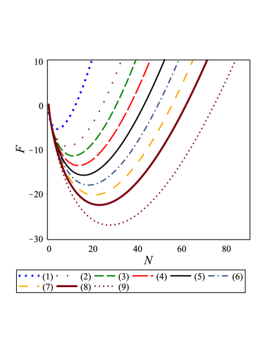
Figure 1: Typical behavior of Helmholtz free energy in terms of particle number with variation of $\alpha_{1}$ and $\alpha_{2}$ and unit value for other parameters. (1) $\alpha_{1}<0$, $\alpha_{2}<0$;   (2) $\alpha_{1}=0$, $\alpha_{2}<0$;   (3) $\alpha_{1}<0$, $\alpha_{2}=0$;   (4) $\alpha_{1}>0$, $\alpha_{2}<0$;   (5) $\alpha_{1}=0$, $\alpha_{2}=0$;   (6) $\alpha_{1}<0$, $\alpha_{2}>0$;   (7) $\alpha_{1}>0$, $\alpha_{2}=0$;   (8) $\alpha_{1}=0$, $\alpha_{2}>0$;   (9) $\alpha_{1}>0$, $\alpha_{2}>0$.

The next step is to derive entropy in terms of the model parameters. The entropy and the free energy are related by following expression: $S=-\biggl{(}\frac{\partial F}{\partial T}\biggr{)}_{N,V}$. Therefore, for a given Helmholtz free energy (19), the entropy reads

$$S=N\ln\left(\frac{V}{N}T^{3/2}\right)+(N-1)\ln\big{(}1+\alpha_{1}x+\alpha_{2}x^{2}\big{)}-3(N-1)\frac{\alpha_{1}x+2\alpha_{2}x^{2}}{1+\alpha_{1}x+\alpha_{2}x^{2}}+\frac{5}{2}N+\frac{3}{2}N\ln\left(\frac{2\pi m}{\lambda^{2}}\right).$$ (20)

For the large $N$, we can use $N-1\approx N$ approximation and, thus, the specific entropy is simplified to

$$\frac{S}{N}=\ln\left(\frac{V}{N}T^{3/2}\right)-\ln\left(1-\frac{\alpha_{1}x+\alpha_{2}x^{2}}{1+\alpha_{1}x+\alpha_{2}x^{2}}\right)-3\frac{\alpha_{1}x+2\alpha_{2}x^{2}}{1+\alpha_{1}x+\alpha_{2}x^{2}}+\frac{S_{0}}{N},$$ (21)

where $S_{0}=\frac{5}{2}N+\frac{3}{2}N\ln\left(\frac{2\pi m}{\lambda^{2}}\right)$ is the fiducial entropy. Here we notice that, for $\alpha_{1}=\alpha_{2}=0$, this reduces to the perfect classical gas case.

The internal energy of a gravitational system is the energy contained within the system, including the kinetic and potential energy as a whole. For given state of a system it cannot be measured directly. However, once you know the state variables of the system, free energy $F$, temperature $T$ and entropy $S$, the internal energy can easily be calculated through relation, $U=F+TS$. This follows,

$$U=\frac{3}{2}NT\left(\frac{1-\alpha_{1}x-3\alpha_{2}x^{2}}{1+\alpha_{1}x+\alpha_{2}x^{2}}\right).$$ (22)

We observe here to, that the perturbation from perfect classical gas is due to non-vanishing parameters till higher-order $\alpha_{1}$ and $\alpha_{2}$.

By the relation $P=-\left(\frac{\partial F}{\partial V}\right)_{N,T}$, it is straightforward to calculate pressure equation of state, which is given by

$$P=\frac{NT}{V}\left(\frac{1-\alpha_{2}x^{2}}{{1+\alpha_{1}x+\alpha_{2}x^{2}}}\right).$$ (23)

Then, by using the relation $G=F+PV$, one can obtain Gibbs free energy which behaves as the Helmholtz free energy. Chemical potential $\mu$ gives information about the change in internal energy if one particle is added to the system, while keeping all other thermodynamic quantities constant. In order to derive chemical potential, we exploit the relation $\mu=\biggl{(}\frac{\partial F}{\partial N}\biggr{)}_{V,T}$ and get

$${\mu}={T}\ln\left(\frac{N}{V}T^{-3/2}\right)-{T}\ln\big{(}1+\alpha_{1}x+\alpha_{2}x^{2}\big{)}-\frac{3}{2}{T}\ln\left(\frac{2\pi m}{\lambda^{2}}\right)-{T}\frac{\alpha_{1}x+2\alpha_{2}x^{2}}{1+\alpha_{1}x+\alpha_{2}x^{2}}.$$ (24)

In the above expression of chemical potential, an extra term of order $x^{2}$ is present which (physically) represents the energy required to put in a galaxy to under-virialized clustering regions and this, of course, will affect the distribution functions. In the Fig. 2, we can see a typical behavior of the chemical potential with $N$ for different values of $\alpha_{1}$ and $\alpha_{2}$. There exist some critical $N$ also where $\mu=0$, which means that $\frac{\partial S}{\partial N}=0$. It is clear that as $N$ increases (decreases) $\mu$ increases (decreases). More precisely, if the number density $\frac{N}{V}$ increases (decreases) with fixed $T$, the chemical potential increases (decreases). The last line, which is dash dot green line, may corresponds to the case of ${{\mathcal{F}}(r,\epsilon)}=0$. It tells us that the higher-order correction is increasing the chemical potentials.

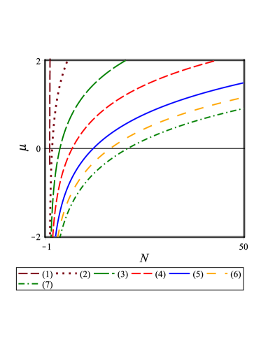
Figure 2: Typical behavior of Chemical potential in terms of particle number with variation of $\alpha_{1}$ and $\alpha_{2}$, we set unit value for other parameters. (1) $\alpha_{1}<0$, $\alpha_{2}<0$;   (2) $\alpha_{1}=0$, $\alpha_{2}<0$;   (3) $\alpha_{1}<0$, $\alpha_{2}=0$;   (4) $\alpha_{1}=0$, $\alpha_{2}=0$;   (5) $\alpha_{1}<0$, $\alpha_{2}>0$;   (6) $\alpha_{1}=0$, $\alpha_{2}>0$;   (7) $\alpha_{1}>0$, $\alpha_{2}>0$.

Equating above expressions of thermodynamic quantities to their standard forms given in terms of clustering parameter (for details see, e.g., ahm02 ), the value of higher-order corrected clustering parameter, $\mathcal{B}$, for the system of galaxies in the expanding universe emerges, naturally, as

$$\mathcal{B}=\frac{\alpha_{1}x+2\alpha_{2}x^{2}}{1+\alpha_{1}x+\alpha_{2}x^{2}}.$$ (25)

It should be noted that the clustering parameter plays an important role in the clustering of galaxies. For the point mass case ( i.e., $\epsilon=0$), the higher-order corrected clustering parameter in modified potential energy takes following value:

$$\mathcal{B}_{0}=\frac{\left[1+\frac{2}{Gm^{2}R^{2}}\int_{0}^{R}{\mathcal{F}}(r,0)r^{2}dr\right]x+\frac{4}{3}\left[1+\frac{2}{3}\frac{R^{2}}{Gm^{2}}\int_{0}^{R}{{\mathcal{F}}(r,0)}rdr+\frac{1}{3}\left(\frac{R}{Gm^{2}}\right)^{2}\int_{0}^{R}{\mathcal{F}}^{2}(r,0)r^{2}dr\right]x^{2}}{1+\left[1+\frac{2}{Gm^{2}R^{2}}\int_{0}^{R}{\mathcal{F}}(r,0)r^{2}dr\right]x+\frac{2}{3}\left[1+\frac{2}{3}\frac{R^{2}}{Gm^{2}}\int_{0}^{R}{{\mathcal{F}}(r,0)}rdr+\frac{1}{3}\left(\frac{R}{Gm^{2}}\right)^{2}\int_{0}^{R}{\mathcal{F}}^{2}(r,0)r^{2}dr\right]x^{2}}.$$ (26)

Here we notice that for Newtonian potential energy, i.e., $\mathcal{F}(r)=0$, the higher-order corrected clustering parameter has the following form:

$$\mathcal{B}_{0}=\frac{x+\frac{4}{3}x^{2}}{1+x+\frac{2}{3}x^{2}}.$$ (27)

This coincides with the original clustering parameter $b=\frac{x}{1+x}$ for galaxies with point mass structure when the higher-order corrections are switched off.

IV Corrected Distribution Function

In order to obtain the higher-order corrected gravitational quasi-equilibrium distribution function $f(N)$, we follow the method discussed in Ref. sas1 . We consider a grand canonical ensemble of cells with the same shape and volume, which are much smaller than the total gravitational system. Here, the number of galaxies and their mutual gravitational energy varies among cells. The probability of finding a particular number of galaxies in a cell of volume $V$ follows from summation over all energy states, i.e.,

$$p(N)=\sum_{i}\Omega_{Ni},$$ (28)

where $\Omega_{N_{i}}$ is the probability of finding $N_{i}$ particles in the energy states $U_{i}(N_{i},V)$ with the following expressions:

$$\Omega_{Ni}=\frac{e^{N_{i}\mu/T-U_{i}/T}}{{Z_{G}(T,V,\mu)}}$$ (29)

Here, the grand canonical partition function has following expression:

$$Z_{G}(T,V,\mu)=\sum_{i}e^{\frac{N_{i}\mu-U_{i}}{T}}=e^{-\frac{\Psi}{T}},$$ (30)

where $\Psi$, so-called the grand canonical potential, is nothing but the Legendre transformation of the average energy concerning both $S$ and $N$. Hence, this can be given by $\Psi=-PV$. Now, by exploiting relation (23), the higher-order corrected grand partition function (30) for the galaxies interacting through modified gravity is calculated by

$$Z_{G}=e^{\frac{PV}{T}}=e^{\bar{N}(1-\mathcal{B})}.$$ (31)

The probability of finding $N$ particles in a cell of volume $V$ is given by

$$p(N,\epsilon)=e^{\frac{N\mu}{T}}\left(\sum_{i}e^{\frac{-U_{i}}{T}}\right)e^{-\bar{N}(1-\mathcal{B})}={e^{\frac{N\mu}{T}}Z_{N}(V,T)}e^{-\bar{N}(1-\mathcal{B})}.$$ (32)

Upon solving the quadratic equation (25) for $x$, we get

$$\alpha_{1}x+\alpha_{2}x^{2}=\frac{\mathcal{B}}{1-\mathcal{B}}-\frac{\mathcal{B}^{2}(2-\mathcal{B})}{(1-\mathcal{B})^{3}}\frac{\alpha_{2}}{\alpha_{1}^{2}}.$$ (33)

Now, with the help of Eqs. (17) and (24) together with (14), the distribution function (32) for extended mass particles (galaxies with halos) is demonstrated as

$$p(N,\epsilon)=\frac{\bar{N}^{N}}{N!}\biggl{(}1+\frac{N}{\bar{N}}\frac{\mathcal{B}}{(1-\mathcal{B})}-\frac{N}{\bar{N}}\frac{\mathcal{B}^{2}(2-\mathcal{B})}{(1-\mathcal{B})^{3}}\frac{\alpha_{2}}{\alpha_{1}^{2}}\biggr{)}^{N-1}\biggl{(}1+\frac{\mathcal{B}}{(1-\mathcal{B})}-\frac{\mathcal{B}^{2}(2-\mathcal{B})}{(1-\mathcal{B})^{3}}\frac{\alpha_{2}}{\alpha_{1}^{2}}\biggr{)}^{-N}e^{-N\mathcal{B}-\bar{N}(1-\mathcal{B})}.$$ (34)

By setting $\epsilon=0$, we can get the gravitational quasi-equilibrium distribution function for galaxies with point mass structures as follows,

$$p(N,0)=\frac{\bar{N}^{N}}{N!}\biggl{(}1+\frac{N}{\bar{N}}\frac{\mathcal{B}_{0}}{(1-\mathcal{B}_{0})}-\frac{N}{\bar{N}}\frac{\mathcal{B}_{0}^{2}(2-\mathcal{B}_{0})}{(1-\mathcal{B}_{0})^{3}}\frac{\alpha_{2}}{\alpha_{1}^{2}}\biggr{)}^{N-1}\biggl{(}1+\frac{\mathcal{B}_{0}}{(1-\mathcal{B}_{0})}-\frac{\mathcal{B}_{0}^{2}(2-\mathcal{B}_{0})}{(1-\mathcal{B}_{0})^{3}}\frac{\alpha_{2}}{\alpha_{1}^{2}}\biggr{)}^{-N}e^{-N\mathcal{B}_{0}-\bar{N}(1-\mathcal{B}_{0})}.$$ (35)

This result matches exactly with the result obtained in Ref. sas2 except with modified clustering parameters. The presence of higher-order correction is obvious here as this expression contains $\alpha_{2}$. For $\alpha_{2}\rightarrow 0$, we can get the lowest order gravitational quasi-equilibrium distribution function with modified gravity. Further, for $\mathcal{F}(r)=0$, this reduces to original result discussed in ahm02 .
From the Fig. 3, we can compare the behavior of distribution function with and without higher-order corrections. Here, it is clear that the presence of higher-order correction increases the value of the distribution function. Also, there exists a critical $N$ which maximizes the probability and corresponds to the minimum of free energies.

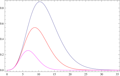
Figure 3: Comparative study of distribution function $p(N,\epsilon)$ (perpendicular axis) versus $N$ (horizontal axis) for extended mass structure for $\mathcal{B}=0.3$, and $\bar{N}=10$. Here, $\alpha_{2}=0$ (Violet bottom line) corresponds to no higher-order corrections, for $\alpha_{2}=2/5,\alpha_{1}=\sqrt{2}$ (Red middle line) and $\alpha_{2}=4/3,\alpha_{1}=\sqrt{2}$ (Magenta top line) denote higher-order corrections.

V Order Parameter for Phase Transition

In order to study the phase transition for galaxies evolution and cluster formation, it is important to analyze the order parameter which characterizes the phase transition. In this regard, let us write the clustering parameter for point mass galaxies under modified potential to lowest order as an order parameter

$$B_{0}=\frac{\left(1+\frac{2}{Gm^{2}R^{2}}\int_{0}^{R}{\mathcal{F}}(r,0)r^{2}dr\right)x}{1+\left(1+\frac{2}{Gm^{2}R^{2}}\int_{0}^{R}{\mathcal{F}}(r,0)r^{2}dr\right)x}.$$ (36)

An extensive quantity, so-called conjugate field, corresponding to the parameter $B_{0}$ is defined by

$$\mathcal{H}(T,V,N)=\frac{NT}{B_{0}}=-NT\left[\frac{1+\left(1+\frac{2}{Gm^{2}R^{2}}\int_{0}^{R}{\mathcal{F}}(r,0)r^{2}dr\right)x}{\left(1+\frac{2}{Gm^{2}R^{2}}\int_{0}^{R}{\mathcal{F}}(r,0)r^{2}dr\right)x}\right].$$ (37)

This is justified by considering the work done during adiabatic expansion. From the above expression, one can see that even in modified gravity this behaves similar to the unmodified gravity sas2 , i.e., as $T\rightarrow 0$, $B_{0}\rightarrow 1$ and $\mathcal{H}\rightarrow 0$; however as $T\rightarrow\infty$, $B_{0}\rightarrow 0$ and $\mathcal{H}\rightarrow-\infty$.

Now, the change in $\mathcal{H}$ with temperature $T$ at constant volume $V$ and constant $N$ reads,

$$\left(\frac{\partial\mathcal{H}}{\partial T}\right)_{V,N} = -\frac{N}{B_{0}}-\frac{2T^{3}V}{(Gm^{2})^{3}\left(1+\frac{2}{Gm^{2}R^{2}}\int_{0}^{R}{\mathcal{F}}(r,0)r^{2}dr\right)},$$ (38)

$$= -\frac{8VT^{3}}{3(Gm^{2})^{3}\left(1+\frac{2}{Gm^{2}R^{2}}\int_{0}^{R}{\mathcal{F}}(r,0)r^{2}dr\right)}-N.$$

With respect to volume $V$, it varies as

$$\left(\frac{\partial\mathcal{H}}{\partial V}\right)_{T,N} = -\frac{2T^{4}}{3G^{3}m^{6}\left(1+\frac{2}{Gm^{2}R^{2}}\int_{0}^{R}{\mathcal{F}}(r,0)r^{2}dr\right)},$$ (39)

and with respect to $N$, it varies as

$$\left(\frac{\partial\mathcal{H}}{\partial N}\right)_{T,V} = -T.$$ (40)

From the above expressions, it is obvious that although these derivatives are different to those derived in sas2 but have similar behavior, i.e., they diverge at $T\rightarrow\infty$. However, $T\rightarrow 0$ corresponds to $B_{0}\rightarrow 0$, so $B_{0}=0$ can be considered as a critical point. At this point, we remark that the order parameter and conjugate field of galaxies cluster in modified gravity also behave in similar fashion to that Newtonian gravity case.

VI Critical Temperature

The variations of the specific heat, from perfect gas ($\mathcal{B}=0$) to fully virialized gas ($\mathcal{B}=1$), provide illuminating physical insights into clustering. The higher-order corrected specific heat at constant volume is calculated as

$$C_{V}=\frac{1}{N}\left(\frac{\partial U}{\partial T}\right)_{N,V}=\frac{3}{2}\left[1+4\mathcal{B}-6\mathcal{B}^{2}+\frac{12\alpha_{2}x^{2}}{(1+\alpha_{1}x+\alpha_{2}x^{2})}\right].$$ (41)

For $\alpha_{1},\alpha_{2}\rightarrow 0$ ($\mathcal{B}\rightarrow 0$), the specific heat at constant volume ($C_{V}$) is $3/2$, which corresponds to a monotonic perfect gas. For completely virialized system (i.e., $\mathcal{B}=1$), the value of specific heat is

$$C_{V}=\frac{18\alpha_{2}x^{2}}{(1+\alpha_{1}x+\alpha_{2}x^{2})}-\frac{3}{2}.$$ (42)

It is well-known that the negative specific heat corresponds to the instability in the system. In general, the nature of these instabilities of gravitationally interacting systems is not same to imperfect gases because gravitationally interacting systems add extra degrees of freedom due to semi-stability. In this situation, many galaxies join clusters and result additional energy which, on average, rises out the cluster potential wells. As a result, they lose kinetic energy and cool, thus producing the overall negative value of specific heat. In the Fig. 4, we can see the behavior of specific heat with the variation of $\alpha_{1}$ and $\alpha_{2}$. From the figure, we observe that the variation of $\alpha_{1}$ is not much important while variation of $\alpha_{2}$ has an important effect. It can yield to positive specific heat for example by setting $\alpha_{2}=1$. Also $\alpha_{2}<0$ may lead to the phase transition which is illustrated by divergence of solid blue line in the Fig. 4.

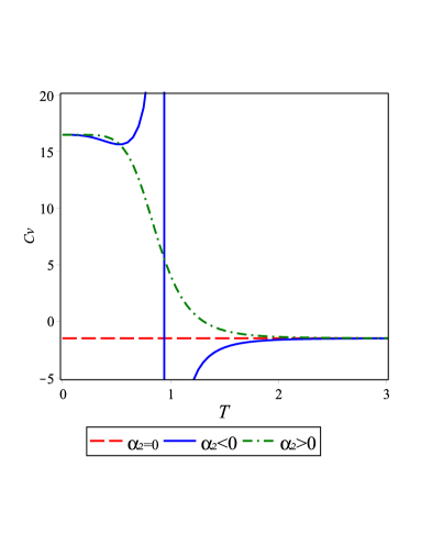
Figure 4: Typical behavior of specific heat in terms of temperature for the case of $\mathcal{B}=1$ with variation of $\alpha_{2}$. We set unit value for other parameters. $\alpha_{2}<0$ (blue solid); $\alpha_{2}=0$ (red dashed); $\alpha_{2}>0$ (dash dot green).

However, for $\mathcal{B}=1/3$, the specific heat becomes

$$C_{V}=\frac{5}{2}+\frac{18\alpha_{2}x^{2}}{(1+\alpha_{1}x+\alpha_{2}x^{2})},$$ (43)

which describes a higher-order corrected behavior of diatomic gas. The critical temperature can be obtained by maximizing $C_{V}$ as following:

$$\frac{\partial C_{V}}{\partial T}=0.$$ (44)

For $\alpha_{2}=0$, this yields to

$$2\alpha_{1}x=1.$$ (45)

For point masses galaxies, the critical temperature is given by

$$T_{c}=\left[3(Gm^{2})^{3}\frac{\bar{N}}{V}+6\left(\frac{Gm^{2}}{R}\right)^{2}\frac{\bar{N}}{V}{\int_{0}^{R}{\mathcal{F}}(r,0)r^{2}dr}\right]^{1/3}.$$ (46)

In case of extended mass galaxies, the critical temperature is given by

$$T_{c}=\left[3(Gm^{2})^{3}\frac{\bar{N}}{V}\alpha_{1}\right]^{1/3},$$ (47)

where $\alpha_{1}$ is given in (14).

For both point mass and extended mass cases, the specific heat in terms of critical temperature is expressed as

$$C_{V}=\frac{3}{2}\left[1-2\frac{1-4\left(\frac{T}{T_{c}}\right)^{3}}{\left(1+2\left(\frac{T}{T_{c}}\right)^{3}\right)^{2}}\right],$$ (48)

which matches with the expression calculated in Ref. sas2 . The above justifies that at critical temperature, the basic homogeneity of the system may break on the average of interparticle scale which has been caused by the formation of binary gravitational systems. The clustering parameter in terms of critical temperature is given by

$$\mathcal{B}=\frac{T_{c}^{3}}{T_{c}^{3}+2{T}^{3}}.$$ (49)

This shows that at $T=T_{c}$ the (critical) corrected clustering parameter ($\mathcal{B}_{crit}$) is $1/3$, at which the specific heat takes maximum value.

The pressure and internal energy, in terms of critical temperature, are written by

$$P=\frac{2N}{V}\left(\frac{T^{4}}{T_{c}^{3}+2{T}^{3}}\right),$$ (50)

$${U}=\frac{3}{2}NT\left(\frac{2T^{3}-T_{c}^{3}}{2T^{3}+T_{c}^{3}}\right).$$ (51)

Clearly, at $T=T_{c}$, the value of pressure and internal energy become $P=\frac{2}{3}\frac{NT}{V}$ and ${U}=\frac{1}{2}NT$.

VII Discussion and Conclusion

In this paper, we have investigated the higher-order correction to the partition function for the gravitational system interacting through modified gravity. We have computed all the results corresponding to modified Newtonian gravity with general correction term. It should be remembered that this model is neither suitable for the case where force is a function of the velocity of the particles nor for the case of anisotropic universe. By developing the higher-order corrected partition function, we studied the thermodynamics of galactic system. In particular, we have derived the Helmholtz free energy, Gibbs free energy, entropy, enthalpy, pressure, internal energy and the chemical potential. All of these thermodynamical quantities get correction due to the higher-order term. By comparing the expressions of these thermodynamical quantities to their standard forms, we have obtained the higher-order corrected clustering parameter which characterizes the clustering of galaxies under modified gravity. Within this context, we have discussed both the point mass and extended mass structures of galaxies. Further, we have discussed the higher-order corrected distribution function for this system. By switching-off the higher-order correction parameter, one gets the lowest order gravitational quasi-equilibrium distribution function corresponding to modified gravity.

In order to study the phase transition for galaxies evolution and cluster formation, it is important to investigate the order parameter. The behaviors of order parameter together with the conjugate field for galaxy clusters in modified gravity have found similar to that of pure Newtonian gravity case. The clustering parameter as an order parameter is related to the (so-called) critical temperature at which the specific heat takes maximum value. We have found that for modified gravitational interaction the specific heat for completely virialized system also becomes negative because bound clusters dominate. Further, we have formulated the order parameter, internal energy and the pressure in terms of the critical temperature.

- (1) G. Bertone, D. Hooper and J. Silk, Phys. Rep. 405, 279 (2004).
- (2) M. Milgrom, Astroph. J. 270, 365 (1983); 270, 371 (1983); 270, 384 (1983).
- (3) R. Sanders and S. McGaugh, Ann. Rev. Astron. Astrophys. 40, 263 (2002).
- (4) A. Yang, W. C. Saslaw, A. H. Chan, B. Leong, the Proceedings of the Conference in Honour of Murray Gell-Mann’s 80th Birthday. [arXiv:1011.0176].
- (5) T. Bernal, S. Capozziello, J. C. Hidalgo, and S. Mendoza, Eur. Phys. J. C 71, 1794 (2011).
- (6) J. D. Bekenstein, Phys.Rev.D 70, 083509 (2004).
- (7) S. M. Kent, Astron. Journ. 93, 816 (1987).
- (8) M. Milgrom, Astrophys. Journ. 333, 689 (1988).
- (9) K. G. Begeman, A. H. Broeils and R. H. Sanders, MNRAS 249, 523 (1991).
- (10) J. Ellis et al., Nucl. Phys. B 238, 453 (1984).
- (11) P. C. McGuire and P. J. Steinhardt, arXiv:astro-ph/0105567v1.
- (12) M. Byrne, C. Kolda and P. Regan, Phys. Rev. D 66, 075007 (2002).
- (13) J. Sadeghi, H. Saadat and B. Pourhassan, Chaos, Solitons and Fractals 42, 1080 (2009).
- (14) D. Benisty and E. I. Guendelman, Eur. Phys. J. C 77, 396 (2017).
- (15) E. Guendelman, E. Nissimov and S. Pacheva, Eur. Phys. J. C 75, 472 (2015).
- (16) E. Guendelman, D. Singleton and N. Yongram, JCAP 1211, 044 (2012).
- (17) E. Guendelman, E. Nissimov and S. Pacheva, Eur. Phys. J. C 76, 90 (2016).
- (18) B. Pourhassan, Physics of the Dark Universe 13, 132 (2016).
- (19) B. Pourhassan, Can. J. Phys. 94, 659 (2016).
- (20) S. Capozziello, E. De Filippis and V. Salzano, MNRAS 394, 947 (2009).
- (21) E. G. Floratos and G. K. Leontaris, Phys. Lett. B 465, 95 (1999).
- (22) J. C. Long, H. W. Chan, A. B. Churnside, E. A. Gulbis, M. C. M. Varney and J. C. Price, Nature 421, 922 (2003).
- (23) S. Capozziello and M. De Laurentis, Annalen Phys. 524, 545 (2012).
- (24) S. Capozziello, A. Stabile, A Troisi, Phys. Rev. D 76, 104019 (2007).
- (25) D. H. Eckhardt, Phys. Rev. D 48, 3762 (1993).
- (26) D. Hadjimichef and F. Kokubun, Phys. Rev. D 55, 733 (1997).
- (27) I. T. Drummond, Phys. Rev. D 63, 043503 (2001).
- (28) S. Capozziello and M. De Laurentis, Phys. Rep. 509, 167 (2011).
- (29) S. Nojiri and S.D. Odintsov, Phys. Rept. 505, 59 (2011).
- (30) B. Famaey and J. Binney, MNRAS 363, 603 (2005).
- (31) W.J.G. De Blok and S.S. McGaugh, ApJ 508, 132 (1998)
- (32) R. H. Sanders, ApJ 560, 1 (2001).
- (33) S. Capozziello, V. F. Cardone, and A. Troisi, Mon. Not. R. Astron. Soc., 375, 1423 (2007).
- (34) C. Frigerio Martins and P. Salucci, Mon. Not. R. Astron. Soc., 381, 1103 (2007).
- (35) F. C. van den Bosch and J. J. Dalcanton, ApJ 534, 146 (2000).
- (36) W. C. Saslaw and F. Ahmad, ApJ 720, 1246 (2010).
- (37) S. S. McGaugh, Phys. Rev. Lett. 106, 121303.
- (38) R. H. Sanders, MNRAS 342, 901 (2003).
- (39) M. Milgrom and R. H. Sanders, Astroph. J. 599, L25 (2003).
- (40) M. Hameeda, S. Upadhyay, M. Faizal and A. F. Ali, MNRAS 463, 3699 (2016).
- (41) M. Hameeda, M. Faizal and A. F. Ali, Gen. Rel. Grav. 48, 47 (2016).
- (42) B. Pourhassan, S. Upadhyay, M. Hameeda and M. Faizal, MNRAS 468, 3166 (2017)
- (43) S. Upadhyay, Phys. Rev. D 95, 043008 (2017).
- (44) S. Capozziello, M. Faizal, M. Hameeda, B. Pourhassan, V. Salzano and S. Upadhyay, MNRAS 474, 2430 (2018).
- (45) M. Hameeda, S. Upadhyay, M. Faizal, A. F. Ali and B. Pourhassan, arXiv:1712.08591.
- (46) M. Hessaby, Phys. Rev. 73, 1128 (1948)
- (47) T. Nakano, I. Progr. Theor. Phys. 15(4), 333 (1956)
- (48) H. Saadat and B. Pourhassan, Int. J. Theor. Phys. 55, 3827 (2016)
- (49) F. Ahmad, W.C. Saslaw, N.I. Bhat, Astrophys. J., 571, 576 (2002)
- (50) W. C. Saslaw and A. J. S. Hamilton, ApJ 13, 276 (1984).