Keep Rollin’ – Whole-Body Motion Control and Planning for Wheeled Quadrupedal Robots

Abstract

We show dynamic locomotion strategies for wheeled quadrupedal robots, which combine the advantages of both walking and driving. The developed optimization framework tightly integrates the additional degrees of freedom introduced by the wheels. Our approach relies on a zero-moment point based motion optimization which continuously updates reference trajectories. The reference motions are tracked by a hierarchical whole-body controller which computes optimal generalized accelerations and contact forces by solving a sequence of prioritized tasks including the nonholonomic rolling constraints. Our approach has been tested on ANYmal, a quadrupedal robot that is fully torque-controlled including the non-steerable wheels attached to its legs. We conducted experiments on flat and inclined terrains as well as over steps, whereby we show that integrating the wheels into the motion control and planning framework results in intuitive motion trajectories, which enable more robust and dynamic locomotion compared to other wheeled-legged robots. Moreover, with a speed of 4 m/s and a reduction of the cost of transport by 83 % we prove the superiority of wheeled-legged robots compared to their legged counterparts.

I INTRODUCTION

Wheels are one of the major technological advances of humankind. In daily life, they enable us to move faster and more efficiently as compared to legged-based locomotion. The latter, however, is more versatile and offers the possibility to negotiate challenging environments, which is why combining both strategies into one system, would achieve the best of both worlds.

While most of the advances towards autonomous mobile robots either focus on pure walking or driving, this paper shows how to plan and control trajectories for wheeled-legged robots as depicted in Fig. 1 to achieve dynamic locomotion. We believe that such kinds of systems offer the solution for many robotic tasks as described in [1], e.g., rapid exploration, payload delivery, search and rescue, and industrial inspection.

Figure 1: The fully torque-controlled quadrupedal robot ANYmal [2] is equipped with four non-steerable, torque-controlled wheels. Thus, the number of actuated joint coordinates $n_{\tau}$ and the number of joints $n_{j}$ are both equal to 16. A video demonstrating the results can be found at https://youtu.be/nGLUsyx9Vvc.

I-A Related Work

Recent years have shown an active research area focusing on the combination of wheeled and legged locomotion. Most wheeled-legged robots, such as [3, 4, 5, 6, 7, 8], behave like an active suspension system while driving and do not use their legs as a locomotion alternative to the wheels. While these wheeled-legged robots are using a kinematic approach to generate velocity commands for the wheels, there has been some promising research incorporating the whole-body dynamics of the robot to generate torque commands for each of the joints, including the wheels.

The authors in [9] show a prioritized whole-body compliant control framework that generates motor torques for the upper body of a humanoid robot attached to a wheeled base. The equations of motion, including the nonholonomic constraints, are also incorporated into the control structure of a two-wheeled mobile robot [10]. Justin [11], a wheeled humanoid robot, creates torque commands for each of the wheels using an admittance-based velocity controller. Each of these wheeled platforms, however, is not able to step due to the missing legs, and as such, the robots are only performing wheeled locomotion.

In contrast, DRC-HUBO+ [12] is a wheeled humanoid robot which is able to switch between a walking and a driving configuration. While driving, the robot is in a crouched position, and as such, the legs are not used for locomotion or balancing.

Momaro [13], on the other hand, shows driving and stepping without changing its configuration. This wheeled quadrupedal robot uses a kinematic approach to drive and to overcome obstacles like stairs and steps. Recently, the Centauro robot [14, 15, 16] showed similar results over stepping stones, steps and first attempts to overcome stairs, while performing only slow static maneuvers.

There is a clear research gap for wheeled-legged robots. Most of the robots using actuated wheels are not taking into account the dynamic model of the whole-body including the wheels. The lack of these model properties hinders these robots from performing dynamic locomotion during walking and driving. In particular, a wheeled-legged robot produces reaction forces between its wheels and the terrain to generate its motion. The switching of the legs’ contact state, the additional degrees of freedom (DOF) along the rolling direction of each wheel, and the reaction forces, all need to be accounted for in order to reveal the potential of wheeled-legged robots compared to traditional legged systems. In addition, torque control for the wheels is only explored for some slowly moving wheeled mobile platforms. Without force or torque control, the friction constraints related to the no-slip condition cannot be fulfilled, and locomotion is not robust against unknown terrain irregularities. Research areas in traditional legged locomotion [17, 2, 18, 19, 20, 21, 22], however, offer solutions to bridge these gaps. To this end, the work in [23] shows a generic approach to generate motions for wheeled-legged robots. Due to the formulation of the nonlinear programming (NLP) problem, the computation is too slow to execute in a receding horizon fashion, which is needed for robust execution under external disturbances. Moreover, the same authors verified their NLP algorithm on rather small robots.

So far, Boston Dynamics’ wheeled bipedal robot Handle [24] is the only solution that demonstrated dynamic motions to overcome high obstacles while showing adaptability against terrain irregularities. Due to the missing publications on Handle, there is no knowledge about Boston Dynamics’ locomotion framework.

I-B Contribution

This paper shows dynamic locomotion for wheeled quadrupedal robots which combine the mobility of legs with the efficiency of driving. Our main contribution is a whole-body motion control and planning framework which takes into account the additional degrees of freedom introduced by torque-controlled wheels. The motion planner relies on an online zero-moment point (ZMP) [25] based optimization which continuously updates reference trajectories for the free-floating base and the wheels in a receding horizon fashion. These optimized motion plans are tracked by a hierarchical whole-body controller (WBC) which takes into account the nonholonomic constraints introduced by the wheels. In contrast to other wheeled-legged robots, all joints including the wheels are torque controlled. To the best of our knowledge, this work shows for the first time dynamic and hybrid locomotion over flat, inclined and rough terrain for a wheeled quadrupedal robot. Moreover, we show how the same whole-body motion controller and planner are applied to driving and walking without changing any of the principles of dynamics and balance.

II MODELLING OF WHEELED-LEGGED ROBOTS

We first recall basic definitions of the kinematics and dynamics of robotic systems. Similar to walking robots [17], a wheeled-legged robot is modeled as a free-floating base $B$ to which the legs including the wheels as end-effectors are attached. Given a fixed inertial frame $I$ (see Fig. 2), the position from frame $I$ to $B$ with respect to (w.r.t.) frame $I$ and the orientation of frame $B$ w.r.t. frame $I$ are described by ${}_{I}\bm{r}_{IB}\in\mathbb{R}^{3}$ and a Hamiltonian unit quaternion $\bm{q}_{IB}$ . The generalized coordinate vector $\bm{q}$ and the generalized velocity vector $\bm{u}$ are given by

$$\bm{q}=\begin{bmatrix}{}_{I}\bm{r}_{IB}\\ \bm{q}_{IB}\\ \bm{q}_{j}\end{bmatrix}\in SE(3)\times\mathbb{R}^{n_{j}},\bm{u}=\begin{bmatrix}{}_{I}\bm{v}_{B}\\ {}_{B}\bm{\omega}_{IB}\\ \dot{\bm{q}}_{j}\end{bmatrix}\in\mathbb{R}^{n_{u}},$$ (1)

where $\bm{q}_{j}\in\mathbb{R}^{n_{j}}$ is the vector of joint coordinates, with $n_{j}$ the number of joint coordinates, $n_{u}=6+n_{j}$ is the number of generalized velocity coordinates, ${}_{I}\bm{v}_{B}\in\mathbb{R}^{3}$ is the linear velocity of frame $B$ w.r.t. frame $I$, and ${}_{B}\bm{\omega}_{IB}\in\mathbb{R}^{3}$ is the angular velocity from frame $I$ to $B$ w.r.t. frame $B$. With this convention, the equations of motion for wheeled-legged robots are defined by

$$\bm{M}(\bm{q})\dot{\bm{u}}+\bm{h}(\bm{q},\bm{u})=\bm{S}^{T}\bm{\tau}+\bm{J}_{S}^{T}\bm{\lambda},$$ (2)

where $\bm{M}(\bm{q})\in\mathbb{R}^{n_{u}\times n_{u}}$ is the mass matrix, $\bm{h}(\bm{q},\bm{u})\in\mathbb{R}^{n_{u}}$ is the vector of Coriolis, centrifugal and gravity terms, $\bm{\tau}\in\mathbb{R}^{n_{\tau}}$ is the generalized torque vector acting in the direction of the generalized coordinate vector, with $n_{\tau}$ the number of actuated joint coordinates, $\bm{J}_{S}=[\bm{J}_{C_{1}}^{T}\ {\dots}\ \bm{J}_{C_{n_{c}}}^{T}]^{T}\in\mathbb{R}^{3n_{c}\times n_{u}}$ is the support Jacobian, with $n_{c}$ the number of limbs in contact, and $\bm{\lambda}\in\mathbb{R}^{3n_{c}}$ is the vector of constraint forces. The transpose of the selection matrix $\bm{S}=[\bm{0}_{n_{\tau}\times n_{u}-n_{\tau}}\ \mathbb{I}_{n_{\tau}\times n_{\tau}}]$ maps the generalized torque vector $\bm{\tau}$ to the space of generalized forces.

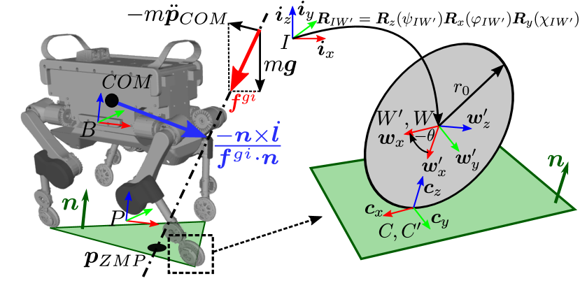
Figure 2: The figure illustrates a sketch of the wheeled quadrupedal robot ANYmal and the wheel model used to derive the rolling constraint (3). Left figure: As discussed in [17], we define a plan frame $P$ which is used as a reference frame in our motion planner. The red and blue arrows visualize the gravito-inertial wrench of the 3D ZMP model described in Section III-C3. Right figure: We differentiate between the leg-fixed and wheel-fixed coordinate frames at the wheel. The leg-fixed wheel frame $W^{\prime}$ and contact frame $C^{\prime}$ do not depend on the joint angle $\theta$ of the wheel. In contrast, the wheel-fixed wheel frame $W^{\prime}$ and contact frame $C^{\prime}$ depend on the joint angle $\theta$ of the wheel. Both contact frames are aligned with the local estimation of the terrain normal $\bm{n}$ and the rolling direction $\bm{c}_{x}$ of the wheel.

II-A Nonholonomic Rolling Constraint

In contrast to point contacts, the acceleration of the wheel-fixed contact point $C_{i}$ of the $i$-th leg does not equal zero, i.e., ${}_{I}\ddot{\bm{r}}_{IC_{i}}=\bm{J}_{C_{i}}\dot{\bm{u}}+\dot{\bm{J}}_{C_{i}}\bm{u}\neq\bm{0}$. Given the wheel model in Fig. 2, it can be shown that the resulting contact acceleration of a wheel is defined by

$${}_{I}\ddot{\bm{r}}_{IC_{i}}=\bm{J}_{C_{i}}\dot{\bm{u}}+\dot{\bm{J}}_{C_{i}}\bm{u}=$$ (3)

$$\bm{R}_{IW_{i}}\begin{bmatrix}0\\ -r_{0}\dot{\psi}_{IW^{\prime}_{i}}\cos(\varphi_{IW^{\prime}_{i}})(\dot{\chi}_{IW^{\prime}_{i}}+\dot{\theta})\\ r_{0}(\dot{\chi}_{IW^{\prime}_{i}}+\dot{\theta})(\dot{\chi}_{IW^{\prime}_{i}}+\dot{\theta}+\dot{\psi}_{IW^{\prime}_{i}}\sin(\varphi_{IW^{\prime}_{i}}))\end{bmatrix},$$

where $\bm{R}_{IW_{i}}\in SO(3)$ represents the rotation matrix that projects the components of a vector from the wheel frame $W_{i}$ to the inertial frame $I$, $r_{0}$ is the wheel radius, and $\theta_{i}$ is the joint angle of the wheel. Using an intrinsic $z-x^{\prime}-y^{\prime\prime}$ Euler parameterization, the yaw, roll, and pitch angle of the wheel fixed frame $W^{\prime}_{i}$ w.r.t. the inertial frame $I$ are given by $\psi_{IW^{\prime}_{i}}$, $\varphi_{IW^{\prime}_{i}}$, and $\chi_{IW^{\prime}_{i}}$, respectively.

By setting $\varphi_{IW^{\prime}_{i}}\equiv 0$ and $\psi_{IW^{\prime}_{i}}\equiv 0$, we obtain the acceleration for the planar case, i.e, ${}_{I}\ddot{\bm{r}}_{IC_{i}}=\bm{R}_{IW_{i}}[0\ 0\ r_{0}(\dot{\chi}_{IW^{\prime}_{i}}+\dot{\theta})^{2}]^{T}$, which is equal to the centripetal acceleration.

II-B Terrain and Contact Point Estimation

The robot is blindly locomoting on a terrain locally modeled by a three-dimensional plane. First, the terrain normal is estimated by fitting a plane through the most recent contact locations of the wheel frame $W$ in Fig. 2 using a least-squares method as described in [19]. Given the resulting terrain normal $\bm{n}$, the estimated plane is moved along the terrain normal to the contact position $C$ as illustrated in Fig. 2, i.e., the terrain plane is shifted by $\pi_{{W_{x,z}}}(-\bm{n})R/|\pi_{{W^{x,z}}}(-\bm{n})|$, where $\pi_{{W_{x,z}}}(-\bm{n})$ is the projection of the negative normal vector $\bm{n}$ onto the plane spanned by $\bm{w}_{x}$ and $\bm{w}_{z}$. Finally, the plane through the contact points represents the estimated terrain plane used for control and planning.

The leg-fixed contact frame $C^{\prime}_{i}$ and wheel-fixed contact frame $C_{i}$ of each leg $i$ are introduced to simplify the convention of the motion controller and planner. As illustrated in Fig. 2, both contact frames are defined to lie at the intersection of the wheel plane with the estimated terrain plane. The contact frame’s $z$-axis is aligned with the estimated terrain normal and its $x$-axis is perpendicular to the estimated terrain normal and aligned with the rolling direction $\bm{c}_{x}$ of the wheel.

As discussed in earlier works [17], the motion plans in Section III are computed in the plan frame $P$ whose $z$-axis is aligned with the estimated terrain normal and whose $x$-axis is perpendicular to the estimated terrain normal and aligned with the heading direction of the robot. As depicted in Fig. 2, the plan frame is located at the footprint center projected onto the local terrain along the terrain normal.

III MOTION PLANNING

The dynamic model of a wheeled-legged robot (2) includes significant nonlinearities to be handled by the motion planner. Due to this complexity, the optimization problem becomes prone to local minima and it can be demanding to solve in real-time on-board [20]. To overcome these challenges, our approach breaks down the whole-body planning problem into center of mass (COM) and foothold motion optimization [17, 26]. We simplify the system dynamics to a ZMP model for motion planning of the COM. The reference footholds for each leg are obtained by solving a separate optimization problem.

Fig. 3 gives an overview of the entire whole-body motion control and planning framework. The foothold optimizer, motion optimizer, and WBC modules are solving separate optimization problems in parallel such that there is no interruption between them [17]. We generate all motions w.r.t. the plan frame $P$ introduced in Section II-B. In the following, we describe each module of the motion planner.

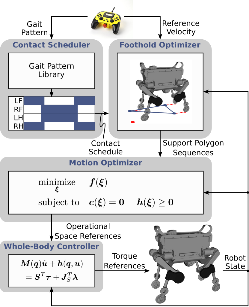
Figure 3: The motion planner is based on a 3D ZMP approach which takes into account the support polygon sequence and the state of the robot. The hierarchical WBC which optimizes the whole-body accelerations and contact forces tracks the operational space references. Finally, torque references are sent to the robot.

III-A Contact Scheduler

The contact schedule defines periodic sequences of lift-off and touch-down events for each leg. Based on a gait pattern library, each gait predefines the timings for each leg over a stride, e.g., the contact scheduler block in Fig. 3 illustrates the gait pattern for a trotting gait. With this formulation, driving is defined by a gait pattern where each leg is scheduled to stay in contact, and no lift-off events are set.

III-B Foothold Optimizer

Given a reference in terms of linear velocity $\bm{v}_{B}^{ref}=[v_{B,x}^{ref}\ v_{B,y}^{ref}\ 0]^{T}$ and angular velocity $\bm{\omega}_{B}^{ref}=[0\ 0\ \omega_{B,z}^{ref}]^{T}$ of the base, and the contact schedule, desired footholds are generated for each leg. Based on the contact schedule and footholds, a sequence of support polygons are generated, where each polygon is defined by the convex hull of expected footholds, e.g., the green polygon in Fig. 2, as well as its time duration in seconds.

While walking, we formulate a quadratic programming (QP) problem which optimizes over the $x$ and $y$ coordinates of each foothold [17]. Costs, which are added to the QP problem, penalize the distance between the optimized foothold locations and different contributions to the computation of the footholds. We assign default foothold positions which define the standing configuration of the robot. Footholds are projected using the high-level reference velocity and assuming constant reference velocity throughout the optimization horizon. To ensure smoothness of the footholds, we penalize the deviation from previously computed footholds. Finally, we rely on an inverted pendulum model to stabilize the robot’s motion [19]. Inequality constraints are added to avoid collisions of the feet and to respect the maximum kinematic extension of each leg. Given the previous stance foot position and the optimized foothold, a swing trajectory for each leg is generated by fitting a spline between both.

Traditional legged locomotion is based on the constraint that the leg-fixed contact point $C^{\prime}$ remains stationary when in contact with the environment. In contrast, wheeled-legged robots are capable of executing trajectories along the rolling direction $\bm{c}_{x}$ of the wheel. This can be seen as a moving foothold. While driving, the desired leg-fixed contact position ${}_{I}\bm{r}_{IC^{\prime}_{i}}^{d}\in\mathbb{R}^{3}$, velocity ${}_{I}\dot{\bm{r}}_{IC^{\prime}_{i}}^{d}\in\mathbb{R}^{3}$ and acceleration ${}_{I}\ddot{\bm{r}}_{IC^{\prime}_{i}}^{d}\in\mathbb{R}^{3}$ of leg $i$ are computed based on the reference velocities $\bm{v}_{B}^{ref}$ and $\bm{\omega}_{B}^{ref}$ of the base and the state of the robot.

III-C Motion Optimizer

The motion optimizer generates operational space references for the $x$, $y$ and $z$ coordinates of the whole-body COM given the support polygon sequence and the robot state [17]. The resulting nonlinear optimization framework is described in the following sections.

III-C1 Motion plan parameterization

The $x$, $y$, and $z$ coordinates of the COM trajectory are parametrized as a sequence of quintic splines [17], i.e., the position, velocity and acceleration of the COM are given by $\bm{p}_{COM}=\bm{T}(t)\bm{\alpha}_{k}\in\mathbb{R}^{3}$, $\dot{\bm{p}}_{COM}=\dot{\bm{T}}(t)\bm{\alpha}_{k}\in\mathbb{R}^{3}$, and $\ddot{\bm{p}}_{COM}=\ddot{\bm{T}}(t)\bm{\alpha}_{k}\in\mathbb{R}^{3}$, with $\bm{T}(t)=diag(\bm{\eta}^{T}(t),\bm{\eta}^{T}(t),\bm{\eta}^{T}(t))\in\mathbb{R}^{3\times 18}$, $\bm{\eta}^{T}(t)=[t^{5}\ t^{4}\ t^{3}\ t^{2}\ t\ 1]$, $t\in[\bar{t},\bar{t}+\Delta t_{k}]$, where $\bar{t}$ is the sum of time durations of all previous splines, and $\Delta t_{k}$ is the time duration of the $k$-th spline. All coefficients of spline $i$ are stored in $\bm{\alpha}_{k}=[{\bm{\alpha}_{k}^{x}}^{T}\ {\bm{\alpha}_{k}^{y}}^{T}\ {\bm{\alpha}_{k}^{z}}^{T}]^{T}\in\mathbb{R}^{18}$. Finally, we solve for the vector of optimization parameters which is obtained by stacking together all spline coefficient vectors $\bm{\alpha}_{k}$.

III-C2 Optimization problem

The motion optimization problem is expressed as a nonlinear optimization problem with objective $\bm{f}(\bm{\xi})$, equality constraints $\bm{c}(\bm{\xi})$, and inequality constraints $\bm{h}(\bm{\xi})$. The problem is described by

$$\underset{\bm{\xi}}{\text{minimize}} \bm{f}(\bm{\xi})$$ (4)

subject to $$\bm{c}(\bm{\xi})=\bm{0},\ \ \ \ \bm{h}(\bm{\xi})\geq\bm{0},$$

where $\bm{\xi}$ is the vector of optimization variables given in Section III-C1, i.e., optimal spline coefficients are computed. A sequential quadratic programming (SQP) algorithm [27] is used to solve (4) continuously over a time horizon of $\tau$ seconds. Table I summarizes each objective and constraint used in this work.

TABLE I: The table lists the costs and constraints of the motion optimization problem based on [17].

Type	Task	Purpose
Objective	Minimize COM acceleration	Smooth motions
Objective	Minimize deviation to previous solution $\bm{\xi}_{prev}$	Smooth motions
Objective	Track a high-level reference trajectory $\bm{\pi}$ (path regularizer) $\forall\,\bm{\xi}$	Reference tracking
Soft constraint (lin.-quad.)	Minimize deviation to initial & final conditions $\forall\,\bm{\xi}$	Disturbance rejection & reference tracking
Soft constraint (lin.-quad.)	Limit overshoots $\forall\,\bm{\xi}^{z}$	Avoid kinematic limits of legs
Constraint (lin. eq.)	Junction constraints $\forall$ pairs of adjacent splines $k$, $k+1$ $\forall\,\bm{\xi}$	Continuity
Constraint (lin. ineq.)	Push Contact Constraints	Legs can only push the ground
Constraint (nonlin. ineq.)	ZMP criterion	Stability
Soft constraint (nonlin.)	Soften initial ZMP constraints	Relaxation

III-C3 ZMP inequality constraint

To ensure dynamic stability of the planned motions, an inequality constraint on the ZMP position $\bm{p}_{ZMP}\in\mathbb{R}^{3}$ is included in the motion optimization, where $\bm{p}_{ZMP}=\bm{n}\times\bm{m}_{O}^{gi}/(\bm{n}^{T}\bm{f}^{gi})$ [28]. Here, $\bm{m}_{O}^{gi}\in\mathbb{R}^{3}$ and $\bm{f}^{gi}\in\mathbb{R}^{3}$ are the components of the gravito-inertial wrench [29], with $\bm{m}_{O}^{gi}=m\cdot\bm{p}_{COM}\times(\bm{g}-\ddot{\bm{p}}_{COM})-\dot{\bm{l}}$ and $\bm{f}^{gi}=m\cdot(\bm{g}-\ddot{\bm{p}}_{COM})$, where $m$ is the mass of the robot, $\bm{l}\in\mathbb{R}^{3}$ is the angular momentum of the COM, and $\bm{g}\in\mathbb{R}^{3}$ is the gravity vector. Fig. 2 shows a sketch of the gravito-inertial wrench acting at the COM. As in [17], we assume that $\dot{\bm{l}}=\bm{0}$.

As illustrated in Fig. 2, the ZMP position $\bm{p}_{ZMP}$ is constrained to lie inside the support polygon. This stability criterion is formulated as a nonlinear inequality constraint given by [17]

$$\begin{bmatrix}p&q&0\end{bmatrix}\bm{p}_{ZMP}+r\geq 0,$$ (5)

where $\bm{d}=[p\ q\ r]^{T}$ are the coefficients of the line that goes through the edge of a support polygon.

III-C4 Deformation of support polygons while driving

In contrast to point feet, the contact locations, and therefore footholds, are not stationary while driving. The support polygon sequence which is needed to fulfill the inequality constraint in (5) is deformed over time. For this purpose, we assume that the number of edges stays constant and therefore, one spline is sufficient to describe the motion of the COM.

First, the expected foothold position for the optimization horizon $\tau$ is computed as a function of the reference velocities $\bm{v}_{B}^{ref}$ and $\bm{\omega}_{B}^{ref}$. The reference velocities are assumed to be constant over the optimization horizon. Using the time-integrated Rodriguez’s formula, the expected foothold position $\bm{p}_{\tau,i}\in\mathbb{R}^{3}$ of leg $i$ is computed by

$$\bm{p}_{\tau,i}=\bm{p}_{0,i}+\bm{R}(\tau\bm{\omega}_{B}^{ref})$$ (6)

$$\frac{1}{\omega_{B,z}^{ref}}\begin{bmatrix}\sin(\omega_{B,z}^{ref}\tau)&-1+\cos(\omega_{B,z}^{ref}\tau)&0\\ 1-\cos(\omega_{B,z}^{ref}\tau)&\sin(\omega_{B,z}^{ref}\tau)&0\\ 0&0&0\end{bmatrix}\bm{v}_{B}^{ref},$$

where $\bm{p}_{0,i}\in\mathbb{R}^{3}$ is the current foothold position. If $\omega_{B,z}^{ref}\approx 0$, the solution becomes $\bm{p}_{\tau,i}=\bm{p}_{0,i}+\tau\bm{v}_{B}^{ref}$.

Given the coefficients which describe an edge that belongs to the current and expected support polygon, i.e., $\bm{d}_{0}\in\mathbb{R}^{3}$ and $\bm{d}_{\tau}\in\mathbb{R}^{3}$, the deformed edge coefficient vector $\bm{d}_{k}(t)$ at time $t$ is computed by interpolating $\bm{d}_{0}$ and $\bm{d}_{\tau}$, i.e.,

$$\bm{d}(t)=(1-\frac{t-\bar{t}}{\tau})\bm{d}_{\tau}+\frac{t-\bar{t}}{\tau}\bm{d}_{0}.$$ (7)

IV WHOLE-BODY CONTROLLER

The operational space reference trajectories of the COM and wheels are tracked by a WBC which is based on the hierarchical optimization (HO) framework described in [17, 26]. We compute optimal generalized accelerations $\dot{\bm{u}}^{*}$ and contact forces $\bm{\lambda}^{*}$ which are collected in the vector of optimization variables $\bm{\xi}^{*}=[\dot{\bm{u}}^{*T}\ \bm{\lambda}^{*T}]^{T}\in\mathbb{R}^{n_{u}+3n_{c}}$, where all symbols are introduced in Section II.

The WBC is formulated as a cascade of QP problems composed of linear equality and inequality tasks, which are solved in a strict prioritized order [30]. A task $T_{p}$ with priority $p$ is defined by

$$T_{p}:\begin{cases}\bm{W}_{eq,p}(\bm{A}_{p}\bm{\xi}-\bm{b}_{p})=\bm{0}\\ \bm{W}_{ineq,p}(\bm{D}_{p}\bm{\xi}-\bm{f}_{p})\leq\bm{0}\end{cases},$$ (8)

where the linear equality constraints are defined by $\bm{A}_{p}$ and $\bm{b}_{p}$, the linear inequality constraints are defined by $\bm{D}_{p}$ and $\bm{f}_{p}$, and the diagonal positive-definite matrices $\bm{W}_{eq,p}$ and $\bm{W}_{ineq,p}$ weigh tasks on the same priority level.

TABLE II: The table lists the prioritized tasks (priority 1 is the highest) used in the WBC. Bold tasks are tailored for wheeled-legged robots.

Priority	Task
1	Floating base equations of motion
	Torque limits and friction cone
	Nonholonomic rolling constraint
2	COM linear and angular motion tracking
	Swing leg motion tracking
	Swing wheel rotation minimization
	Ground leg motion tracking
3	Contact force minimization

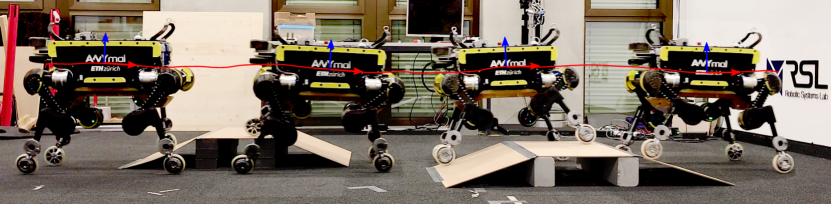
Figure 4: The robot ANYmal drives with a speed of 0.7 m/s. over two inclines of a height of approximately 30 % of ANYmal’s leg length and the red line depicts the COM trajectory (Available at https://youtu.be/nGLUsyx9Vvc?t=20).

IV-A Prioritized Tasks

The highlighted tasks in Table II are specifically tailored for wheeled-legged robots, and the following sections describe each of these tasks in more detail. For the remaining tasks, we rely on the same implementation as used for traditional legged robots [26].

Floating base equations of motion: The optimization vector $\bm{\xi}$ is constrained to be consistent with the system dynamics.

Torque limits and friction cone: Inequality constraint tasks are added to the optimization problem to avoid that the computed torques exceed the minimum and maximum limit of each actuator. Similar, the contact forces $\bm{\lambda}$ need to lie inside the friction cone which is approximated by a friction pyramid and aligned with the normal vector $\bm{n}$ of the estimated contact surface shown in Fig. 2.

Nonholonomic rolling constraint: The solution found by the optimization needs to take into account the nonholonomic rolling constraint (3). This is expressed as an equality constraint given by

$$\begin{bmatrix}\bm{J}_{S}&\bm{0}_{3n_{c}\times 3n_{c}}\end{bmatrix}\bm{\xi}_{d}=-\dot{\bm{J}}_{S}\bm{u}+\begin{bmatrix}{}_{I}\ddot{\bm{r}}_{IC_{1}}^{T}&{\dots}&{}_{I}\ddot{\bm{r}}_{IC_{n_{c}}}^{T}\end{bmatrix}^{T},$$ (9)

where the terms ${}_{I}\ddot{\bm{r}}_{IC_{1}}\ {\dots}\ _{I}\ddot{\bm{r}}_{IC_{n_{c}}}$ on the right side of the equation are the centripetal accelerations of each contact point $n_{c}$ derived in (3).

COM linear and angular motion tracking: Similar to the swing leg motion tracking task, the operational space references of the COM are tracked by equality constraint tasks.

Swing leg motion tracking: Given the operational space references of the wheels’ contact points ${}_{P}\bm{r}_{IC^{\prime}_{i}}^{d}$, ${}_{P}\dot{\bm{r}}_{IC^{\prime}_{i}}^{d}$, and ${}_{P}\ddot{\bm{r}}_{IC^{\prime}_{i}}^{d}$, the motion tracking task of each swing leg $i$ is formulated by

$$\begin{bmatrix}\bm{J}_{C^{\prime}_{i}}&\bm{0}_{3n_{c}\times 3n_{c}}\end{bmatrix}\bm{\xi}_{d}= \bm{R}_{IP}({{}_{P}\ddot{\bm{r}}_{IC^{\prime}_{i}}^{d}}+\bm{K}_{p}({{}_{P}\bm{r}_{IC^{\prime}_{i}}^{d}}-{{}_{P}\bm{r}_{IC^{\prime}_{i}}})$$ (10)

$$+\bm{K}_{d}({{}_{P}\dot{\bm{r}}_{IC^{\prime}_{i}}^{d}}-{{}_{P}\dot{\bm{r}}_{IC^{\prime}_{i}}}))-\dot{\bm{J}}_{C^{\prime}_{i}}\bm{u},$$

where $\bm{K}_{p},\bm{K}_{d}\in\mathbb{R}^{3\times 3}$ are diagonal positive definite matrices which define proportional and derivative gains. Note that all measured values, i.e., $\bm{J}_{C^{\prime}_{i}}$, ${}_{P}\bm{r}_{IC^{\prime}_{i}}$, and ${}_{P}\dot{\bm{r}}_{IC^{\prime}_{i}}$, are independent of the wheel angle $\theta$ (as discussed in the footnotes of Section II-A).

Swing wheel rotation minimization: For each swing leg $i$, the wheel’s rotation is damped by adding the task

$$\begin{bmatrix}\bm{S}_{W_{i}}&\bm{0}_{3n_{c}\times 3n_{c}}\end{bmatrix}\bm{\xi}_{d}=-k_{d}\dot{\theta}_{i},$$ (11)

where $\bm{S}_{W_{i}}\in\mathbb{R}^{3n_{c}\times n_{u}}$ is a matrix which selects the row of $\bm{\xi}_{d}$ containing the wheel of leg $i$, $k_{d}$ is a derivative gain, and $\dot{\theta}_{i}$ is the wheel’s rotational speed.

Ground leg motion tracking: To track the desired motion of the grounded legs, we constrain the accelerations in the direction of the rolling direction $\bm{c}_{x}$. Given the operational space references of the wheels’ contact points ${}_{P}\bm{r}_{IC^{\prime}_{i}}^{d}$, ${}_{P}\dot{\bm{r}}_{IC^{\prime}_{i}}^{d}$, and ${{}_{P}\ddot{\bm{r}}_{IC^{\prime}_{i}}^{d}}$, the motion tracking task of each ground leg $i$ is formulated by

$$\begin{aligned} &\pi_{\bm{c}_{x}}(\begin{bmatrix}\bm{J}_{C^{\prime}_{i}}&\bm{0}_{3n_{c}\times 3n_{c}}\end{bmatrix}\bm{\xi}_{d})=\pi_{\bm{c}_{x}}(\bm{R}_{IP}({{}_{P}\ddot{\bm{r}}_{IC^{\prime}_{i}}^{d}}\\ &+\bm{K}_{p}({{}_{P}\bm{r}_{IC^{\prime}_{i}}^{d}}-{{}_{P}\bm{r}_{IC^{\prime}_{i}}})+\bm{K}_{d}({{}_{P}\dot{\bm{r}}_{IC^{\prime}_{i}}^{d}}-{{}_{P}\dot{\bm{r}}_{IC^{\prime}_{i}}}))-\dot{\bm{J}}_{C^{\prime}_{i}}\bm{u}),\end{aligned},$$ (12)

where $\pi_{\bm{c}_{x}}(\bm{a})$ is the projection of a vector $\bm{a}$ onto the vector $\bm{c}_{x}$.

Contact force minimization: Finally, the contact forces $\bm{\lambda}$ are minimized to reduce slippage.

IV-B Torque Generation

Given the optimal solution $\bm{\xi}^{*}$, the desired actuation torques $\bm{\tau}_{d}$, which are sent to the robot, are computed by

$$\bm{\tau}_{d}=\bm{M}_{j}(\bm{q})\dot{\bm{u}}^{*}+\bm{h}_{j}(\bm{q},\bm{u})-\bm{J}_{Sj}^{T}\bm{\lambda^{*}},$$ (13)

where $\bm{M}_{j}(\bm{q})$, $\bm{h}_{j}(\bm{q},\bm{u})$, and $\bm{J}_{Sj}$ are the lower rows of the equations of motion in (2) relative to the actuated joints.

V EXPERIMENTAL RESULTS AND DISCUSSION

To show the benefits and validity of our new approach, this section reports on experiments conducted on a real quadrupedal robot equipped with non-steerable, torque-controlled wheels. The robot is driven using external velocity inputs coming from a joystick. All computation was carried out by the PC (Intel i7-5600U, 2.6 - 3.2GHz, dual-core 64-bit) integrated into the robot. A video showing the results accompanies this paper.

The WBC runs together with state estimation in a 400 Hz loop. A novel state estimation algorithm based on [31] is used to generate an estimation of the robot’s position, velocity, and orientation w.r.t. an inertial coordinate frame. Similar to [32], we fuse data from an inertial measurement unit (IMU) as well as the kinematic measurements from each actuator (including the wheels) to acquire a fast state estimation of the robot. The open-source Rigid Body Dynamics Library [33] (RBDL) is used for modeling and computation of kinematics and dynamics based on the algorithms described in [34]. We use a custom SQP algorithm to solve the nonlinear optimization problem in Section III-C2, which solves the nonlinear problem by iterating through a sequence of QP problems. Each QP problem is solved using QuadProg++ [35] which uses the Goldfarb-Idnani active-set method [36]. Depending on the gait, the motion optimization in Section III-C runs between 100 and 200 Hz.

V-A Indoor Environment: Flat Terrain

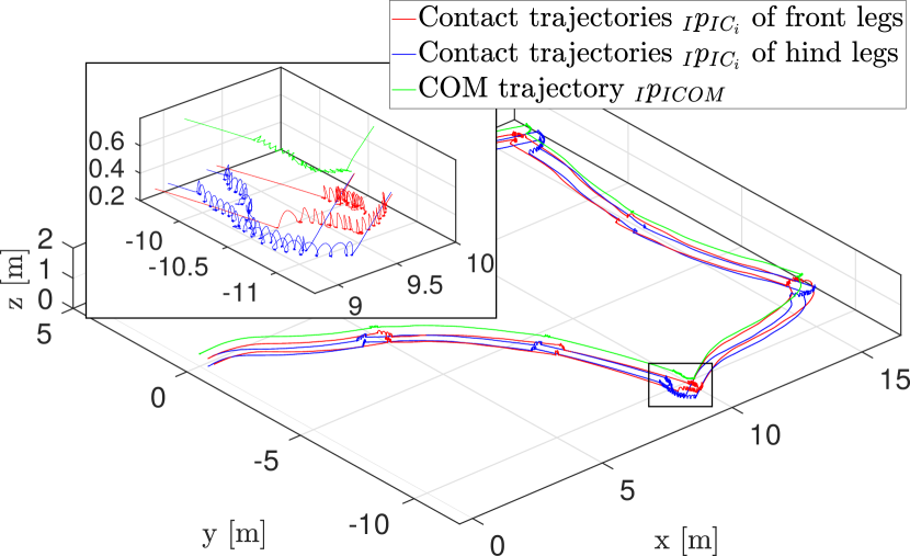
Figure 5: The robot ANYmal is driving and walking in an indoor environment (Available at https://youtu.be/nGLUsyx9Vvc?t=103). The three-dimensional plot shows estimated measurements of the robot where the red, blue and green lines depict the contact trajectories of the front legs, the contact trajectories of the hind legs, and the COM trajectories w.r.t. the inertial frame $I$. The zoomed-in figure shows transitions between driving and walking while the robot is performing a 90 degrees turn.

We performed driving and walking in an indoor environment, and the results are illustrated in Fig. 5. The three-dimensional plot shows the measured trajectories of the front legs, hind legs, and the COM. In addition, the zoomed-in plot depicts the transitions between driving and walking in a corner. As discussed in [37], the robot is able to drive small curvatures although the robot is equipped with non-steerable wheels. By yawing the base of the robot, the wheels are turning w.r.t. an inertial frame. For larger curvatures, the robot needs to step. The results successfully prove the omnidirectional capabilities of the robot.

V-B Indoor Environment: Inclined Terrain

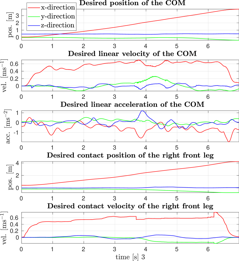
Figure 6: The plots show the desired motion (i.e., the optimized trajectories of the motion planner) of the COM and the right front leg during the driving maneuver in Fig. 4 (Available at https://youtu.be/nGLUsyx9Vvc?t=20). The executed trajectories are almost identical to the desired motion shown here, and thus, the tracking error is negligible. This is due to the fast update rate (up to 200 Hz) of the motion optimizer and the reinitialization of the optimization problem after every iteration with the measured state of the robot.

Fig. 4 depicts the COM motion tracked by the controller while ANYmal is driving blindly over two inclines and Fig. 6 illustrates the optimized trajectories of the motion planner while driving over the inclined terrain. Thanks to torque control, the robot adapts naturally to the unseen terrain irregularities while maintaining the COM height. Moreover, the COM motion is unaffected by the two obstacles although the robot drives at a speed of 0.7 m/s. In addition, none of the wheels violates the friction constraints related to the no-slip condition.

V-C Outdoor Environment: Crossing a Street

We conducted an outdoor experiment where we validated the performance of the robot under real-world conditions. Since the robot is able to drive fast and efficiently while being able to overcome obstacles, it applies to real-world tasks such as payload delivery. For this purpose, we conducted an experiment where the robot’s task is to cross a street. As can be seen in Fig. 7, the robot is able to drive down a step and to walk over another one. In addition, the lower left image illustrates how the robot rotates its base around the yaw direction to change its driving direction. This experiment also highlights the significant advantages of wheeled-legged robots compared to traditional walking robots. The robot is able to drive down steps with 1 m/s without the need for terrain perception. Moreover, the lower right image of Fig. 7, which shows the robot driving down a stair with 1 m/s without the need to step, confirms the advantage.

V-D High Speed and Low Cost of Transport

The computation of the mechanical cost of transport (COT) is based on the work in [37]. On flat terrain, the robot achieves a COT of 0.1 while driving 2 m/s and the mechanical power consumption is 63.64 W. A comparison to traditional walking and skating with passive wheels [37] shows that the COT is lower by 83 % w.r.t. the trotting gait and by 17 % w.r.t. skating motions. In addition, with 4 m/s we broke ANYmal’s maximum speed record of 1.5 m/s given in [38].

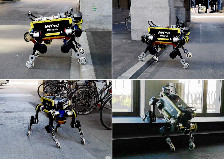
Figure 7: The figure illustrates several skills of the wheeled version of ANYmal (Available at https://youtu.be/nGLUsyx9Vvc?t=38 and https://youtu.be/nGLUsyx9Vvc?t=5): dynamically driving down a step with 1 m/s (top left image), walking up a step (top right image), driving in a curve by yawing the base (lower left image), and dynamically driving down stairs with 1 m/s (lower right image).

VI CONCLUSIONS

In this work, we show a whole-body motion control and planning framework for a quadrupedal robot equipped with non-steerable, torque-controlled wheels as end-effectors. The mobile platform combines the advantages of legged and wheeled robots. In contrast to other wheeled-legged robots, we show for the first time dynamic motions over flat and inclined terrains as well as over steps. These are enabled thanks to the tight integration of the wheels into the motion planning and control framework. For the motion optimization, we rely on a 3D ZMP approach which updates the motion plan continuously. This motion plan is tracked by a hierarchical WBC which considers the nonholonomic contact constraint introduced by the wheels. Thanks to torque control, the robot does not violate the contact constraints and the fast update rates of the motion control and planning framework make the robot robust in the face of unpredictable terrain.

We aim to demonstrate further the application of the system to real-world tasks by conducting additional outdoor experiments. Future research will focus on hybrid locomotion strategies, i.e., walking and driving at the same time. To this end, promising initial results of a novel trajectory optimization for wheeled-legged quadrupedal robots further expand on the current motion planner presented by optimizing both COM and foot trajectories in a single optimization using linearized ZMP constraints [39]. In addition, perceptive motion planning over a long time horizon in challenging environments is still an unsolved problem for wheeled-legged and legged robots.

References

- [1] C. D. Bellicoso, M. Bjelonic, L. Wellhausen, K. Holtmann, F. Günther, M. Tranzatto, P. Fankhauser, and M. Hutter, “Advances in real-world applications for legged robots,” Journal of Field Robotics, vol. 35, no. 8, pp. 1311–1326, 2018.
- [2] M. Hutter, C. Gehring, D. Jud, A. Lauber, C. D. Bellicoso, V. Tsounis, J. Hwangbo, K. Bodie, P. Fankhauser, M. Bloesch, et al., “ANYmal - a highly mobile and dynamic quadrupedal robot,” in IEEE/RSJ International Conference on Intelligent Robots and Systems (IROS), 2016, pp. 38–44.
- [3] W. Reid, F. J. Pérez-Grau, A. H. Göktoğan, and S. Sukkarieh, “Actively articulated suspension for a wheel-on-leg rover operating on a martian analog surface,” in IEEE International Conference on Robotics and Automation (ICRA), 2016, pp. 5596–5602.
- [4] P. R. Giordano, M. Fuchs, A. Albu-Schaffer, and G. Hirzinger, “On the kinematic modeling and control of a mobile platform equipped with steering wheels and movable legs,” in IEEE International Conference on Robotics and Automation, 2009, pp. 4080–4087.
- [5] F. Cordes, C. Oekermann, A. Babu, D. Kuehn, T. Stark, F. Kirchner, and D. R. I. C. Bremen, “An active suspension system for a planetary rover,” in Proceedings of the International Symposium on Artificial Intelligence, Robotics and Automation in Space (i-SAIRAS), 2014, pp. 17–19.
- [6] M. Giftthaler, F. Farshidian, T. Sandy, L. Stadelmann, and J. Buchli, “Efficient kinematic planning for mobile manipulators with non-holonomic constraints using optimal control,” in IEEE International Conference on Robotics and Automation (ICRA), 2017, pp. 3411–3417.
- [7] A. Suzumura and Y. Fujimoto, “Real-time motion generation and control systems for high wheel-legged robot mobility,” IEEE Transactions on Industrial Electronics, vol. 61, no. 7, pp. 3648–3659, 2014.
- [8] C. Grand, F. Benamar, and F. Plumet, “Motion kinematics analysis of wheeled–legged rover over 3d surface with posture adaptation,” Mechanism and Machine Theory, vol. 45, no. 3, pp. 477–495, 2010.
- [9] L. Sentis, J. Petersen, and R. Philippsen, “Implementation and stability analysis of prioritized whole-body compliant controllers on a wheeled humanoid robot in uneven terrains,” Autonomous Robots, vol. 35, no. 4, pp. 301–319, 2013.
- [10] S. Jeong and T. Takahashi, “Wheeled inverted pendulum type assistant robot: design concept and mobile control,” Intelligent Service Robotics, vol. 1, no. 4, pp. 313–320, 2008.
- [11] A. Dietrich, K. Bussmann, F. Petit, P. Kotyczka, C. Ott, B. Lohmann, and A. Albu-Schäffer, “Whole-body impedance control of wheeled mobile manipulators,” Autonomous Robots, vol. 40, no. 3, pp. 505–517, 2016.
- [12] J. Lim, I. Lee, I. Shim, H. Jung, H. M. Joe, H. Bae, O. Sim, J. Oh, T. Jung, S. Shin, et al., “Robot system of DRC-HUBO+ and control strategy of team kaist in darpa robotics challenge finals,” Journal of Field Robotics, vol. 34, no. 4, pp. 802–829, 2017.
- [13] T. Klamt and S. Behnke, “Anytime hybrid driving-stepping locomotion planning,” in International Conference on Intelligent Robots and Systems (IROS), 2017, pp. 4444–4451.
- [14] T. Klamt, D. Rodriguez, M. Schwarz, C. Lenz, D. Pavlichenko, D. Droeschel, and S. Behnke, “Supervised autonomous locomotion and manipulation for disaster response with a centaur-like robot,” in IEEE/RSJ International Conference on Intelligent Robots and Systems (IROS), 2018, pp. 1–8.
- [15] A. Laurenzi, E. M. Hoffman, and N. G. Tsagarakis, “Quadrupedal walking motion and footstep placement through linear model predictive control,” in IEEE/RSJ International Conference on Intelligent Robots and Systems (IROS), 2018, pp. 2267–2273.
- [16] M. Kamedula, N. Kashiri, and N. G. Tsagarakis, “On the kinematics of wheeled motion control of a hybrid wheeled-legged centauro robot,” in IEEE/RSJ International Conference on Intelligent Robots and Systems (IROS), 2018, pp. 2426–2433.
- [17] C. D. Bellicoso, F. Jenelten, C. Gehring, and M. Hutter, “Dynamic locomotion through online nonlinear motion optimization for quadrupedal robots,” IEEE Robotics and Automation Letters, vol. 3, no. 3, pp. 2261–2268, 2018.
- [18] J. Pratt, P. Dilworth, and G. Pratt, “Virtual model control of a bipedal walking robot,” in IEEE International Conference on Robotics and Automation (ICRA), vol. 1, 1997, pp. 193–198.
- [19] C. Gehring, S. Coros, M. Hutter, C. D. Bellicoso, H. Heijnen, R. Diethelm, M. Bloesch, P. Fankhauser, J. Hwangbo, M. Hoepflinger, et al., “Practice makes perfect: An optimization-based approach to controlling agile motions for a quadruped robot,” IEEE Robotics & Automation Magazine, vol. 23, no. 1, pp. 34–43, 2016.
- [20] G. Bledt, P. M. Wensing, and S. Kim, “Policy-regularized model predictive control to stabilize diverse quadrupedal gaits for the mit cheetah,” in IEEE/RSJ International Conference on Intelligent Robots and Systems (IROS), 2017, pp. 4102–4109.
- [21] H.-W. Park, P. M. Wensing, and S. Kim, “High-speed bounding with the mit cheetah 2: Control design and experiments,” The International Journal of Robotics Research, vol. 36, no. 2, pp. 167–192, 2017.
- [22] A. W. Winkler, C. D. Bellicoso, M. Hutter, and J. Buchli, “Gait and trajectory optimization for legged systems through phase-based end-effector parameterization,” IEEE Robotics and Automation Letters, vol. 3, no. 3, pp. 1560–1567, 2018.
- [23] M. Geilinger, R. Poranne, R. Desai, B. Thomaszewski, and S. Coros, “Skaterbots: Optimization-based design and motion synthesis for robotic creatures with legs and wheels,” ACM Transactions on Graphics (TOG), vol. 37, no. 4, p. 160, 2018.
- [24] Boston Dynamics. Introducing handle. Youtube. [Online]. Available: https://www.youtube.com/watch?v=-7xvqQeoA8c
- [25] M. Vukobratović and B. Borovac, “Zero-moment point – thirty five years of its life,” International journal of humanoid robotics, vol. 1, no. 01, pp. 157–173, 2004.
- [26] C. D. Bellicoso, F. Jenelten, P. Fankhauser, C. Gehring, J. Hwangbo, and M. Hutter, “Dynamic locomotion and whole-body control for quadrupedal robots,” in IEEE/RSJ International Conference on Intelligent Robots and Systems (IROS), 2017, pp. 3359–3365.
- [27] P. T. Boggs and J. W. Tolle, “Sequential quadratic programming,” Acta numerica, vol. 4, pp. 1–51, 1995.
- [28] P. Sardain and G. Bessonnet, “Forces acting on a biped robot. center of pressure-zero moment point,” IEEE Transactions on Systems, Man, and Cybernetics-Part A: Systems and Humans, vol. 34, no. 5, pp. 630–637, 2004.
- [29] S. Caron, Q.-C. Pham, and Y. Nakamura, “Zmp support areas for multicontact mobility under frictional constraints,” IEEE Transactions on Robotics, vol. 33, no. 1, pp. 67–80, 2017.
- [30] C. D. Bellicoso, C. Gehring, J. Hwangbo, P. Fankhauser, and M. Hutter, “Perception-less terrain adaptation through whole body control and hierarchical optimization,” in IEEE-RAS International Conference on Humanoid Robots (Humanoids), 2016, pp. 558–564.
- [31] M. Bloesch, M. Burri, H. Sommer, R. Siegwart, and M. Hutter, “The two-state implicit filter recursive estimation for mobile robots,” IEEE Robotics and Automation Letters, vol. 3, no. 1, pp. 573–580, 2018.
- [32] M. Bloesch, M. Hutter, M. A. Hoepflinger, S. Leutenegger, C. Gehring, C. D. Remy, and R. Siegwart, “State estimation for legged robots-consistent fusion of leg kinematics and imu,” Robotics, vol. 17, pp. 17–24, 2013.
- [33] M. Felis. Rigid Body Dynamics Library. [Online]. Available: https://bitbucket.org/rbdl/rbdl/src/default/
- [34] R. Featherstone, Rigid body dynamics algorithms. Springer, 2014.
- [35] L. D. Gasper. QuadProg++. [Online]. Available: http://quadprog.sourceforge.net/
- [36] D. Goldfarb and A. Idnani, “A numerically stable dual method for solving strictly convex quadratic programs,” Mathematical programming, vol. 27, no. 1, pp. 1–33, 1983.
- [37] M. Bjelonic, C. D. Bellicoso, M. E. Tiryaki, and M. Hutter, “Skating with a force controlled quadrupedal robot,” in IEEE/RSJ International Conference on Intelligent Robots and Systems (IROS), 2018, pp. 7555–7561.
- [38] J. Hwangbo, J. Lee, A. Dosovitskiy, D. Bellicoso, V. Tsounis, V. Koltun, and M. Hutter, “Learning agile and dynamic motor skills for legged robots,” Science Robotics, vol. 4, no. 26, 2018.
- [39] Y. de Viragh, M. Bjelonic, C. D. Bellicoso, F. Jenelten, and M. Hutter, “Trajectory optimization for wheeled-legged quadrupedal robots using linearized zmp constraints,” in IEEE Robotics and Automation Letters, 2019.