The Mission Accessible Near-Earth Objects Survey:
Four years of photometry

Audrey Thirouin Lowell Observatory, 1400 West Mars Hill Road, Flagstaff, Arizona 86001, USA. Nicholas A. Moskovitz Lowell Observatory, 1400 West Mars Hill Road, Flagstaff, Arizona 86001, USA. Richard P. Binzel Massachusetts Institute of Technology (MIT), 77 Massachusetts Avenue, Cambridge, Massachusetts 02139, USA. Eric J. Christensen Lunar and Planetary Laboratory, Department of Planetary Sciences, University of Arizona, Tucson, Arizona 85721, USA Francesca E. DeMeo Massachusetts Institute of Technology (MIT), 77 Massachusetts Avenue, Cambridge, Massachusetts 02139, USA. Michael J. Person Massachusetts Institute of Technology (MIT), 77 Massachusetts Avenue, Cambridge, Massachusetts 02139, USA. David Polishook Department of Earth and Planetary Science, Weizmann Institute, Herzl St 234, Rehovot, 7610001, Israel. Cristina A. Thomas Planetary Science Institute (PSI), 1700 East Fort Lowell Road 106, Tucson, Arizona 85719, USA. Northern Arizona University (NAU), San Francisco Street, Flagstaff, Arizona 86001, USA. David Trilling Northern Arizona University (NAU), San Francisco Street, Flagstaff, Arizona 86001, USA. Mark C. Willman University of Hawaii, Pukalani, Hawaii 96788, USA. Brian Burt Lowell Observatory, 1400 West Mars Hill Road, Flagstaff, Arizona 86001, USA. Mary L. Hinkle University of Central Florida (UCF), 4000 Central Florida Blvd, Orlando, Florida 32816, USA. Northern Arizona University (NAU), San Francisco Street, Flagstaff, Arizona 86001, USA. Teznie Pugh Lowell Observatory, 1400 West Mars Hill Road, Flagstaff, Arizona 86001, USA.

Abstract

Over 4.5 years, the Mission Accessible Near-Earth Object Survey (MANOS) assembled 228 Near-Earth Object (NEO) lightcurves. We report rotational lightcurves for 82 NEOs, constraints on amplitudes and periods for 21 NEOs, lightcurves with no detected variability within the image signal to noise and length of our observing block for 30 NEOs, and 10 tumblers. We uncovered 2 ultra-rapid rotators with periods below 20 s; 2016 MA with a potential rotational periodicity of 18.4 s, and 2017 QG₁₈ rotating in 11.9 s, and estimate the fraction of fast/ultra-rapid rotators undetected in our project plus the percentage of NEOs with a moderate/long periodicity undetectable during our typical observing blocks. We summarize the findings of a simple model of synthetic NEOs to infer the object morphologies distribution using the measured distribution of lightcurve amplitudes. This model suggests a uniform distribution of axis ratio can reproduce the observed sample. This suggests that the quantity of spherical NEOs (e.g., Bennu) is almost equivalent to the quantity of highly elongated objects (e.g., Itokawa), a result that can be directly tested thanks to shape models from Doppler delay radar imaging analysis. Finally, we fully characterized 2 NEOs as appropriate targets for a potential robotic/human mission: 2013 YS₂ and 2014 FA₇ due to their moderate spin periods and low $\Delta v$ .

minor planets, asteroids: general

1 MANOS: Presentation

Our MANOS project started about 4.5 years ago and aspires to characterize mission accessible NEOs. Our project is designed to fully characterize NEOs, providing rotational lightcurves, visible and/or near-infrared reflectance spectra and astrometry. Such an exhaustive study will give us the opportunity to derive general properties regarding compositions, and rotational characteristics. Because existing physical characterization surveys have primarily centered on the largest NEOs with size above 1 km, MANOS mainly targets sub-km NEOs (Benner et al., 2015; Li et al., 2015; Reddy et al., 2015; Thirouin et al., 2016).

Our project is split in two main parts: i) spectroscopy to provide surface composition, spectral type, taxonomic albedo and infer the object’s size, and ii) photometry to provide rotational properties and astrometry. Below, we center our attention on the rotational characteristics of the MANOS NEOs extracted from the photometry.

Here we present new data combined with results from Thirouin et al. (2016). Thanks to this homogeneous sample of 228 NEOs, we can perform statistical studies and understand the rotational characteristics of the small NEOs in comparison to the larger NEOs. Following, we briefly present our survey strategy and data analysis, in addition to present our lightcurves. Sections 5 and 6 are for our results derived from lightcurves and their implications. Section 7 details our simple model to create three synthetic population of lightcurves assuming different axis ratio distribution for comparison with the literature and our observations. The last section summarizes our conclusions.

2 MANOS: Observing plan, facilities, data analysis

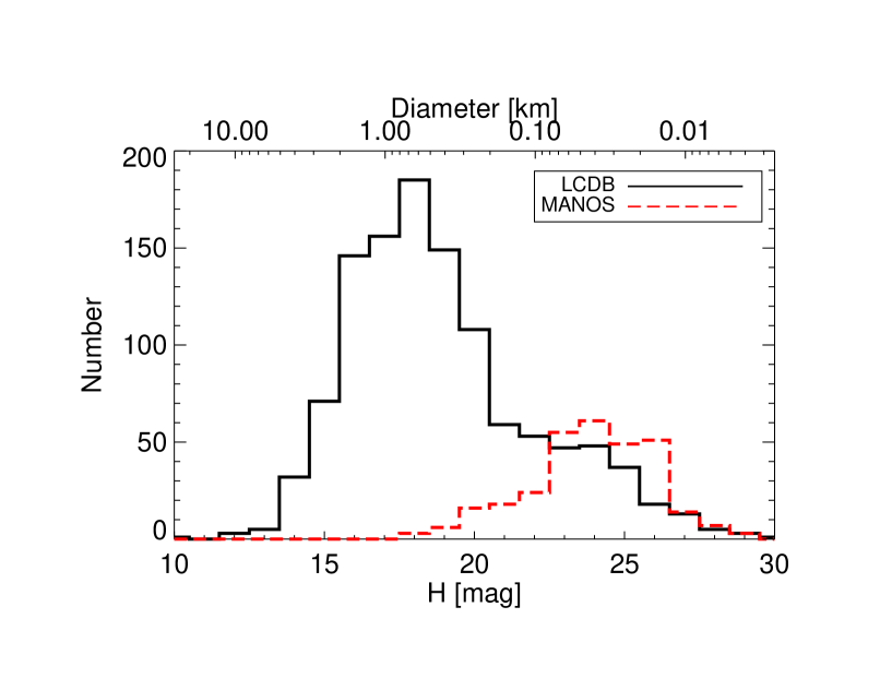
In approximately 4.5 years, MANOS observed 308 NEOs for lightcurves (86 objects in Thirouin et al. (2016), 142 here, and the remainder will be reported in a future work). Figure 1 summarizes the objects observed by MANOS with NEOs from the LCDB¹¹1Lightcurve database (LCDB) from November 2017. (Warner et al., 2009). The LCDB contains 1,359 entries for NEOs, and 1,147 have a rotation estimate (objects with a constraint for the period are not considered). The LCDB distribution peaks at H $\sim$ 17 mag (i.e., NEO with a diameter of D $\sim$ 1 km for a geometric albedo of 20 $\%$ , Pravec & Harris (2007)), whereas for the MANOS sample the peak is at H $\sim$ 24 mag (i.e., D $\sim$ 45 m).

MANOS employs a set of 1 to 4 m telescopes for photometric purposes: 1.3 m Small and Moderate Aperture Research Telescope System (SMARTS) telescope at CTIO, the 2.1 m and the 4 m Mayall telescopes at Kitt Peak Observatory, the 4.1 m Southern Astrophysical Research (SOAR) telescope, and the Lowell’s Observatory 4.3 m Discovery Channel Telescope (DCT). A complete description of these facilities, used instruments and filters is available in Thirouin et al. (2016). In January 2016, Mosaic-1.1 was replaced by Mosaic-3 at the Mayall telescope. This new instrument is also a wide field imager with four 4096 $\times$ 4096 CCDs for a 36 $\arcmin$ $\times$ 36 $\arcmin$ field of view and 0.26 $\arcsec$ /pixel as scale.

Our observing method and data reduction/analysis is summarized in Thirouin et al. (2016). Periodograms are in Appendix A whereas the lightcurves²²2Lightcurves and photometry files can be found at manos.lowell.edu are in Appendix B. Typical photometric error bars are $\pm$ 0.02-0.05 mag, but can be larger in some cases especially with small facilities, faint objects or fast moving objects.

3 MANOS: Photometry summary

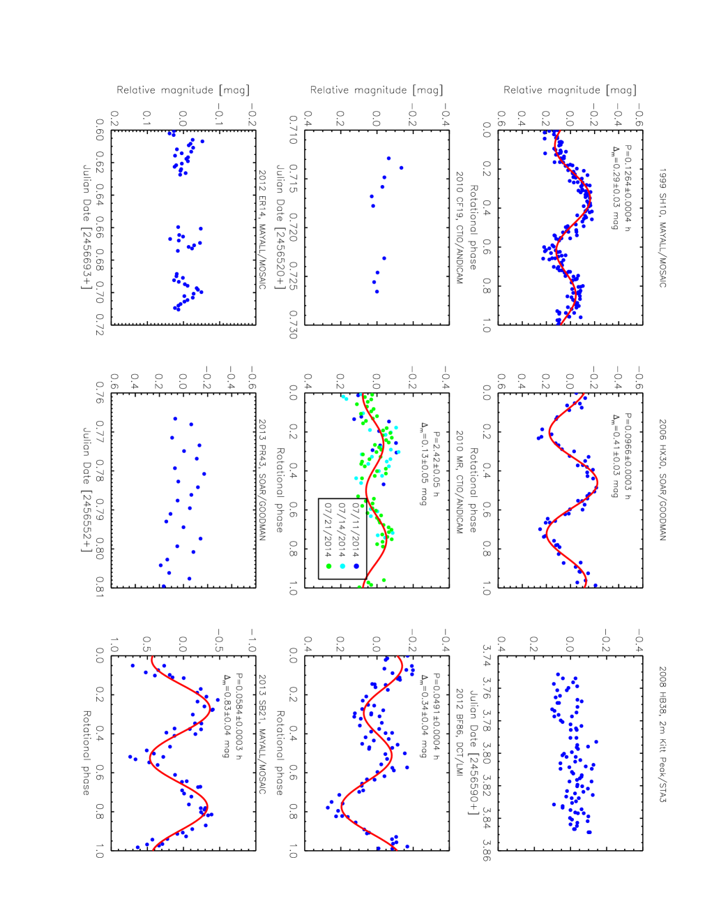
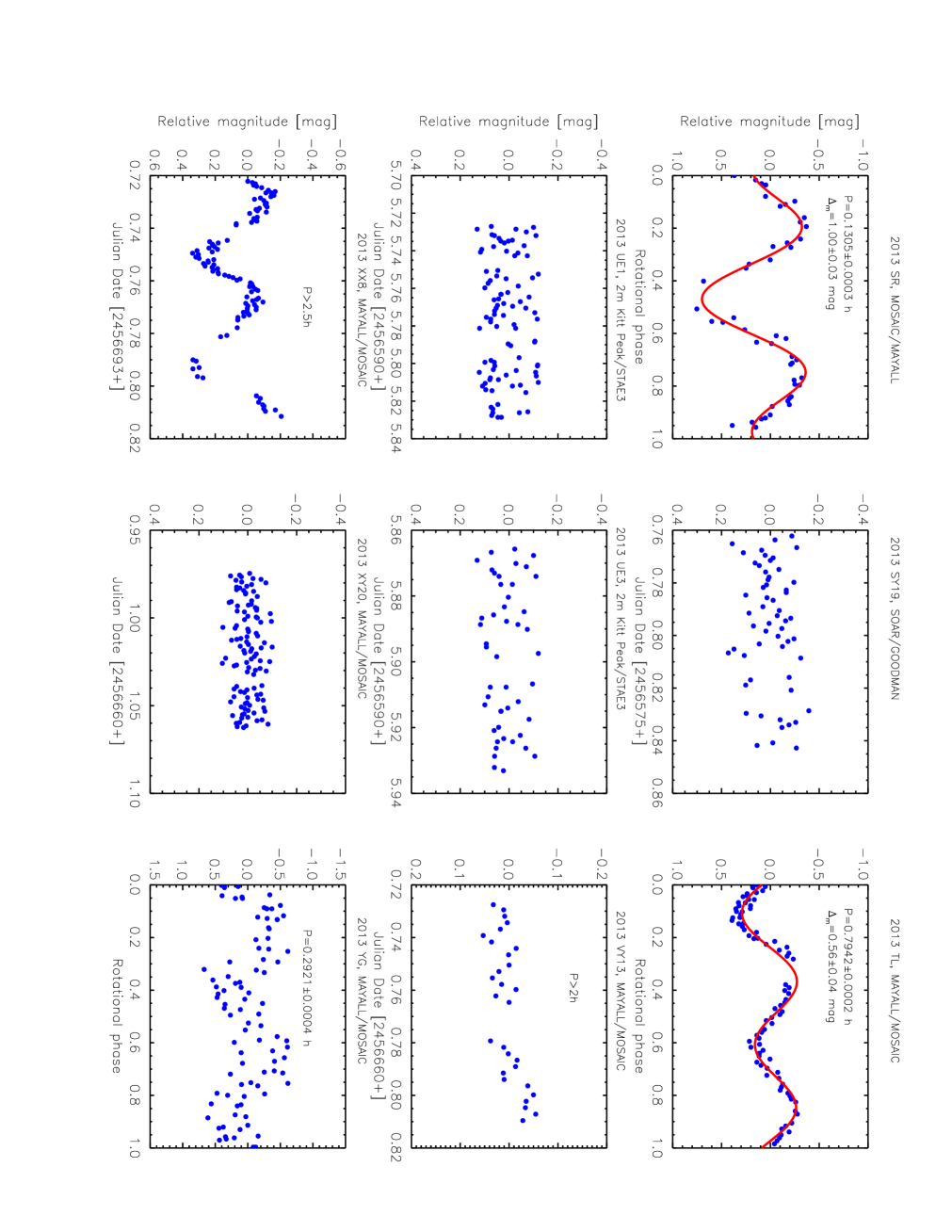
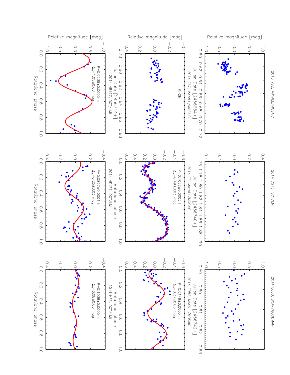
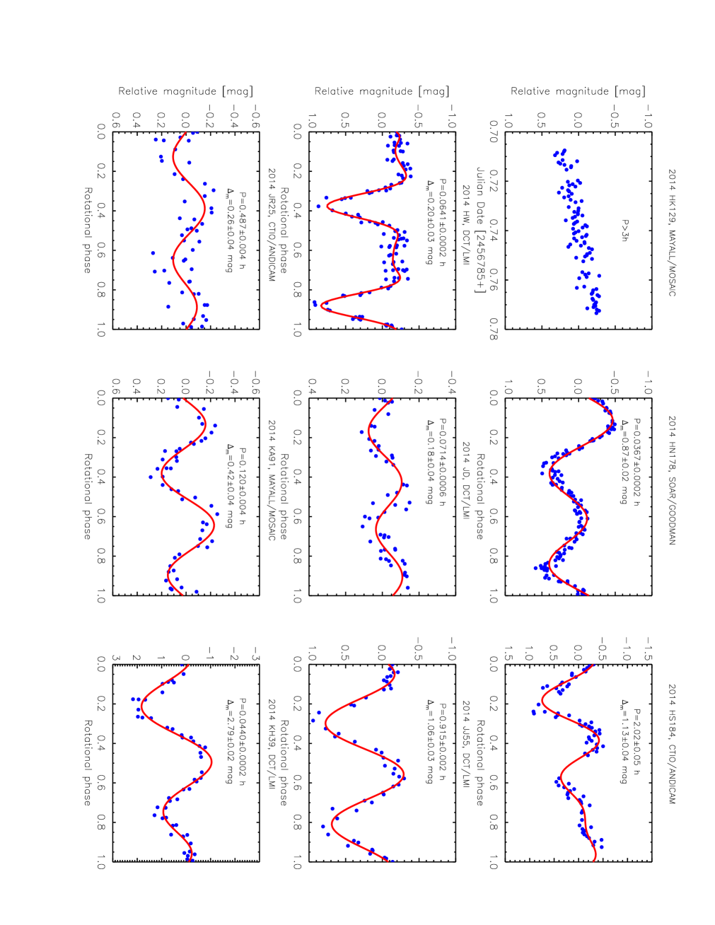
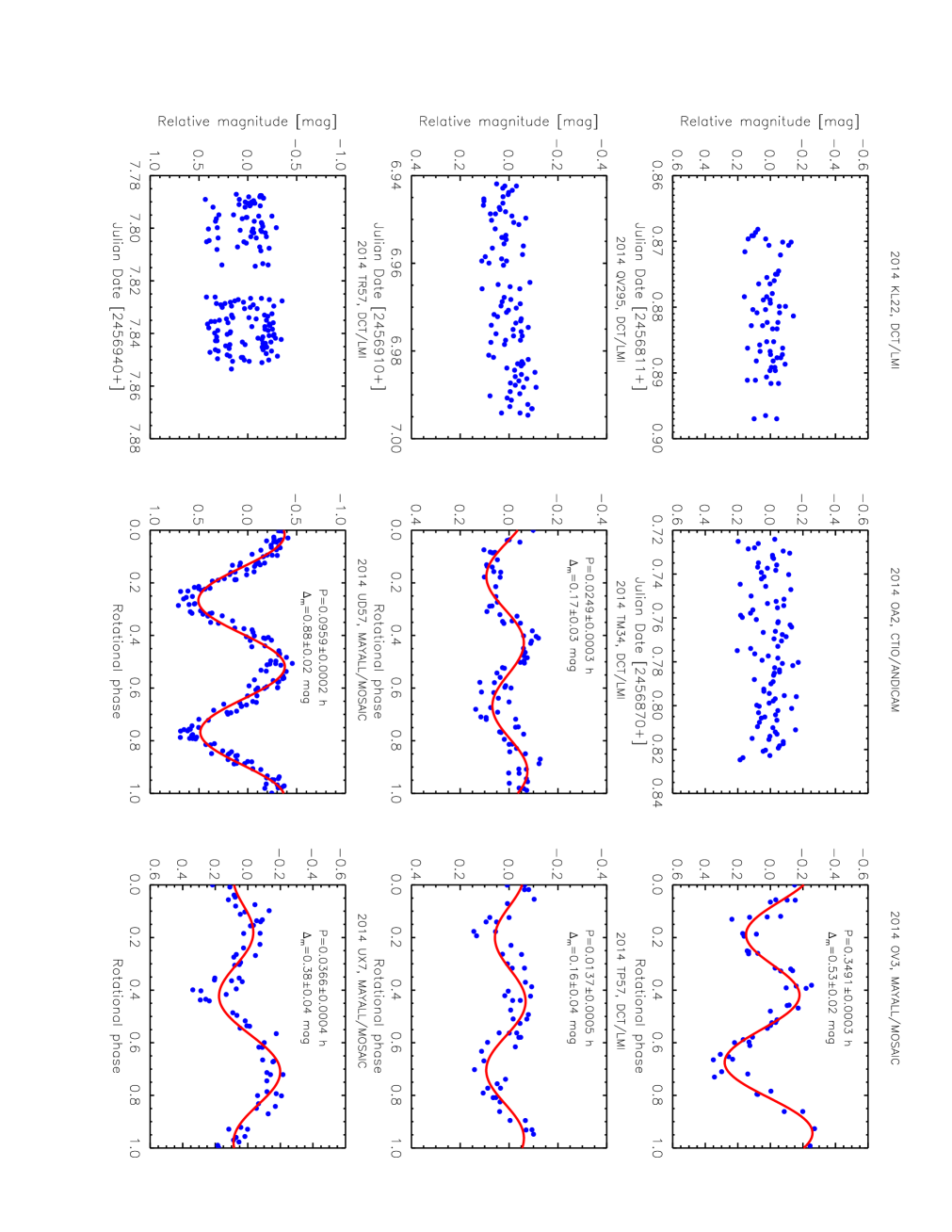
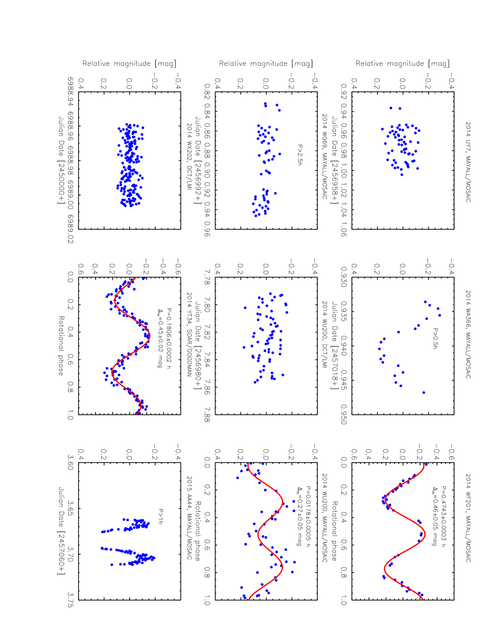
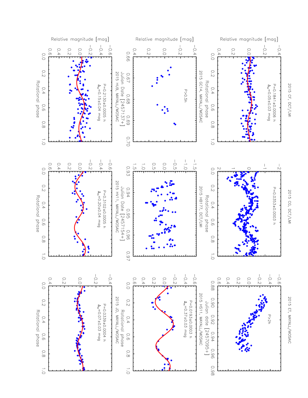
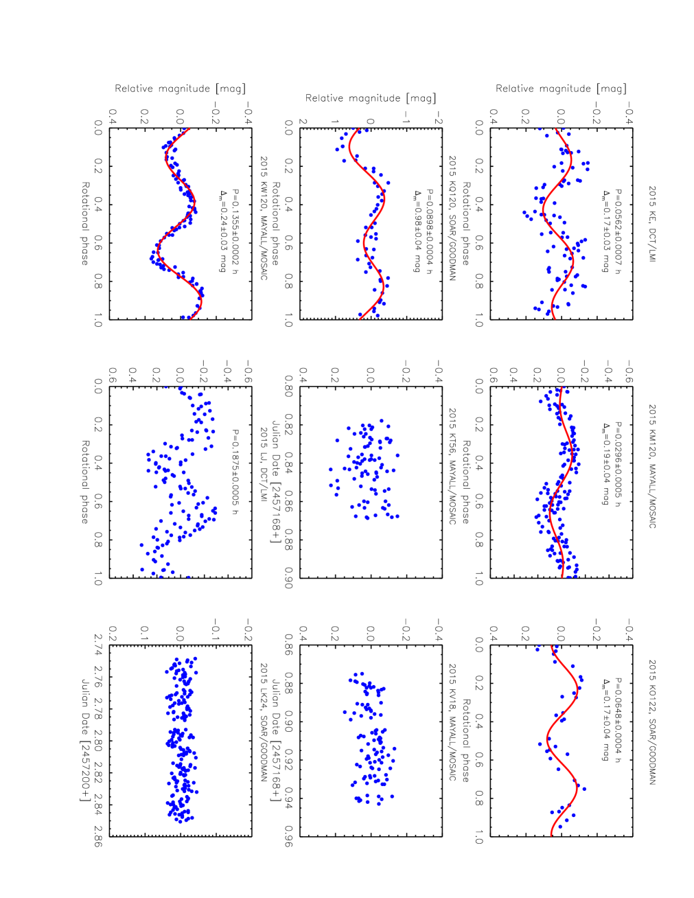
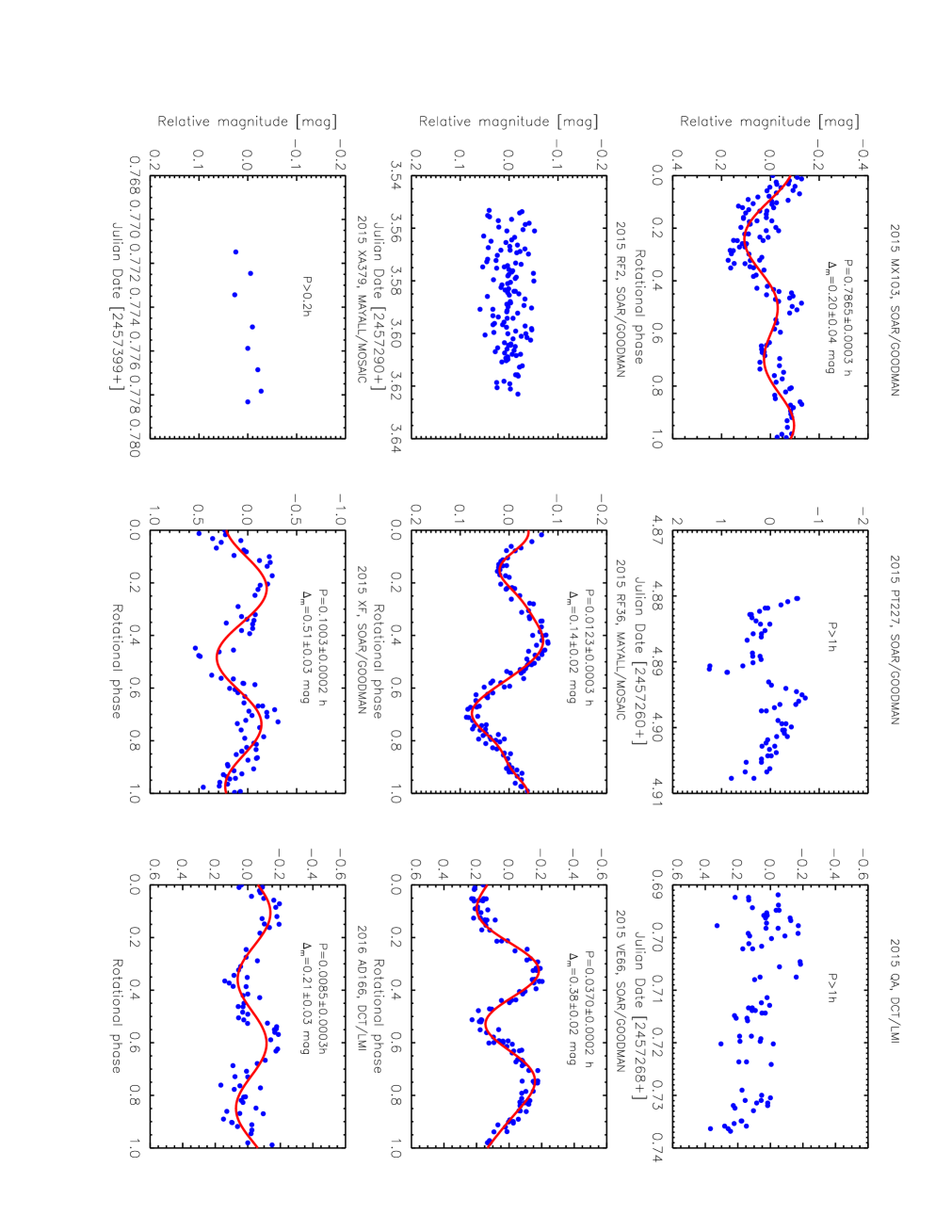
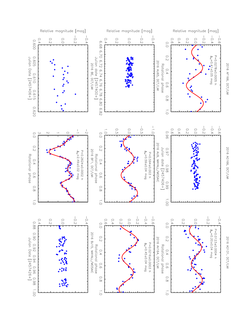
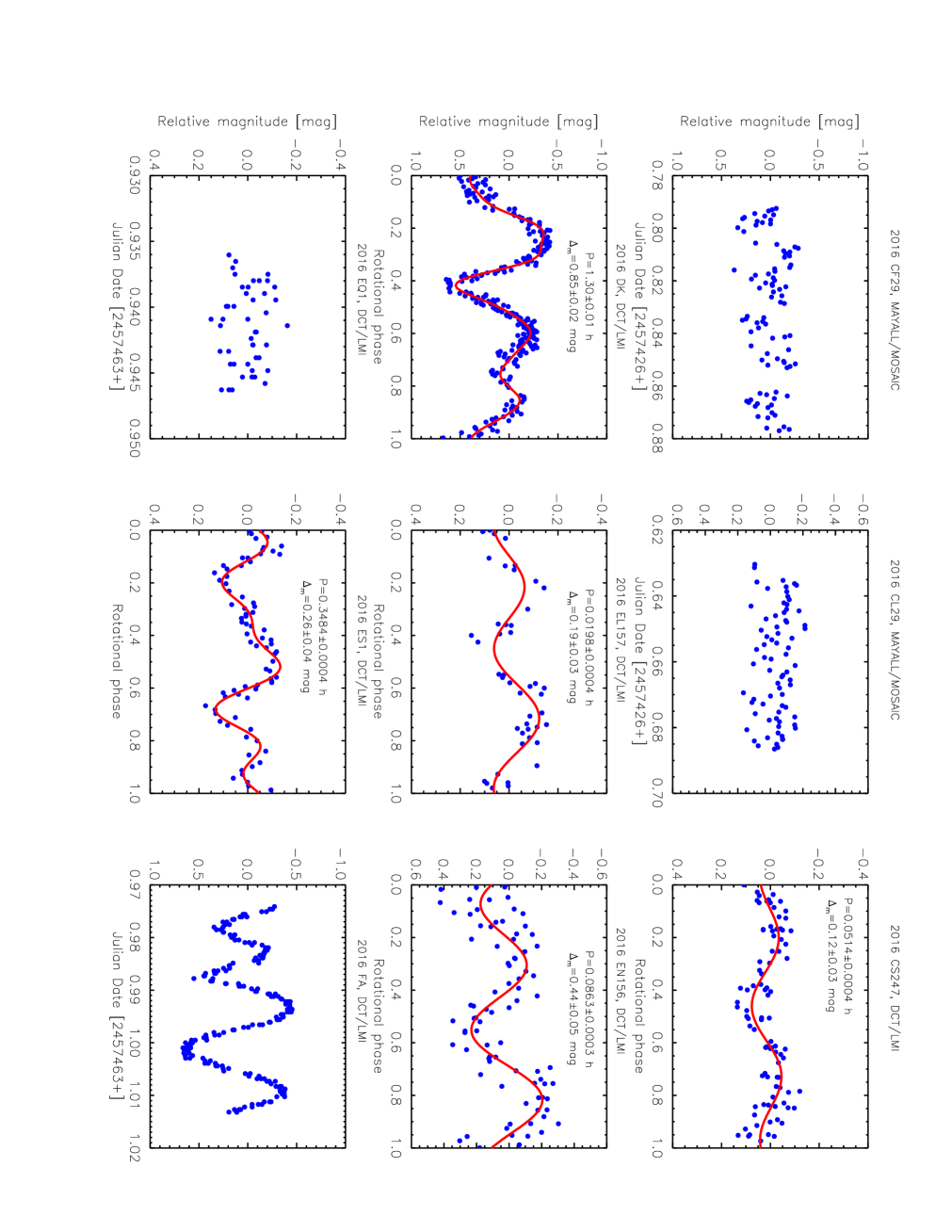
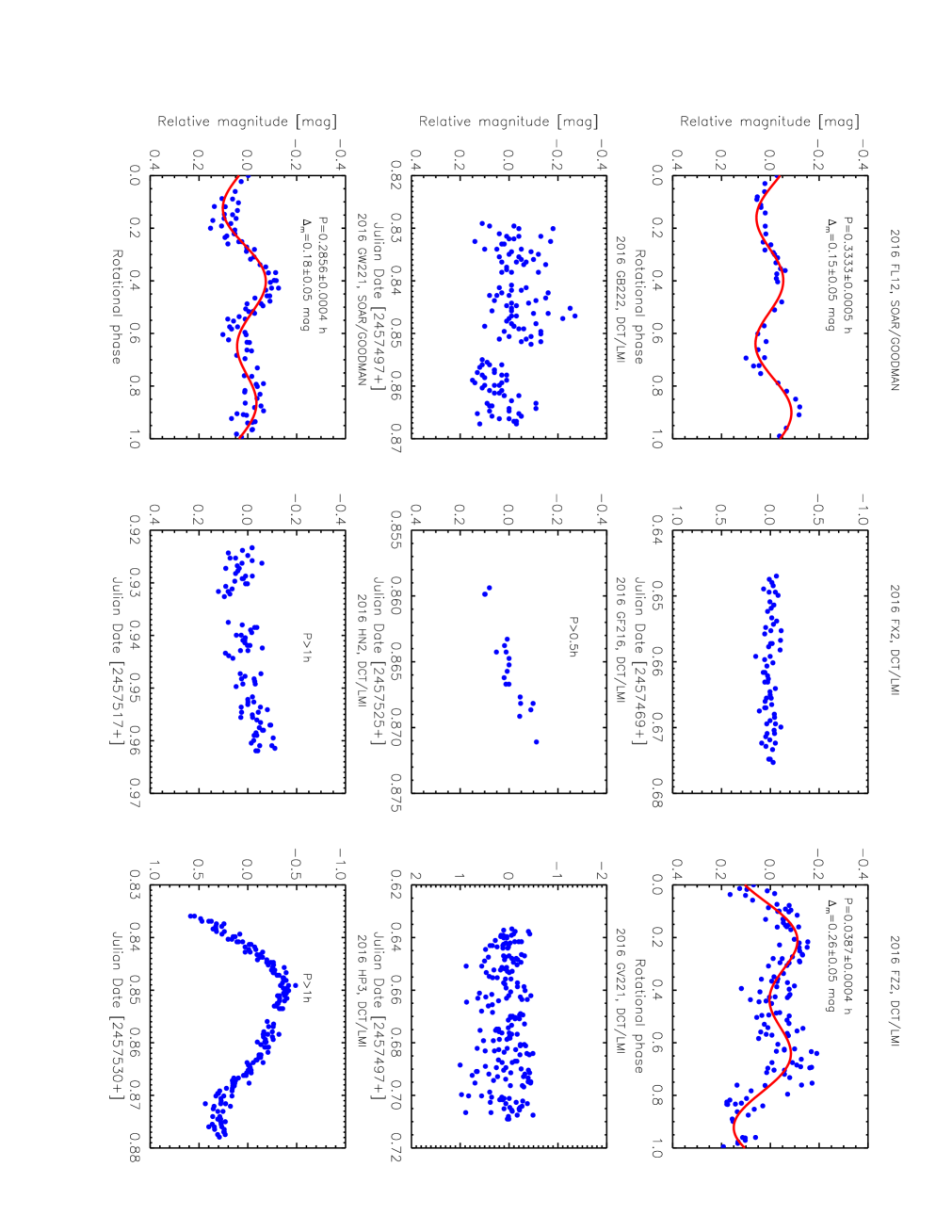
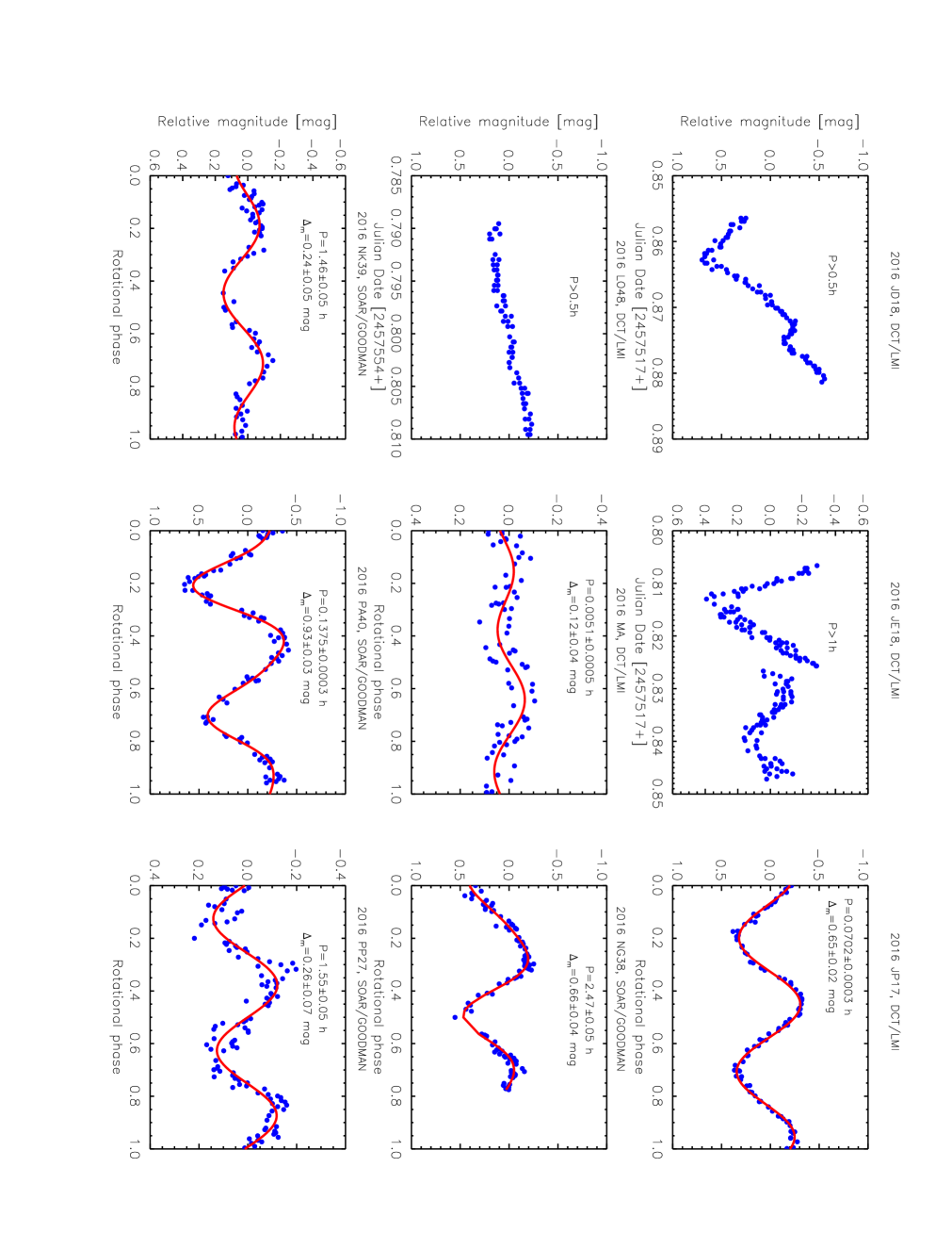
For this work, we classified the lightcurves in four main categories: i) full lightcurve with a minimum of one entire rotation or a large portion of the lightcurve to estimate a periodicity, ii) partial lightcurve showing a decrease or increase of the visual magnitude, but with not enough data for a period estimate, iii) flat lightcurve with no obvious increase/decrease in variability and no period detected, and iv) potential tumblers with or without the primary period (or shortest period, Pravec et al. (2005)). We have full lightcurves for 82 NEOs³³3We have 2 lightcurves for 2014 WU₂₀₀. Only the full lightcurve is considered for these estimates. ( $\sim$ 57 $\%$ of our dataset), lower limits for periodicity and amplitude for 21 NEOs ( $\sim$ 15 $\%$ ), flat lightcurves for 30 NEOs ( $\sim$ 21 $\%$ ), and 10 NEOs are potential tumblers ( $\sim$ 7 $\%$ ) (see Figure 2). We present two lightcurves (one flat and one full) for 2014 WU₂₀₀. This case will be discussed below.

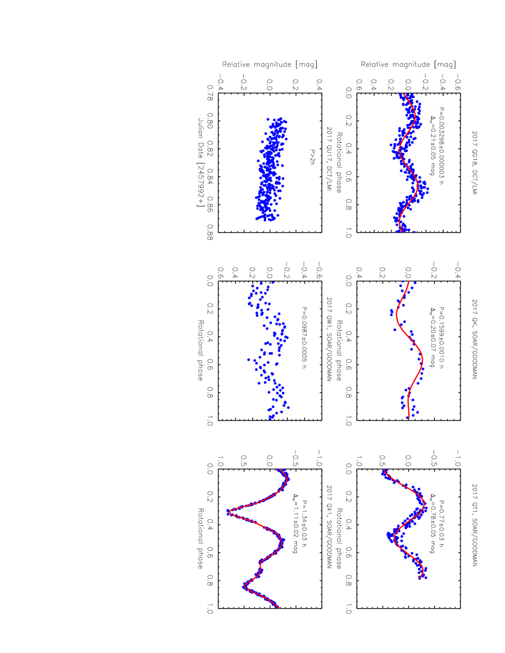
MANOS found the fastest known so far rotator: 2017 QG₁₈ with a rotation of 11.9 s. This object was imaged at DCT in August 2017, and the lightcurve has a variability of about 0.21 mag. The typical photometry error bar is 0.05 mag. We discovered the potential ultra-rapid rotator: 2016 MA. MANOS observed this object in June 2016, and measured a short period of 18.4 s. The typical photometry error bar is 0.05 mag. The lightcurve displays low variability with a full amplitude of 0.12 mag. Unfortunately, the confidence level of this periodicity is low (i.e., $<$ 99.9 $\%$ confidence level stated for a period estimate) and more data are required to infer if 2016 MA is a ultra-rapid rotator or not. In summary, MANOS discovered four ultra-rapid rotators with periodicities below 20 s: 2014 RC, 2015 SV₆, 2016 MA, and 2017 QG₁₈ (Thirouin et al. (2016), and this work).

3.1 Asymmetric/Symmetric and Complex lightcurves

Only three NEOs display a symmetric lightcurve: 2014 UD₅₇, 2014 WF₂₀₁, and 2017 LD, whereas 66 have a bimodal lightcurve with two different peaks ⁴⁴4Tumblers are not considered in this subsection (i.e. asymmetric curve). Majority of the MANOS NEOs has an asymmetry $<$ 0.2 mag, but sometimes, the difference is higher: 2013 SR and 2015 KQ₁₂₀ with an asymmetry of $\sim$ 0.5 mag, 2014 FF with $\sim$ 0.3 mag, 2014 HN₁₇₈ with $\sim$ 0.4 mag, and 2014 KH₃₉ with $\sim$ 0.7 mag.

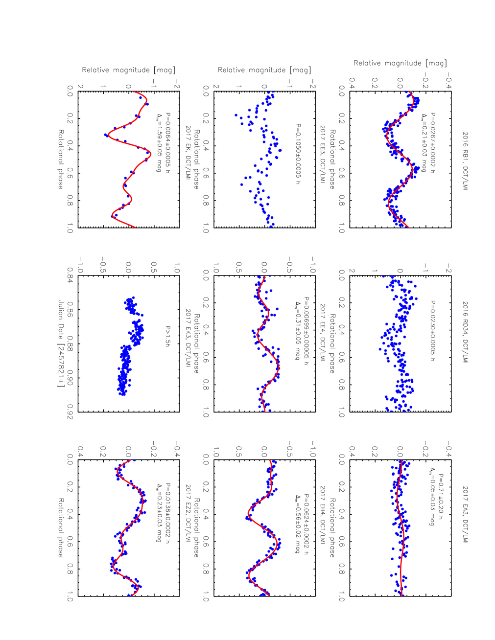
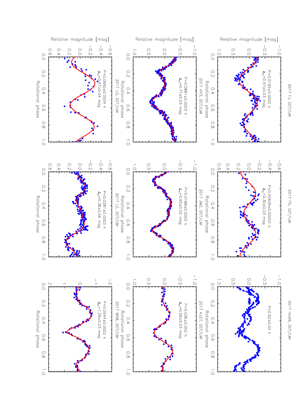
Thirteen objects have complex lightcurves that cannot be fit with only two harmonics: 2014 HS₁₈₄, 2014 HW, 2016 BF₁, 2016 DK, 2016 ES₁, 2017 EK, 2017 EZ₂, 2017 HV₃, 2017 JM₂, 2017 KZ₂₇, 2017 LE, 2017 MO₈, and 2017 QX₁. Reasons fr this morphology are: i) complex shape (NEOs far from spherical/ellipsoidal shapes), and/or ii) albedo contrast, and/or iii) satellite. More observations in different geometries will be useful for shape modeling and to probe for a companion. Unfortunately, most of them won’t be brighter than 21 mag in the upcoming decade.

3.2 Partial lightcurves

Twenty-one objects display an increase/decrease in magnitude (red arrows Figure 2). We did not calculate a secure periodicity because our observations spanned less than 50 $\%$ of the NEO’s rotation. For example, 2016 JD₁₈ was imaged with Lowell’s DCT for a span of $\sim$ 0.5 h. The partial lightcurve presents a large amplitude of $\sim$ 1.2 mag and a feature possibly suggesting a complex shape.

3.3 Tumblers

We found ten potential tumblers: 2013 YG, 2014 DJ₈₀, 2015 CG, 2015 HB₁₇₇, 2015 LJ, 2016 FA, 2016 RD₃₄, 2017 EE₃, 2017 HU₄₉, and 2017 QW₁. We derive their main periodicities and report them in Table 1. For three of them, we are not capable to deduce the main period. In all cases, our data were insufficient to derive the second period with the Pravec et al. (2005) technique.

3.4 Flat lightcurves

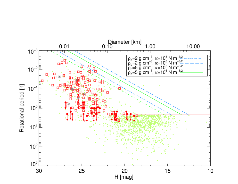
Thirty objects have no detected periodicity in the measured photometry. These flat lightcurves can be due to: i) a long/very long periodicity which was not detected over our observing window , ii) a rapid rotation consistent with the exposing time, iii) a (nearly) pole-on configuration, or iv) a NEO with a spheroidal shape. Below, we discuss these four scenarios by assuming that all small NEOs are fast rotators and large NEOs are slow rotator. Such an assumption is based on the well known rotational period-size relation (Figure 2), but it is important to emphasize that our assumption may not be right for all objects as some small objects have been found to be slow rotators (Warner et al., 2009). Thus, MANOS can be identifying slow or fast rotator in the small size range.

4 Flat lightcurves: Four scenarios

4.1 Slow rotators

As we only dedicate a short observing block per object (typically $\sim$ 2-3 h, or shorter in case of weather or technical issues), we are biased against long rotational periods (typically, longer than 5-6 h). Five objects from this work and Thirouin et al. (2016) were observed by other teams that derived the following rotation periods: 1994 CJ₁ ( $\sim$ 30 h, Warner (2015)), 2008 TZ₃ (44.2 h, Warner et al. (2009)), 2013 YZ₃₇ (8.87 h, Warner (2014)), 2014 SM₁₄₃ (2.9 h, Warner (2015)), and 2015 LK₂₄ (18.55 h, Warner (2015)). For 2014 SM₁₄₃, the Warner (2015) observations and ours are separated by about 8-10 days. In both cases, data were obtained at high phase angle ( $>$ 50^∘). We observed 2014 SM₁₄₃ over $\sim$ 2.5 h with a typical photometric error bar of 0.1 mag and should have detected such a period, assuming that the period derived by Warner (2015) is correct. However, Warner (2015) presented a noisy photometry and their period spectrum showed several solutions that were marginally significant. Therefore, authors not confident about their results, and the reported period could be wrong. Our results about 2014 SM₁₄₃ are available in Thirouin et al. (2016).

We expect “large” objects with D $>$ 100 m (i.e., H $>$ 22.4 mag) to have a slow rotation (Figure 2). Therefore, 2004 BZ₇₄, 2005 RO₃₃, 2007 CN₂₆, 2008 HB₃₈, 2010 CF₁₉, 2011 ST₃₂₃, 2011 WU₉₅, 2012 ER₁₄, 2012 XQ₉₃, 2014 CP₁₃, 2014 OA₂, and 2014 YD₄₂ are probably slow rotators with periods undetected over our short sampling. 2013 UE₃, and 2016 AU₆₅ (H=22.7 mag, and 22.9 mag, respectively) are likely slow rotators too (Figure 2). No other published data on these objects for comparison to our results are published. The length of our observing blocks is the lower limit for their periods.

In conclusion, 19 large objects (D $\gtrsim$ 100 m) in the full MANOS sample are potential slow rotators (i.e,. $\sim$ 8 $\%$ of the full sample reported in Thirouin et al. (2016) and here). Thus, we estimate that at least 43 $\%$ of our flat lightcurves from this work and our previous paper are caused by slow rotation undetectable over our typical observing blocks. It is crucial to mention that for this estimate, we consider that all large objects are slow rotators which may not be the case for all of them.

4.2 Pole-on orientation

Pole orientations are known for a handful of large NEOs with diameters of several km (e.g., La Spina et al. (2004); Vokrouhlický et al. (2015); Benner et al. (2015)). Shape modeling with radar observations and/or lightcurves obtained at different epochs are required to estimate the pole orientation. MANOS targets typically fade in a matter of hours or days, and their next optical window is often decades away, so lightcurves at different epochs/observing geometries are generally not feasible. For fast and small rotators, radar techniques cannot construct the object’s shape, and thus no pole orientation is derived.

The pole orientation distribution of large objects in the main belt of asteroids (MBAs) is isotropic whereas small MBAs and NEOs (D $<$ 30 km) have preferentially retrograde/prograde rotation (Vokrouhlický et al., 2015; Hanuš et al., 2013; La Spina et al., 2004). Vokrouhlický et al. (2015) report 38 pole solutions with an excess of retrograde-rotating NEOs, and noticed a clear deficit of small MBAs and NEOs with a pole orientation of 0^∘. The MANOS set is mostly composed of NEOs in the sub-100m range, and unfortunately, there is no comprehensive information about pole-orientation for this size-range. However, if the sub-100m NEOs follow the same trend as small main belt asteroids and large NEOs, then we expect an excess of small bodies with a pole orientation of $\sim$ $\pm$ 90^∘.

If the rotation axis of an elongated NEO and the sight line are (nearly-) aligned, the brightness variation due to its rotation will be undetectable. Depending of the aspect angle ( $\theta$ ), the lightcurve amplitude of an elongated object (a $>$ b $>$ c) is:

\Delta m=2.5\log\sqrt{\frac{\bar{a}^{2}\cos^{2}\theta+\bar{a}^{2}\bar{c}^{2}\sin^{2}\theta}{\bar{a}^{2}\cos^{2}\theta+\bar{c}^{2}\sin^{2}\theta}}

(1)

where $\bar{a}$ =a/b, $\bar{b}$ =1, and $\bar{c}$ =c/b. The likelihood to observe an object pole-on is P = 1- $\cos$ $\theta$ (Lacerda & Luu (2003)). As an example, the probability of viewing a small body with a pole-on orientation $\pm$ 5^∘ is $<$ 1 $\%$ . Therefore, we estimate that only a few if any of our flat lightcurves are due to a pole-on orientation.

4.3 Spherical objects

Using the previous equation, the largest amplitude will be at $\theta$ =90^∘, and the smallest at $\theta$ =0^∘ and 180^∘. At $\theta$ =90^∘, $\Delta$ m=2.5 $\log$ ( $\bar{a}$ ). Therefore, the brightness variability of an almost spherical object will be flat. As said, shape modeling using radar observations and/or lightcurves at different epochs are required to derive the object’s shape. However, there are very few shape models available for sub-100m NEO (Benner et al., 2015).

Several NEOs with D $>$ 200 m have an oblate shape with ridge at the equator or a diamond shape, and they are predicted to be relatively common (Benner et al., 2015). Objects like Bennu, 2008 EV₅, 2004 DC, 1999 KW₄, and 1994 CC have an oblate shape based on radar observations, and a low to moderate lightcurve amplitude with periods longer than 2 h (Pravec et al., 2006; Ostro et al., 2006; Warner et al., 2009; Taylor, 2009; Brozović et al., 2011; Busch et al., 2011; Nolan et al., 2013; Benner et al., 2015). Assuming that small NEOs are following the same tendency as NEOs with D $>$ 200 m, some MANOS NEOs are potentially oblate. Oblate objects appear to have long rotational periods that are consistent with/longer than the length of our runs. Therefore, some of our flat lightcurves are potentially caused by oblate objects. Unfortunately, as there is no estimate for the quantity of oblate rotators (independent of size) or if small NEOs have the tendency to be oblate, we cannot propose a clear percentage.

4.4 Fast rotators

The periodicities of small NEOs (D $<$ 100m) may be undetected as a result of “long” exposure times. For example, we report two lightcurves for 2014 WU₂₀₀. One of the lightcurves is flat, but the second displays periodic photometric variations. The first lightcurve was obtained on November 26^th 2014 at DCT. The visual magnitude of 2014 WU₂₀₀ was 20.7 mag (MPC estimate). Due to the faintness and bad atmospheric conditions, we selected an exposing time of 45-55 s (+read-out of 13 s). The typical photometry error bar was 0.03 mag for the DCT data. We re-observed with the Mayall telescope this object few days later when the magnitude was 20.1 mag (MPC estimate). In this case, we employed 10 s as exposure time (+11 s of read-out time), and we favored a rotation of $\sim$ 64 s. The typical photometry error bar was 0.05 mag for the Mayall data. Therefore, the exposing time used at DCT was too long to derive such a short period.

Some of our objects with flat lightcurves were imaged with exposing times between 30 s to 300 s. These values were selected for a decent signal to noise, but these times may not have been optimal to sample the lightcurve and so no periodic photometric variations were detected. We estimate that 23 MANOS NEOs are maybe fast to ultra-rapid rotators whose rotation was undetected due to a “long” exposing time and/or the bad weather conditions⁵⁵5Only objects observed with our 4-m class facilities are considered as most of our data are from 4-m class telescopes.. Small NEOs are commonly rotating fast (Figure 2), and if so, 52 $\%$ of our flat lightcurves from this work and Thirouin et al. (2016) are potentially due to small ultra-rapid/fast rotators.

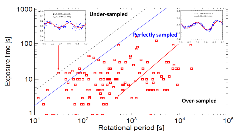
For fast/ultra-rapid NEOs rotating in few seconds or few minutes, the exposure time is important. Following Pravec et al. (2000), the optimum exposure time (T ${}_{exp}^{opt}$ ) to detect a lightcurve with two harmonics is:

T_{exp}^{opt}=0.185\times P

(2)

with P as the object’s periodicity (Section 2 of Pravec et al. (2000)). This relation is based on theory and does not reflect a specific observing strategy. Because we know the exposing time during our observations, we can figure out the detectable rotational period. For example, with T_exp=11 s, we will perfectly sample the lightcurve of a small body rotating in 1 min or more. In this case, an object rotating in $\ll$ 1 min will have a flat lightcurve and thus its rotation will be undetectable.

In Figure 3, the continuous line is for Equation 2 for a perfectly sampled two harmonic lightcurve. Data points are MANOS NEOs imaged with our 4-m facilities. Objects below the continuous line have over-sampled lightcurves whereas above this line the lightcurves are under-sampled. The dash line in Figure 3 represents an empirical upper limit to the period-exposure time relationship using the MANOS dataset and can be articulated as:

T_{exp}^{MANOS}=0.48\times P

(3)

This relation would converge to Nyquist sampling theory in a regime of infinite signal-to-noise-ratio. For the smallest objects, and thus potentially fast to ultra-rapid rotators, using Equation 3 we can identify the rotational period to which we were sensitive based on object-specific exposure time. Using Equation 2, and Equation 3, we have two lower limits for the potential rotational periods.Therefore, if these objects have a rotational period between these two estimates, we should have detected it. In conclusion, the rotational period is likely shorter than the estimate and thus we undetected it in our observing block (assuming that the objects have a two harmonics lightcurve). But, it is also important to emphasize that some small objects (sub-100m objects), even if they are expected to rotate fast, some might be slow rotators (Figure 2).

5 Physical Constraints

A strenghtless rubble-pile will not be able to rotate faster than about 2.2 h without breaking up (Pravec et al., 2002). But, most small NEOs have rotational periods of a few seconds or minutes. Therefore, an explanation of these rapid rotations is that NEOs are bound with tensile strength and/or cohesive instead of just gravity. Using Holsapple (2004, 2007), we calculated the maximum spin limits assuming different densities and tensile strength coefficients for the NEO population. Following Richardson et al. (2005), we considered a friction angle of 40^∘, and moderately elongated ellipsoids (c/a=b/a=0.7). We used two values for the density; 2 (Itokawa (Fujiwara et al., 2006)) and 5 g cm^-3 (density of a stony-iron object (Carry, 2012)), and two tensile strength coefficients, 10⁵, and 10⁶ N m^-3/2 (range of tensile strengths for Almahata Sitta, Kwiatkowski et al. (2010)). Five MANOS targets require a tensile strength coefficient between 10⁵-10⁶ N m^-3/2: 2014 FR₅₂, 2014 PR₆₂, 2015 RF₃₆, 2016 AD₁₆₆, and 2016 AO₁₃₁.

The lightcurve amplitudes ( $\Delta m(\alpha)$ ) in Table 1 were obtained at a phase angle, $\alpha$ . At $\alpha$ =0^∘, the amplitude is:

\Delta m(\alpha=0^{\circ})=\frac{\Delta m(\alpha)}{1+s\alpha}

(4)

with s=0.03 mag deg^-1 (Zappala et al., 1990). In the MANOS sample, only 12 objects (10 $\%$ of our sample) have a $\Delta m(\alpha=0^{\circ})$ $\geq$ 0.5 mag, and one object has a $\Delta m(\alpha=0^{\circ})$ $\geq$ 1 mag. In the LCDB, there are 309 NEOs⁶⁶6Observing circumstances or lightcurve amplitude are not reported for some LCDB objects, and thus they are not considered here. Only NEOs with a H $\geq$ 20 mag are considered because MANOS focuses on small objects. We select objects observed at a phase angle lower than 100^∘ because MANOS is observing in that range. with an absolute magnitude H $\geq$ 20 mag, and observed at a phase angle $\alpha$ $\leq$ 100^∘: 47 of them have a $\Delta m(\alpha=0^{\circ})$ $\geq$ 0.5 mag (15 $\%$ of the LCDB), and 6 have a $\Delta m(\alpha=0^{\circ})$ $\geq$ 1 mag (2 $\%$ ). Therefore, the relative abundance of high amplitude lightcurves in these two data sets are consistent.

6 Potential mission targets

One of our goals is to find favorable target(s) for a future mission to a NEO, and thus mission accessibility is one of our selection criteria (Abell et al., 2009; Hestroffer et al., 2017; Bambach et al., 2018). For this purpose, we estimate the velocity change for a Hohmann transfer orbit also known as $\Delta v$ . A rough guess of the $\Delta v$ is estimated with the Shoemaker & Helin (1978) protocol ( $\Delta v$ ^SH). In order to obtain an accurate estimate, one can use the Near-Earth Object Human Space Flight Accessible Targets Study (NHATS) orbital integration, $\Delta v$ ^NHATS ⁷⁷7http://neo.jpl.nasa.gov/nhats/. NHATS uses specific constraints to compute the $\Delta v$ ^NHATS: i) Launch before 2040, ii) Total mission duration $\leq$ 450 days, and iii) Number of days spent at the object $\geq$ 8 days. The NHATS limit is $\Delta v$ ^NHATS of 12 km s^-1. Several of our targets are not following these criteria and so, no $\Delta v$ ^NHATS are available for them (Table 1).

According to NHATS, 78 MANOS NEOs are accessible by a spacecraft (Table 2, and Table 2 in Thirouin et al. (2016)). For diverse reasons, Abell et al. (2009) consider that the best target for a mission should have a moderate to slow rotation (P $>$ 1 h). Only 9 MANOS NEOs have such a long rotation, have a $\Delta v$ ^NHATS $\leq$ 12 km s^-1; and have been observed for spectroscopy (Table 2, and Table 2 in Thirouin et al. (2016)). We will present spectral results for these objects in future publication(s).

Finally, we note that several non-fully characterized MANOS NEOs have a new optical window in the upcoming years or decades. For example, the low $\Delta v$ ^NHATS and slow rotator 2013 XX₈ (spectral type unknown) will have a new optical window in 04/2019 and thus we will have an opportunity to fully characterize this potential target.

7 MANOS+LCDB versus synthetic population

In this section, we aim to compare our results to a synthetic population of NEOs to identify biases regarding our measured amplitude distribution and to constrain the distribution of morphologies in the NEO population. In a first step, we create 10,000 synthetic objects and calculate their lightcurve amplitude versus aspect angle. In a second step, we “observationally sample” this synthetic population based on prescribed phase angles, in order to compare our synthetic population with the MANOS+LCDB data set.

Step 1:

Assuming that NEOs are prolate ellipsoids (with b=c) at a phase angle of 0^∘, the amplitude varies as:

\Delta m(\theta)=1.25\times\log\Big{[}\frac{1}{\cos^{2}\theta+(b/a)^{2}\sin^{2}\theta}\Big{]}

(5)

where $\theta$ is the aspect angle, and b/a is the elongation of the object (Michalowski & Velichko, 1990). The aspect angle is:

\cos\theta=-\sin\beta_{g}\sin\beta_{p}-\cos\beta_{g}\cos\beta_{p}\cos(\lambda_{g}-\lambda_{p})

(6)

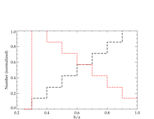
where $\beta_{p}$ and $\lambda_{p}$ are the object’s north pole ecliptic latitude and longitude, and $\lambda_{g}$ and $\beta_{g}$ are the object geocentric ecliptic coordinates (Michalowski & Velichko, 1990). We use Equation 5 to generate the lightcurve amplitude of 10,000 synthetic objects. The only two free parameters in this equation are the axis ratio b/a and the viewing angle $\theta$ . In theory, the axis ratio b/a varies from 0 to 1. However, for objects visited by spacecraft, Eros⁸⁸8Only objects visited by spacecraft were taken into account because of the direct estimate of their size/axis ratio. is the most elongated with a ratio b/a=0.32 (Veverka et al., 2000). Thus, we limit the axis ratio b/a between 0.32 and 1 (spherical object). We considered three possible axis distributions for our synthetic population: i) a uniform distribution of b/a, ii) one distribution with an excess of spheroidal objects and iii) one with an excess of elongated objects (Figure 5, upper panel).

The second parameter is the aspect angle $\theta$ ranging from from 0^∘ to 90^∘ (absolute value). La Spina et al. (2004); Vokrouhlický et al. (2015) noticed an excess of retrograde-rotating NEOs (based on a limited sample) which would imply that the observed distribution of pole orientations is not uniform. We updated the distribution of poles reported in Vokrouhlický et al. (2015) with newest results from the LCDB (multiple systems have been excluded from the distribution as we do not expect any small NEO as binary/multiple, Margot et al. (2002)). With the newest results, the pole distribution is still consistent with the Vokrouhlický et al. (2015) result. Using our updated pole distribution, we created a non-uniform distribution of pole orientation and thus a distribution of ( $\lambda_{p}$ ; $\beta_{p}$ ). Even though most of the objects with a known pole orientation are large objects, and we assume that the pole orientation of the small objects is similar that of large objects. This assumption might be wrong and will need to be tested once more pole orientations of small objects are known. The typical uncertainty on pole orientation is about $\pm$ 10^∘ based on radar and lightcurve inversion results, so we estimated the number of objects within a grid of 10^∘ $\times$ 10^∘. We use the number density of objects in this grid of pole coordinates to randomly assign a pole orientation to each of our 10,000 synthetic objects.

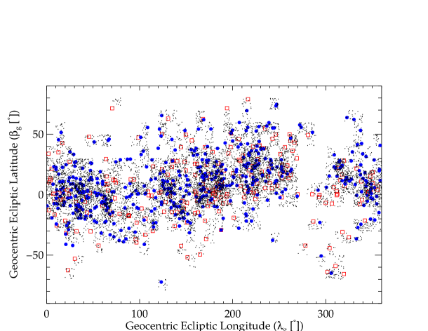
Equation 6 also depends on the geocentric ecliptic coordinates ( $\lambda_{g}$ ; $\beta_{g}$ ). For the MANOS sample, we use the zero phase of our lightcurve to estimate the ( $\lambda_{g}$ ; $\beta_{g}$ ) of our objects. In order to present the most accurate sample, we also incorporated the LCDB objects with H $>$ 20 mag. Unfortunately, authors generally did not report the zero phase timing of their lightcurves. So, we used approximate coordinates for those objects based on the observing nights reported in the literature. Once ( $\lambda_{g}$ ; $\beta_{g}$ ) are estimated for the MANOS+LCDB sample, we created a grid of geocentric ecliptic coordinates of 10^∘ $\times$ 10^∘. Such a grid allowed us to take into account the approximate coordinates of the LCDB objects⁹⁹9In case of observations during close approach, some objects may move more than 10^∘ $\times$ 10^∘ and thus are not in the right grid, however it is a small number of objects and this will not change the main conclusion of our simulations.. Therefore, we created a distribution of ( $\lambda_{g}$ ; $\beta_{g}$ ) based on the observations from the MANOS+LCDB sample (Figure 4, upper plot). Using this and the distribution of ( $\lambda_{p}$ ; $\beta_{p}$ ), we calculated the distribution of aspect angles (Equation 6) which is then used as input to Equation 5 to calculate a synthetic population of lightcurve amplitudes at zero phase.

Step 2:

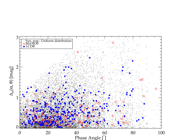
As the aspect angles of our observed sample are unknown, we cannot compare directly our dataset and the synthetic population. However, we can effectively observe our synthetic objects by assigning a phase angle based on the observed distribution of phase angles for MANOS+LCDB objects. By merging Equation 4 and Equation 5, we estimate the lightcurve amplitude of our synthetic population at these prescribed phase angles. In Figure 4, we plot the MANOS sample and the LCDB objects with a H $>$ 20 mag and a phase angle lower than 100^∘. We limit this analysis to small objects observed at a phase angle between 0 and 100^∘ in order to mimic the MANOS sample. Based on Figure 4 (lower plot), it is obvious that the MANOS and LCDB observations are not uniform with phase angle. In fact, both data sets have an excess of objects observed at low/moderate phase angle (up to $\sim$ 40^∘), and only an handful of objects are observed at high phase angle ( $\alpha$ $>$ 80^∘). Drawing from the distribution of MANOS+LCDB objects, we create a non-uniform distribution of phase angles for our synthetic population (Figure 4, lower panel), and then calculate the amplitude of our 10,000 synthetic objects.

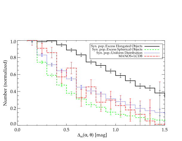
In Figure 5 (lower panel), we plot the normalized histogram of lightcurve amplitude for the synthetic population and the MANOS+LCDB samples. Error bars are $\sqrt{1/N}$ with N being the number of objects per bin. We limit our distribution to lightcurve amplitude up to 1.5 mag as only a handful of objects with higher lightcurve amplitude are reported. Generally, low lightcurve amplitude objects are difficult to obtain as they require a large amount of observing time under good weather conditions. In addition, observers have the tendency to not report or publish flat lightcurves. Therefore, there is a clear bias in the LCDB regarding these low amplitude objects, and thus we do not take into account objects with a lightcurve amplitude $<$ 0.1 mag.

In Figure 5 (lower panel), we plot our three synthetic populations (uniform distribution of b/a, an excess of spherical objects and an excess of elongated objects) for amplitudes between 0.1 mag and 1.5 mag. In order to compare the simulated population and the observed sample, we calculate the $\chi^{2}$ per degree of freedom:

\frac{\chi^{2}}{\nu}=\frac{1}{\nu}\sum_{i}^{n}\Big{[}\frac{f(\Delta m_{i})-\Delta m_{i}}{\sigma_{i}}\Big{]}^{2}

(7)

where $\nu$ is the degree of freedom, $\Delta m_{i}$ are the observed data, f( $\Delta$ m_i) are the simulated results, and $\sigma_{i}$ are the uncertainties (i is the index of the bin and n is the bin number). Comparing the MANOS+LCDB data with the excess of elongated object distribution, we find a $\chi^{2}/\nu$ of 2.67. The MANOS+LCDB sample compared to the excess of spherical object distribution gives us a $\chi^{2}/\nu$ of 1.17, whereas compared to the uniform distribution the $\chi^{2}/\nu$ is 0.31. This suggests that a uniform distribution of b/a best fits the observed sample. Our model assumes a basic uniform distribution of b/a for prolate ellipsoids. Future improvements to this model could employ more realistic shapes based on radar observations and/or lightcurve inversion.

8 Summary/Conclusions

We report full lightcurves for 57 $\%$ of our sample (82 NEOs), and constraints for the amplitude and period are reported for 21 NEOs. Thirty NEOs do not exhibit any periodic variability in their lightcurves. We also report 10 potential tumblers.

MANOS found a potential new ultra-rapid rotator: 2016 MA. This object has a potential periodicity of 18.4 s. The confidence level of this periodicity is low and more data are required to confirm this result. Unfortunately, there is no optical window to re-observe this object until 2025, and even then it only reaches V $\sim$ 22.5 mag. We also uncovered the fastest rotator to date, 2017 QG₁₈ rotating in 11.9 s.

Several MANOS targets display a flat lightcurve. Because of the well known relation between size and rotational period, we can infer that large objects (D $>$ 100 m) are slow rotators and their rotational periods were undetected during the amount of observing time dedicated. Based on this size dependent cut, we estimate that 43 $\%$ of our flat lightcurves are slow rotators with a rotational period longer than our observing blocks. A flat lightcurve of a small NEO can be attributed to fast/ulra-rapid rotation which goes undetected because of the long exposing time used to retrieve a good signal-to-noise ratio. We suggest that 52 $\%$ of our flat lightcures are potential fast/ultra-rapid rotators. We use the size of the object as a main criteria for these findings. This is an acceptable approximation, but may not be true for all the objects.

We present a simple model to constrain the lightcurve amplitude distribution within the NEO population. One of the main parameters of our model is the b/a axis ratio of an object. We create several axis distributions, using an uniform distribution as well as an excess of spherical and elongated objects. Assuming that the pole orientation distribution reported in Vokrouhlický et al. (2015) is representative of the NEO population, we generate 10,000 synthetic ellipsoids. We inferred that an uniform distribution of b/a best matches the observed sample. This suggests that the number of spherical NEOs is roughly equivalent to the number of highly elongated objects.

A total of 78 MANOS objects are mission accessible according to NHATS which assumes a launch before 2040. However, considering only fully characterized objects, and NEOs rotating in more than 1 h, our sample of viable mission targets is reduced to 9 objects: 2002 DU₃, 2010 AF₃₀, 2013 NJ, 2013 YS₂, 2014 FA₇, 2014 FA₄₄, 2014 YD, 2015 FG₃₆, and 2015 OV. Two of these 9 objects will be bright enough during their next observing windows for new and complementary observations: 2013 YS₃ will have a V $\sim$ 18 mag in December-January 2020, and the visual magnitude of 2002 DU₃ will be 20.6 mag in November 2018.

Authors acknowledge the referee for useful comments to improve this work. Lowell operates the Discovery Channel Telescope (DCT) in partnership with Boston University, the University of Maryland, the University of Toledo, Northern Arizona University and Yale University. Partial support of the DCT was provided by Discovery Communications. LMI was built by Lowell Observatory using funds from the National Science Foundation (AST-1005313). This work is also based on observations obtained at the Southern Astrophysical Research (SOAR) telescope, which is a joint project of the Ministério da Ciência, Tecnologia, e Inovação (MCTI) da República Federativa do Brasil, the U.S. National Optical Astronomy Observatory (NOAO), the University of North Carolina at Chapel Hill (UNC), and Michigan State University (MSU). We also used the 1.3 m SMARTS telescope operated by the SMARTS Consortium. This work is based in part on observations at Kitt Peak National Observatory, National Optical Astronomy Observatory (NOAO Prop. ID:2013B-0270), which is operated by the Association of Universities for Research in Astronomy (AURA) under cooperative agreement with the National Science Foundation. This research has made use of data and/or services provided by the International Astronomical Union’s Minor Planet Center. Authors acknowledge support from NASA NEOO grants NNX14AN82G, and NNX17AH06G. D. Polishook is grateful to the Ministry of Science, Technology and Space of the Israeli government for their Ramon fellowship for post-docs.

References

Abell et al. (2009) Abell, P. A., Korsmeyer, D. J., Landis, R. R., et al. 2009, Meteoritics and Planetary Science, 44, 1825
Bambach et al. (2018) Bambach, P., Deller, J., Vilenius, E., et al. 2018, arXiv:1805.01750
Benner et al. (2015) Benner, L. A. M., Busch, M. W., Giorgini, J. D., Taylor, P. A., & Margot, J.-L. 2015, Asteroids IV, 165
Brozović et al. (2011) Brozović, M., Benner, L. A. M., Taylor, P. A., et al. 2011, Icarus, 216, 241
Busch et al. (2011) Busch, M. W., Ostro, S. J., Benner, L. A. M., et al. 2011, Icarus, 212, 649
Carry (2012) Carry, B. 2012, Planet. Space Sci., 73, 98
Fujiwara et al. (2006) Fujiwara, A., Kawaguchi, J., Yeomans, D. K., et al. 2006, Science, 312, 1330
Hanuš et al. (2013) Hanuš, J., Ďurech, J., Brož, M., et al. 2013, A&A, 551, A67
Hestroffer et al. (2017) Hestroffer, D., Agnan, M., Segret, B., et al. 2017, AGU Fall Meeting Abstracts,
Holsapple (2004) Holsapple, K. A. 2004, Icarus, 172, 272
Holsapple (2007) Holsapple, K. A. 2007, Icarus, 187, 500
Kikwaya Eluo (2018) Kikwaya Eluo, J.-B. 2018, The Vatican Observatory, Castel Gandolfo: 80th Anniversary Celebration, 51, 27
Kwiatkowski et al. (2010) Kwiatkowski, T., Polinska, M., Loaring, N., et al. 2010, A&A, 511, A49
Lacerda & Luu (2003) Lacerda, P., & Luu, J. 2003, Icarus, 161, 174
La Spina et al. (2004) La Spina, A., Paolicchi, P., Kryszczyńska, A., & Pravec, P. 2004, Nature, 428, 400
Li et al. (2015) Li, J.-Y., Helfenstein, P., Buratti, B., Takir, D., & Clark, B. E. 2015, Asteroids IV, 129
Margot et al. (2002) Margot, J. L., Nolan, M. C., Benner, L. A. M., et al. 2002, Science, 296, 1445
Michalowski & Velichko (1990) Michalowski, T., & Velichko, F. P. 1990, Acta Astron., 40, 321
Nolan et al. (2013) Nolan, M. C., Magri, C., Howell, E. S., et al. 2013, Icarus, 226, 629
Ostro et al. (2006) Ostro, S. J., Margot, J.-L., Benner, L. A. M., et al. 2006, Science, 314, 1276
Pravec & Harris (2000) Pravec, P., & Harris, A. W. 2000, Icarus, 148, 12
Pravec et al. (2000) Pravec, P., Hergenrother, C., Whiteley, R., et al. 2000, Icarus, 147, 477
Pravec et al. (2002) Pravec, P., Harris, A. W., & Michalowski, T. 2002, Asteroids III, 113
Pravec et al. (2005) Pravec, P., Harris, A. W., Scheirich, P., et al. 2005, Icarus, 173, 108
Pravec et al. (2006) Pravec, P., Scheirich, P., Kušnirák, P., et al. 2006, Icarus, 181, 63
Pravec & Harris (2007) Pravec, P., & Harris, A. W. 2007, Icarus, 190, 250
Pravec et al. (2008) Pravec, P., Harris, A. W., Vokrouhlický, D., et al. 2008, Icarus, 197, 497
Reddy et al. (2015) Reddy, V., Dunn, T. L., Thomas, C. A., Moskovitz, N. A., & Burbine, T. H. 2015, Asteroids IV, 43
Richardson et al. (2005) Richardson, D. C., Elankumaran, P., & Sanderson, R. E. 2005, Icarus, 173, 349
Shoemaker & Helin (1978) Shoemaker, E. M., & Helin, E. F. 1978, Reports of Planetary Geology Program, 20
Taylor (2009) Taylor, P. A. 2009, Ph.D. Thesis, Cornell University.
Thirouin et al. (2016) Thirouin, A., Moskovitz, N., Binzel, R. P., et al. 2016, AJ, 152, 163
Veverka et al. (2000) Veverka, J., Robinson, M., Thomas, P., et al. 2000, Science, 289, 2088
Vokrouhlický et al. (2015) Vokrouhlický, D., Bottke, W. F., Chesley, S. R., Scheeres, D. J., & Statler, T. S. 2015, Asteroids IV, 509
Warner et al. (2009) Warner, B. D., Harris, A. W., & Pravec, P. 2009, Icarus, 202, 134
Warner (2014) Warner, B. D. 2014, Minor Planet Bulletin, 41, 157
Warner (2015) Warner, B. D. 2015, Minor Planet Bulletin, 42, 41
Warner (2015) Warner, B. D. 2015, Minor Planet Bulletin, 42, 256
Warner (2015) Warner, B. D. 2015, Minor Planet Bulletin, 42, 115
Zappala et al. (1990) Zappala, V., Cellino, A., Barucci, A. M., Fulchignoni, M., & Lupishko, D. F. 1990, A&A, 231, 548

\startlongtable

Table 1: Observing log and results^a.

NEO	UT-Date	Nb_im	r_h	$\Delta$	$\alpha$	Filter	Tel	$\Delta T$	t_exp	Rot. P.	$\Delta$ m	$\varphi_{0}$	H	D	Dyn.	$\Delta$ ${}_{V}^{SH}$	$\Delta$ ${}_{V}^{NHATS}$
			[AU]	[AU]	[^∘]			[min]	[s]	[h]	[mag]	[2450000+]		[m]	class	[km s^-1]	[km s^-1]
Full
lightcurve
Symmetric
2014 UD₅₇	10/28/14	182	1.022	0.028-0.029	9.8-9.6	wh	KP4	153	20	0.0959	0.88 $\pm$ 0.02	6958.62714	25.8	20	Apollo	5.19	11.278
2014 WF₂₀₁^b	12/01/14	44	1.010	0.028	29.4-29.5	wh	KP4	28	10	0.4743	0.46 $\pm$ 0.05	6992.62728	25.6	22	Apollo	5.10	7.094
2017 LD	06/04/17	53	1.022	0.0082	15.9-16.1	VR	DCT	21	3	0.0660	0.47 $\pm$ 0.04	7908.83057	27.5	9	Amor	4.47	8.339
Asymmetric
1999 SH₁₀	03/28/14	178	1.120	0.147-0.146	31.7	wh	KP4	201	35	0.1264	0.29 $\pm$ 0.03	6744.87878	22.6	89	Apollo	5.57	8.634
2006 HX₃₀	05/27/15	73	1.049-1.050	0.040	24.7	r’	SOAR	93	20	0.0966	0.41 $\pm$ 0.03	7169.74255	26.2	17	Amor	4.72	10.456
2010 MR	07/11-14-21/14	126	1.494-1.432	0.478-0.418	2.9-4.9	V	CTIO	67;252;120	60	2.42	0.13 $\pm$ 0.05	6849.80986	18.6	566	Amor	6.80	-
2012 BF₈₆	02/22/16	91	1.043	0.0825	46.7-49.6	VR	DCT	71	15	0.0491	0.34 $\pm$ 0.04	7440.68168	22.6	89	Aten	10.14	-
2013 SB₂₁	10/14/13	64	1.031	0.034	12.4-12.5	wh	KP4	49	35	0.0584	0.83 $\pm$ 0.04	6579.77774	27.0	11	Amor	4.47	8.588
2013 SR	10/14/13	51	1.050	0.070	40.5-40.6	wh	KP4	47	10	0.1305	1.00 $\pm$ 0.03	6579.63927	24.1	44	Amor	5.27	-
2013 TL	10/14/13	89	1.022	0.085	70.7-70.8	wh	KP4	57	5	0.7942	0.56 $\pm$ 0.04	6579.97030	22.2	107	Apollo	5.89	-
2014 FF	03/28/14	161	1.030	0.040	35.9-36.2	wh	KP4	72	8	0.1032	0.49 $\pm$ 0.03	6744.68831	24.2	42	Amor	6.51	-
2014 FR₅₂	04/18/14	85	1.135	0.148-0.147	20.1	wh	KP4	46	15	0.0149	0.37 $\pm$ 0.06	6765.66520	23.9	49	Amor	6.09	-
2014 HB₁₇₇	05/06/14	21	1.009	0.0034	87.1-87.8	VR	DCT	11	10	0.0239	1.05 $\pm$ 0.06	6783.97448	28.1	7	Apollo	4.83	6.752
2014 HE₁₇₇	05/06/14	69	1.056	0.049	17.0-16.9	VR	DCT	55	15	0.0897	0.25 $\pm$ 0.03	6783.65329	25.8	20	Amor	5.89	-
2014 HF₅	05/06/14	37	1.055	0.056	33.7-33.8	VR	DCT	45	20	0.1038	0.08 $\pm$ 0.03	6783.91201	25.3	25	Amor	5.92	-
2014 HN₁₇₈	06/16/14	144	1.032	0.044	67.7-67.9	r’	SOAR	142	10	0.0367	0.87 $\pm$ 0.02	6824.72654	23.5	59	Amor	5.58	-
2014 JD	05/06/14	76	1.037	0.030	20.3-20.5	VR	DCT	52	7	0.0714	0.18 $\pm$ 0.04	6783.74905	26.3	16	Apollo	6.13	-
2014 JJ₅₅	06/03/14	52	1.073	0.086	45.2-45.3	VR	DCT	168	120	0.915	1.06 $\pm$ 0.03	6811.71253	25.3	25	Apollo	4.94	6.380
2014 JR₂₅	05/10-11/14	53	1.048-1.057	0.043-0.052	26.2-25.3	V	CTIO	106;75	45	0.487	0.26 $\pm$ 0.04	6787.73564	23.4	62	Apollo	7.65	-
2014 KA₉₁	06/04/14	64	1.034	0.026	40.9-41.0	wh	KP4	32	6	0.120	0.42 $\pm$ 0.04	6812.65859	25.5	23	Apollo	5.57	11.846
2014 KH₃₉	06/03/14	55	1.016	0.0051-0.0050	65.3-66.5	VR	DCT	50	1	0.0440	2.79 $\pm$ 0.02	6811.66803	26.2	17	Apollo	6.53	-
2014 OV₃	02/10/15	56	1.155	0.171	9.9-10.0	wh	KP4	121	70	0.3491	0.53 $\pm$ 0.02	7063.73463	23.2	68	Apollo	4.73	7.046
2014 TM₃₄	10/17/14	106	1.047	0.053-0.054	18.6-18.7	VR	DCT	57	15	0.0249	0.17 $\pm$ 0.03	6947.88390	25.0	29	Amor	5.58	-
2014 TP₅₇	10/17/14	71	1.024	0.028	15.6-15.5	VR	DCT	29	8	0.0137	0.16 $\pm$ 0.04	6947.64265	26.4	15	Amor	5.18	-
2014 UX₇	10/28/14	85	1.068	0.075	10.5-10.6	wh	KP4	102	45	0.0366	0.38 $\pm$ 0.04	6958.84348	25.6	22	Amor	5.26	7.294
2014 WU₂₀₀^c	12/01/14	60	0.996	0.011	16.1	wh	KP4	41	10	0.0179	0.27 $\pm$ 0.05	6992.72115	29.1	4	Apollo	4.17	4.206
2014 YT₃₄	01/13/15	124	1.012	0.037	38.9-39.5	r’	SOAR	133	5	0.1806	0.45 $\pm$ 0.02	7035.55787	24.7	34	Apollo	5.75	9.089
2015 CF	02/11/15	157	1.069	0.086	15.7-15.8	VR	DCT	56	7	0.1841	0.05 $\pm$ 0.03	7064.87459	23.5	59	Amor	5.99	-
2015 HS₁₁	04/25/15	44	1.029	0.023	4.0-4.1	wh	KP4	44	7	0.0193	0.37 $\pm$ 0.04	7137.73600	27.1	11	Amor	4.29	6.683
2015 HU₉	05/08/15	128	1.099-1.098	0.130-0.129	43.8-44.2	wh	KP4	145	30	0.2130	0.15 $\pm$ 0.04	7150.66205	23.4	62	Apollo	8.24	-
2015 HV₁₁	05/08/15	55	1.072	0.068	22.1-22.0	wh	KP4	61	25	0.3102	0.20 $\pm$ 0.04	7150.89848	24.1	44	Amor	6.12	-
2015 JD	05/08/15	98	1.022	0.016	36.1-35.7	wh	KP4	72	5	0.0339	0.07 $\pm$ 0.03	7150.79977	25.5	23	Apollo	6.00	11.965
2015 KE	05/22/15	100	1.043	0.034	27.4-27.5	VR	DCT	66	5	0.0562	0.17 $\pm$ 0.03	7164.65626	26.4	15	Aten	4.54	4.296
2015 KM₁₂₀	05/26/15	166	1.042	0.050	54-53.9	wh	KP4	110	15	0.0296	0.19 $\pm$ 0.04	7168.66447	24.7	34	Amor	6.62	-
2015 KO₁₂₂	05/27/15	43	1.036-1.037	0.024	14.9-14.8	r’	SOAR	39	10	0.0648	0.17 $\pm$ 0.04	7169.83972	27.0	11	Apollo	6.78	-
2015 KQ₁₂₀	05/27/15	62	1.040	0.029	21.2-21.4	r’	SOAR	58	10	0.0898	0.98 $\pm$ 0.04	7169.87814	26.7	13	Apollo	4.89	10.883
2015 KW₁₂₀	05/26/15	159	1.037	0.024	10.5	wh	KP4	63	3	0.1355	0.24 $\pm$ 0.03	7168.76662	26.0	18	Apollo	6.20	-
2015 MX₁₀₃	06/29/15	129	1.045	0.039	42.2	r’	SOAR	111	8	0.7865	0.20 $\pm$ 0.04	7202.58034	24.4	39	Amor	5.36	-
2015 RF₃₆	09/14/15	146	1.053-1.052	0.057	34.5-34.3	wh	KP4	100	15	0.0123	0.14 $\pm$ 0.02	7279.93330	23.4	62	Aten	5.63	6.312
2015 RQ₃₆	09/14/15	69	1.058	0.058	25.6-25.5	wh	KP4	59	20	0.4812	0.23 $\pm$ 0.04	7279.87219	24.5	37	Apollo	5.13	-
2015 TL₂₃₈	10/24/15	52	1.035	0.042	16.4-16.5	VR	DCT	47	5	0.0713	0.46 $\pm$ 0.04	7319.68601	24.9	31	Apollo	7.43	-
2015 VE₆₆	11/24/15	126	1.005	0.021	32.7-33.3	r’	SOAR	101	2	0.037	0.38 $\pm$ 0.02	7350.71888	24.1	44	Amor	6.03	-
2015 XF	12/29/15	98	1.059	0.078	11.9-12.0	r’	SOAR	88	20	0.1003	0.51 $\pm$ 0.03	7385.75211	24.4	39	Amor	6.90	-
2016 AD₁₆₆	01/19/16	85	1.074	0.101	25.1-25.0	VR	DCT	49	15	0.0085	0.21 $\pm$ 0.03	7406.76968	23.6	56	Apollo	7.13	-
2016 AF₁₆₆	01/19/16	37	0.995	0.027	65.6-65.7	VR	DCT	14	10	0.0278	0.41 $\pm$ 0.05	7406.80902	25.4	24	Apollo	6.30	-
2016 AO₁₃₁	01/19/16	65	1.054	0.093	39.6	VR	DCT	27	10	0.0216	0.45 $\pm$ 0.04	7406.99723	24.1	44	Apollo	4.57	9.651
2016 AU₉	01/12/16	59	1.061	0.079	11.6	wh	KP4	135	30	0.594	0.59 $\pm$ 0.04	7399.87573	25.4	24	Amor	6.03	-
2016 AV₁₆₄	01/19/16	40	1.059	0.078	13.6	VR	DCT	15	10	0.0123	0.20 $\pm$ 0.04	7406.94935	24.9	31	Amor	6.24	-
2016 CS₂₄₇	02/22/16	108	1.019	0.033-0.034	27.2	VR	DCT	42	7	0.0514	0.12 $\pm$ 0.03	7440.85852	25.6	22	Apollo	4.43	8.076
2016 EL₁₅₇	03/16/16	50	1.013	0.018	8.7-8.9	VR	DCT	20	1	0.0198	0.19 $\pm$ 0.03	7463.89240	27.1	11	Apollo	6.36	-
2016 EN₁₅₆	03/16/16	94	1.009	0.014	8.7-8.6	VR	DCT	27	2	0.0863	0.44 $\pm$ 0.05	7463.91622	27.8	8	Apollo	4.98	9.108
2016 FL₁₂	04/07/16	46	1.032	0.032	17.3-17.4	r’	SOAR	47	9	0.3333	0.15 $\pm$ 0.05	7485.71234	26.3	16	Apollo	4.74	8.672
2016 FZ₂	03/22/16	139	1.1053	0.062	23.8-23.7	VR	DCT	49	5	0.0387	0.26 $\pm$ 0.05	7469.96281	24.5	37	Amor	6.62	-
2016 GW₂₂₁	04/19/16	113	1.041	0.043	30.3-30.0	r’	SOAR	98	3	0.2856	0.18 $\pm$ 0.05	7497.85083	24.8	32	Aten	7.43	9.526
2016 JP₁₇	05/09/16	95	1.029	0.032	52.3-52.0	VR	DCT	27	1	0.0702	0.65 $\pm$ 0.02	7517.78384	23.1	71	Apollo	6.17	-
2016 MA	06/17/16	51	1.023	0.012	54.7-54.9	VR	DCT	29	5	0.0051	0.12 $\pm$ 0.04	7556.74356	27.5	9	Apollo	5.39	11.229
2016 NG₃₈	07/18/16	101	1.038	0.034	48-48.3	r’	SOAR	114	7	2.47	0.66 $\pm$ 0.04	7587.85278	25.1	28	Amor	5.98	-
2016 NK₃₉	08/15/16	74	1.070	0.085	45.9-46.1	r’	SOAR	107	30	1.46	0.24 $\pm$ 0.05	7616.49071	23.9	49	Amor	5.77	11.025
2016 PA₄₀	08/16/16	98	1.092	0.082	13.7-13.6	r’	SOAR	77	10	0.1375	0.93 $\pm$ 0.03	7616.86135	24.4	39	Apollo	7.16	11.513
2016 PP₂₇	08/16/16	116	1.080	0.081-0.082	32.7-32.8	r’	SOAR	95	5	1.55	0.26 $\pm$ 0.07	7616.69028	23.6	56	Apollo	7.12	-
2016 RB₁	09/07/16	198	1.009	0.0016-0.0012	30.9-28.5	VR	DCT	153	3	0.0267	0.21 $\pm$ 0.03	7638.82497	28.3	6	Aten	7.49	8.626
2017 EA₃	03/09/17	130	1.042	0.071	44.6-44.5	VR	DCT	65	5	0.71	0.05 $\pm$ 0.03	7821.75821	23.2	68	Apollo	6.72	-
2017 EE₄	03/15/17	106	1.000	0.019	71.6-72.1	VR	DCT	30	1	0.00699	0.31 $\pm$ 0.05	7827.99828	25.0	29	Apollo	6.00	-
2017 EH₄	03/09/17	139	1.056	0.070	25.3-25.2	VR	DCT	55	5	0.0624	0.56 $\pm$ 0.02	7821.69563	24.1	44	Amor	5.67	-
2017 FJ	03/19/17	179	1.009-1.008	0.013	8.0	VR	DCT	49	5	0.0165	0.57 $\pm$ 0.03	7831.88047	28.2	6	Apollo	5.51	11.780
2017 FK	03/19/17	108	1.005	0.085-0.084	17.7-18.1	VR	DCT	27	2	0.00428	0.30 $\pm$ 0.03	7831.72251	27.3	10	Apollo	5.61	9.042
2017 QG₁₈	08/27/17	296	1.032	0.024-0.023	22.0-21.8	VR	DCT	91	3	0.003298	0.21 $\pm$ 0.05	7992.64725	27.0	11	Apollo	5.26	11.411
2017 QK	08/21/17	47	1.151	0.147	17.9	VR	SOAR	57	30	0.1599	0.20 $\pm$ 0.07	7986.54836	23.8	51	Apollo	5.45	-
2017 QT₁	08/21/17	158	1.030	0.020-0.019	19.5-20.1	VR	SOAR	70	10	0.77	0.78 $\pm$ 0.05	7986.69346	26.7	13	Apollo	8.07	-
Complex
2014 HS₁₈₄	06/02/14	89	1.069	0.061-0.060	24.0-24.1	V	CTIO	233	20	2.02	1.13 $\pm$ 0.04	6810.56578	23.3	65	Amor	5.72	-
2014 HW	04/24/14	126	1.014	0.0089-0.0087	15.4	VR	DCT	108	4	0.0641	1.16 $\pm$ 0.03	6771.81914	28.4	6	Apollo	4.54	5.690
2016 BF₁	01/19/16	75	1.010	0.035	41.1-41.0	VR	DCT	54	10	0.2624	2.49 $\pm$ 0.02	7407.02439	25.4	24	Apollo	5.59	-
2016 DK	02/22/16	285	1.048	0.108	54.5-54.6	VR	DCT	131	10	1.30	0.85 $\pm$ 0.02	7440.94528	22.4	98	Amor	11.34	-
2016 ES₁	03/16/16	99	1.089	0.095	9.9	VR	DCT	38	3	0.3484	0.26 $\pm$ 0.04	7463.94721	24.1	44	Amor	6.65	-
2017 EK	03/15/17	35	0.995	0.017	86.5-86.6	VR	DCT	10	1	0.0064	1.59 $\pm$ 0.05	7827.99072	24.1	44	Apollo	7.03	-
2017 EZ₂	03/09/17	118	1.008	0.015	15.8-16.4	VR	DCT	39	3	0.0138	0.23 $\pm$ 0.03	7821.80369	25.1	28	Amor	8.75	-
2017 HV₃	08/27/17	278	1.081	0.102	44.1-43.9	VR	DCT	163	7	0.0881	0.77 $\pm$ 0.03	7992.87174	23.7	54	Amor	4.65	8.359
2017 JM₂	05/14/17	225	1.021	0.015	45.7-46.3	VR	DCT	67	2	0.0188	0.65 $\pm$ 0.02	7887.81127	24.3	41	Apollo	9.05	-
2017 KJ₂₇	05/28/17	76	1.023	0.019	60.4-61.0	VR	DCT	19	2	0.036	0.58 $\pm$ 0.03	7901.94000	25.4	24	Apollo	7.16	-
2017 LE	06/04/17	224	1.031	0.019	33.1-32.7	VR	DCT	77	2	0.0281	0.39 $\pm$ 0.06	7908.85535	26.4	15	Amor	6.22	-
2017 MO₈	07/03/17	108	1.018-1.017	0.011	84.8-85.5	VR	DCT	34	1	0.0544	1.58 $\pm$ 0.03	7937.75364	26.0	18	Apollo	6.52	-
2017 QX₁	08/21/17	283	1.050	0.039	10.8-11.0	VR	SOAR	85	5	1.34	1.11 $\pm$ 0.02	7986.86290	24.8	32	Amor	5.53	-
Partial
lightcurve
2013 VY₁₃	01/03/14	36	1.458	0.519	19.4	wh	KP4	118	180	$>$ 2	$>$ 0.1	6660.72197	21.2	171	Apollo	6.30	-
2013 XX₈	02/05/14	133	1.072	0.087	9.2-9.3	wh	KP4	128	30-45	$>$ 2.5	$>$ 0.6	6693.72231	24.4	39	Amor	4.57	10.364
2013 YS₂	01/27/14	122	1.023	0.057	45.9-45.8	wh	KP4	134	15	$>$ 2	$>$ 1.0	6684.60839	23.3	65	Amor	4.77	10.346
2014 FA₇	03/28/14	73	1.025-1.026	0.030	24.3	wh	KP4	127	60	$>$ 2	$>$ 0.2	6744.78622	26.7	13	Apollo	5.17	7.232
2014 HK₁₂₉	05/08/14	164	1.198-1.199	0.261	39.1	wh	KP4	95	35	$>$ 3	$>$ 0.6	6785.63865	21.1	179	Apollo	6.26	-
2014 WA₃₆₆	12/27/14	21	1.042	0.060	13.1	wh	KP4	19	45	$>$ 0.5	$>$ 0.5	7018.93337	26.9	12	Apollo	4.14	4.568
2014 WO₆₉	12/01/14	66	1.131-1.131	0.149	11.2-11.3	wh	KP4	164	90	$>$ 2.5	$>$ 0.2	6992.83219	23.6	56	Amor	6.19	-
2015 AA₄₄	02/10/15	116	1.010	0.052	61.8-62.1	wh	KP4	71	7	$>$ 1	$>$ 0.4	7063.66223	23.9	49	Apollo	5.68	-
2015 ET	03/14/15	132	1.018	0.026	20.0-19.9	wh	KP4	96	30	$>$ 2	$>$ 0.5	7095.88517	26.7	13	Apollo	6.48	-
2015 GC₁₄	04/25/15	17	1.095	0.095	19.6	wh	KP4	39	40	$>$ 0.5	$>$ 0.3	7137.66520	24.8	32	Amor	5.29	-
2015 PT₂₂₇	08/30/15	65	1.018-1.017	0.025	71.2-71.5	r’	SOAR	40	3	$>$ 1	$>$ 2.0	7264.88016	23.9	49	Apollo	6.29	-
2015 QA	09/03/15	85	1.112	0.110	19.0	VR	DCT	64	10	$>$ 1	$>$ 0.2	7268.68778	22.9	78	Amor	6.56	-
2015 XA₃₇₉	01/12/16	9	1.026	0.049	27.1	wh	KP4	11	40	$>$ 0.2	$>$ 0.1	7399.77151	25.4	24	Amor	4.22	7.629
2016 GF₂₁₆	05/17/16	19	1.058	0.051	24.7-24.6	VR	DCT	17	20	$>$ 0.5	$>$ 0.2	7525.85932	24.9	31	Amor	4.62	9.009
2016 HN₂	05/09/16	95	1.103	0.114	33.3	VR	DCT	54	10-15	$>$ 1	$>$ 0.2	7517.92273	23.5	59	Apollo	6.08	-
2016 HP₃	05/22/16	169	1.041	0.050	54.0-54.2	VR	DCT	60	5	$>$ 1	$>$ 1.0	7530.83529	23.7	54	Amor	6.46	-
2016 JD₁₈	05/09/16	93	1.069	0.066	23.8	VR	DCT	36	10	$>$ 0.5	$>$ 1.3	7517.85625	24.7	34	Apollo	7.30	-
2016 JE₁₈	05/09/16	176	1.036	0.027	9.4-9.3	VR	DCT	58	3-5	$>$ 1	$>$ 0.6	7517.80558	26.3	16	Amor	5.88	-
2016 LO₄₈	06/15/16	72	1.041	0.032	36.5-36.6	VR	DCT	28	5-6	$>$ 0.5	$>$ 0.4	7554.78964	25.4	24	Amor	5.44	9.817
2017 EK₃	03/09/17	216	1.025	0.033	14.1-13.8	VR	DCT	82	7-10	$>$ 1.5	$>$ 0.5	7821.85281	26.3	16	Apollo	5.87	8.840
2017 QU₁₇	08/27/17	317	1.059	0.052	20.8-20.9	VR	DCT	105	5	$>$ 2	$>$ 0.2	7992.79683	26.1	17	Amor	6.20	-
Flat
lightcurve
2008 HB₃₈	10/28/13	92	1.276-1.277	0.297-0.298	15.7	r’	KP2	136	40-60	-	-	6593.75162	21.1	179	Apollo	5.73	-
2010 CF₁₉	08/16/13	11	1.127	0.128	25.2	V	CTIO	20	30	-	-	6520.71312	21.7	135	Apollo	5.46	9.449
2012 ER₁₄	02/05/14	56	1.348	0.404-0.405	22.4	wh	KP4	145	90	-	-	6693.60084	20.5	236	Amor	5.43	-
2013 PR₄₃	09/17/13	24	1.159-1.160	0.158	11.7-11.5	r’	SOAR	62	120	-	-	6552.76646	23.4	62	Apollo	5.11	-
2013 SY₁₉	10/10/13	61	1.128	0.130	4.0	r’	SOAR	116	60	-	-	6575.76236	24.8	32	Amor	4.95	-
2013 UE₁	10/30/13	97	1.033	0.049	35.0-35.2	r’	KP2	147	20-30	-	-	6595.72699	24.4	39	Apollo	5.96	-
2013 UE₃	10/30/13	49	1.137	0.145	6.1-6.0	r’	KP2	97	50	-	-	6595.86569	22.7	85	Apollo	5.60	7.438
2013 XY₂₀	01/03/14	118	1.011	0.045	52.1	wh	KP4	127	30	-	-	6660.97473	25.5	23	Amor	3.98	6.507
2014 CS₁₃	03/25/14	30	1.235	0.257-0.258	20.1-20.2	VR	DCT	159	300	-	-	6741.77483	24.0	47	Apollo	5.36	8.754
2014 KL₂₂	06/03/14	67	1.053	0.047	34.2	VR	DCT	41	10	-	-	6811.86838	24.6	35	Amor	5.76	11.740
2014 OA₂	08/01/14	104	1.176	0.162	6.7-6.8	V	CTIO	145	30	-	-	6870.72426	21.3	163	Amor	5.86	-
2014 QV₂₉₅	09/16/14	96	1.074	0.072	15.8	VR	DCT	76	10	-	-	6916.94185	24.9	31	Amor	6.32	-
2014 TR₅₇	10/17/14	152	1.030	0.037	26.3-26.4	VR	DCT	95	6-15	-	-	6947.78720	25.2	27	Amor	5.48	-
2014 UY₇	10/28/14	62	1.045	0.065	36.4	wh	KP4	98	35-40	-	-	6958.93640	24.8	32	Amor	6.44	-
2014 WU₂₀₀^b	11/26/14	68	1.003	0.016	9.1	VR	DCT	93	45-55	-	-	6987.79201	29.1	4	Apollo	4.17	4.206
2014 WX₂₀₂	11/27/14	179	0.994	0.0075	13.4-13.3	VR	DCT	68	5	-	-	6988.95925	29.6	3	Apollo	4.09	4.151
2015 KT₅₆	05/26/15	91	1.063	0.050-0.051	8.4-8.5	wh	KP4	73	15-20	-	-	7168.81786	26.1	17	Apollo	6.25	-
2015 KV₁₈	05/26/15	108	1.135	0.127	14.3	wh	KP4	98	25	-	-	7168.87484	23.8	51	Amor	5.97	-
2015 LK₂₄	06/29/15	201	1.040	0.060	65.0-65.3	r’	SOAR	147	5	-	-	7202.74810	21.6	142	Amor	7.82	-
2015 RF₂	09/28/15	129	1.032	0.046	48.3-48.9	r’	SOAR	101	9	-	-	7293.55333	24.1	44	Apollo	6.59	-
2016 AG₁₆₆	01/19/16	110	1.060	0.088	29.0-28.9	VR	DCT	40	5-10	-	-	7406.96436	24.0	47	Apollo	7.50	-
2016 AU₆₅	01/19/16	117	1.146-1.145	0.164	8.0-8.2	VR	DCT	90	10	-	-	7406.70597	22.9	78	Aten	11.57	-
2016 BE	01/19/16	30	1.031	0.072	47.3	VR	DCT	22	25-40	-	-	7406.60448	23.7	54	Apollo	6.19	-
2016 BJ₁₅	02/08/16	81	1.071	0.091-0.092	20.4-20.3	wh	KP4	156	20-30	-	-	7426.88096	23.3	65	Apollo	6.15	-
2016 CF₂₉	02/08/16	92	1.032-1.031	0.051	26.5-27.0	wh	KP4	122	8-15	-	-	7426.79262	24.9	31	Apollo	7.22	-
2016 CL₂₉	02/08/16	82	1.046	0.065	24.2-24.3	wh	KP4	80	15	-	-	7426.63062	24.6	35	Apollo	7.79	-
2016 EQ₁	03/16/16	50	1.028	0.033	5.7	VR	DCT	15	1-4	-	-	7463.93605	26.3	16	Apollo	4.73	9.915
2016 FX₂	03/22/16	71	1.033	0.058	49.2-49.1	VR	DCT	41	20	-	-	7469.64692	23.7	54	Apollo	4.52	8.014
2016 GB₂₂₂	04/19/16	145	1.017	0.016	37.4-38.1	VR	DCT	68	5	-	-	7497.81978	26.8	12	Apollo	5.84	-
2016 GV₂₂₁	04/19/16	201	1.013	0.026	69.6-70.3	VR	DCT	105	2-10	-	-	7497.63660	24.9	31	Apollo	5.49	10.590
Tumblers
2013 YG	01/03/14	90	1.032	0.053	23.3-23.4	wh	KP4	97	15	0.2921	-	6660.82729	25.4	24	Aten	5.29	6.637
2014 DJ₈₀	03/26/14	120	1.043	0.059	38.3-38.6	r’	SOAR	166	45	-	-	6742.50997	26.3	16	Aten	4.41	5.527
2015 CG	02/10/15	398	1.002	0.020	38.5-40.1	VR	DCT	134	3	0.0353	-	7063.91241	25.6	22	Apollo	6.58	-
2015 HB₁₇₇	05/12/15	114	1.023	0.035	67.3-67.7	VR	DCT	46	3	-	-	7154.93442	24.6	35	Apollo	6.61	11.795
2015 LJ	08/18/15	136	1.066	0.061	26.8	VR	DCT	99	15-25	0.1875	-	7252.72284	24.7	34	Amor	4.36	8.404
2016 FA	03/16/16	199	1.016	0.030	44.8-44.7	VR	DCT	57	3-5	-	-	7463.97424	25.2	27	Aten	5.96	6.918
2016 RD₃₄	09/15/16	190	1.008	0.0087	72.8-72.7	VR	DCT	79	2-5	0.0230	-	7646.84794	27.6	8	Amor	3.83	4.233
2017 EE₃	03/09/17	87	1.012	0.024	38.0-38.1	VR	DCT	30	5	0.1050	-	7821.73596	26.0	18	Apollo	5.64	-
2017 HU₄₉	05/14/17	274	1.022	0.014	36.5-37.0	VR	DCT	135	3-2	0.62	-	7887.65057	26.5	14	Aten	4.49	4.473
2017 QW₁	08/21/17	121	1.047	0.036	15.4-15.5	VR	SOAR	68	15	0.0987	-	7986.74562	26.2	17	Aten	4.82	5.171

^a^afootnotetext: UT-date, distance sun-object (r_h), and distance earth-object (

\Delta

) and phase angle (

\alpha

) are summarized. The filter (details in Thirouin et al. (2016)), telescope (Tel) and number of images (

Nb_{im}

), rotational period (Rot. P. in hour), relative amplitude (

\Delta

m), and the Julian Date (

\varphi_{0}

) for the zero phase are presented. No light-time correction applied. Absolute magnitude (H), and an estimate of the NEO diameter (D) with 20

\%

as albedo are also reported. Exposure time (t_exp), and duration of the observing block (

\Delta T

) for each NEO is indicated.
^b: Two other lightcurves have been published for this object by Warner (2015) suggesting a rotational period of 31 h and by Kikwaya Eluo (2018) with a periodicity of 1 h. For the purpose of our work, we use the MANOS result reported here.
^c: Two lightcurves are reported for this object (Section 4).

Table 2: Most suitable targets for a robotic/human mission^a.

NEO	H	Diameter [m]	Rot. period [h]	Vis. Spec.	$\Delta$ _v^SH	$\Delta$ _v^NHATS	Start next optical Window
2016 DK	22.4	98	1.30	no	11.34	-	-
2017 QX₁	24.8	32	1.34	yes	5.53	-	-
2016 NK₃₉	23.9	49	1.46	no	5.77	11.025	2023/05
2016 PP₂₇	23.6	56	1.55	yes	7.12	-	-
2014 HS₁₈₄	23.3	65	2.02	yes	5.72	-	-
2010 MR	18.6	566	2.42	no	6.80	-	-
2016 NG₃₈	25.1	28	2.47	no	5.98	-	-
2015 AA₄₄	23.9	49	$>$ 1	no	5.68	-	-
2015 QA	22.9	78	$>$ 1	no	6.56	-	-
2015 PT₂₂₇	23.9	49	$>$ 1	yes	6.29	-	-
2016 HN₂	23.5	59	$>$ 1	yes	6.08	-	-
2016 HP₃	23.7	54	$>$ 1	no	6.46	-	-
2016 JE₁₈	26.3	16	$>$ 1	no	5.88	-	-
2017 EK₃	26.3	16	$>$ 1.5	no	5.87	8.840	none
2015 ET	26.7	13	$>$ 2	no	6.48	-	-
2013 VY₁₃	21.2	171	$>$ 2	yes	6.80	-	-
2013 YS₂	23.3	65	$>$ 2	yes	4.77	10.346	2020/09
2014 FA₇	26.7	13	$>$ 2	yes	5.17	7.232	2032/09
2017 QU₁₇	26.1	17	$>$ 2	no	6.20	-	-
2013 XX₈	24.4	39	$>$ 2.5	no	4.57	10.364	2019/04
2014 WO₆₉	23.6	56	$>$ 2.5	yes	6.19	-	-
2014 HK₁₂₉	21.1	179	$>$ 3	yes	6.26	-	-

^a^afootnotetext: MANOS obtained spectra and lightcurves for two good spacecraft targets (italic/bold), but we also summarize all NEOs with a rotational period longer than 1 h. For completeness purposes,

\Delta

_v^SH and

\Delta

_v^NHATS following the Shoemaker & Helin (1978) protocol and the NHATS parameters are summarized. The start of the next opportunity to observe these objects according to NHATS is also shown (https://cneos.jpl.nasa.gov/nhats/).