The moduli space of matroids

Abstract.

In [4], Nathan Bowler and the first author introduced a category of algebraic objects called tracts and defined the notion of (weak and strong) matroids over a tract. In the first part of the paper, we summarize and clarify the connections to other algebraic objects which have previously been used in connection with matroid theory. For example, we show that both partial fields and hyperfields are fuzzy rings, that fuzzy rings are tracts, and that these relations are compatible with previously introduced matroid theories. We also show that fuzzy rings are ordered blueprints in the sense of the second author. Thus fuzzy rings lie in the intersection of tracts with ordered blueprints; we call the objects of this intersection idylls.

We then turn our attention to constructing moduli spaces for (strong) matroids over idylls. We show that, for any non-empty finite set $E$, the functor taking an idyll $F$ to the set of isomorphism classes of rank-$r$ strong $F$-matroids on $E$ is representable by an ordered blue scheme $\operatorname{Mat}(r,E)$. We call $\operatorname{Mat}(r,E)$ the moduli space of rank-$r$ matroids on $E$. The construction of $\operatorname{Mat}(r,E)$ requires some foundational work in the theory of ordered blue schemes; in particular, we provide an analogue for ordered blue schemes of the “Proj” construction in algebraic geometry, and we show that line bundles and their global sections control maps to projective spaces, much as in the usual theory of schemes.

Idylls themselves are field objects in a larger category which we call ${{\mathbb{F}}_{1}^{\pm}}$-algebras; roughly speaking, idylls are to ${{\mathbb{F}}_{1}^{\pm}}$-algebras as hyperfields are to hyperrings. We define matroid bundles over ordered blue ${{\mathbb{F}}_{1}^{\pm}}$-schemes and show that $\operatorname{Mat}(r,E)$ represents the functor taking an ordered blue ${{\mathbb{F}}_{1}^{\pm}}$-scheme $X$ to the set of isomorphism classes of rank-$r$ (strong) matroid bundles on $E$ over $X$. This characterizes $\operatorname{Mat}(r,E)$ up to (unique) isomorphism.

Finally, we investigate various connections between the space $\operatorname{Mat}(r,E)$ and known constructions and results in matroid theory. For example, a classical rank-$r$ matroid $M$ on $E$ corresponds to a morphism $\operatorname{Spec}({\mathbb{K}})\to\operatorname{Mat}(r,E)$, where ${\mathbb{K}}$ (the “Krasner hyperfield”) is the final object in the category of idylls. The image of this morphism is a point of $\operatorname{Mat}(r,E)$ to which we can canonically attach a residue idyll $k_{M}$, which we call the universal idyll of $M$. We show that morphisms from the universal idyll of $M$ to an idyll $F$ are canonically in bijection with strong $F$-matroid structures on $M$. Although there is no corresponding moduli space in the weak setting, we also define an analogous idyll $k_{M}^{w}$ which classifies weak $F$-matroid structures on $M$. We show that the unit group of $k_{M}^{w}$ can be canonically identified with the Tutte group of $M$, originally introduced by Dress and Wenzel. We also show that the sub-idyll $k_{M}^{f}$ of $k_{M}^{w}$ generated by “cross-ratios”, which we call the foundation of $M$, parametrizes rescaling classes of weak $F$-matroid structures on $M$, and its unit group is coincides with the inner Tutte group of $M$. As sample applications of these considerations, we show that a matroid $M$ is regular if and only if its foundation is the regular partial field (the initial object in the category of idylls), and a non-regular matroid $M$ is binary if and only if its foundation is the field with two elements. From this, we deduce for example a new proof of the fact that a matroid is regular if and only if it is both binary and orientable.

1. Introduction

One of the most ubiquitous, and useful, moduli spaces in mathematics is the Grassmannian variety $\operatorname{Gr}(r,n)$ of $r$-dimensional subspaces of a fixed $n$-dimensional vector space. In Dress’s paper [15] (and much later, using a different formalism, in [4]), one finds that there is a precise sense in which rank-$r$ matroids on an $n$-element set $E$ are analogous to points of the Grassmannian $\operatorname{Gr}(r,n)$. More precisely, in the language of [4], both can be considered as matroids over hyperfields, or more generally matroids over tracts. So it seems natural to wonder if there is a “moduli space of matroids”. More precisely, one can ask if there is some “geometric” object $\operatorname{Mat}(r,E)$ whose “points” over any tract $F$ are precisely the $F$-matroids of rank $r$ on $E$ in the sense of [4]. With some small technical caveats (such as the fact that we deal with a slightly restricted class of tracts and work with strong $F$-matroids as opposed to weak ones), we answer this question affirmatively in the present paper. We also explore in detail how various properties of the moduli space $\operatorname{Mat}(r,E)$ are related to more “classical” considerations in matroid theory.

What kind of object should $\operatorname{Mat}(r,E)$ be? In modern algebraic geometry, one thinks of the Grassmannian $\operatorname{Gr}(r,n)$ as representing a certain moduli functor from schemes to sets. This is the point of view we wish to take here, but clearly schemes would not suffice for our purposes since there is no way to encode the algebra of tracts in the language of commutative rings. It turns out that the second author’s theory of ordered blueprints and ordered blue schemes [36] is well-suited to the task at hand. Indeed, as we show, a certain nice subcategory of tracts – which we call idylls – contains the category of hyperfields (as well as the more general category of fuzzy rings) and embeds as a full subcategory of ordered blueprints. We can then use the theory developed in [36], together with a few new results and constructions, to define a suitable moduli functor and prove that it is representable by an ordered blue scheme.

1.1. Structure of the paper

This paper is divided into three parts, each having a different flavor: the first part is algebraic, the second geometric, and the third combinatorial. Each part is largely independent from the others except for certain common definitions. In particular, the reader who is mainly interested in the applications to matroid theory should be able to start reading sections 6 and 7 immediately after looking up the necessary definitions in sections 1.2 and 1.3. We have combined the algebraic, geometric, and combinatorial aspects of our theory into a single paper because we believe that the resulting “big picture” might lead to interesting new insights and developments in algebra/algebraic geometry and/or matroid theory.

In Part 1, which comprises sections 2 and 3, we compare various algebraic structures and different notions of matroids over these structures. The main goal of section 2 is to clarify precisely how hyperrings / hyperfields, partial fields, fuzzy rings, tracts, and idylls relate to ordered blueprints. We also describe the important category of ${{\mathbb{F}}_{1}^{\pm}}$-algebras, which itself contains the category of idylls; the new feature of ${{\mathbb{F}}_{1}^{\pm}}$-algebras is that they possess an element $\myepsilon$ which plays the role of $-1$. (The element $\myepsilon$ is needed, for example, in order to be able to write down the Plücker relations.) In section 3, we define matroids over idylls, and more generally ${{\mathbb{F}}_{1}^{\pm}}$-algebras, and compare this notion to the existing notions of matroids over tracts, fuzzy rings, etc.

In Part 2, which comprises sections 4 and 5, we construct moduli spaces of strong matroids over ${{\mathbb{F}}_{1}^{\pm}}$-algebras. These moduli spaces are constructed as ordered blue subschemes of a certain projective space, and their construction requires developing some foundational material on the “Proj” construction, line bundles, and maps to projective spaces in the context of ordered blue schemes.

More precisely, we define matroid bundles over ordered blue ${{\mathbb{F}}_{1}^{\pm}}$-schemes and show that the functor taking an ordered blue ${{\mathbb{F}}_{1}^{\pm}}$-scheme $X$ to the set of isomorphism classes of rank-$r$ matroid bundles on $E$ over $X$ is representable by a (unique up to unique isomorphism) ordered blue ${{\mathbb{F}}_{1}^{\pm}}$-scheme $\operatorname{Mat}(r,E)$.

In Part 3, which comprises sections 6 and 7, we relate certain properties of moduli spaces of matroids to known constructions and results in matroid theory. For example, we use moduli spaces to associate, in a natural way, a universal idyll $k_{M}$ to each (classical) matroid $M$. We show that morphisms from the universal idyll of $M$ to an idyll $F$ are canonically in bijection with strong $F$-matroid structures on $M$. Although there is no corresponding moduli space in the weak setting, we also define an analogous idyll $k_{M}^{w}$, which classifies weak $F$-matroid structures on $M$, and a sub-idyll $k_{M}^{f}$ of $k_{M}^{w}$ (which we call the foundation of $M$) which parametrizes rescaling classes of weak $F$-matroid structures on $M$. The unit group of $k_{M}^{w}$ (resp. $k_{M}^{f}$) can be canonically identified with the Tutte group (resp. the inner Tutte group) of $M$; these groups were originally introduced by Dress and Wenzel via explicit presentations by generators and relations.

As sample applications of such considerations, we characterize regular and binary matroids in terms of their foundations and show that a matroid is regular if and only if it is both binary and representable over some idyll with $\myepsilon\neq 1$. Examples of such idylls include fields of characteristic different from $2$ and the hyperfield of signs ${\mathbb{S}}$, so in particular we obtain a new proof of the fact that a matroid is regular if and only if it is both binary and orientable.

We now provide a more detailed overview of each of the three parts of the paper.

1.2. Part 1: Idylls, ordered blueprints, and matroids

Our first goal, which is modest but necessary, is to tame the zoo of terminology which we are forced to deal with in order to clarify the relationship between ordered blueprints and various algebraic structures which have already appeared in the literature, as well as various notions of matroids over such objects.

1.2.1. Matroids over tracts

In [4], Nathan Bowler and the first author introduce a new category of algebraic objects called tracts and define a notion of matroids over tracts. Examples of tracts include hyperfields in the sense of Krasner and partial fields in the sense of Semple and Whittle. For example, matroids over the Krasner hyperfield ${\mathbb{K}}$ are just matroids, matroids over the hyperfield of signs ${\mathbb{S}}$ are oriented matroids, matroids over the tropical hyperfield ${\mathbb{T}}$ are valuated matroids, and matroids over a field are linear subspaces. Matroids over tracts generalize matroids over fuzzy rings in the sense of Dress ([15]).

Actually, there are two different notions of matroid over a tract $F$, called weak and strong $F$-matroids. Over many tracts of interest, including fields and the hyperfields ${\mathbb{K}},{\mathbb{S}}$, and ${\mathbb{T}}$, weak and strong matroids coincide. However, the two notions are different in general. For both weak and strong $F$-matroids, the results of [4] provide cryptomorphic axiomatizations of $F$-matroids in terms of circuits, Grassmann-Plücker functions, and dual pairs. The subsequent work of Laura Anderson ([2]) also provides a cryptomorphic axiomatization of strong $F$-matroids in terms of vectors or covectors.

More formally, a tract is a pair $(G,N_{G})$ consisting of an abelian group $G$ (written multiplicatively), together with a subset $N_{G}$ (called the nullset of the tract) of the group semiring ${\mathbb{N}}[G]$ satisfying:

• The zero element of ${\mathbb{N}}[G]$ belongs to $N_{G}$, and the identity element $1$ of $G$ is not in $N_{G}$.

• $N_{G}$ is closed under the natural action of $G$ on ${\mathbb{N}}[G]$.

• There is a unique element $\myepsilon$ of $G$ with $1+\myepsilon\in N_{G}$.

One thinks of $N_{G}$ as those linear combinations of elements of $G$ which “sum to zero”. We let $F=G\cup\{0\}\subset{\mathbb{N}}[G]$, and we often refer to the tract $(G,N_{G})$ simply as $F$.

Tracts form a category in a natural way: a morphism $(G,N_{G})\to(G^{\prime},N_{G^{\prime}})$ of tracts corresponds to a homomorphism $G\to G^{\prime}$ which takes $N_{G}$ to $N_{G^{\prime}}$. The Krasner hyperfield ${\mathbb{K}}$ (identified with its corresponding tract, which is $(\{1\},\{0,2,3,\dotsc\})$) is a final object in the category of tracts.

1.2.2. Idylls and ordered blueprints: a first glance

Although the axiom (T2) suffices for establishing all of the cryptomorphisms in [4], from a “geometric” point of view it is more natural to replace axiom (T2) with the stronger axiom:

• The nullset of $F$ is an ideal in ${\mathbb{N}}[G]$, i.e., it is closed under addition and if $\myalpha\in{\mathbb{N}}[G]$ and $\mybeta\in N_{G}$ then $\myalpha\mybeta\in N_{G}$.

We define an idyll to be a tract satisfying $(P)$, i.e., a tract whose nullset is an ideal.

One advantage of working with idylls is that they can be naturally thought of as ordered blueprints. The theory of ordered blueprints, developed by the second author, has a rich geometric theory associated to it. There is a speculative remark in [4] to the effect that ordered blue schemes might be a suitable geometric category for defining moduli spaces of matroids over tracts. One of the main goals of the present paper is to turn this speculation into a rigorous theorem, at least in the case of strong matroids over idylls. The other main goal is to give applications of this algebro-geometric point of view to more traditional questions and ideas in matroid theory.

1.2.3. The relationship between various algebraic structures

Loosely speaking, the relationship between hyperfields, tracts, idylls, ordered blueprints, and other algebraic structures mentioned in this Introduction can be depicted as follows (for a more precise statement, see Theorem 2.21 and the remarks in Section 2.9):

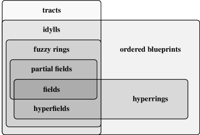
Figure 1. Comparison of different algebraic structures

Note that we consider idylls as both tracts and ordered blueprints, which makes sense since there is an adjunction between the categories of tracts and ordered blueprints that retricts to an equivalence precisely for idylls. In this sense, an idyll can be thought of an object that is both a tract and an ordered blueprint; cf. Theorem 2.21 for more details.

We now turn to giving a more precise definition of ordered blueprints and matroids over them.

1.2.4. Ordered blueprints

An ordered semiring is a semiring $R$ together with a partial order $\leqslant$ that is compatible with multiplication and addition. (See section 2.6 for a more precise definition.)

An ordered blueprint is a triple $B=(B^{\bullet},B^{+},\leqslant)$ where $(B^{+},\leqslant)$ is an ordered semiring and $B^{\bullet}$ is a multiplicative subset of $B^{+}$ which generates $B^{+}$ as a semiring and contains $0$ and $1$.

A morphism of ordered blueprints $(B^{\bullet}_{1},B^{+}_{1},\leqslant_{1})$ and $(B^{\bullet}_{2},B^{+}_{2},\leqslant_{2})$ is an order-preserving morphism $f:B^{+}_{1}\to B^{+}_{2}$ of semirings with $f(B^{\bullet}_{1})\subset B^{\bullet}_{2}$.

We denote the category of ordered blueprints by $\operatorname{{OBlpr}}$.

Example 1.1.

A hyperfield is an algebraic structure similar to a field, but where addition is allowed to be multivalued (see Section 2.3 for a precise definition). We can identify a hyperfield $F$ with an ordered blueprint $F^{\textup{oblpr}}$ as follows:

• The associated semiring $(F^{\textup{oblpr}})^{+}$ is the free semiring ${\mathbb{N}}[F^{\times}]$ over the multiplicative group $F^{\times}$.

• The underlying monoid $(F^{\textup{oblpr}})^{\bullet}$ is $(F,\cdot)$.

• The partial order $\leqslant$ of $(F^{\textup{oblpr}})^{+}$ is generated by the relations $0\leqslant\sum a_{i}$ whenever $0\in\boxplus a_{i}$.

Example 1.2.

A partial field $P$ is a certain equivalence class of pairs $(G,R)$ consisting of a commutative ring $R$ with $1$ and a subgroup $G\leqslant R^{\times}$ containing $-1$. (See section 2.2 for a more precise definition.) We can identify a partial field $P$ with an ordered blueprint $P^{\textup{oblpr}}$ as follows:

• The associated semiring $(P^{\textup{oblpr}})^{+}$ is ${\mathbb{N}}[G]$.

• The underlying monoid $(P^{\textup{oblpr}})^{\bullet}$ is $G\cup\{0\}$.

• The partial order $\leqslant$ is generated by the 3-term relations $0\leqslant a+b+c$ whenever $a,b,c\in G$ satisfy $a+b+c=0$ in $R$.

An example of particular interest is the ordered blueprint associated with the regular partial field ${\mathbb{U}}_{0}=(\{-1,0,1\},{\mathbb{Z}})$, whose associated ordered blueprint ${{\mathbb{F}}_{1}^{\pm}}$ corresponds to the submonoid $\{0,1,-1\}$ of ${\mathbb{Z}}$ together with the partial order generated by $0\leqslant 1+(-1)$.

The ordered blueprints associated to hyperfields and partial fields are in fact ordered blue fields, meaning that $B=B^{\times}\bigcup\{0\}$, where $B^{\times}$ denotes the set of invertible elements of $B$. They are also ${{\mathbb{F}}_{1}^{\pm}}$-algebras, a notion which will be defined shortly.

The category of ordered blueprints has an initial object called ${{\mathbb{F}}_{1}}$ with associated semiring ${\mathbb{N}}$, underlying monoid $\{0,1\}$ (with the usual multiplication), and partial order given by equality.

1.2.5. Some properties of ordered blueprints

The category of ordered blueprints admits pushouts: given morphisms $B\to C$ and $B\to D$ of ordered blueprints, one can form their tensor product $C\otimes_{B}D$, which satisfies the universal property of a fiber coproduct.

One can also form the localization $S^{-1}B$ of an ordered blueprint $B$ with respect to any multiplicative subset $S$, and it has the usual universal property.

1.2.6. ${{\mathbb{F}}_{1}^{\pm}}$-algebras

An ${{\mathbb{F}}_{1}^{\pm}}$-algebra is an ordered blueprint $B$ together with a morphism ${{\mathbb{F}}_{1}^{\pm}}\to B$. Equivalently, an ${{\mathbb{F}}_{1}^{\pm}}$-algebra is an ordered blueprint $B$ together with an element $\myepsilon$ of $B$ that satisfies $0\leqslant 1+\myepsilon$. This element $\myepsilon$ plays the role of $-1$ in this theory, and is crucial for defining structures such as matroids. We denote the full subcategory of ${{\mathbb{F}}_{1}^{\pm}}$-algebras by $\operatorname{{OBlpr}}_{{\mathbb{F}}_{1}^{\pm}}$.

1.2.7. Idylls as ${{\mathbb{F}}_{1}^{\pm}}$-algebras

The ordered blueprints associated to hyperfields and partial fields are ${{\mathbb{F}}_{1}^{\pm}}$-algebras. More generally, if $F=(G,N_{G})$ is any idyll in the sense of section 1.2.2, we can consider $F$ as an ${{\mathbb{F}}_{1}^{\pm}}$-algebra $F^{\textup{oblpr}}$ as follows:

• The associated semiring $(F^{\textup{oblpr}})^{+}$ is ${\mathbb{N}}[G]$.

• The underlying monoid $(F^{\textup{oblpr}})^{\bullet}$ is $G\cup\{0\}$.

• The partial order $\leqslant$ is generated by the relations $0\leqslant\sum a_{i}$ whenever $a_{i}\in G$ satisfy $\sum a_{i}\in N_{G}$ in ${\mathbb{N}}[G]$.

One can characterize ordered blueprints of the form $F^{\textup{oblpr}}$ for some idyll $F$ among all ordered blueprints in a simple way: they are precisely the ${{\mathbb{F}}_{1}^{\pm}}$-algebras that of the form $(B^{\times}\cup\{0\},{\mathbb{N}}[B^{\times}],\leqslant)$ for which $0\leqslant 1+a$ only if $a=\myepsilon$ and that are purely positive, meaning that $\leqslant$ is generated by elements of the form $0\leqslant\sum a_{i}$.

1.2.8. Matroids over ${{\mathbb{F}}_{1}^{\pm}}$-algebras

Let $B$ be an ${{\mathbb{F}}_{1}^{\pm}}$-algebra, let $E$ be a finite totally ordered set, and let $r\in{\mathbb{N}}$. We denote by $\binom{E}{r}$ the family of all $r$-element subsets of $E$.

A Grassmann-Plücker function of rank $r$ on $E$ with coefficients in $B$ is a function $\myvarphi:\binom{E}{r}\to B$ such that:

• $\myvarphi(I)\in B^{\times}$ for some $I\in\binom{E}{r}$.

• $\myvarphi$ satisfies the Plücker relations

  $$0\leqslant\sum_{k=0}^{r}\myepsilon^{k}\myvarphi(I\backslash i_{k})\myvarphi(J\cup i_{k})$$

  whenever $J\in\binom{E}{r-1}$ and $I=\{i_{0},\ldots,i_{r}\}\in\binom{E}{r+1}$ with $i_{0}<\cdots<i_{r}$. (We set $\myvarphi(J\cup i)=0$ if $i\in J$.)

We say that two Grassmann-Plücker functions $\myvarphi,\myvarphi^{\prime}:\binom{E}{r}\to B$ are equivalent if $\myvarphi=a\myvarphi^{\prime}$ for some $a\in B^{\times}$.

A $B$-matroid of rank $r$ on $E$ is an equivalence class of Grassmann-Plücker functions. We denote by $\operatorname{\mathpzc{Mat}}_{B}(r,E)$ the set of all $B$-matroids of rank $r$ on $E$.

If $F$ is an idyll, an $F$-matroid of rank $r$ on $E$ in the above sense is the same thing as a strong $F$-matroid of rank $r$ on $E$ in the sense of [4]. In this case, we can characterize (strong) $F$-matroids of rank $r$ on $E$ in several different cryptomorphic ways, e.g. in terms of circuits, dual pairs, or vectors (see [2, 4] or sections 3.1.4 and 3.1.6 below).

The definition of $\operatorname{\mathpzc{Mat}}_{B}(r,E)$ is functorial: if $f:B\to C$ is a morphism of ${{\mathbb{F}}_{1}^{\pm}}$-algebras, there is an induced map $f_{*}:\operatorname{\mathpzc{Mat}}_{B}(r,E)\to\operatorname{\mathpzc{Mat}}_{C}(r,E)$.

If $F$ is an idyll and $f:F\to{\mathbb{K}}$ is the canonical morphism to the final object ${\mathbb{K}}$ (which is shorthand for ${\mathbb{K}}^{\textup{oblpr}}$) of the category of idylls, the push-forward $\underline{M}:=f_{*}(M)$ is a ${\mathbb{K}}$-matroid, i.e. a matroid in the usual sense. We call $\underline{M}$ the underlying matroid of $M$.

If $M^{\prime}$ is a matroid, we say that $M^{\prime}$ is weakly (resp. strongly) representable over an idyll $F$ if $M^{\prime}=f_{*}(M)$ for some weak (resp. strong) $F$-matroid $M$. This generalizes the usual notion of representability over fields, or more generally partial fields (for which the notions of weak and strong $F$-matroids coincide).

1.3. Part 2: Constructing moduli spaces of matroids

As discussed above, we wish to construct a moduli space $\operatorname{Mat}(r,E)$ of rank-$r$ matroids on $E$ as a ordered blue scheme (over ${{\mathbb{F}}_{1}^{\pm}}$) which represents a certain functor. In order to formulate precisely what this means, and in particular to specify which moduli functor we wish to represent, we first provide the reader with a gentle introduction to the theory of ordered blue schemes.

1.3.1. Ordered blue schemes

One constructs the category of ordered blue schemes, starting from ordered blueprints, much in the same way that one constructs the category of schemes starting from commutative rings. We give just a brief synopsis here; see section 4.1 for further details.

Let $B$ be an ordered blueprint.

A monoid ideal of $B$ is a subset $I$ of $B$ such that $0\in I$ and $IB=I$ where $IB=\{ab\mid a\in I,b\in B\}$.

A prime ideal of $B$ is a monoid ideal whose complement is a multiplicative subset.

The spectrum $\operatorname{Spec}B$ of $B$ is constructed as follows:

• The topological space of $X=\operatorname{Spec}B$ consists of the prime ideals of $B$, and comes with the topology generated by the principal opens

  $$U_{h}\ =\ \{\,{\mathfrak{p}}\in\operatorname{Spec}B\,|\,h\notin{\mathfrak{p}}\,\}$$

  for $h\in B$.

• The structure sheaf ${\mathcal{O}}_{X}$ is the unique sheaf on $X$ with the property that ${\mathcal{O}}_{X}(U_{h})=B[h^{-1}]$ for all $h\in B$. The stalk of ${\mathcal{O}}_{X}$ at a point $x\in X$ corresponding to ${\mathfrak{p}}$ is $B_{\mathfrak{p}}$.

An ordered blueprinted space is a topological space $X$ together with a sheaf ${\mathcal{O}}_{X}$ in $\operatorname{{OBlpr}}$. Such spaces form a category $\operatorname{{OBlprSp}}$. A morphism $f:B\to C$ of ordered blueprints defines a morphism $f^{\ast}:\operatorname{Spec}C\to\operatorname{Spec}B$ of $\operatorname{{OBlpr}}$-spaces. This defines the contravariant functor $\operatorname{Spec}:\ \operatorname{{OBlpr}}\ \longrightarrow\ \operatorname{{OBlprSp}}$ whose essential image is the category of affine ordered blue schemes.

An ordered blue scheme is an $\operatorname{{OBlpr}}$-space that has an open covering by affine ordered blue schemes $U_{i}$. A morphism of ordered blue schemes is a morphism of $\operatorname{{OBlpr}}$-spaces. We denote the category of ordered blue schemes by $\operatorname{OBSch}$.

An ordered blue ${{\mathbb{F}}_{1}^{\pm}}$-scheme is an ordered blue scheme $X$ for which ${\mathcal{O}}_{X}(U)$ has the structure of an ${{\mathbb{F}}_{1}^{\pm}}$-algebra for every open subset $U$ of $X$. We denote the full subcategory of ordered blue ${{\mathbb{F}}_{1}^{\pm}}$-schemes by $\operatorname{OBSch}_{{\mathbb{F}}_{1}^{\pm}}$.

1.3.2. Some properties of ordered blue schemes

Ordered blue schemes possess many familiar properties from the world of schemes. For example:

• The global section functor $\Gamma:\operatorname{OBSch}\to\operatorname{{OBlpr}}$ defined by $\Gamma(X,{\mathcal{O}}_{X}):={\mathcal{O}}_{X}(X)$ is a left inverse to $\operatorname{Spec}$. In particular, $B\cong\Gamma(\operatorname{Spec}B)$.

• The category $\operatorname{OBSch}$ contains fibre products, and in the affine case $\operatorname{Spec}(B)\times_{\operatorname{Spec}(D)}\operatorname{Spec}(C)\cong\operatorname{Spec}(B\otimes_{D}C)$.

Various familiar objects from algebraic geometry have analogues in the context of ordered blue schemes; for example, one can define an invertible sheaf on an ordered blue scheme $X$ to be a sheaf which is locally isomorphic to the structure sheaf ${\mathcal{O}}_{X}$ of $X$. There is a tensor product operation which turns the set $\operatorname{Pic}X$ of isomorphism classes of invertible sheaves on $X$ into an abelian group.

Similarly, one can define, for each $n\in{\mathbb{N}}$ and each ordered blueprint $B$, the projective $n$-space ${\mathbb{P}}^{n}_{B}$ as an ordered blue scheme over $\operatorname{Spec}(B)$.

1.3.3. Families of matroids

Let $X$ be an ordered blue ${{\mathbb{F}}_{1}^{\pm}}$-scheme. A Grassmann–Plücker function of rank $r$ on $E$ over $X$ is an invertible sheaf ${\mathcal{L}}$ on $X$ together with a map $\myvarphi:\binom{E}{r}\to\Gamma(X,{\mathcal{L}})$ such that $\{\myvarphi(I)\}_{I\in\binom{E}{r}}$ generate ${\mathcal{L}}$ and the $\myvarphi(I)$ satisfy the Plücker relations in $\Gamma(X,{\mathcal{L}}^{\otimes 2})$ (see Definition 5.1 for a more precise definition).

Two such functions $({\mathcal{L}},\myvarphi)$ and $({\mathcal{L}}^{\prime},\myvarphi^{\prime})$ are said to be isomorphic if there is an isomorphism from ${\mathcal{L}}$ to ${\mathcal{L}}^{\prime}$ taking $\myvarphi$ to $\myvarphi^{\prime}$.

A matroid bundle of rank $r$ on the set $E$ over $X$ is an isomorphism class of Grassmann–Plücker functions.

If $X=\operatorname{Spec}(B)$ is an affine ordered blue ${{\mathbb{F}}_{1}^{\pm}}$-scheme, it turns out that a matroid bundle over $X$ is the same thing as a $B$-matroid.

1.3.4. The moduli functor of matroids

One can extend the (covariant) functor taking an ${{\mathbb{F}}_{1}^{\pm}}$-algebra $B$ to $\operatorname{\mathpzc{Mat}}(r,E)(B)$ to a (contravariant) functor $\operatorname{\mathpzc{Mat}}(r,E):\operatorname{OBSch}_{{\mathbb{F}}_{1}^{\pm}}\to\operatorname{Sets}$ taking $X$ to the set of matroid bundles of rank $r$ on $E$ over $X$.

We prove the following theorem, cf. Theorem 5.5:

Theorem A.

The moduli functor $\operatorname{\mathpzc{Mat}}(r,E)$ is representable by an ordered blue ${{\mathbb{F}}_{1}^{\pm}}$-scheme $\operatorname{Mat}(r,E)$. In particular, for every ordered blue ${{\mathbb{F}}_{1}^{\pm}}$-scheme $X$ there is a natural bijection

$$\operatorname{Hom}_{{{\mathbb{F}}_{1}^{\pm}}}(X,\operatorname{Mat}(r,E)){\buildrel\sim\over{\longrightarrow}}\operatorname{\mathpzc{Mat}}(r,E)(X).$$

The moduli space $\operatorname{Mat}(r,E)$ is constructed as an ordered blue subscheme of ${\mathbb{P}}^{N}_{{\mathbb{F}}_{1}^{\pm}}$, where $N=\#\binom{E}{r}-1$. (This is analogous to the Plücker embedding of the Grassmannian $\operatorname{Gr}(r,n)$.) However, making this precise requires developing some foundational material on line bundles, the “Proj” construction, etc. in the context of ordered blue schemes.

1.4. Part 3: Applications to matroid theory

We conclude this introduction by providing a more detailed overview of Part 3 of the paper, in which we connect various algebraic structures related to the moduli spaces $\operatorname{Mat}(r,E)$ to concepts such as realization spaces, cross ratios, rescaling classes, and universal partial fields which have been previously studied in the matroid theory literature.

1.4.1. Universal idylls

Given a (classical) matroid $M$, we can associate to $M$ a universal idyll $k_{M}$, which is derived from a certain “residue ordered blue field” of the matroid space $\operatorname{Mat}(r,E)$.

More precisely, a classical matroid $M$ corresponds to a morphism $\mychi_{M}:\operatorname{Spec}{\mathbb{K}}\to\operatorname{Mat}(r,E)$ which we call the characteristic morphism of $M$. Topologically, $\operatorname{Spec}{\mathbb{K}}$ is a point, and the image point $x_{M}$ in the ordered blue ${{\mathbb{F}}_{1}^{\pm}}$-scheme $\operatorname{Mat}(r,E)$ of the characteristic morphism has an associated residue idyll, much as every point of a (classical) scheme has an associated residue field. We call the residue idyll $k_{M}$ of $x_{M}$ the universal idyll of $M$.

1.4.2. Realization spaces

Let $K$ be a field. The realization space over $K$ of a rank-$r$ matroid $M$ on $E=\{1,\ldots,n\}$ is the subset of the Grassmannian $\operatorname{Gr}(r,n)$ consisting of sub-vector spaces of $K^{n}$ whose associated matroid is $M$. Such realization spaces have been used for proving that several moduli spaces, such as Hilbert schemes and moduli spaces of curves, can have arbitrarily complicated singularities, cf. [57].

Given a matroid $M$ and an idyll $F$, the realization space ${\mathcal{X}}_{M}(F)$ is the set of isomorphism classes of $F$-matroids whose underlying matroid is $M$. More precisely, let $\Delta:\binom{E}{r}\to{\mathbb{K}}$ be a Grassmann-Plücker function, $M$ the corresponding matroid, and $\mychi_{M}:\operatorname{Spec}({\mathbb{K}})\to\operatorname{Mat}(r,E)$ its characteristic morphism. The canonical map from $F$ to ${\mathbb{K}}$ (which takes $0$ to $0$ and every nonzero element of $F$ to $1$) induces a natural map $\Phi:\ \operatorname{Mat}(r,E)(F)\ \longrightarrow\ \operatorname{Mat}(r,E)({\mathbb{K}})$ taking an $F$-matroid to its underlying matroid. With this notation, the realization space ${\mathcal{X}}_{M}(F)$ of $M$ over $F$ is the fibre of $\Phi$ over $\mychi_{M}$.

Realization spaces are functorial with respect to morphisms of idylls.

The functor from idylls to sets taking an idyll $F$ to the realization space ${\mathcal{X}}_{M}(F)$ is represented by the universal idyll $k_{M}$. In other words, there is a canonical bijection

$${\rm Hom}(k_{M},F){\buildrel\sim\over{\longrightarrow}}{\mathcal{X}}_{M}(F)$$

which is functorial in $F$.

1.4.3. The weak matroid space

So far we have been talking more or less exclusively about strong matroids in the sense of [4]. However, there is also a notion of weak matroids over an idyll $F$ which is quite important in many contexts.

A weak Grassmann-Plücker function of rank $r$ on $E$ with coefficients in an idyll $F$ is a function

$$\textstyle\Delta:\ \binom{E}{r}\ \longrightarrow\ F$$

whose support is the set of bases of a matroid and which satisfies the $3$-term Plücker relations

$$0\ \leqslant\ \Delta(I_{1,2})\,\Delta(I_{3,4})\ +\ \myepsilon\,\Delta(I_{1,3})\,\Delta(I_{2,4})\ +\ \Delta(I_{1,4})\,\Delta(I_{2,3})$$

for every $(r-2)$-subset $I$ of $E$ and all $i_{1}<i_{2}<i_{3}<i_{4}$ with $i_{1},i_{2},i_{3},i_{4}\notin I$, where $I_{k,l}=I\cup\{i_{k},i_{l}\}$.

Two weak Grassmann-Plücker functions $\Delta$ and $\Delta^{\prime}$ are equivalent if $\Delta=a\Delta^{\prime}$ for some element $a\in F^{\times}$.

A weak $F$-matroid of rank $r$ on $E$ is an equivalence class $M$ of weak Grassmann-Plücker functions $\Delta$ of rank $r$ on $E$ with coefficients in $F$. We denote the set of all weak $F$-matroids of rank $r$ on $E$ by $\operatorname{\mathpzc{Mat}}^{w}(r,E)(F)$.

The weak matroid space $\operatorname{Mat}^{w}(r,E)$ is defined analogously to $\operatorname{Mat}(r,E)$, with the important difference that we only impose $3$-term Plücker relations; see section 6.4 for a precise definition. For a matroid $M$, we define the universal pasture $k_{M}^{w}$ as the residue idyll of the space of weak matroids at the point corresponding to $M$. We can also define the weak realization space ${\mathcal{X}}_{M}^{w}(F)$ of $M$ over $F$ to be the set of all weak $F$-matroids whose underlying matroid is $M$.

As in the strong case, there is a canonical bijection

$${\rm Hom}(k_{M}^{w},F){\buildrel\sim\over{\longrightarrow}}{\mathcal{X}}^{w}_{M}(F)$$

which is functorial in $F$.

1.4.4. Cross ratios

Four points on a projective line over a field $K$ correspond to a point of the Grassmannian $\operatorname{Gr}(2,4)$ over $K$, and their cross ratio can be expressed in terms of the Plücker coordinates of this point. This reinterpretation allows for a generalization of cross ratios to higher Grassmannians and also to non-realizable matroids.

Let $F$ be an idyll and $M$ be a matroid of rank $r$ on $E$. The cross ratios of $M$ in $F$ are indexed by the set $\Omega_{M}$ of $4$-tuples ${\mathcal{I}}=(I,i_{1},i_{2},i_{3},i_{4})\in\binom{E}{r-2}\times E^{4}$ for which $I_{1,2}$, $I_{2,3}$, $I_{3,4}$ and $I_{4,1}$ are bases of $M$, where $I_{k,l}=I\cup\{i_{k},i_{l}\}$.

Let $F$ be an idyll and let $M$ be a weak $F$-matroid defined by the weak Grassmann-Plücker function $\Delta:\binom{E}{r}\to F$. The cross ratio function of $M$ is the function $\operatorname{Cr}_{M}:\Omega_{M}\to F^{\times}$ that sends an element ${\mathcal{I}}=(I,i_{1},i_{2},i_{3},i_{4})$ of $\Omega_{M}$ to

$$\operatorname{Cr}_{M}({\mathcal{I}})\ =\ \frac{\Delta(I_{1,2})\cdot\Delta(I_{3,4})}{\Delta(I_{2,3})\cdot\Delta(I_{4,1})}.$$

One checks easily that this depends only on the equivalence class of $\Delta$, and is thus a well-defined function of $M$.

1.4.5. Foundations

Let $B$ be an ${{\mathbb{F}}_{1}^{\pm}}$-algebra. A fundamental element of $B$ is an element $a\in B$ such that $0\leqslant a+b+\myepsilon$ for some $b\in B$.

The foundation of $B$ is the subblueprint $B^{\textup{found}}$ of $B$ generated by the fundamental elements of $B$. Taking foundations is a functorial construction.

The relevance of this notion for matroid theory is that cross ratios of weak $F$-matroids are fundamental elements of $F$ (which is a simple consequence of the 3-term Plücker relations).

If $M$ is a matroid, we define the foundation of $M$, denoted $k_{M}^{f}$, to be the foundation of the universal pasture $k_{M}^{w}$ of $M$. Since the functor taking an idyll $F$ to the weak realization space ${\mathcal{X}}^{w}_{M}(F)$ is represented by $k_{M}^{w}$, and cross ratios of weak $F$-matroids are fundamental elements of $F$, there is a natural universal cross ratio function $\operatorname{Cr}_{M}^{\textup{univ}}:\Omega_{M}\to k_{M}^{f}$.

We prove that the foundation $k_{M}^{f}$ of $M$ is generated by the universal cross ratios $\operatorname{Cr}_{M}^{\textup{univ}}(\Omega_{M})$ over ${{\mathbb{F}}_{1}^{\pm}}$.

We also show (cf. Theorem 7.17) that for every matroid $M$ and idyll $F$, the following are equivalent: (a) $M$ is weakly representable over $F$; (b) $M$ is weakly representable over $F^{\textup{found}}$; and (c) there exists a morphism $k_{M}^{f}\to F$.

1.4.6. The Tutte group and inner Tutte group

The Tutte group ${\mathbb{T}}_{M}$ of a matroid $M$ was introduced by Dress and Wenzel in [16] as a tool for studying the representability of matroids by algebraically encoding results such as Tutte’s homotopy theorem (cf. [54] and [55]).

The Tutte group is usually defined in terms of generators and relations, and several “cryptomorphic” presentations of this group are known. Our approach allows for an intrinsic definition of the Tutte group ${\mathbb{T}}_{M}$ as the unit group of the universal pasture $k_{M}^{w}$ (see section 6.5 for details).

Dress and Wenzel also define a certain subgroup ${\mathbb{T}}_{M}^{(0)}$ of the Tutte group ${\mathbb{T}}_{M}$ which they call the inner Tutte group. Using their results, we show that the natural isomorphism $(k_{M}^{w})^{\times}\to{\mathbb{T}}_{M}$ restricts to an isomorphism $(k_{M}^{f})^{\times}\to{\mathbb{T}}_{M}^{(0)}$. In other words, the inner Tutte group of $M$ is the unit group of the foundation of $M$.

1.4.7. Rescaling classes

Let $M$ be a matroid of rank $r$ on $E$. The importance of the foundation of $M$ is that it represents the functor which takes an idyll $F$ to the set of rescaling classes of $F$-matroids with underlying matroid $M$, in the same way the universal idyll (resp. universal pasture) of $M$ represents the realization space ${\mathcal{X}}_{M}(F)$ (resp. weak realization space ${\mathcal{X}}_{M}^{w}(F)$).

Let $F$ be an idyll, and let $T(F)$ be the group of functions $t:E\to F^{\times}$. The rescaling class of an $F$-matroid $M$ is the $T(F)$-orbit of $M$ in $\operatorname{Mat}^{w}(r,E)(F)$, where $T(F)$ acts on a weak Grassmann-Plücker function $\Delta:\binom{E}{r}\to F$ by the formula

$$t.\Delta(I)\ =\ \prod_{i\in I}t(i)\cdot\Delta(I).$$

Rescaling classes are the natural generalization to matroids over arbitrary idylls of reorientation classes for oriented matroids, where two (realizable) oriented matroids are considered reorientation equivalent if they correspond to the isomorphic real hyperplane arrangements. (For non-realizable matroids, there is a similar assertion involving pseudosphere arrangements; this is part of the famous "Topological Representation Theorem" of Folkman and Lawrence, cf. [20] or [7, section 5.2].)

If we fix a matroid $M$ and an idyll $F$, we define the rescaling class space ${\mathcal{X}}^{f}_{M}(F)$ to be the set of rescaling classes of weak $F$-matroids with underlying matroid $M$. There is a canonical bijection

$$\operatorname{Hom}(k_{M}^{f},F){\buildrel\sim\over{\longrightarrow}}{\mathcal{X}}_{M}^{f}(F)$$

which is functorial in $F$.

As a sample motivation for considering rescaling classes over more general idylls than just the hyperfield of signs, we mention that while it is true that a matroid $M$ is regular (i.e., representable over the rational numbers by a totally unimodular matrix) if and only if $M$ is representable over ${{\mathbb{F}}_{1}^{\pm}}$, there are in general many non-isomorphic ${{\mathbb{F}}_{1}^{\pm}}$-matroids whose underlying matroid is a given regular matroid $M$. However, there is always precisely one rescaling class over ${{\mathbb{F}}_{1}^{\pm}}$. In other words, regular matroids are the same thing as rescaling classes of ${{\mathbb{F}}_{1}^{\pm}}$-matroids.

1.4.8. Foundations of binary and regular matroids

A binary matroid is a matroid that is representable over the finite field ${\mathbb{F}}_{2}$ with two elements.

We show that a matroid is regular if and only if its foundation is ${{\mathbb{F}}_{1}^{\pm}}$, and binary if and only if its foundation is either ${{\mathbb{F}}_{1}^{\pm}}$ or ${\mathbb{F}}_{2}$. We recover from these observations a new proof of the well-known facts that (a) a matroid is regular if and only if it is representable over every field; and (b) a binary matroid is either representable over every field or not representable over any field of characteristic different from $2$.

We also use these observations to give new and conceptual proofs of the following facts: (a) a binary matroid has at most one rescaling class over every idyll (compare with [60, Thm. 6.9]); and (b) every matroid has at most one rescaling class over ${\mathbb{F}}_{3}$ (cf. [8]).

In addition, we show (cf. Theorem 7.35) that a matroid $M$ is regular if and only if $M$ is binary and weakly representable over some idyll $F$ with $1\neq\myepsilon$ . This implies, for example (taking $F$ to be the hyperfield of signs) the well-known fact that a matroid is regular if and only if it is both binary and orientable.

1.4.9. Relation to the universal partial field of Pendavingh and van Zwam

The universal partial field ${\mathbb{P}}_{M}$ of a matroid $M$ was introduced by Pendavingh and van Zwam in [48]. It has the property that a matroid $M$ is representable over a partial field $P$ if and only if there is a partial field homomorphism ${\mathbb{P}}_{M}\to P$.

We show that there is a partial field $P_{M,0}$ naturally derived from the universal pasture $k_{M}^{w}$ of $M$ with the property that for every partial field $P$ there is a natural bijection

$$\operatorname{Hom}(P_{M,0},P){\buildrel\sim\over{\longrightarrow}}{\mathcal{X}}_{M}(P^{\textup{oblpr}})$$

which is functorial in $P$.

The universal partial field of Pendavingh and van Zwam is isomorphic to the partial subfield ${\mathbb{P}}_{M}$ of $P_{M,0}$ generated by the cross ratios of $M$. We prove that for every partial field $P$ there is a natural and functorial bijection

$$\operatorname{Hom}({\mathbb{P}}_{M},P){\buildrel\sim\over{\longrightarrow}}{\mathcal{X}}_{M}^{f}(P^{\textup{oblpr}}).$$

One disadvantage of the universal partial field is that it doesn’t always exist: there are matroids (e.g. the Vámos matroid) which are not representable over any partial field. However, every matroid is representable over some idyll, so the foundation $k_{M}^{f}$ of $M$ gives us information about representations of $M$ even when the universal partial field is undefined.

Our classification of binary and regular matroids in terms of their foundations also yields a classification of such matroids in terms of their universal partial fields: a matroid is regular if and only if its universal partial field is ${{\mathbb{F}}_{1}^{\pm}}$, and binary if and only if its universal partial field is ${{\mathbb{F}}_{1}^{\pm}}$ or ${\mathbb{F}}_{2}$.

Part I Idylls, ordered blueprints, and matroids

2. The interplay between partial fields, hyperfields, fuzzy rings, tracts, and ordered blueprints

Our approach to matroid bundles utilizes an interplay between tracts and ordered blueprints, as introduced by the first author and Bowler in [4] and the second author in [36], respectively. Tracts and ordered blueprints are common generalizations of other algebraic structures that appear in matroid theory, such as partial fields, hyperfields, and fuzzy rings.

In this section, we review the definitions of all of the aforementioned notions and explain their interdependencies. Our exposition culminates in Theorem 2.21, which exhibits a diagram of comparison functors between the corresponding categories.

2.1. Semirings

Since many of the following concepts are based on semirings and derived notions, we begin with an exposition of semirings. All of our structures will be commutative and, following the practice of the literature in commutative algebra and algebraic geometry, we omit the adjective “commutative” when speaking of semirings, monoids, and other structures.

A monoid is a commutative semigroup with a neutral element. A monoid morphism is a multiplicative map that preserves the neutral element. In this text, a semiring is a set $R$ together with two binary operations $+$ and $\cdot$ and with two constants $0$ and $1$ such that the following axioms are satisfied:

1. $(R,+,0)$ is a monoid;

2. $(R,\cdot,1)$ is a monoid;

3. $0\cdot a=0$ for all $a\in R$;

4. $a(b+c)=ab+ac$ for all $a,b,c\in R$.

A morphism of semirings is a map $f:R_{1}\to R_{2}$ between semirings $R_{1}$ and $R_{2}$ such that

$$f(0)\ =\ 0,\qquad f(1)\ =\ 1,\qquad f(a+b)\ =\ f(a)+f(b)\qquad\text{and}\qquad f(ab)\ =\ f(a)f(b)$$

for all $a,b\in R_{1}$. We denote the category of semirings by $\operatorname{{SRings}}$.

Let $R$ be a semiring. An ideal of $R$ is a subset $I$ such that $0\in I$, $a+b\in I$ and $ac\in I$ for all $a,b\in I$ and $c\in R$. An ideal is proper if it is not equal to $R$.

Given any subset $S=\{a_{i}\}_{i\in I}$ of elements of $R$, we define the ideal $\langle S\rangle=\langle a_{i}\rangle_{i\in I}$ generated by $S$ as the smallest ideal of $R$ containing $S$, which is equal to

$$\langle S\rangle\quad=\quad\bigcap_{\begin{subarray}{c}\text{ideals }J\\ \text{with }S\subset J\end{subarray}}J\quad=\quad\big{\{}\,\sum_{i\in I}b_{i}a_{i}\in R\,\big{|}\,b_{i}\in R\text{ with }b_{i}=0\text{ for almost all }i\in I\,\big{\}}.$$

The group of units of $R$ is the group $R^{\times}$ of all multiplicatively invertible elements of $R$. A semifield is a semiring $R$ such that $R=R^{\times}\cup\{0\}$.

Note that an ideal $I$ is proper if and only if $I\cap R^{\times}=\emptyset$. A semiring $R$ is a semifield if and only if $\{0\}$ and $R$ are the only ideals of $R$.

Example 2.1.

Every (commutative and unital) ring is a semiring. Examples of semirings that are not rings are the natural numbers ${\mathbb{N}}$ and the nonnegative real numbers ${\mathbb{R}}_{\geqslant 0}$. Examples of a more exotic nature are the tropical numbers ${\mathbb{R}}_{\geqslant 0}$ together with the usual multiplication and the tropical addition $a+b=\max\{a,b\}$, and the Boolean numbers ${\mathbb{B}}=\{0,1\}$ with $1+1=1$, which appears simultaneous as a subsemiring and as a quotient of the tropical numbers.

2.1.1. Monoid semirings

Let $A$ be a multiplicatively written monoid and $R$ a semiring. The monoid semiring $R[A]$ consists of all finite formal $R$-linear combinations $\sum r_{a}a$ of elements $a$ of $A$, i.e. almost all $r_{a}\in R$ are zero. The addition and multiplication of $R[A]$ are defined by the formulas

$$\Big{(}\sum_{a\in A}r_{a}a\Big{)}+\Big{(}\sum_{a\in A}s_{a}a\Big{)}\ =\ \sum_{a\in A}(r_{a}+s_{a})a\quad\text{and}\quad\Big{(}\sum_{a\in A}r_{a}a\Big{)}\cdot\Big{(}\sum_{a\in A}s_{a}a\Big{)}\ =\ \sum_{a\in A}\Big{(}\sum_{bc=a}r_{b}s_{c}\Big{)}a,$$

respectively. The zero of $R[A]$ is $0=\sum 0\cdot a$ and its multiplicative identity is $1=\sum r_{a}a$ with $r_{1}=1$ and $r_{a}=0$ for $a\neq 1$.

This construction comes with an inclusion $A\to R[A]$, and we often identify $A$ with its image in $R[A]$, i.e. we write $b$ or $1\cdot b$ for the element $\sum r_{a}a$ of $R[A]$ with $r_{b}=1$ and $r_{a}=0$ for $a\neq b$. In the case $R={\mathbb{N}}$, every element of ${\mathbb{N}}[A]$ is a sum $\sum a_{i}$ of elements $a_{i}$ in $A$.

Example 2.2.

Polynomial semirings are particular examples of monoid semirings. Let $R$ be a semiring and let $A=\{\prod_{i=1}^{n}T_{i}^{e_{i}}\;|\;e_{i}\in{\mathbb{N}}\}$ be the monoid of all monomials in $T_{1},\dotsc,T_{n}$. Then $R[A]$ is the polynomial semiring $R[T_{1},\dotsc,T_{n}]$.

2.2. Partial fields

In [52], Semple and Whittle introduced partial fields as a tool for studying representability questions about matroids. The theory of matroid representations over partial fields was developed further by Pendavingh and van Zwam in [48] and [49]; also cf. van Zwam’s thesis [58]. Loosely speaking, a partial field can be thought of as a set $P$ together with distinguished elements $0$ and $1$, a map $\cdot:P\times P\to P$, and a partially defined map $+:P\times P\to P$ satisfying:

• $(P,\cdot,1)$ is a commutative monoid in which every nonzero element is invertible

• $+$ is associative and commutative with neutral element $0$

• every element $a\in P$ has a unique additive inverse $-a$

• multiplication distributes over addition.

Morphisms of partial fields are defined to be structure preserving maps.

It is somewhat involved to make the requirements on $+$ rigorous; in particular, the formulation of the associativity of $+$ involves binary rooted trees with labelled leaves.

Van Zwam gives in [58, section 2.1] a simpler but equivalent description of partial fields in terms of a ring $R$ together with a subgroup $G$ of the unit group $R^{\times}$ of $R$ that contains $-1$. The downside of this approach is that morphisms are not structure preserving maps; in particular, the isomorphism type of the ambient ring $R$ is not determined by a partial field. There is, however, a distinguished ambient ring for every partial field, which has better properties than other choices for $R$, cf. [58, Thm. 2.6.11]. This latter observation leads us to the following hybrid of Semple-Whittle’s and van Zwam’s definitions.

Let ${\mathbb{Z}}[G]$ be the group ring of a group $G$, which comes together with the inclusion $G\cup\{0\}\to{\mathbb{Z}}[G]$, sending $a\in G$ to $1\cdot a$ and $0$ to $0$.

A partial field $P=(P^{\times},\mypi_{P})$ is a commutative group $P^{\times}$ together with a surjective ring homomorphism $\mypi_{P}:{\mathbb{Z}}[P^{\times}]\to R_{P}$ such that

1. the composition $P^{\times}\cup\{0\}\longrightarrow{\mathbb{Z}}[P^{\times}]\stackrel{{\scriptstyle\mypi_{P}}}{{\longrightarrow}}R_{P}$ is injective;

2. for every $a\in P^{\times}$, there is a unique element $b\in P^{\times}$ such that $\mypi_{P}(a+b)=0$;

3. the kernel of $\mypi_{P}$ is generated by all elements $a+b+c$ with $a,b,c\in P^{\times}\cup\{0\}$ such that $\mypi_{P}(a+b+c)=0$.

We can recover the motivating properties of a partial field from these axioms:

• we define $P^{\times}\cup\{0\}$ as the underlying set of $P$, i.e. $P$ is a subset of the ambient ring $R_{P}$;

• we write $a+b=c$ for elements $a,b,c\in P$ with $\mypi_{P}(a+b+(-c))=0$, which defines the partial addition $+$ of $P$;

• if $\mypi_{P}(a+b)=0$, then $\mypi_{P}(b)=\mypi_{P}((-1)\cdot a)$, i.e. every element $a\in P$ has a unique additive inverse with respect to the partial addition of $P$, which we denote by $-a$.

A morphism $f:P_{1}\to P_{2}$ of partial fields is a group homomorphism $P^{\times}_{1}\to P^{\times}_{2}$ that extends to a ring homomorphism $R_{P_{1}}\to R_{P_{2}}$. Using the notation introduced above, this is the same as a map $f:P_{1}\to P_{2}$ such that $f(0)=0$, $f(1)=1$, $f(ab)=f(a)f(b)$ for all $a,b\in P_{1}$ and $f(a)+f(b)=f(c)$ if $a+b=c$ with $a,b,c\in P_{1}$. We denote the category of partial fields by $\operatorname{{PartFields}}$.

Example 2.3.

A field $K$ can be identified with the partial field $(K^{\times},\mypi_{K})$, where $\mypi_{K}:{\mathbb{Z}}[K^{\times}]\to K$ is the surjective ring homomorphism induced by the identity map $K^{\times}\cup\{0\}\to K$. Note that with this identification a field homomorphism is the same as a morphism between the associated partial fields.

The regular partial field ${\mathbb{U}}_{0}$ consists of the group ${\mathbb{U}}_{0}^{\times}=\{\pm 1\}$ and the surjective ring homomorphism $\mypi_{{\mathbb{U}}_{0}}:{\mathbb{Z}}[{\mathbb{U}}_{0}^{\times}]\to{\mathbb{Z}}$ mapping $\pm 1$ to the corresponding elements in ${\mathbb{Z}}$. Note that it is an initial object in the category of partial fields. Later on, this partial field will be reincarnated as the ordered blue field ${{\mathbb{F}}_{1}^{\pm}}$, cf. Example 2.19.

For an extensive list of other examples, we refer to [58].

2.3. Hyperfields and hyperrings

The notion of an algebraic structure in which addition is allowed to be multi-valued goes back to Frédéric Marty, who introduced hypergroups in 1934 ([42]). Later on, in the mid-1950’s, Marc Krasner ([30]) developed the theory of hyperrings and hyperfields in the context of approximating non-Archimedean fields, and in the 1990’s Murray Marshall ([41]) explored connections to the theory of real spectra and spaces of orderings. Subsequent advocates of hyperstructures included Oleg Viro ([59], in connection with tropical geometry) and Connes and Consani ([10], in connection with geometry over ${{\mathbb{F}}_{1}}$).

A commutative hypergroup is a set $G$ together with a distinctive element $0$ and a hyperaddition, which is a map

$$\,\raisebox{-1.1pt}{\larger[-0]{$\boxplus$}}\,:\quad G\times G\quad\longrightarrow\quad{\mathcal{P}}(G)$$

into the power set ${\mathcal{P}}(G)$ of $G$, such that:

1. $a\,\raisebox{-1.1pt}{\larger[-0]{$\boxplus$}}\,b$ is not empty, (nonempty sums)

2. $\bigcup_{d\in b\,\raisebox{-1.1pt}{\larger[-0]{$\boxplus$}}\,c}a\,\raisebox{-1.1pt}{\larger[-0]{$\boxplus$}}\,d=\bigcup_{d\in a\,\raisebox{-1.1pt}{\larger[-0]{$\boxplus$}}\,b}d\,\raisebox{-1.1pt}{\larger[-0]{$\boxplus$}}\,c$, (associativity)

3. $0\,\raisebox{-1.1pt}{\larger[-0]{$\boxplus$}}\,a=a\,\raisebox{-1.1pt}{\larger[-0]{$\boxplus$}}\,0=\{a\}$, (neutral element)

4. there is a unique element $-a$ in $G$ such that $0\in a\,\raisebox{-1.1pt}{\larger[-0]{$\boxplus$}}\,(-a)$, (inverses)

5. $a\,\raisebox{-1.1pt}{\larger[-0]{$\boxplus$}}\,b=b\,\raisebox{-1.1pt}{\larger[-0]{$\boxplus$}}\,a$, (commutativity)

6. $c\in a\,\raisebox{-1.1pt}{\larger[-0]{$\boxplus$}}\,b$ if and only if $(-a)\in(-c)\,\raisebox{-1.1pt}{\larger[-0]{$\boxplus$}}\,b$ (reversibility)

for all $a,b,c\in G$. Note that thanks to commutativity and associativity, it makes sense to define hypersums of several elements $a_{1},\dotsc,a_{n}$ unambiguously by the recursive formula

$$\operatorname*{\,\raisebox{-2.2pt}{\larger[2]{$\boxplus$}}\,}_{i=1}^{n}\ a_{i}\ =\ \bigcup_{b\in\operatorname*{\,\raisebox{-2.2pt}{\larger[2]{$\boxplus$}}\,}_{i=1}^{n-1}a_{i}}b\,\raisebox{-1.1pt}{\larger[-0]{$\boxplus$}}\,a_{n}.$$

A (commutative) hyperring is a set $R$ together with distinctive elements $0$ and $1$ and with maps $\,\raisebox{-1.1pt}{\larger[-0]{$\boxplus$}}\,:R\times R\to{\mathcal{P}}(R)$ and $\cdot:R\times R\to R$ such that

1. $(R,\,\raisebox{-1.1pt}{\larger[-0]{$\boxplus$}}\,,0)$ is a commutative hypergroup,

2. $(R,\cdot,1)$ is a commutative monoid,

3. $0\cdot a=a\cdot 0=0$,

4. $a\cdot(b\,\raisebox{-1.1pt}{\larger[-0]{$\boxplus$}}\,c)=ab\,\raisebox{-1.1pt}{\larger[-0]{$\boxplus$}}\,ac$

for all $a,b,c\in R$ where $a\cdot(b\,\raisebox{-1.1pt}{\larger[-0]{$\boxplus$}}\,c)=\{ad|d\in b\,\raisebox{-1.1pt}{\larger[-0]{$\boxplus$}}\,c\}$. Note that the reversibility axiom (HG6) for the hyperaddition follows from the other axioms of a hyperring.

A morphism of hyperrings is a map $f:R_{1}\to R_{2}$ between hyperrings such that

$$f(0)\ =\ 0,\qquad f(1)\ =\ 1,\qquad f(a\,\raisebox{-1.1pt}{\larger[-0]{$\boxplus$}}\,b)\ \subset\ f(a)\,\raisebox{-1.1pt}{\larger[-0]{$\boxplus$}}\,f(b)\qquad\text{and}\qquad f(ab)\ =\ f(a)\cdot f(b)$$

for all $a,b\in R_{1}$ where $f(a\,\raisebox{-1.1pt}{\larger[-0]{$\boxplus$}}\,b)=\{f(c)|c\in a\,\raisebox{-1.1pt}{\larger[-0]{$\boxplus$}}\,b\}$. We denote the category of hyperrings by $\operatorname{{HypRings}}$.

The unit group $R^{\times}$ of a hyperring $R$ is the group of all multiplicatively invertible elements in $R$. A hyperfield is a hyperring $K$ such that $0\neq 1$ and $K=K^{\times}\cup\{0\}$. We denote the full subcategory of hyperfields in $\operatorname{{HypRings}}$ by $\operatorname{{HypFields}}$.

Example 2.4.

Every ring $R$ can be considered as a hyperring by defining $a\,\raisebox{-1.1pt}{\larger[-0]{$\boxplus$}}\,b=\{a+b\}$. If $R$ is a field, the corresponding hyperring is a hyperfield.

The Krasner hyperfield is the hyperfield ${\mathbb{K}}=\{0,1\}$ whose addition is characterized by $1\,\raisebox{-1.1pt}{\larger[-0]{$\boxplus$}}\,1=\{0,1\}$. Note that all other sums and products are determined by the hyperring axioms. It is a terminal object in $\operatorname{{HypFields}}$.

The tropical hyperfield ${\mathbb{T}}$ was introduced by Viro in [59]. Its multiplicative monoid consists of the non-negative real numbers ${\mathbb{R}}_{\geqslant 0}$, together with the usual multiplication, and its hyperaddition is defined by the rule $a\,\raisebox{-1.1pt}{\larger[-0]{$\boxplus$}}\,b=\max\{a,b\}$ if $a\neq b$ and $a\,\raisebox{-1.1pt}{\larger[-0]{$\boxplus$}}\,a=[0,a]$. The tropical hyperfield has a particular importance for valuations and tropical geometry, since a nonarchimedean absolute value $v:K\to{\mathbb{R}}_{\geqslant 0}$ on a field $K$ is the same thing as a morphism $v:K\to{\mathbb{T}}$ of hyperfields.

The sign hyperfield ${\mathbb{S}}$ is the multiplicative monoid ${\mathbb{S}}=\{0,\pm 1\}$ together with the hyperaddition characterized by $1\,\raisebox{-1.1pt}{\larger[-0]{$\boxplus$}}\,1=\{1\}$, $(-1)\,\raisebox{-1.1pt}{\larger[-0]{$\boxplus$}}\,(-1)=\{-1\}$, and $1\,\raisebox{-1.1pt}{\larger[-0]{$\boxplus$}}\,(-1)=\{-1,0,1\}$. Note that with this definition, the sign map ${\mathbb{R}}\to{\mathbb{S}}$ becomes a morphism of hyperfields.

There is a more general construction of hyperfields, as quotients of fields by a multiplicative subgroup, which covers all of the previous examples. Let $K$ be a field and $G$ a multiplicative subgroup of $K^{\times}$. Then the quotient $K/G$ of $K$ by the action of $G$ on $K$ by multiplication carries a natural structure of a hyperfield: we have $(K/G)^{\times}=K^{\times}/G$ as an abelian group and

$$[a]\,\raisebox{-1.1pt}{\larger[-0]{$\boxplus$}}\,[b]\ =\ \big{\{}\ [c]\ \big{|}\ c=a^{\prime}+b^{\prime}\text{ for some }a^{\prime}\in[a],b^{\prime}\in[b]\ \big{\}}$$

for classes $[a]$ and $[b]$ of $K/G$.

Example 2.5.

The Krasner hyperfield and the tropical hyperfield are instances of a construction that applies to all totally ordered idempotent semirings. Namely, every idempotent semiring $R$ comes with a natural partial order $\leqslant$ defined by declaring that $a\leqslant b$ if $a+b=b$. If $R$ is bipotent, i.e. $a+b\in\{a,b\}$ for all $a,b\in R$, then $R$ is totally ordered with respect to $\leqslant$.

When $R$ is totally ordered, we can define a hyperaddition on $R$ as

$$a\,\raisebox{-1.1pt}{\larger[-0]{$\boxplus$}}\,b\ =\ \begin{cases}\{a+b\}&\text{if }a\neq b,\\ \{c\in R\,|\,c\leqslant a\}&\text{if }a=b.\end{cases}$$

The set $R$, together with its usual multiplication and the hyperaddition  [-0]$\boxplus$ , is a hyperring. (The only nontrivial thing to check is associativity of the hyperaddition, which requires the total order of $R$). If $R$ is a totally ordered idempotent semifield, this procedure turns $R$ into a hyperfield.

2.4. Fuzzy rings

We review the definition of a fuzzy ring from [15] in a slightly simplified but evidently equivalent form. As a second step, we give a yet simpler description of the category of fuzzy rings by exhibiting a representative of a particularly simple form in each isomorphism class. We refer the reader to section 2.1 for all preliminary definitions on semirings.

A fuzzy ring is a possibly nondistributive semiring $R$, i.e. it might disobey axiom (SR4) of a semiring, together with a proper ideal $I$ that satisfies the following axioms for all $a,b,c,d\in R$:

1. there is a unique $\myepsilon\in R^{\times}$ such that $1+\myepsilon\in I$;

2. $a+b,c+d\in I$ implies $ac+\myepsilon bd\in I$.

3. $a\in R^{\times}$ implies $a(b+c)=ab+ac$;

4. $a+b(c+d)\in I$ implies $a+bc+bd\in I$;

Here $R^{\times}=\{\,a\in R\,|\,ab=1\text{ for some }b\in R\,\}$ denotes the unit group of $R$.

Since these axioms might look bewildering to the reader that sees them for the first time, we include a brief discussion to motivate them. The idea behind this definition is that the zero of a field becomes replaced by the ideal $I$; consequently additive inverses only exist “up to $I$”.

Axiom (FR1) implies that every unit $a\in R^{\times}$ has a unique additive inverse in $R^{\times}$, which is $\myepsilon a$. In particular, we have $\myepsilon^{2}=1$. Axioms (FR3) and (FR4) are weakened forms of distributivity—these axioms hold automatically in a distributive semiring. Axiom (FR2) is reminiscent of the arithmetic of quotient rings: $a\equiv\myepsilon b\pmod{I}$ and $c\equiv\myepsilon d\pmod{I}$ implies $ac\equiv bd\pmod{I}$ and thus $ab+\myepsilon bd\in I$.

Example 2.6.

A standard example is the fuzzy ring associated with a field $K$, which is given by $R=\{S\subset K\;|\;S\neq\emptyset\}$ with addition $S+T=\{s+t\;|\;s\in S,t\in T\}$ and multiplication $S\cdot T=\{st\;|\;s\in S,t\in T\}$ and whose ideal is $I=\{S\subset K\;|\;0\in S\}$. Another example is the group semiring ${\mathbb{N}}[G]$ of an abelian group $G$ together with a proper ideal $I$ of ${\mathbb{N}}[G]$ such that (FR1) and (FR2) hold—axioms (FR3) and (FR4) are automatically satisfied since ${\mathbb{N}}[G]$ is distributive.

A morphism $R_{1}\to R_{2}$ of fuzzy rings is a group homomorphism $f:R_{1}^{\times}\to R_{2}^{\times}$ such that $\sum a_{i}\in I_{1}$ implies $\sum f(a_{i})\in I_{2}$ for all $a_{1},\dotsc,a_{n}\in R_{1}^{\times}$. We denote the category of fuzzy rings by $\operatorname{{FuzzRings}}$.

Note that Dress also defines homomorphisms of fuzzy rings in [15]. Since this latter notion does not have a particular meaning for matroid theory, we omit it from our exposition. Note further that morphisms and homomorphisms were renamed in [24] as weak and strong morphisms, respectively.

It follows immediately from the definition that a morphism of fuzzy rings preserves $1$ and $\myepsilon$. It is also apparent that it depends only on the respective subsets of $R_{1}$ and $R_{2}$ whose elements can be written as a sum of units. This observation leads to the following fact.

Proposition 2.7.

Let $(R,I)$ be a fuzzy ring with unit group $G=R^{\times}$ and $\mypi:{\mathbb{N}}[G]\to R$ the natural map that sends a finite formal sum $\sum a_{i}$ of elements $a_{i}\in G$ to its sum in $R$. Define $J=\mypi^{-1}(I)$. Then $\overline{R}=({\mathbb{N}}[G],J)$ is a fuzzy ring and the identity map $G\to R^{\times}$ defines an isomorphism of fuzzy rings $\overline{R}\to R$.

Proof.

We include a brief proof. For more details, we refer the reader to Appendix B of [4].

Since $I\subset R$ is a proper ideal, $R^{\times}\cap I=\emptyset$ and thus $J\cap G=\emptyset$, i.e. $J$ is proper. It follows from the definition that $J$ is an ideal of ${\mathbb{N}}[G]$. Properties (FR3) and (FR4) of a fuzzy ring are satisfied since ${\mathbb{N}}[G]$ is distributive. Properties (FR1) and (FR2) follow immediately from the definition of $J$ as $\mypi^{-1}(I)$ and the validity of (FR1) and (FR2) in $R$.

It is also clear from the definition of $\overline{R}$ that the identity maps $\textup{id}:G\to R^{\times}$ and $\textup{id}:R^{\times}\to G$ are mutually inverse isomorphisms of fuzzy rings. ∎

Corollary 2.8.

The category $\operatorname{{FuzzRings}}$ is equivalent to its full subcategory consisting of fuzzy rings of the form $({\mathbb{N}}[G],I)$ for some abelian group $G$. Given an abelian group $G$ and a proper ideal $I\subset{\mathbb{N}}[G]$, the pair $({\mathbb{N}}[G],I)$ is a fuzzy ring if and only if it satisfies (FR1) and (FR2). A morphism between two fuzzy rings of the form $({\mathbb{N}}[G_{1}],I_{1})$ and $({\mathbb{N}}[G_{2}],I_{2})$ is the same as a semiring homomorphism $f:{\mathbb{N}}[G_{1}]\to{\mathbb{N}}[G_{2}]$ with $f(G_{1})\subset G_{2}$ and $f(I_{1})\subset I_{2}$.

Proof.

The first claim follows immediately from Proposition 2.7. The second claim follows since ${\mathbb{N}}[G]$ is distributive and thus satisfies (FR3) and (FR4) automatically. To conclude, a group homomorphism $f:G_{1}\to G_{2}$ extends uniquely to a semiring homomorphism $\tilde{f}:{\mathbb{N}}[G_{1}]\to{\mathbb{N}}[G_{2}]$. The homomorphism $f$ is a morphism of fuzzy rings if and only if $\sum a_{i}\in I_{1}$ implies $\sum f(a_{i})\in I_{2}$, i.e. if $\tilde{f}(I_{1})\subset I_{2}$. Thus the last claim. ∎

Example 2.9.

As we will see in Theorem 2.21, partial fields and hyperfields can be realized as fuzzy rings in a natural way. They represent somewhat opposite ends of a spectrum: while the sum of any two elements of a hyperfield needs to contain at least $1$ element, the sum of two elements of a partial field is equal to at most $1$ element.

The fuzzy ring associated with the regular partial field ${\mathbb{U}}_{0}$ is initial in $\operatorname{{FuzzRings}}$ and it is not associated with any hyperfield. The fuzzy ring associated with the Krasner hyperfield ${\mathbb{K}}$ is terminal in $\operatorname{{FuzzRings}}$ and it is not associated with any partial field.

We describe some examples of fuzzy rings that are neither partial fields nor hyperfields. Let $n$ be an even integer and $\mymu_{n}$ a cyclic group with $n$ elements, generated by an element $\myzeta_{n}$. Let $I$ be the ideal of ${\mathbb{N}}[\mymu_{n}]$ that is generated by the elements

$$\sum_{i=1}^{n/d}\ \myzeta_{n}^{id}$$

where $d$ ranges through the divisors of $n$ smaller than $n$. Then $F=({\mathbb{N}}[\mymu_{n}],I)$ is a fuzzy ring, which does not come from a hyperfield since $\myzeta_{n}+\myzeta_{n}$ is not defined. If $n$ is divisible by a prime larger than $3$, then $F$ does not come from a partial field since $I$ is not generated by only $3$-term sums.

Another class of examples is the following. Let $G$ be a group with neutral element $1$ and $I$ the ideal of ${\mathbb{N}}[G]$ that is generated by $1+1$ and $1+1+1$. Then $F=({\mathbb{N}}[G],I)$ is a fuzzy ring, which does not come from a partial field since it would require that $0=1+1+1=1+0=1$. If $G$ contains an element $a\neq 1$, then $F$ does not come from a hyperfield since $1\,\raisebox{-1.1pt}{\larger[-0]{$\boxplus$}}\,a$ would have to be empty.

Both of the above examples can be realized as partial hyperfields, as considered in [4], which are (roughly speaking) hyperfields that are allowed to disobey the nonemptiness axiom (HG1). Though partial hyperfields and fuzzy rings are closely related, there are technical differences between them stemming from the different roles of the associative law in the two settings. This is discussed in detail in [24]; in particular, cf. Example 4.2.

2.5. Tracts

In the recent joint work [4], the first author and Nathan Bowler distill from the aforementioned theories of partial fields, hyperfields, and fuzzy rings the notion of a tract, which seems to be both a natural setting for matroid theory and a relatively simple (yet quite general) algebraic structure.

A tract $F=(F^{\times},N_{F})$ is an abelian group $F^{\times}$ together with a subset $N_{F}$ of the group semiring ${\mathbb{N}}[F^{\times}]$, called the nullset of $F$, satisfying the following properties:

1. $0\in N_{F}$ and $1\notin N_{F}$;

2. $aN_{F}=N_{F}$ for every $a\in F^{\times}$;

3. there is a unique element $\myepsilon\in F^{\times}$ such that $1+\myepsilon\in N_{F}$.

We sometimes write $F$ for the set $F^{\times}\cup\{0\}$, and we think of $N_{F}$ as the linear combinations of elements of $F$ which “sum to zero”.

Let $F_{i}=(F_{i}^{\times},N_{F_{i}})$ be tracts for $i=1,2$. A morphism $f:F_{1}\to F_{2}$ of tracts is a group homomorphism $F_{1}^{\times}\to F_{2}^{\times}$ such that the induced homomorphism ${\mathbb{N}}[F_{1}^{\times}]\to{\mathbb{N}}[F_{2}^{\times}]$ maps $N_{F_{1}}$ to $N_{F_{2}}$. Equivalently, it is a map $f:F_{1}\to F_{2}$ such that $f(0)=0$, $f(1)=1$, $f(ab)=f(a)f(b)$ for all $a,b\in F_{1}$ and $\sum f(a_{i})\in N_{F_{2}}$ for all $\sum a_{i}\in N_{F_{1}}$. We denote the category of tracts by $\operatorname{{Tracts}}$.

We recall some facts about tracts from [4].

Lemma 2.10.

Let $F$ be a tract and $\myepsilon\in F^{\times}$ the unique element with $1+\myepsilon\in N_{F}$. Then we have

1. $F\cap N_{F}=\{0\}$;

2. $\myepsilon^{2}=1$;

3. $a+\myepsilon a\in N_{F}$ for every $a\in F^{\times}$;

4. if $a+b\in N_{F}$ with $a,b\in F^{\times}$, then $b=\myepsilon a$.

Example 2.11.

The tract $(\{1\},{\mathbb{N}}-\{1\})$ associated to the Krasner hyperfield ${\mathbb{K}}$ is terminal in $\operatorname{{Tracts}}$. More generally, every fuzzy ring $({\mathbb{N}}[G],I)$ defines a tract $(G,I)$ as we will see in Theorem 2.21. In fact, there are only two ways in which a tract can fail to come from a fuzzy ring.

The first deviation of tracts from fuzzy rings lies in the fact that the nullset $N_{F}$ of a tract does not have to be an ideal of the semiring ${\mathbb{N}}[F^{\times}]$, but merely an $F^{\times}$-invariant subset. For example, the nullset $N_{F}=\{0,1+\myepsilon\}$ of the initial object $F=(\{1,\myepsilon\},N_{F})$ of $\operatorname{{Tracts}}$ is not an ideal of ${\mathbb{N}}[\{1,\myepsilon\}]$.

Another example is the following. If $F=(G,I)$ is a tract, for instance coming from a fuzzy ring $({\mathbb{N}}[G],I)$, then we can consider the $3$-term truncation

$$I_{3}\ =\ \big{\{}\,a+b+c\,\big{|}\,a+b+c\in I\text{ and }a,b,c\in G\cup\{0\}\,\big{\}}$$

of $I$, which is not an ideal of ${\mathbb{N}}[G]$, but merely a $G$-invariant set. The resulting tract $(G,I_{3})$ can be a useful gadget to compare strong $F$-matroids, which are defined by all Plücker relations, with weak $F$-matroids, which are defined in terms of just the $3$-term Plücker relations.

The second deviation of tracts from fuzzy rings stems from the omission of axiom (FR2) of a fuzzy ring. The following is an example of a tract whose nullset is an ideal, but which does not come from a fuzzy ring due to the failure of axiom (FR2).

Let $F=({\mathbb{F}}_{5}^{\times},N_{F})$ be the subtract of ${\mathbb{F}}_{5}=\{0,1,2,3,4\}$ that consists of the same underlying monoid, but whose nullset is the ideal $N_{F}$ of ${\mathbb{N}}[F^{\times}]$ generated by the elements $1+4$ and $1+1+3$. Then $F=(F^{\times},N_{F})$ is a tract with $\myepsilon=4$. If $({\mathbb{N}}[F^{\times}],N_{F})$ was a fuzzy ring, then (FR2) applied to $a=c=1+1$ and $b=d=3$ would imply that

$$(1+1)(1+1)+4\cdot 3\cdot 3\ =\ 1+1+1+1+1$$

is an element of $N_{F}$, which is not the case. (Note that $4\cdot 3\cdot 3=36\equiv 1$ modulo $5$.)

2.6. Ordered blueprints

As a general reference for ordered blueprints, we refer the reader to Chapter 5 of the second author’s lecture notes [38].

An ordered semiring is a semiring $R$ together with a partial order $\leqslant$ that is compatible with multiplication and addition, i.e. $x\leqslant y$ and $z\leqslant t$ imply $x+z\leqslant y+t$ and $xz\leqslant yt$ for all $x,y,z,t\in R$.

An ordered blueprint is a triple $B=(B^{\bullet},B^{+},\leqslant)$ where $(B^{+},\leqslant)$ is an ordered semiring and $B^{\bullet}$ is a multiplicative subset of $B^{+}$ that generates $B^{+}$ as a semiring and contains $0$ and $1$. A morphism of ordered blueprints $(B^{\bullet}_{1},B^{+}_{1},\leqslant_{1})$ and $(B^{\bullet}_{2},B^{+}_{2},\leqslant_{2})$ is an order preserving morphism $f:B^{+}_{1}\to B^{+}_{2}$ of semirings with $f(B^{\bullet}_{1})\subset B^{\bullet}_{2}$. We denote the category of ordered blueprints by $\operatorname{{OBlpr}}$.

Let $B=(B^{\bullet},B^{+},\leqslant)$ be an ordered blueprint. We call $B^{\bullet}$ the underlying monoid of $B$ and think of it as the underlying set, i.e. we write $a\in B$ for $a\in B^{\bullet}$. Note that a morphism $f:B_{1}\to B_{2}$ of ordered blueprints is determined by its restriction $f^{\bullet}:B^{\bullet}_{1}\to B^{\bullet}_{2}$ to the underlying monoids. We call $B^{+}$ be associated semiring of $B$. We call $\leqslant$ the partial order of $B$.

Typically, we denote the elements of $B^{\bullet}$ by $a$, $b$, $c$ and $d$, and the elements of $B^{+}$ by either $x$, $y$, $z$ and $t$ or by $\sum a_{i}$, $\sum b_{j}$, $\sum c_{k}$ and $\sum d_{l}$ where assume that the $a_{i}$, $b_{j}$, $c_{k}$ and $d_{l}$ are in $B^{\bullet}$. Note that every element of $B^{+}$ is indeed a sum of elements in $B^{\bullet}$.

The unit group $B^{\times}$ of an ordered blueprint is the commutative group of all multiplicatively invertible elements of $B$. An ordered blue field is an ordered blueprint $B$ with $B^{\bullet}=B^{\times}\cup\{0\}$.

If we have $\sum a_{i}\leqslant\sum b_{j}$ and $\sum b_{j}\leqslant\sum a_{i}$, then we write $\sum a_{i}\equiv\sum b_{j}$. If this is the case for all relations in $B$, then we say that $B$ is an algebraic blueprint. (Algebraic blueprints are simply called “blueprints” in [37].)

Remark 2.12.

Note that the partial order of $B$ corresponds to what is called the subaddition of $B$ in [36] in the following way: the subaddition of $B$ is the preorder on the monoid semiring ${\mathbb{N}}[B^{\bullet}]$ that is the pullback of $\leqslant$ along the quotient map ${\mathbb{N}}[B^{\bullet}]\to B^{+}$.

The following constructions provide a rich class of examples of ordered blueprints.

2.6.1. Semirings and monoids

Every semiring $R$ defines the ordered blueprint $(R,R,=)$ where $=$ denotes the trivial partial order given by equality of elements. A monoid with zero, which is a (multiplicatively written) commutative semigroup $A$ with neutral element $1$ and absorbing element $0$ (i.e. $0\cdot a=0$ for all $a\in A$), defines the ordered blueprint $(A,{\mathbb{N}}[A],=)$. In what follows, we identify semirings and monoids with their associated ordered blueprints and say that an ordered blueprint $B$ is a semiring or a monoid if it is isomorphic to an ordered blueprint coming from a semiring or monoid with zero, respectively.

Example 2.13.

The monoid ${{\mathbb{F}}_{1}}=\{0,1\}$, sometimes referred to as the field with one element, can be identified with the ordered blueprint $(\{0,1\},{\mathbb{N}},=)$, and the Boolean semifield ${\mathbb{B}}=\{0,1\}$ (where $1+1=1$) can be identified with $(\{0,1\},{\mathbb{B}},=)$.

2.6.2. Free algebras

Given an ordered blueprint $B$ and a set $X=\{T_{i}\}_{i\in I}$, we can form the free ordered blueprint $B[X]=B[T_{i}]_{i\in I}$ over $B$, which is defined as follows. The associated semiring $B[X]^{+}$ is the usual polynomial semiring over $B^{+}$ in the variables $T_{i}$. The underlying monoid $B[X]^{\bullet}$ is the subset of monomials $a\prod T_{i}^{n_{i}}$ with coefficients $a\in B$. The partial order $\leqslant$ of $B[X]^{+}$ is the smallest partial order that contains the partial order of $B^{+}$ and that is closed under multiplication and addition.

Example 2.14.

The free algebra ${\mathbb{C}}[T]=({\mathbb{C}}[T]^{\bullet},{\mathbb{C}}[T]^{+},=)$ is the ordered blueprint where ${\mathbb{C}}[T]^{+}$ is the usual polynomial ring and ${\mathbb{C}}[T]^{\bullet}$ is the subset of all terms of the form $aT^{n}$ with $a\in{\mathbb{C}}$ and $n\in{\mathbb{N}}$. The free algebra ${{\mathbb{F}}_{1}}[T]$ is the ordered blueprint where ${{\mathbb{F}}_{1}}[T]^{+}={\mathbb{N}}[T]^{+}$ is the usual polynomial semiring over ${\mathbb{N}}$, endowed with the trivial order $=$, and where ${{\mathbb{F}}_{1}}[T]^{\bullet}$ consists of all monomials and $0$.

Remark 2.15.

The reader might be alarmed by the fact that the notation $B[T]$ for the free ordered blueprint conflicts with the notation for corresponding notation for semirings: given a semiring $R$, the blueprint $(R[T],R[T],=)$ associated with the polynomial semiring $R[T]$ differs from the free blueprint $R[T]=(R[T]^{\bullet},R[T]^{+},\leqslant_{R[T]})$. More precisely, if $B=R$ and $B[T]$ is the free ordered blueprint, then the polynomial semiring $R[T]$ equals $B[T]^{+}$. However, it will be clear from the context to which construction we refer when we write $B[T]$ or $R[T]$. Sometimes we indicate that we mean the latter construction by writing $B[T]^{+}$.

2.6.3. Quotients by relations

Given an ordered blueprint $B=(B^{\bullet},B^{+},\leqslant_{B})$ and a set of relations $S=\{x_{i}\leqslant y_{i}\}_{i\in I}$, which we do not assume to be contained in $\leqslant_{B}$, we define the ordered blueprint $C=B\!\sslash\!\langle S\rangle$ as the following triple $(C^{\bullet},C^{+},\leqslant_{C})$. Let $\leqslant^{\prime}$ be the smallest preorder on $B^{+}$ that contains $\leqslant_{B}$ and $S$ and that is closed under multiplication and addition. We write $x\equiv y$ if $x\leqslant y$ and $y\leqslant x$. Then $\equiv$ is an equivalence relation on $B^{+}$, and we define $C^{+}$ as $B^{+}/\equiv$, which inherits naturally the structure of an ordered blueprint since $\leqslant^{\prime}$ is closed under multiplication and addition. The preorder $\leqslant^{\prime}$ induces a partial order $\leqslant_{C}$ on $C^{+}$, which turns $C^{+}$ into an ordered semiring. The multiplicative subset $C^{\bullet}$ is defined as the image of $B^{\bullet}$ under the quotient map $B^{+}\to C^{+}$.

Given an ordered blueprint $B=(B^{\bullet},B^{+},\leqslant)$, we say that the partial order $\leqslant$ of $B$ is generated by a set $S=\{x_{i}\leqslant y_{i}\}_{i\in I}$ of relations on $B^{+}$ if $\leqslant$ is the smallest preorder on $B^{+}$ that contains $S$ and that is closed under multiplication and addition.

Example 2.16.

With this construction, we can define ordered blueprints like ${{\mathbb{F}}_{1^{2}}}=\{0,1,-1\}\!\sslash\!\langle 0\equiv 1+(-1)\rangle$ (note that in this case ${\mathbb{F}}_{1^{2}}^{+}={\mathbb{Z}}$) and ${\mathbb{B}}[T_{1},\dotsc,T_{6}]\!\sslash\!\langle 0\leqslant T_{1}T_{6}+T_{2}T_{5}+T_{3}T_{4}\rangle$.

2.6.4. Subblueprints

Let $B=(B^{\bullet},B^{+},\leqslant_{B})$ be an ordered blueprint. An (ordered) subblueprint of $B$ is an ordered blueprint $C$ such that $C^{\bullet}$ is a submonoid of $B^{\bullet}$, such that the ambient semiring $C^{+}$ is the subsemiring of $B^{+}$ that is generated by $C^{\bullet}$ and such that the partial order of $C$ is the restriction of the partial order of $B^{+}$ to $C^{+}$. Note that by definition, every submonoid $C^{\bullet}$ of $B^{\bullet}$ determines a unique subblueprint $C$ of $B$.

2.6.5. Tensor products

Given two morphisms $B\to C$ and $B\to D$ of ordered blueprints, there exists a push-out of the diagram $C\leftarrow B\to D$, which is represented by the tensor product $C\otimes_{B}D$ of $C$ and $D$ over $B$. The tensor product is constructed as follows.

The semiring $(C\otimes_{B}D)^{+}$ is the usual tensor product $C^{+}\otimes_{B^{+}}D^{+}$ of commutative semirings, whose elements are classes of finite sums $\sum c_{i}\otimes d_{i}$ of pure tensors $c_{i}\otimes d_{i}$ with respect to the usual identifications. The monoid $(C\otimes_{B}D)^{\bullet}$ is defined as the subset of all pure tensors of $(C\otimes_{B}D)^{+}$. The partial order on $(C\otimes_{B}D)^{+}$ is defined as the smallest partial order that is closed under addition and multiplication and that contains all relations of the forms

$$\textstyle\sum a_{i}\otimes 1\leqslant\sum c_{k}\otimes 1\qquad\text{and}\qquad\sum 1\otimes b_{j}\leqslant\sum 1\otimes d_{l}$$

for which $\sum a_{i}\leqslant\sum c_{k}$ in $C$ and $\sum b_{j}\leqslant\sum d_{l}$ in $D$, respectively.

Example 2.17.

The tensor product can be used to extend constants. For instance, we have ${{\mathbb{F}}_{1}}[T_{1},\dotsc,T_{n}]\otimes_{{\mathbb{F}}_{1}}B=B[T_{1},\dotsc,T_{n}]$ for every ordered blueprint $B$. Given a semiring $R$, the tensor product $R\otimes_{{\mathbb{F}}_{1}}{{\mathbb{F}}_{1^{2}}}=R\otimes_{\mathbb{N}}{\mathbb{Z}}$ is the ring of differences associated with $R$.

2.7. ${{\mathbb{F}}_{1}^{\pm}}$-algebras and idylls

As we will see in Theorem 2.21, the ordered blueprint that corresponds to the regular partial field ${\mathbb{U}}_{0}$ under the embedding of $\operatorname{{PartFields}}$ in $\operatorname{{OBlpr}}$ is ${{\mathbb{F}}_{1}^{\pm}}=\{0,1,\myepsilon\}\!\sslash\!\langle 0\leqslant 1+\myepsilon\rangle$.

An ${{\mathbb{F}}_{1}^{\pm}}$-algebra is an ordered blueprint $B$ together with a morphism $\myalpha_{B}:{{\mathbb{F}}_{1}^{\pm}}\to B$, which we call the structure map of $B$. We denote the image $\myalpha_{B}(\myepsilon)$ of $\myepsilon\in{{\mathbb{F}}_{1}^{\pm}}$ by $\myepsilon_{B}$, or simply by $\myepsilon$ if there is no danger of confusion. This element plays the role of $-1$, and for a given for $a\in B$, we call $\myepsilon a$ the weak inverse of $a$. Note that we do not use the symbol $-1$ in this context since $1$ does not have an additive inverse in the ambient semiring $B^{+}$, i.e. $B^{+}$ is in general not a ring. (${{\mathbb{F}}_{1}^{\pm}}$ itself provides an example: $({{\mathbb{F}}_{1}^{\pm}})^{+}={\mathbb{N}}[1,\myepsilon]$.)

A morphism of ${{\mathbb{F}}_{1}^{\pm}}$-algebras from an ${{\mathbb{F}}_{1}^{\pm}}$-algebra $B$ to an ${{\mathbb{F}}_{1}^{\pm}}$-algebra $C$ is a morphism $f:B\to C$ of ordered blueprints that commutes with the respective structure maps $\myalpha_{B}$ and $\myalpha_{C}$. Equivalently, it is a morphism of ordered blueprints $f:B\to C$ such that $f(\myepsilon_{B})=\myepsilon_{C}$. This defines the category $\operatorname{{OBlpr}}_{{\mathbb{F}}_{1}^{\pm}}$ of ${{\mathbb{F}}_{1}^{\pm}}$-algebras.

The weak inverse $\myepsilon a$ of an element $a$ of an ${{\mathbb{F}}_{1}^{\pm}}$-algebra is in general not uniquely determined by the relation $0\leqslant a+\myepsilon a$. For instance, we have $0\leqslant 1\otimes 1+\myepsilon\otimes 1$ and $0\leqslant 1\otimes 1+1\otimes\myepsilon$ in ${{\mathbb{F}}_{1}^{\pm}}\otimes_{{\mathbb{F}}_{1}}{{\mathbb{F}}_{1}^{\pm}}$. For certain purposes, we want to impose the condition that $b=\myepsilon a$ is uniquely determined by the realtion $0\leqslant a+b$. We call an ${{\mathbb{F}}_{1}^{\pm}}$-algebra ${{\mathbb{F}}_{1}^{\pm}}\to B$ with this property an ${{\mathbb{F}}_{1}^{\pm}}$-algebra with unique weak inverses. This defines a full subcategory $\operatorname{{OBlpr}}^{\pm}$ of $\operatorname{{OBlpr}}_{{\mathbb{F}}_{1}^{\pm}}$. The following definition captures the class of ordered blueprints that come from tracts.

Definition 2.18.

An ordered blueprint $B$ is purely positive if its partial order is generated by relations of the form $0\leqslant\sum a_{i}$. An idyll is a purely positive ${{\mathbb{F}}_{1}^{\pm}}$-algebra $B$ with unique weak inverses that is an ordered blue field and for which the natural map ${\mathbb{N}}[B^{\times}]\to B^{+}$ is a bijection.

Since the element $\myepsilon$ of an ${{\mathbb{F}}_{1}^{\pm}}$-algebra $B$ with unique weak inverses is uniquely determined by $0\leqslant 1+\myepsilon$, the structure map ${{\mathbb{F}}_{1}^{\pm}}\to B$ is the unique morphism from ${{\mathbb{F}}_{1}^{\pm}}$ to $B$. In other words, forgetting the structure map defines a fully faithful embedding $\operatorname{{OBlpr}}^{\pm}\to\operatorname{{OBlpr}}$. This embedding has a left adjoint and left inverse $(-)^{\pm}:\operatorname{{OBlpr}}\to\operatorname{{OBlpr}}^{\pm}$, which can be described as follows. Let $B=A\!\sslash\!{\mathcal{R}}$ be an ordered blueprint. Then we define the associated ${{\mathbb{F}}_{1}^{\pm}}$-algebra with unique weak inverses as

$$B^{\pm}\quad=\quad B\otimes_{{\mathbb{F}}_{1}}{{\mathbb{F}}_{1}^{\pm}}\ /\!\!/\ \langle a\equiv a^{\prime}\,|\,\text{there is a }b\in B\otimes_{{\mathbb{F}}_{1}}{{\mathbb{F}}_{1}^{\pm}}\text{ such that }0\leqslant a+b\text{ and }0\leqslant a^{\prime}+b\rangle.$$

A morphism $f:B\to C$ of ordered blueprints induces the morphism $f^{\pm}:B^{\pm}\to C^{\pm}$, defined by $f^{\pm}(a\otimes b)=f(a)\otimes b$.

Example 2.19.

We have already introduced ${{\mathbb{F}}_{1}^{\pm}}=\{0,1,\myepsilon\}\!\sslash\!\langle 0\leqslant 1+\myepsilon\rangle$, which is an initial object of both $\operatorname{{OBlpr}}_{{\mathbb{F}}_{1}^{\pm}}$ and $\operatorname{{OBlpr}}^{\pm}$. It corresponds to the regular partial field ${\mathbb{U}}_{0}$ under the embedding of $\operatorname{{PartFields}}$ in $\operatorname{{OBlpr}}^{\pm}$ that is explained in Theorem 2.21.

If $B$ is an algebraic blueprint, then $B$ is an ${{\mathbb{F}}_{1}^{\pm}}$-algebra with unique weak inverses if and only if $0\equiv 1+\myepsilon$ for some $\myepsilon\in B$. Indeed, we have $0\equiv a+\myepsilon a$ for every $a\in B$ and $0\equiv a+b$ implies $b\equiv b+a+\myepsilon a\equiv\myepsilon a$. If $B$ contains the relation $0\equiv 1+\myepsilon$, then we write $-1$ for $\myepsilon$ and say that $B$ is with inverses or with $-1$. Note that $B$ is with $-1$ if and only if it contains ${{\mathbb{F}}_{1^{2}}}$ as a subblueprint.

Remark 2.20.

We would like to point out that the idea to consider ordered semirings $(B^{+},\leqslant)$ together with a multiplicative subset $B^{\bullet}$ and an involution $\myiota:a\mapsto\myepsilon a$ has been considered previously in the papers [1] by Akian, Gaubert and Guterman and [51] by Rowen. Although the algebraic datum is the same as for ${{\mathbb{F}}_{1}^{\pm}}$-algebras, the axioms vary in these publications, so that the resulting notions have a different level of generality. To avoid a digression into technicalities, we refrain from a detailed discussion of these differences.

2.8. From partial fields and hyperfields to tracts and ordered blueprints

Partial fields and hyperfields turn out to be particular examples of tracts and ordered blueprints, passing through the intermediate categories of fuzzy rings and hyperrings. The latter objects are connected by an adjunction, as explained in the following:

Theorem 2.21.

There is a diagram

of functors with the following properties:

1. the functors with domains $\operatorname{{PartFields}}$, $\operatorname{{HypFields}}$, $\operatorname{{HypRings}}$ and $\operatorname{{FuzzRings}}$ are fully faithful;

2. $(-)^{\textup{tract}}:\operatorname{{OBlpr}}^{\pm}\to\operatorname{{Tracts}}$ is right adjoint to $(-)^{\textup{oblpr}}:\operatorname{{Tracts}}\to\operatorname{{OBlpr}}^{\pm}$ and this adjunction restricts to an equivalence between the essential images of the functors, which are the full subcategory of idylls and the full subcategory of tracts whose nullsets are ideals, respectively;

3. the square and both triangles in the diagram commute.

The functor $\myiota:\operatorname{{HypFields}}\to\operatorname{{HypRings}}$ is the inclusion as a full subcategory and hence is fully faithful. In the rest of this section, we will construct the other functors of this diagram and prove the various assertions of Theorem 2.21.

2.8.1. From partial fields to fuzzy rings

Let $P$ be a partial field with unit group $P^{\times}$ and projection $\mypi_{P}:{\mathbb{Z}}[P^{\times}]\to R_{P}$. We define the associated fuzzy ring $P^{\textup{fuzz}}$ as the pair $({\mathbb{N}}[P^{\times}],I)$, where

$$\textstyle I\ =\ \big{\{}\ \sum a_{i}\in{\mathbb{N}}[P^{\times}]\ \big{|}\ \mypi_{P}(\sum a_{i})=0\ \big{\}}$$

is the kernel of the composition ${\mathbb{N}}[P^{\times}]\stackrel{{\scriptstyle\myiota}}{{\longrightarrow}}{\mathbb{Z}}[P^{\times}]\stackrel{{\scriptstyle\mypi_{P}}}{{\longrightarrow}}R_{P}$ of semiring morphisms.

Given a morphism $f:P_{1}\to P_{2}$ of partial fields, we define the associated morphism of fuzzy rings $f^{\textup{fuzz}}:P_{1}^{\textup{fuzz}}\to P_{2}^{\textup{fuzz}}$ as the restriction of $f$ to $P_{1}^{\times}\to P_{2}^{\times}$.

Claim.

The above description defines a fully faithful functor $(-)^{\textup{fuzz}}:\operatorname{{PartFields}}\to\operatorname{{FuzzRings}}$.

Proof.

We begin by showing that $P^{\textup{fuzz}}=({\mathbb{N}}[P^{\times}],I)$ is indeed a fuzzy ring. Since $0\neq 1$ in $R_{P}$, $I$ is a proper ideal. According to Corollary 2.8, we have to verify only (FR1) and (FR2) in order to show that $({\mathbb{N}}[P^{\times}],I)$ is a fuzzy ring. Axiom (FR1) follows immediately from axiom (PF2) of a partial field.

We are left with (FR2). For simplicity, we write $\mypi=\mypi_{P}$. Let $a,b,c,d\in{\mathbb{N}}[P^{\times}]$ and $a+b,c+d\in I$. Then $\mypi(b)=\mypi(-a)$ and $\mypi(d)=\mypi(-c)$. Since $\mypi(\myepsilon)=\mypi(-1)=-1$, we have

$$\mypi(ac+\myepsilon bd)\ =\ \mypi(a)\mypi(c)+\mypi(\myepsilon)\mypi(b)\mypi(d)\ =\ \mypi(a)\mypi(c)-\mypi(a)\mypi(c)\ =\ 0,$$

i.e. $ac+\myepsilon bd\in I$, as desired. This shows that $P^{\textup{fuzz}}$ is indeed a fuzzy ring.

We continue by showing that $f^{\textup{fuzz}}$ is a morphism of fuzzy rings. Note that $f^{\textup{fuzz}}:P_{1}^{\times}\to P_{2}^{\times}$ is well-defined as a map since for $a\in P_{1}^{\times}$, we have $f(a)f(a^{-1})=f(aa^{-1})=f(1)=1$ and thus $f(a)\neq 0$. Since $f(ab)=f(a)f(b)$, we conclude that $f^{\textup{fuzz}}$ is a group homomorphism.

As the next step, we verify the additive axiom for $f^{\textup{fuzz}}$. For $i=1,2$, we denote by $I_{i}$ the kernel of ${\mathbb{N}}[P_{i}^{\times}]\stackrel{{\scriptstyle\myiota_{i}}}{{\longrightarrow}}{\mathbb{Z}}[P_{i}^{\times}]\stackrel{{\scriptstyle\mypi_{i}}}{{\longrightarrow}}R_{P_{i}}$, where we write $\mypi_{i}=\mypi_{P_{i}}$. Then $I_{i}=\ker\mypi_{i}\cap{\mathbb{N}}[P_{i}^{\times}]$. By (PF3), $\ker\mypi_{i}$ is generated by the elements $a+b+c$ for which $\mypi_{i}(a+b+c)=0$, where $a,b,c\in P_{i}$. As a consequence, $I_{i}$ is generated by the same elements as an ideal of ${\mathbb{N}}[P_{i}^{\times}]$.

Thus we have to verify that $f(a)+f(b)+f(c)\in I_{2}$ if $a+b+c\in I_{1}$ for $a,b,c\in P_{1}^{\times}$. The condition $a+b+c\in I_{1}$ means that $\mypi(a+b+c)=0$ or, equivalently, $\mypi_{1}(a+b)=-\mypi(c)=\mypi(\myepsilon c)$. Thus $f(a)+f(b)=f(\myepsilon c)$, i.e. $\mypi_{2}(f(a)+f(b))=\mypi_{2}(\myepsilon f(c))$. We conclude that $f(a)+f(b)+f(c)\in I_{2}$, as desired.

This shows that $f^{\textup{fuzz}}:P_{1}^{\textup{fuzz}}\to P_{2}^{\textup{fuzz}}$ is a morphism of fuzzy rings. Since the restriction of maps is functorial, this completes the proof that $(-)^{\textup{fuzz}}:\operatorname{{PartFields}}\to\operatorname{{FuzzRings}}$ is a functor.

Finally, we show that $(-)^{\textup{fuzz}}$ is fully faithful. Let $P_{1}$ and $P_{2}$ be partial fields and $g:P_{1}^{\textup{fuzz}}\to P_{2}^{\textup{fuzz}}$ a morphism between the associated fuzzy rings. If $g=f^{\textup{fuzz}}$ for a morphism $f:P_{1}\to P_{2}$ of partial fields, then $f$ is determined by the rules $f(0)=0$ and $f(a)=g(a)$ for $a\in P_{1}^{\times}$. This shows that $(-)^{\textup{fuzz}}$ is faithful.

We verify that $f$ as defined above is indeed a morphism of partial fields. Evidently, $f(0)=0$, $f(1)=1$ and $f(ab)=f(a)f(b)$ for $a,b\in P_{1}$. Given $a+b=c$ in $P_{1}$, we have to show that $f(a)+f(b)=f(c)$. If $a+b=c$, then $a+b+\myepsilon c\in I_{1}$. After omitting the zero terms in this sum, we can apply $f$ and see, after placing back the zero terms at the omitted positions, that $f(a)+f(b)+\myepsilon f(c)\in I_{2}$. Thus $f(a)+f(b)=f(c)$ as required. This shows that $(-)^{\textup{fuzz}}$ is full and finishes the proof of the claim. ∎

2.8.2. From hyperfields to fuzzy rings

The inclusion $\operatorname{{HypFields}}\to\operatorname{{FuzzRings}}$ is the theme of [24]. Since we agreed to work only with fuzzy rings of the shape $({\mathbb{N}}[G],I)$, we have to adapt the construction from Theorem A in [24]. The reader can easily convince himself that our variant yields a fuzzy ring isomorphic to the original one via the isomorphism from Proposition 2.7.

Given a hyperfield $K$, the associated fuzzy ring $K^{\textup{fuzz}}=({\mathbb{N}}[G],I)$ is defined by $G=K^{\times}$ and

$$\textstyle I\ =\ \big{\{}\ \sum a_{i}\in{\mathbb{N}}[G]\ \big{|}\ a_{i}\in G\text{ and }0\in\operatorname*{\,\raisebox{-2.2pt}{\larger[2]{$\boxplus$}}\,}a_{i}\ \big{\}}.$$

Given a morphism $f:K_{1}\to K_{2}$ of hyperfields, we define the associated morphism $f^{\textup{fuzz}}:K_{1}^{\textup{fuzz}}\to K_{2}^{\textup{fuzz}}$ of fuzzy rings as the restriction of $f$ to $K_{1}^{\times}\to K_{2}^{\times}$.

Claim.

This defines a fully faithful embedding $(-)^{\textup{fuzz}}:\operatorname{{HypFields}}\to\operatorname{{FuzzRings}}$.

Proof.

We begin with the verification that $(-)^{\textup{fuzz}}$ is well-defined on objects, i.e. that $K^{\textup{fuzz}}$ is a fuzzy ring for every hyperfield $K$. It is clear that $G=K^{\times}$ is an abelian group. We continue with showing that $I$ is an ideal of ${\mathbb{N}}[G]$. Clearly $0\in I$. If $\sum a_{i},\sum b_{j}\in I$, then $0\in\operatorname*{\,\raisebox{-2.2pt}{\larger[2]{$\boxplus$}}\,}a_{i}$ and $0\in\operatorname*{\,\raisebox{-2.2pt}{\larger[2]{$\boxplus$}}\,}b_{j}$. This implies that $0\in\operatorname*{\,\raisebox{-2.2pt}{\larger[2]{$\boxplus$}}\,}a_{i}\,\raisebox{-1.1pt}{\larger[-0]{$\boxplus$}}\,\operatorname*{\,\raisebox{-2.2pt}{\larger[2]{$\boxplus$}}\,}b_{j}$ and thus $\sum a_{i}+\sum b_{j}\in I$, as desired. Given an element $\sum a_{i}\in{\mathbb{N}}[G]$ and $\sum b_{j}\in I$, we have $0\in\operatorname*{\,\raisebox{-2.2pt}{\larger[2]{$\boxplus$}}\,}b_{j}$. By the distributivity of $K$, this implies that $0\in\operatorname*{\,\raisebox{-2.2pt}{\larger[2]{$\boxplus$}}\,}_{j}a_{i}b_{j}$ for every $i$. Summing over all $i$ yields $0\leqslant\operatorname*{\,\raisebox{-2.2pt}{\larger[2]{$\boxplus$}}\,}_{i,j}a_{i}b_{j}$ and thus $\sum a_{i}b_{j}\in I$, as desired. This shows that $I$ is an ideal.

We proceed with the proof that $({\mathbb{N}}[G],I)$ satisfies (FR1) and (FR2). Axiom (FR1) follows immediately from the existence and uniqueness of additive inverses in $K$. Namely, we have $0\in 1\,\raisebox{-1.1pt}{\larger[-0]{$\boxplus$}}\,(-1)$ and thus $1+\myepsilon\in I$ for $\myepsilon=-1$. If $1+a\in I$, then $0\in 1\,\raisebox{-1.1pt}{\larger[-0]{$\boxplus$}}\,a$, which means that $a=\myepsilon$.

In order to verify axiom (FR2), consider $a+b,c+d\in I$, i.e. $0\in a\,\raisebox{-1.1pt}{\larger[-0]{$\boxplus$}}\,b$ and $0\in c\,\raisebox{-1.1pt}{\larger[-0]{$\boxplus$}}\,d$. By the uniqueness of additive inverses, this means that $b=\myepsilon a$ and $d=\myepsilon d$. Thus $bd=\myepsilon^{2}ac=ac$ and $0\in ac\,\raisebox{-1.1pt}{\larger[-0]{$\boxplus$}}\,\myepsilon ac=ac\,\raisebox{-1.1pt}{\larger[-0]{$\boxplus$}}\,\myepsilon bd$. This shows that $ab+\myepsilon bd\in I$, as desired, and concludes the proof that $K^{\textup{fuzz}}$ is a fuzzy ring.

We continue with the verification that $(-)^{\textup{fuzz}}$ is well-defined on morphisms, i.e. that $f^{\textup{fuzz}}$ is indeed a morphism of fuzzy rings for every hyperfield morphism $f:K_{1}\to K_{2}$. It is evident that $f^{\textup{fuzz}}:K_{1}^{\times}\to K_{2}^{\times}$ is a group homomorphism. Given an element $\sum a_{i}\in I_{1}$, i.e. $0\in\operatorname*{\,\raisebox{-2.2pt}{\larger[2]{$\boxplus$}}\,}a_{i}$, we have $0\in\operatorname*{\,\raisebox{-2.2pt}{\larger[2]{$\boxplus$}}\,}f(a_{i})$. Thus $\sum f^{\textup{fuzz}}(a_{i})\in I_{2}$, which shows that $f^{\textup{fuzz}}$ is a morphism of fuzzy rings. This verifies that $(-)^{\textup{fuzz}}$ is indeed a functor.

We conclude with the proof that $(-)^{\textup{fuzz}}$ is fully faithful. Since $f(0)=0$, a morphism $f:K_{1}\to K_{2}$ is determined by its restriction $f^{\textup{fuzz}}:K_{1}^{\times}\to K_{2}^{\times}$. Thus $(-)^{\textup{fuzz}}$ is faithful.

Let $g:K_{1}^{\times}\to K_{2}^{\times}$ be a morphism of fuzzy rings $K_{1}^{\textup{fuzz}}\to K_{2}^{\textup{fuzz}}$. Consider the extension of $g$ to $f:K_{1}\to K_{2}$ with $f(0)=0$. Then $f$ is a multiplicative map with $f(1)=1$ and $f(0)=0$. Given two elements $a,b\in K_{1}$ and $c\in a\,\raisebox{-1.1pt}{\larger[-0]{$\boxplus$}}\,b$, we have $0\in a\,\raisebox{-1.1pt}{\larger[-0]{$\boxplus$}}\,b\,\raisebox{-1.1pt}{\larger[-0]{$\boxplus$}}\,\myepsilon c$. Thus $a+b+\myepsilon c\in I_{1}$ and $f(1)+f(b)+\myepsilon f(c)\in I_{2}$. This means that $f(a)\,\raisebox{-1.1pt}{\larger[-0]{$\boxplus$}}\,f(b)$ contains an additive inverse of $\myepsilon f(c)$, which must be $f(c)$ by the uniqueness of additive inverses. Thus $f(c)\in f(a)\,\raisebox{-1.1pt}{\larger[-0]{$\boxplus$}}\,f(b)$, which verifies that $f$ is a morphism of hyperfields. By construction, we have $f^{\textup{fuzz}}=g$, which shows that $(-)^{\textup{fuzz}}$ is full. This completes the proof of the claim. ∎

2.8.3. From fuzzy rings to tracts

Let $F=({\mathbb{N}}[G],I)$ be a fuzzy ring. We define the associated tract $F^{\textup{tract}}$ as the pair $(G,I)$. Note that axioms (T1) and (T2) of a tract are satisfied since $I$ is a proper ideal of ${\mathbb{N}}[G]$ and axiom (T3) follows from axiom (FR1) of a fuzzy ring.

Let $F_{i}=({\mathbb{N}}[G_{i}],I_{i})$ be fuzzy rings for $i=1,2$. It is evident that a map $G_{1}\to G_{2}$ defines a morphism between the fuzzy rings $f:F_{1}\to F_{2}$ if and only if it is a morphism between associated tracts $f^{\textup{tract}}:F_{1}^{\textup{tract}}\to F_{2}^{\textup{tract}}$. Therefore the association $f\mapsto f^{\textup{tract}}$ turns $(-)^{\textup{tract}}$ into fully faithful functor from $\operatorname{{FuzzRings}}$ to $\operatorname{{Tracts}}$.

2.8.4. From fuzzy rings to ordered blueprints

Let $F=({\mathbb{N}}[G],I)$ be a fuzzy ring and $G_{0}=G\cup\{0\}$, which is a submonoid of ${\mathbb{N}}[G]$. We define the associated ordered blueprint as

$$\textstyle F^{\textup{oblpr}}\ =\ G_{0}\!\sslash\!\langle\,0\leqslant\sum a_{i}\,|\,\sum a_{i}\in I\,\rangle.$$

Note that the associated semiring is the group semiring ${\mathbb{N}}[G]$ itself.

Let $F_{i}=({\mathbb{N}}[G_{i}],I_{i})$ be fuzzy rings for $i=1,2$. Given a morphism $f:F_{1}\to F_{2}$ of fuzzy rings, which is a group homomorphism $f:G_{1}\to G_{2}$, we define the associated morphism $f^{\textup{oblpr}}:F_{1}^{\textup{oblpr}}\to F_{2}^{\textup{oblpr}}$ of order blueprints as the linear extension ${\mathbb{N}}[G_{1}]\to{\mathbb{N}}[G_{2}]$ of $f$ to the respective group semirings.

Claim.

The above description defines a fully faithful functor $(-)^{\textup{oblpr}}:\operatorname{{FuzzRings}}\to\operatorname{{OBlpr}}^{\pm}$.

Proof.

Note that axiom (FR1) of a fuzzy ring $F$ implies that $F^{\textup{oblpr}}$ is an ${{\mathbb{F}}_{1}^{\pm}}$-algebra with unique weak inverses. Thus the image of $(-)^{\textup{oblpr}}$ is indeed contained in $\operatorname{{OBlpr}}^{\pm}$.

A group homomorphism $f:G_{1}\to G_{2}$ is a morphism of fuzzy rings $F_{1}\to F_{2}$ if and only if for every formal sum $\sum a_{i}\in I_{1}$, we have $\sum f(a_{i})\in I_{2}$. Note that $f^{\textup{oblpr}}(G_{1}\cup\{0\})\subset G_{2}\cup\{0\}$ holds automatically. This condition on elements of $I_{1}$ can be reformulated as follows: for every $0\leqslant\sum a_{i}$ in $F_{1}^{\textup{oblpr}}$, we have $0\leqslant\sum f(a_{i})$ in $F_{2}^{\textup{oblpr}}$. This shows that $f^{\textup{oblpr}}$ is indeed a morphism of ordered blueprints and that $(-)^{\textup{oblpr}}$ is fully faithful. ∎

2.8.5. From hyperrings to ordered blueprints

It is already mentioned in [36] that the category of hyperrings embeds fully faithfully into the category of ordered blueprints. In this text, we will consider a modification of this embedding which seems to be more natural with respect to the relation of ordered blueprints with fuzzy rings and tracts.

Given a hyperring $R$, we define the associated ordered blueprint as

$$\textstyle R^{\textup{oblpr}}\ =\ R^{\bullet}\!\sslash\!\langle\,0\leqslant\sum a_{i}\,|\,0\in\operatorname*{\,\raisebox{-2.2pt}{\larger[2]{$\boxplus$}}\,}a_{i}\text{ and }a_{i}\in R\,\rangle,$$

where $R^{\bullet}$ is the multiplicative monoid of $R$. Note that the associated semiring $R^{\textup{oblpr},+}$ is the free monoid semiring ${\mathbb{N}}[R^{\bullet}]^{+}$ modulo the identification of $0\in R$ with the zero in ${\mathbb{N}}[R^{\bullet}]^{+}$.

Let $f:R_{1}\to R_{2}$ be a map of hyperrings with $f(0)=0$, $f(1)=1$ and $f(ab)=f(a)f(b)$ for all $a,b\in R_{1}$. Let $f^{\textup{oblpr}}:R_{1}^{\textup{oblpr},+}\to R_{2}^{\textup{oblpr},+}$ be the linear extension of $f$ to the respective semirings.

Claim.

The above description defines a fully faithful functor $(-)^{\textup{oblpr}}:\operatorname{{FuzzRings}}\to\operatorname{{OBlpr}}^{\pm}$.

Proof.

Let $R$ be a hyperring. By axiom (HG4), the associated ordered blueprint $R^{\textup{oblpr}}$ is an ${{\mathbb{F}}_{1}^{\pm}}$-algebra with unique weak inverses.

Let $f:R_{1}\to R_{2}$ be a multiplicative map between hyperrings preserving $0$ and $1$. Its linear extension $f^{\textup{oblpr}}:R_{1}^{\textup{oblpr},+}\to R_{2}^{\textup{oblpr},+}$ to the respective semirings is well-defined since $f(0)=0$. It is clear that $f^{\textup{oblpr}}(R_{1}^{\bullet})\subset R_{2}^{\bullet}$. Then $f$ is a morphism of hyperrings if and only if for all relations $0\in\sum a_{i}$ in $R_{1}$, we have $0\in\sum f(a_{i})$ in $R_{2}$. By the definition of the associated ordered blueprint, this condition is equivalent to $f^{\textup{oblpr}}$ being order preserving. To summarize, $f$ is a morphism of hyperrings if and only if $f^{\textup{oblpr}}$ is a morphism of ordered blueprints. Finally note that $f$ is uniquely determined by $f^{\textup{oblpr}}$ as the restriction of $f^{\textup{oblpr}}$ to $R_{1}\to R_{2}$.

This shows that $(-)^{\textup{oblpr}}:\operatorname{{HypRings}}\to\operatorname{{OBlpr}}^{\pm}$ is a fully faithful functor. ∎

This concludes the proof of part (1) of Theorem 2.21.

2.8.6. From tracts to ordered blueprints

Let $F=(F^{\times},N_{F})$ be a tract. We define the associated ordered blueprint $F^{\textup{oblpr}}$ as the triple $B=(B^{\bullet},B^{+},\leqslant)$ where $B^{\bullet}=F$, seen as a multiplicative subset of $B^{+}={\mathbb{N}}[F^{\times}]$, and whose partial order $\leqslant$ is generated by the relations $0\leqslant\sum a_{i}$ for which $\sum a_{i}\in N_{F}$ with $a_{i}\in F^{\bullet}$. By axiom (T3) of a tract, $F^{\textup{oblpr}}$ is an ${{\mathbb{F}}_{1}^{\pm}}$-algebra with unique inverses.

Given a morphism $f:F_{1}\to F_{2}$ of tracts, we define the morphism $f^{\textup{oblpr}}:F_{1}^{\textup{oblpr}}\to F_{2}^{\textup{oblpr}}$ between the associated ordered blueprints as the linear extension of $f$ to $f^{+}:{\mathbb{N}}[F_{1}^{\times}]\to{\mathbb{N}}[F_{2}^{\times}]$. Note that $f^{\textup{oblpr}}(F_{1})=f(F_{1})\subset F_{2}$ and that $f^{+}$ is order preserving since for a generator $0\leqslant\sum a_{i}$ of the partial order of $F_{1}^{\textup{oblpr}}$, i.e. $\sum a_{i}\in N_{F_{1}}$, we have $\sum f(a_{i})\in N_{F_{2}}$ and thus $0\leqslant f^{+}(\sum a_{i})$ in $F_{2}^{\textup{oblpr}}$.

This defines the functor $(-)^{\textup{oblpr}}:\operatorname{{Tracts}}\to\operatorname{{OBlpr}}^{\pm}$.

2.8.7. From ordered blueprints to tracts

Let $B=A\!\sslash\!{\mathcal{R}}$ be an ordered blueprint. In case that $B$ is not trivial, i.e. $0\neq 1$, we define the associated tract $B^{\textup{tract}}$ as the pair $F=(B^{\times},N_{B})$ where $N_{B}=\{\sum a_{i}\;|\;a_{i}\in B^{\times}\text{ and }0\leqslant\sum a_{i}\}$. Note that the underlying set of $F$ is $B^{\times}\cup\{0\}$. If $B=\{0=1\}$, then we define $B^{\textup{tract}}$ as the terminal tract ${\mathbb{K}}=(\{1\},{\mathbb{N}}-\{1\})$, which we denote by the same symbol ${\mathbb{K}}$ as the Krasner hyperfield.

Given a morphism $f:B_{1}\to B_{2}$ of ordered blueprints, we define the morphism $f^{\textup{tract}}$ as the restriction of $f$ to $B_{1}^{\times}\to B_{2}^{\times}$ if $B_{1}$ and $B_{2}$ are nontrivial, and as the unique morphism $B_{1}^{\textup{tract}}\to{\mathbb{K}}$ if $B_{2}$ is trivial. Note that if $B_{1}$ is trivial and admits a morphism to $B_{2}$, then $B_{2}$ is trivial as well.

Claim.

The above description yields a functor $(-)^{\textup{tract}}:\operatorname{{OBlpr}}^{\pm}\to\operatorname{{Tracts}}$.

Proof.

Let $B$ be an ${{\mathbb{F}}_{1}^{\pm}}$-algebra with unique inverses. We verify that $B^{\textup{tract}}=(B^{\times},N_{B})$ is indeed a tract. Since ${\mathbb{K}}=\{0\}^{\textup{tract}}$ is a tract, we can assume that $B$ is nontrivial, i.e. $0\neq 1$. Since $0\leqslant 0$, we have $0\in N_{B}$. We have $1\in N_{B}$ only if $0\leqslant 1$ in $B$. But then $0\leqslant 1=1+0$ and thus $1$ is the weak inverse of $0$, i.e. $1=\myepsilon 0=0$, a contradiction. This verifies axiom (T1) of a tract.

Axiom (T2) follows from the fact that $\leqslant$ is closed under multiplication. Axiom (T3) follows since $B$ is with unique weak inverses.

Let $f:B_{1}\to B_{2}$ be a morphism of ${{\mathbb{F}}_{1}^{\pm}}$-algebras. If $B_{2}$ is trivial, then $f^{\textup{tract}}$ is evidently well-defined as the unique morphism $B_{1}^{\textup{tract}}\to{\mathbb{K}}$ into the terminal object. Therefore we can assume that $B_{1}$ and $B_{2}$ are nontrivial.

Since $f(B_{1}^{\times})\subset B_{2}^{\times}$ and since $f$ is multiplicative, $f^{\textup{tract}}$ is a group homomorphism. If $\sum a_{i}\in N_{B_{1}^{\textup{tract}}}$, i.e. $0\leqslant\sum a_{i}$ in $B_{1}$, then $0\leqslant\sum f(a_{i})$ in $B_{2}$ and thus $\sum f^{\textup{tract}}(a_{i})\in N_{B_{2}^{\textup{tract}}}$. This shows that $f^{\textup{tract}}:B_{1}^{\textup{tract}}\to B_{2}^{\textup{tract}}$ is indeed a morphism of tracts and defines the functor $(-)^{\textup{tract}}:\operatorname{{OBlpr}}^{\pm}\to\operatorname{{Tracts}}$. ∎

2.8.8. The adjunction between tracts and ${{\mathbb{F}}_{1}^{\pm}}$-algebras

We begin with the description of the unit of the adjunction. Let $F$ be a tract and $F^{\textup{oblpr}}=(F,{\mathbb{N}}[F^{\times}],\leqslant)$ the associated ordered blueprint. Then the underlying set of $\tilde{F}=(F^{\textup{oblpr}})^{\textup{tract}}$ is equal to the underlying set of $F$, which is $F^{\times}\cup\{0\}$. By the definition of $\leqslant$, we have $0\leqslant\sum a_{i}$ for all elements $\sum a_{i}\in N_{F}$. Thus $N_{F}\subset N_{\tilde{F}}$. This means that the identity map $\myeta_{F}:F\to(F^{\textup{oblpr}})^{\textup{tract}}$ is a morphism of tracts.

Note that a morphism $F\to B^{\textup{tract}}$ into a tract $B^{\textup{tract}}$ that comes from an ${{\mathbb{F}}_{1}^{\pm}}$-algebra with unique inverses $B$ factors uniquely into $\myeta_{F}$ followed by a morphism $(F^{\textup{oblpr}})^{\textup{tract}}\to B^{\textup{tract}}$.

Claim.

Let $B$ be an ${{\mathbb{F}}_{1}^{\pm}}$-algebra with unique inverses. A morphism $f:F\to B^{\textup{tract}}$ factors uniquely into $\myeta_{F}$ followed by a morphism $\tilde{f}:(F^{\textup{oblpr}})^{\textup{tract}}\to B^{\textup{tract}}$.

Proof.

The uniqueness of this factorization is clear since $\myeta_{F}$ is the identity map between the underlying sets of $F$ and $\tilde{F}=(F^{\textup{oblpr}})^{\textup{tract}}$ and is thus an epimorphism. The nullset $N_{\tilde{F}}$ of $\tilde{F}$ is the ideal of ${\mathbb{N}}[F^{\times}]$ generated by the nullset $N_{F}$ of $F$. Since the nullset of $B^{\textup{tract}}$ is also an ideal, independently of whether $B$ is trivial or not, the map $f:F\to B^{\textup{tract}}$ defines a morphism $\tilde{f}:\tilde{F}\to B^{\textup{tract}}$ and we have $f=\tilde{f}\circ\myeta_{F}$, as claimed. ∎

We continue with the description of the counit of the adjunction. Let $B$ be an ${{\mathbb{F}}_{1}^{\pm}}$-algebra with unique inverses and $B^{\textup{tract}}=(B^{\times},N_{B})$ the associated tract. If $B=\{0\}$ is trivial, then $\{0\}$ is a terminal object in $\operatorname{{OBlpr}}^{\pm}$ and we define $\myepsilon_{\{0\}}:(\{0\}^{\textup{tract}})^{\textup{oblpr}}\to\{0\}$ as the unique morphism into $\{0\}$. Note that $(\{0\}^{\textup{tract}})^{\textup{oblpr}}=\{0,1\}\!\sslash\!\langle 0\leqslant 1+1,0\leqslant 1+1+1\rangle$.

If $B$ is nontrivial, then $(B^{\textup{tract}})^{\textup{oblpr}}$ is the ordered blueprint $(B^{\times}\cup\{0\},{\mathbb{N}}[B^{\times}],\leqslant_{B^{\textup{tract}}})$ whose partial order $\leqslant_{B^{\textup{tract}}}$ is generated by the relations of the form $0\leqslant\sum a_{i}$ with $a_{i}\in B^{\times}$ that are contained in the partial order of $B$. Thus the inclusion map $B^{\times}\to B$ induces a morphism $\myepsilon_{B}:(B^{\textup{tract}})^{\textup{oblpr}}\to B$ of ordered blueprints.

Claim.

Let $F$ be a tract. A morphism $f:F^{\textup{oblpr}}\to B$ factors uniquely into a morphism $\tilde{f}:F^{\textup{oblpr}}\to(B^{\textup{tract}})^{\textup{oblpr}}$ followed by $\myepsilon_{B}$.

Proof.

If $B=\{0\}$ is trivial, then $(B^{\textup{tract}})^{\textup{oblpr}}={\mathbb{K}}^{\textup{oblpr}}$ and there is a unique morphism $\tilde{f}:F^{\textup{oblpr}}\to{\mathbb{K}}^{\textup{oblpr}}$, which sends $0$ to $0$ and nonzero elements $a$ to $1$. This morphism satisfies the claim.

If $B$ is not trivial, then the uniqueness of the factorization follows from the fact that $\myepsilon_{B}$ is an injection and thus a monomorphism. Note that $F^{\textup{oblpr}}$ is a blue field whose partial order is generated by relations of the form $0\leqslant\sum a_{i}$. Since $\tilde{B}=(B^{\textup{tract}})^{\textup{oblpr}}$ contains all units of $B$ and $0$, the image of $f:F^{\textup{oblpr}}\to B$ is contained in $\tilde{B}$, i.e. $f$ factors into $\myepsilon_{B}\circ\tilde{f}$ as a multiplicative map where $\tilde{f}:F^{\textup{oblpr}}\to\tilde{B}$ is the restriction of $f$ to the codomain $\tilde{B}$. Since all relations of the form $0\leqslant\sum a_{i}$ of $B$ with $a_{i}\in\tilde{B}=B^{\times}\cup\{0\}$ hold in $\tilde{B}$, the map $\tilde{f}$ is indeed a morphism of ordered blueprints, which proves the claim. ∎

This yields the adjunction

$$\begin{array}[]{ccc}\operatorname{Hom}_{\operatorname{{Tracts}}}(F,B^{\textup{tract}})&\stackrel{{\scriptstyle 1:1}}{{\longleftrightarrow}}&\operatorname{Hom}_{\operatorname{{OBlpr}}^{\pm}}(F^{\textup{oblpr}},B)\\[5.0pt] \big{[}\ F\stackrel{{\scriptstyle f}}{{\longrightarrow}}B^{\textup{tract}}\ \big{]}&\longmapsto&\big{[}\ F^{\textup{oblpr}}\stackrel{{\scriptstyle f^{\textup{oblpr}}}}{{\longrightarrow}}(B^{\textup{tract}})^{\textup{oblpr}}\stackrel{{\scriptstyle\myepsilon_{B}}}{{\longrightarrow}}B\ \big{]}\\[5.0pt] \big{[}\ F\stackrel{{\scriptstyle\myeta_{F}}}{{\longrightarrow}}(F^{\textup{oblpr}})^{\textup{tract}}\stackrel{{\scriptstyle f^{\textup{tract}}}}{{\longrightarrow}}B^{\textup{tract}}\ \big{]}&\reflectbox{$\longmapsto$}&\big{[}\ F^{\textup{oblpr}}\stackrel{{\scriptstyle f}}{{\longrightarrow}}B\ \big{]}\end{array}$$

for every tract $F$ and every ${{\mathbb{F}}_{1}^{\pm}}$-algebra with unique inverses $B$.

2.8.9. The images of the adjunction

Let $F=B^{\textup{tract}}$ be a tract that comes from an ${{\mathbb{F}}_{1}^{\pm}}$-algebra with unique inverses $B$. Then the nullset $N_{F}$ of $F$ is an ideal of ${\mathbb{N}}[F^{\times}]$. Thus the partial order $\leqslant_{F}$ of the ordered blueprint $F^{\textup{oblpr}}$ is generated by the relations of the form $0\leqslant\sum a_{i}$ for which $\sum a_{i}\in N_{F}$. After identifying the underlying sets of $F$ and $\tilde{F}=(F^{\textup{oblpr}})^{\textup{tract}}$, the nullset $N_{\tilde{F}}$ of $\tilde{F}$ is equal to $N_{F}$. This shows that $\myepsilon_{F}:F\to(F^{\textup{oblpr}})^{\textup{tract}}$ is an isomorphism and that the essential image of $(-)^{\textup{oblpr}}:\operatorname{{OBlpr}}^{\pm}\to\operatorname{{Tracts}}$ consists of all tracts $F$ whose nullset is an ideal of ${\mathbb{N}}[F^{\times}]$.

Let $B=F^{\textup{oblpr}}$ be an ordered blueprint that comes from a tract $F$. Then $B$ is an ordered blue field, i.e. $B=B^{\times}\cup\{0\}$, $B^{+}={\mathbb{N}}[B^{\times}]$ and the partial order of $B$ is generated by relations of the form $0\leqslant\sum a_{i}$ where $a_{i}\in B$.

Thus $\myeta_{B}:(B^{\textup{tract}})^{\textup{oblpr}}\to B$ is a bijection and the partial orders of both ordered blue fields agree. This shows that $\myeta_{B}:(B^{\textup{tract}})^{\textup{oblpr}}\to B$ is an isomorphism of ordered blueprints and that the essential image of $(-)^{\textup{tract}}:\operatorname{{Tracts}}\to\operatorname{{OBlpr}}^{\pm}$ consists of all idylls.

In summary, the adjoint functors $(-)^{\textup{oblpr}}$ and $(-)^{\textup{tract}}$ restrict to mutually inverse equivalences of categories between the respective images of these functors. This completes the proof of part (2) of Theorem 2.21.

2.8.10. Commutativity of the diagram

We verify that the square (starting in $\operatorname{{HypFields}}$) and both triangles (starting in $\operatorname{{FuzzRings}}$) of the diagram in Theorem 2.21 commute.

Claim.

Let $K$ be a hyperfield. Then $K^{\textup{oblpr}}\simeq(K^{\textup{fuzz}})^{\textup{oblpr}}$.

Proof.

The associated ordered blueprint $K^{\textup{oblpr}}$ is $B=K\!\sslash\!\langle 0\leqslant\sum a_{i}\;|\;0\in\operatorname*{\,\raisebox{-2.2pt}{\larger[2]{$\boxplus$}}\,}a_{i}\rangle$. The associated fuzzy ring $K^{\textup{fuzz}}$ is $F=({\mathbb{N}}[K^{\times}],I)$ where $I=\{\sum a_{i}\;|\;0\in\operatorname*{\,\raisebox{-2.2pt}{\larger[2]{$\boxplus$}}\,}a_{i}\}$. The ordered blueprint associated with $F$ is $F^{\textup{oblpr}}=(F^{\times}\cup\{0\})\!\sslash\!\langle 0\leqslant\sum a_{i}\;|\;\sum a_{i}\in I\rangle$. The image of the natural embedding $K\to{\mathbb{N}}[K^{\times}]$ is $F^{\times}\cup\{0\}$. This defines a bijection $K^{\textup{oblpr}}\to F^{\textup{oblpr}}$, which is multiplicative and preserves $0$ and $1$. We have $0\leqslant\sum a_{i}$ in $K^{\textup{oblpr}}$ if and only if $\sum a_{i}\in I$, which is the case if and only if $0\leqslant\sum a_{i}$ in $F^{\textup{oblpr}}$. This establishes the claimed isomorphism $K^{\textup{oblpr}}\simeq(K^{\textup{fuzz}})^{\textup{oblpr}}$. ∎

Claim.

Let $F=({\mathbb{N}}[F^{\times}],I)$ be a fuzzy ring. Then $F^{\textup{oblpr}}\simeq(F^{\textup{tract}})^{\textup{oblpr}}$ and $F^{\textup{tract}}\simeq(F^{\textup{oblpr}})^{\textup{tract}}$.

Proof.

The associated ordered blueprint $F^{\textup{oblpr}}$ is $B=(F^{\times}\cup\{0\})\!\sslash\!\langle 0\leqslant\sum a_{i}\;|\;a_{i}\in I\rangle$. The associated tract $F^{\textup{tract}}$ is $T=(F^{\times},I)$.

The ordered blueprint associated with $T$ is $T^{\textup{oblpr}}=(F^{\times}\cup\{0\})\!\sslash\!\langle 0\leqslant\sum a_{i}\in I\rangle$, which is equal to $B=F^{\textup{oblpr}}$ with respect to the identity map $F^{\times}\cup\{0\}\to F^{\times}\cup\{0\}$. Thus the first isomorphism of the claim.

The tract associated with $B$ is $B^{\textup{tract}}=(B^{\times},J)$ for $J=\{\sum a_{i}\;|\;0\leqslant\sum a_{i}\}$. Under the identification of $B^{\times}=F^{\times}$ with $T^{\times}=F^{\times}$, we obtain $I=J$ and thus the second isomorphism of the claim. ∎

We leave the easy verification that the above isomorphisms are functorial to the reader. This concludes the proof of Theorem 2.21.

2.9. Conventions for the rest of the paper

The dominant objects in the upcoming sections are ${{\mathbb{F}}_{1}^{\pm}}$-algebras. From now on, we will rely on the results of Theorem 2.21 and think of the categories $\operatorname{{PartFields}}$, $\operatorname{{FuzzRings}}$ and $\operatorname{{HypFields}}$ as full subcategories of $\operatorname{{OBlpr}}^{\pm}$. Accordingly, we say that an ordered blueprint is a partial field, fuzzy ring or a hyperring if it is isomorphic to an object of the corresponding subcategory.

By a slight abuse of notation, we will denote the associated ordered blueprints by the same symbols as their avatars in the subcategories of hyperfields and partial fields. For instance, we denote the ordered blueprints associated with the Krasner hyperfield and the tropical hyperfield by ${\mathbb{K}}$ and ${\mathbb{T}}$, respectively. This means that we make the identifications

$$\textstyle{\mathbb{K}}\ =\ \{0,1\}\big{/}\!\!\!\!\big{/}\big{\langle}0\leqslant 1+1,0\leqslant 1+1+1\big{\rangle}$$

and

$${\mathbb{T}}\ =\ {\mathbb{R}}_{\geqslant 0}^{\bullet}\big{/}\!\!\!\!\big{/}\big{\langle}0\leqslant\sum a_{i}\,\big{|}\,\max\{a_{i}\}=a_{k}=a_{l}\text{ for }k\neq l\big{\rangle}.$$

Similarly, we have ${\mathbb{U}}_{0}={{\mathbb{F}}_{1}^{\pm}}$. We will proceed with the symbol ${{\mathbb{F}}_{1}^{\pm}}$ for the regular partial field since this is more systematic from our point of view.

2.9.1. Remark on a common generalization of ordered blueprints and tracts

Since the category of tracts does not embed into the category of ordered blueprints, we lose a certain part of the theory of matroids over tracts when passing to ordered blueprints. In principle, it is possible to formulate a common generalization of ordered blueprints and tracts which would be compatible with matroid theory over any tract. This would, however, complicate the exposition of this text considerably and, at the time of writing, the authors are not aware of a reason that would justify such an effort. In particular, all types of matroids that appeared in the literature before [4] are based on tracts whose underlying nullset is an ideal.

3. Comparison of matroid theories

In this section, we review matroid theory in its different incarnations over partial fields, hyperfields, fuzzy rings and tracts and show that the full embeddings from Theorem 2.21 are compatible with the respective matroid theories. We follow the approach to matroids in terms of Grassmann-Plücker functions, which makes the compatibility of the different matroid theories most visible. We restrict ourselves to some brief remarks on existing cryptomorphisms in the literature. We have chosen a top-to-bottom approach, starting with matroids over tracts and allowing ourselves to streamline the definitions from the original sources slightly to make our exposition more coherent.

For the rest of this section, we fix a finite, non-empty ordered set $E=\{1,\dotsc,n\}$ and a natural number $r\leqslant n$. We denote by $\binom{E}{r}$ the family of all $r$-element subsets of $E$.

3.1. Matroids over tracts

Matroids over tracts were introduced in [4]; we provide a brief summary of this theory.

3.1.1. Grassmann-Plücker functions

Let $F=(F^{\times},N_{F})$ be a tract, let $E=\{1,\dotsc,n\}$ be a non-empty finite ordered set, and let $r$ be a natural number with $r\leqslant n$.

Definition 3.1.

A Grassmann-Plücker function of rank $r$ on $E$ with coefficients in $F$ is a function

$$\textstyle\Delta:\ \binom{E}{r}\ \longrightarrow\ F$$

that is not identically $0$ and satisfies the Plücker relations

$$\sum_{k=0}^{r}\myepsilon^{k}\ \Delta\big{(}I-\{i_{k}\}\big{)}\ \Delta\big{(}J\cup\{i_{k}\}\big{)}\ \in\ N_{F}$$

for every $(r-1)$-subset $J$ of $E$ and every $(r+1)$-subset $I=\{i_{0},\dotsc,i_{r}\}$ of $E$ with $i_{0}<\dotsb<i_{r}$, where we define $\Delta(J\cup\{i_{k}\})=0$ if $i_{k}\in J$.

Two Grassmann-Plücker functions $\Delta$ and $\Delta^{\prime}$ are equivalent if $\Delta=a\Delta^{\prime}$ for some element $a\in F^{\times}$. A (strong) $F$-matroid of rank $r$ on $E$ is an equivalence class $M$ of Grassmann-Plücker functions $\Delta$ of rank $r$ on $E$ with coefficients in $F$. We denote the set of all $F$-matroids of rank $r$ on $E$ by $\operatorname{\mathpzc{Mat}}(r,E)(F)$.

The notion of $F$-matroids, where $F$ is a tract, includes as particular special cases various generalizations of matroids which have appeared previously in the literature. In particular, one obtains

• matroids as ${\mathbb{K}}$-matroids where ${\mathbb{K}}$ is the Krasner hyperfield;

• oriented matroids as ${\mathbb{S}}$-matroids where ${\mathbb{S}}$ is the hyperfield of signs;

• valuated matroids as ${\mathbb{T}}$-matroids where ${\mathbb{T}}$ is the tropical hyperfield.

Furthermore, if $K$ is a field, a $K$-matroid of rank $r$ on $E$ is the same thing as a $K$-linear subspace of $K^{E}$ of dimension $r$. For more details, we refer the reader once again to [4].

3.1.2. Pushforwards and the underlying matroid

A morphism $f:F_{1}\to F_{2}$ of tracts yields a map $f_{\ast}:\operatorname{\mathpzc{Mat}}(r,E)(F_{1})\to\operatorname{\mathpzc{Mat}}(r,E)(F_{2})$ by sending the class $M=[\Delta]$ of a Grassmann-Plücker function $\Delta:\binom{E}{r}\to F_{1}$ to the class $f_{\ast}(M)=[f\circ\Delta]$ of the composition $f\circ\Delta:\binom{E}{r}\to F_{2}$, which is a Grassmann-Plücker function with coefficients in $F_{2}$. We call $f_{\ast}(M)$ the pushforward of the $F_{1}$-matroid $M$ along $f$. Note that pushforwards are clearly functorial, i.e. $(g\circ f)_{\ast}=g_{\ast}\circ f_{\ast}$ for tract morphisms $f:F_{1}\to F_{2}$ and $g:F_{2}\to F_{3}$.

The Krasner hyperfield ${\mathbb{K}}$ is terminal in the category of tracts, i.e. every tract $F$ admits a unique morphism $f:F\to{\mathbb{K}}$. Given an $F$-matroid $M$, we call the pushforward $f_{\ast}(M)$ the underlying matroid of $M$.

3.1.3. Weak Grassmann-Plücker functions

Let $\Delta:\ \binom{E}{r}\ \longrightarrow\ F$ be a nonzero function. We define the support of $\Delta$ to be

$$\textstyle\underline{\Delta}:=\{B\in\binom{E}{r}\;|\;\Delta(B)\neq 0\}.$$

We say that $\Delta$ is a weak Grassmann-Plücker function of rank $r$ on $E$ with coefficients in $F$ if the following two conditions hold:

• $\underline{\Delta}$ is the set of bases of a matroid $\underline{M}$ of rank $r$ on $E$.

• $\Delta$ satisfies the $3$-term Plücker relations, i.e., all relations of the form

  $$\Delta(I_{1,2})\,\Delta(I_{3,4})\ +\ \myepsilon\,\Delta(I_{1,3})\,\Delta(I_{2,4})\ +\ \Delta(I_{1,4})\,\Delta(I_{2,3})\quad\in\,N_{F}$$

  for every $(r-2)$-subset $I$ of $E$ and all $i_{1}<i_{2}<i_{3}<i_{4}$ with $i_{1},i_{2},i_{3},i_{4}\notin I$, where $I_{k,l}=I\cup\{i_{k},i_{l}\}$.

A weak $F$-matroid of rank $r$ on $E$ is an equivalence class $M$ of weak Grassmann-Plücker functions $\Delta$ of rank $r$ on $E$ with coefficients in $F$ (with respect to the same equivalence relation as above).

Remark 3.2.

For many tracts of interest, the notions of weak and strong $F$-matroids agree, cf. section 3 in [4] for more details. In particular, weak and strong $F$-matroids agree when $F$ is a partial field or $F$ is one of the hyperfields ${\mathbb{K}},{\mathbb{S}},$ or ${\mathbb{T}}$.

3.1.4. Cryptomorphisms

The main results of [4] provide equivalent (“cryptomorphic”) descriptions of weak and strong $F$-matroids in terms of circuits and dual pairs. Since these cryptomorphisms do not not play a very important role in the present paper, we provide only a brief description here. (We slightly simplify the exposition from [4] by assuming, in the case of circuit axioms, that the underlying structure forms a matroid in the usual sense.)

If $F$ and $E$ are as above, we denote by $F^{E}$ the set of functions from $E$ to $F$, which carries a natural action of $F$ by pointwise multiplication. The $F$-circuits and $F$-vectors of a (strong or weak) $F$-matroid will by definition be certain subsets of $F^{E}$.

The support of $X\in F^{E}$, denoted $\underline{X}$ or ${\rm supp}(X)$, is the set of $e\in E$ such that $X(e)\neq 0$. If $A\subseteq F^{E}$, we set ${\rm supp}(A):=\{\underline{X}\;|\;X\in A\}$.

The linear span of $X_{1},\ldots,X_{k}\in F^{E}$ is defined to be the set of all $X\in F^{E}$ such that

$$c_{1}X_{1}+\cdots+c_{k}X_{k}+\myepsilon X\in(N_{F})^{E}$$

for some $c_{1},\ldots,c_{k}\in F$.

The inner product of $X=(x_{1},\ldots,x_{n})$ and $Y=(y_{1},\ldots,y_{n})$ in $F^{E}$ with respect to a fixed involution $x\mapsto\bar{x}$ on $F$ is defined to be

$$X\cdot Y:=x_{1}\cdot\bar{y}_{1}+\cdots+x_{n}\cdot\bar{y}_{n}.$$

We say that $X,Y$ are orthogonal, denoted $X\perp Y$, if $X\cdot Y\in N_{F}$.

Let $\underline{M}$ be a (classical) matroid with ground set $E$. We call a subset ${\mathcal{C}}$ of $F^{E}$ an $F$-signature of $\underline{M}$ if:

• The support $\underline{\mathcal{C}}$ of ${\mathcal{C}}$ is the set of circuits of $\underline{M}$.

• If $X\in{\mathcal{C}}$ and $\myalpha\in F^{\times}$, then $\myalpha\cdot X\in{\mathcal{C}}$.

• If $X,Y\in{\mathcal{C}}$ and $\underline{X}=\underline{Y}$, there exists $\myalpha\in F^{\times}$ such that $X=\myalpha\cdot Y$.

Circuits. A subset ${\mathcal{C}}$ of $F^{E}$ is called the $F$-circuit set of a strong $F$-matroid of rank $r$ on $E$ if:

• There is a matroid $\underline{M}$ of rank $r$ on $E$ such that ${\mathcal{C}}$ is an $F$-signature of $\underline{M}$.

• Let $B$ be a basis of $\underline{M}$, and for $e\not\in B$ let $X(e)$ be the unique element of ${\mathcal{C}}$ such that $X(e)=1$ and whose support is the fundamental circuit of $B\in\underline{M}$ with respect to $e$. Then every $X\in{\mathcal{C}}$ is in the $F$-linear span of $\{X_{e}\}_{e\in E}$.

We call ${\mathcal{C}}$ the $F$-circuit set of a weak $F$-matroid of rank $r$ on $E$ if it satisfies (C1) and the following axiom:

• Let $B$ be a basis of $\underline{M}$, let $e_{1},e_{2}\in E\backslash B$ be distinct, and for $i=1,2$ let $X_{i}$ be the unique element of ${\mathcal{C}}$ such that $X_{i}(e_{i})=1$ and whose support is the fundamental circuit of $B\in\underline{M}$ with respect to $e_{i}$. Then there exists $X\in{\mathcal{C}}$ belonging to the $F$-linear span of $X_{1}$ and $X_{2}$.

These definitions are equivalent to the ones in [4] (use Lemma 2.7 and Theorem 2.12 from loc. cit.).

Dual pairs. Let $\underline{M}$ be a (classical) matroid of rank $r$ with ground set $E$. We say that $({\mathcal{C}},{\mathcal{D}})$ is a strong dual pair of $F$-signatures of $\underline{M}$ if:

• ${\mathcal{C}}$ is an $F$-signature of the matroid $\underline{M}$.

• ${\mathcal{D}}$ is an $F$-signature of the dual matroid $\underline{M}^{*}$.

• $X\perp Y$ whenever $X\in{\mathcal{C}}$ and $Y\in{\mathcal{D}}$.

We say that $({\mathcal{C}},{\mathcal{D}})$ is a weak dual pair of $F$-signatures of $\underline{M}$ if ${\mathcal{C}}$ and ${\mathcal{D}}$ satisfy (DP1),(DP2), and the following weakening of (DP3):

• $X\perp Y$ for every pair $X\in{\mathcal{C}}$ and $Y\in{\mathcal{D}}$ with $|\underline{X}\cap\underline{Y}|\leqslant 3$.

The results of [4] imply:

Theorem 3.3.

Let $E$ be a non-empty finite set, let $F$ be a tract endowed with an involution $x\mapsto\bar{x}$, and let $r$ be a positive integer. Then there are natural bijections between:

1. Equivalence classes of Grassmann-Plücker functions of rank $r$ on $E$ with coefficients in $F$.

2. $F$-circuit sets of strong $F$-matroids of rank $r$ on $E$.

3. Matroids $\underline{M}$ endowed with a strong dual pair of $F$-signatures.

Similarly, there are natural bijections between:

1. Equivalence classes of weak Grassmann-Plücker functions of rank $r$ on $E$ with coefficients in $F$.

2. $F$-circuit sets of weak $F$-matroids of rank $r$ on $E$.

3. Matroids $\underline{M}$ endowed with a weak dual pair of $F$-signatures.

3.1.5. Duality

There is a duality theory for matroids over tracts which generalizes the established duality theory for matroids, oriented matroids, valuated matroids, etc. The results of [4] show:

Theorem 3.4.

Let $E$ be a non-empty finite set with $|E|=n$, let $F$ be a tract, and let $M$ be a strong (resp. weak) $F$-matroid of rank $r$ on $E$ with strong (resp. weak) $F$-circuit set ${\mathcal{C}}$ and Grassmann-Plücker function (resp. weak Grassmann-Plücker function) $\Delta$. Then there is a strong (resp. weak) $F$-matroid $M^{*}$ of rank $n-r$ on $E$, called the dual matroid of $M$, with the following properties:

• A Grassmann-Plücker function (resp. weak Grassmann-Plücker function) $\Delta^{*}$ for $M^{*}$ is defined by the formula

  $$\Delta^{*}(I)=\mysigma_{I}\cdot\Delta(I^{c}),$$

  where $I=\{i_{1},\ldots,i_{n-r}\}\subseteq E$ with $i_{1}<\cdots<i_{n-r}$, $I^{c}=\{i_{1}^{\prime},\ldots,i_{r}^{\prime}\}$ is the complement of $I$ in $E$ with $i_{1}^{\prime}<\cdots<i_{r}^{\prime}$, and $\mysigma_{I}$ is the sign of the permutation taking $(1,2,\ldots,n)$ to $(i_{1},\ldots,i_{n-r},i_{1}^{\prime},\ldots,i_{r}^{\prime})$.

• The $F$-circuits of $M^{*}$ are the elements of ${\mathcal{C}}^{*}:={\rm SuppMin}({\mathcal{C}}^{\perp}-\{0\})$, where ${\rm SuppMin}(S)$ denotes the elements of $S$ of minimal support.

• The underlying matroid of $M^{*}$ is the dual of the underlying matroid of $M$, i.e., $\underline{M^{*}}=\underline{M}^{*}$.

• $M^{**}=M$.

The $F$-circuits of $M^{*}$ are called the $F$-cocircuits of $M$, and vice-versa.

3.1.6. Vector axioms for strong $F$-matroids

The set of $F$-vectors of an $F$-matroid $M$ is defined as the set $V(M)$ of all $X\in F^{E}$ such that $X\perp{\mathcal{D}}$ for all $F$-cocircuits ${\mathcal{D}}$ of $M$. (Similarly, the set of $F$-covectors of $M$ is the set of vectors of $M^{*}$.)

Laura Anderson has worked out a cyptomorphic axiomatization of strong $F$-matroids in terms of their vectors in [2]. We briefly recall her description.

If $W$ is a subset of $F^{E}$, a support basis for $W$ is a minimal subset of $E$ meeting every element of ${\rm supp}(W\backslash\{0\})$.

Let $B$ be a support basis for $W$. A $B$-frame for $W$ is a collection $\Phi_{B}=\{w_{i}^{B}\}_{i\in B}$ of elements of $W$ such that $w_{i}^{B}(j)=\mydelta_{ij}$ and every $w\in W$ is in the $F$-linear span of $\Phi_{B}$. It is not hard to see that a $B$-frame for $W$, if it exists, is unique.

We define a collection $\Phi=\{\Phi_{B}\}$ of frames for $W$ to be tight if $W$ is precisely the set of elements of $F^{E}$ which are in the $F$-linear span of $\Phi_{B}$ for all $\Phi_{B}\in\Phi$.

Vectors. A subset $W$ of $F^{E}$ is the $F$-vector set of a strong $F$-matroid of rank $r$ on $E$ if:

• Every support basis $B$ for $W\backslash\{0\}$ admits a $B$-frame.

• The collection of all such $B$-frames is tight.

Theorem 3.5 (Anderson).

There are natural bijections between strong $F$-matroids of rank $r$ on $E$ and subsets $W$ of $F^{E}$ satisfying (V1) and (V2).

3.2. Matroids over fuzzy rings

Matroids over fuzzy rings were introduced in by Dress in [15]. The cryptomorphic description in terms of Grassmann-Plücker functions can be found in [14]. Let $(R,I)$ be a fuzzy ring.

A Grassmann-Plücker function of rank $r$ on $E$ with coefficients in $R$ is a function $\Delta:\binom{E}{r}\to R^{\times}\cup\{0\}$ that is not identically $0$ and satisfies the Plücker relations

$$\sum_{k=0}^{r}(-1)^{k}\ \Delta\big{(}I-\{i_{k}\}\big{)}\ \Delta\big{(}J\cup\{i_{k}\}\big{)}\ \in\ I$$

for every $(r-1)$-subset $J$ of $E$ and every $(r+1)$-subset $I=\{i_{0},\dotsc,i_{r}\}$ of $E$ with $i_{0}<\dotsb<i_{r}$.

Two Grassmann-Plücker functions $\Delta$ and $\Delta^{\prime}$ are equivalent if $\Delta=a\Delta^{\prime}$ for some element $a\in R^{\times}$. An $R$-matroid of rank $r$ on $E$ is an equivalence class $M$ of Grassmann-Plücker functions $\Delta$ of rank $r$ on $E$ with coefficients in $R$. We denote the set of all $R$-matroids of rank $r$ on $E$ by $\operatorname{\mathpzc{Mat}}(r,E)(R)$.

3.2.1. Pushforwards

A morphism $f:R_{1}\to R_{2}$ of fuzzy rings induces a pushforward $f_{\ast}:\operatorname{\mathpzc{Mat}}(r,E)(R_{1})\to\operatorname{\mathpzc{Mat}}(r,E)(R_{2})$, which sends an $R_{1}$-matroid $M=[\Delta]$ to the $R_{2}$-matroid $f_{\ast}(M)=[f\circ\Delta]$.

Note that an isomorphism of fuzzy rings $f:R_{1}\to R_{2}$ induces a bijection $f_{\ast}:\operatorname{\mathpzc{Mat}}(r,E)(R_{1})\to\operatorname{\mathpzc{Mat}}(r,E)(R_{2})$ since an isomorphism preserves both the codomain $R_{1}^{\times}\cup\{0\}$ of Grassmann-Plücker functions as well as the Plücker relations, which are relations of the form $\sum a_{i}\in I_{1}$ with $a_{i}\in R_{1}^{\times}\cup\{0\}$.

3.2.2. Compatibility with matroids over tracts

A matroid over a fuzzy ring is the same thing as a matroid over the associated tract. More precisely:

Proposition 3.6.

The functor $(-)^{\textup{tract}}:\operatorname{{FuzzRings}}\to\operatorname{{Tracts}}$ induces a functorial bijection $\operatorname{\mathpzc{Mat}}(r,E)(F)\to\operatorname{\mathpzc{Mat}}(r,E)(F^{\textup{tract}})$ for every fuzzy ring $F$.

Proof.

By the observations in section 3.2.1 and Corollary 2.8, we can restrict ourselves to fuzzy rings of the form $F=({\mathbb{N}}[G],I)$ where $G$ is a group. Recall from section 2.8.3 that the associated tract is $F^{\textup{tract}}=(G,I)$.

A Grassmann-Plücker function $\Delta:\binom{E}{r}\to G\cup\{0\}$ is evidently a Grassmann-Plücker function with coefficients in $F^{\textup{tract}}$, and the equivalence relation on Grassmann-Plücker functions coincide for $F$ and $F^{\textup{tract}}$. Thus we obtain a bijection $\operatorname{\mathpzc{Mat}}(r,E)(F)\to\operatorname{\mathpzc{Mat}}(r,E)(F^{\textup{tract}})$. Since pushforwards for both morphisms of fuzzy rings and morphisms of tracts are defined by composition, this association is functorial. ∎

3.2.3. Cryptomorphisms

The original definition of $F$-matroids in Dress’ paper [15] was formulated in terms of sets of relations, which includes both circuit sets as minimal sets of relations and dependency sets as maximals set of relations. The descriptions of closure operators, flats, rank functions and duality are derived from this definition, but without exhibiting a cryptomorphic axiomatization which ensures an equivalence with the definition by dependency sets.

The equivalence with classes of Grassmann-Plücker functions is the theme of the subsequent joint paper [14] with Wenzel. Interestingly enough, the proof of this equivalence appears to be quite different from the corresponding proof for matroids over tracts in [4]: instead of utilizing a cryptomorphic description of matroids in terms of duality theory, the proof in [14] is based on the Tutte group of a matroid, cf. section 6.5. It seems interesting for future generalizations, e.g. to matroid bundles, to gain a better understanding of the relation between these two seemingly different approaches.

3.3. Matroids over hyperfields

Matroids over hyperfields were introduced by the first author and Bowler in [4].

Let $K$ be a hyperfield. A Grassmann-Plücker function of rank $r$ on $E$ with coefficients in $K$ is a function $\Delta:\binom{E}{r}\to K$ that is not identically $0$ and satisfies the Plücker relations

$$0\ \in\ \boxplus_{k=0}^{r}(-1)^{k}\ \Delta\big{(}I-\{i_{k}\}\big{)}\ \Delta\big{(}J\cup\{i_{k}\}\big{)}$$

for every $(r-1)$-subset $J$ of $E$ and every $(r+1)$-subset $I=\{i_{0},\dotsc,i_{r}\}$ of $E$ with $i_{0}<\dotsb<i_{r}$.

Two Grassmann-Plücker functions $\Delta$ and $\Delta^{\prime}$ are equivalent if $\Delta=a\Delta^{\prime}$ for some element $a\in K^{\times}$. A $K$-matroid of rank $r$ on $E$ is an equivalence class $M$ of Grassmann-Plücker functions $\Delta$ of rank $r$ on $E$ with coefficients in $K$. We denote the set of all $K$-matroids of rank $r$ on $E$ by $\operatorname{\mathpzc{Mat}}(r,E)(K)$.

3.3.1. Pushforwards

A morphism $f:K_{1}\to K_{2}$ of hyperfields induces a pushforward $f_{\ast}:\operatorname{\mathpzc{Mat}}(r,E)(K_{1})\to\operatorname{\mathpzc{Mat}}(r,E)(K_{2})$, which sends a $K_{1}$-matroid $M=[\Delta]$ to the $K_{2}$-matroid $f_{\ast}(M)=[f\circ\Delta]$.

3.3.2. Compatibility with matroids over fuzzy rings

The following fact is already covered in Theorem B of [24]. For completeness, we include a short proof.

Proposition 3.7.

The functor $(-)^{\textup{fuzz}}:\operatorname{{HypFields}}\to\operatorname{{FuzzRings}}$ induces a functorial bijection $\operatorname{\mathpzc{Mat}}(r,E)(K)\to\operatorname{\mathpzc{Mat}}(r,E)(K^{\textup{fuzz}})$ for every hyperfield $K$.

Proof.

Let $K$ be a hyperfield. Recall from section 2.8.2 that the associated fuzzy ring is $K^{\textup{fuzz}}=({\mathbb{N}}[G],I)$ where $G=K^{\times}$ and

$$\textstyle I\ =\ \big{\{}\ \sum a_{i}\in{\mathbb{N}}[G]\ \big{|}\ a_{i}\in G\text{ such that }0\in\operatorname*{\,\raisebox{-2.2pt}{\larger[2]{$\boxplus$}}\,}a_{i}\ \big{\}}.$$

A Grassmann-Plücker function $\Delta:\binom{E}{r}\to K$ is evidently a Grassmann-Plücker function with coefficients in $K^{\textup{fuzz}}$, and the equivalence relation on Grassmann-Plücker functions coincides for $F$ and $F^{\textup{tract}}$. Thus we obtain a bijection $\operatorname{\mathpzc{Mat}}(r,E)(K)\to\operatorname{\mathpzc{Mat}}(r,E)(K^{\textup{fuzz}})$. Since pushforwards for both hyperfield morphisms and morphisms of fuzzy rings are defined by composition, this association is functorial. ∎

3.4. Matroids over partial fields

Strictly speaking, the concept of a matroid over a partial field has not been introduced in the literature yet, but partial fields were utilized to realize matroids as matrices with coefficients over a given partial field. However, our approach via Grassmann-Plücker functions suggests a definition of matroids over a partial field. We will explain in this section in which sense this definition is compatible with the notion of a representation of a matroid over a partial field.

3.4.1. Representations of matroids over a partial field

Partial fields and representations of matroids over such were introduced in Semple and Whittle’s paper [52]. Let $M$ be a matroid, which is the same as a ${\mathbb{K}}$-matroid. This means that $M$ is the class of a Grassmann-Plücker function $\Delta:\binom{E}{r}\to{\mathbb{K}}$, which is uniquely determined by $M$ since ${\mathbb{K}}^{\times}=\{1\}$. The set of bases of $M$ is ${\mathcal{B}}=\{I\in\binom{E}{r}\;|\;\Delta(I)=1\}$.

Let $P$ be a partial field with unit group $P^{\times}$ and projection $\mypi_{P}:{\mathbb{Z}}[P^{\times}]\to R_{P}$. As usual, we identify $P$ with the subset $P^{\times}\cup\{0\}$ of $R_{P}$.

An $r\times E$-matrix $A$ with coefficients in $R_{P}$ is a $P$-matrix if all of its $r\times r$ minors are in $P$. Given a $P$-matrix $A=(a_{i,j})_{1\leqslant i\leqslant r,j\in E}$ and an $r$-subset $I$ of $E$, we denote by $A_{I}$ the square submatrix $(a_{i,j})_{1\leqslant i\leqslant r,j\in I}$ and by $\mydelta_{I}(A)=\det A_{I}$ the determinant of $A_{I}$.

A representation of $M$ over $P$ is a $P$-matrix $A$ of size $r\times E$ such that for every $r$-subset $I$ of $E$, the minor $\mydelta_{I}(A)$ is nonzero if and only if $I$ is a basis of $M$.

Conversely, let $f:P\to{\mathbb{K}}$ be the map that sends $0$ to $0$ and every nonzero element to $1$. It is shown in [52, Thm. 3.6] that every non-degenerate (meaning that some $r\times r$ minor is nonzero) $P$-matrix $A$ defines a matroid $M[A]$, which is represented by the Grassmann-Plücker function $\Delta:\binom{E}{r}\to{\mathbb{K}}$ with $\Delta(I)=f\big{(}\mydelta_{I}(A)\big{)}$.

3.4.2. $P$-matroids

Realizing a partial field $P$ as the fuzzy ring $P^{\textup{fuzz}}=({\mathbb{N}}[P^{\times}],I)$ with

$$I\ =\ \big{\{}\,\sum a_{i}\in{\mathbb{N}}[P^{\times}]\,\big{|}\,\mypi_{P}(\sum a_{i})=0\,\big{\}}\ =\ \ker\big{(}\,{\mathbb{N}}[P^{\times}]\,\hookrightarrow\,{\mathbb{Z}}[P^{\times}]\,\stackrel{{\scriptstyle\mypi_{P}}}{{\longrightarrow}}\,R_{P}\,\big{)}$$

leads to the following definition of a $P$-matroid.

Definition 3.8.

A Grassmann-Plücker function of rank $r$ on $E$ with coefficients in $P$ is a function $\Delta:\binom{E}{r}\to P$ that is not identically $0$ and satisfies the Plücker relations

$$\sum_{k=0}^{r}(-1)^{k}\ \Delta\big{(}I-\{i_{k}\}\big{)}\ \Delta\big{(}J\cup\{i_{k}\}\big{)}\ =\ 0$$

in $R_{P}$ for every $(r-1)$-subset $J$ of $E$ and every $(r+1)$-subset $I=\{i_{0},\dotsc,i_{r}\}$ of $E$ with $i_{0}<\dotsb<i_{r}$.

Two Grassmann-Plücker functions $\Delta$ and $\Delta^{\prime}$ are equivalent if $\Delta=a\Delta^{\prime}$ for some element $a\in P^{\times}$. A $P$-matroid of rank $r$ on $E$ is an equivalence class $M$ of Grassmann-Plücker functions $\Delta$ of rank $r$ on $E$ with coefficients in $P$. We denote the set of all $F$-matroids of rank $r$ on $E$ by $\operatorname{\mathpzc{Mat}}(r,E)(P)$.

Since a partial field is embedded into its universal ring $R_{P}$, we can use the usual Grassmannian $\operatorname{Gr}(r,E)$ over $R_{P}$ to lay the relation to representations of matroids, which is as follows.

Proposition 3.9.

Let $A$ be a non-degenerate $P$-matrix of size $r\times E$. Then the map $\Delta_{A}:\binom{E}{r}\to P$ defined by $\Delta(I)=\mydelta_{I}(A)$ is a Grassmann-Plücker function and $M[A]=f_{\ast}([\Delta_{A}])$. Conversely, every $P$-matroid is of the form $[\Delta_{A}]$ for some $P$-matrix $A$.

Proof.

A $P$-matrix $A$ is, in particular, a matrix with coefficients in the ring $R_{P}$. Therefore the $r\times r$-minors $\mydelta_{I}(A)$ of $A$ are the homogeneous coordinates of a point in the Grassmannian $\operatorname{Gr}(r,E)(R_{P})$ and thus satisfy the Plücker relations. Since the bases $I\in\binom{E}{r}$ of $M[A]$ are defined by the non-vanishing of $\mydelta_{I}(A)$, we obtain $M[A]=f_{\ast}([\Delta_{A}])$, as claimed.

Conversely, let $M$ be a $P$-matroid that is represented by a Grassmann-Plücker function $\Delta:\binom{E}{r}\to P$. Then $[\Delta(I)]_{I\in\binom{E}{r}}$ are the homogeneous coordinates of a point the Grassmannian $\operatorname{Gr}(r,E)(R_{P})$, which is covered by affine spaces whose coordinates correspond to entries of $r\times E$-matrices with coefficients in $R_{P}$. Thus $[\Delta(I)]_{I\in\binom{E}{r}}$ corresponds to an $r\times E$-matrix $A$ with coefficients in $R_{P}$. More precisely, this matrix can be described as follows.

After multiplying by a suitable nonzero element of $P^{\times}$, we can assume that $\Delta(I_{0})=1$ for some $r$-subset $I_{0}$ of $E$. After reordering $E$, we can assume that $I_{0}=\{1,\dotsc,r\}$. Then the matrix $A=(a_{i,j})_{1\leqslant i\leqslant r,j\in E}$ has the following shape. For $1\leqslant i,j\leqslant r$, we have $a_{i,j}=1$ if $i=j$ and $a_{i,j}=0$ if $i\neq j$. If $1\leqslant i\leqslant r$ and $r<j\leqslant n$, then we have $a_{i,j}=(-1)^{r-i}\Delta(I)$. This shows already that $A$ is a matrix with coefficients in $P$. Since $[\Delta(I)]_{I\in\binom{E}{r}}$ is uniquely determined by $A$, we conclude that $\Delta(I)=\mydelta_{I}(A)$ for all $I$ in $\binom{E}{r}$.

We are left with showing that $A$ is indeed a $P$-matrix, i.e. that all minors of $A$ are in $P$. Consider a square submatrix $A_{\tilde{I},\tilde{J}}=(a_{i,j})_{i\in\tilde{I},j\in\tilde{J}}$ of $A$ where $\tilde{I}\subset I_{0}=\{1,\dotsc,r\}$ and $\tilde{J}\subset E$. Define $J=\tilde{J}\cup(I_{0}-\tilde{I})$. Then we have $\det A_{\tilde{I},\tilde{J}}=\pm\Delta(J)$ if $\#J=r$ and $\det A_{\tilde{I},\tilde{J}}=0$ otherwise. This shows that all minors of $A$ are in $P$ and that $A$ is a $P$-matrix. ∎

Given a partial field $P$, we denote by $P^{\textup{tract}}$ the tract $(P^{\textup{fuzz}})^{\textup{tract}}$ associated with the fuzzy ring that is associated with $P$. An immediate consequence of Proposition 3.9 is the following.

Corollary 3.10.

Let $M$ be a matroid of rank $r$ on $E$ and $P$ a partial field. Then $M$ is representable over $P$ if and only if $M$ is contained in the image of $f_{\ast}:\operatorname{\mathpzc{Mat}}(r,E)(P^{\textup{tract}})\to\operatorname{\mathpzc{Mat}}(r,E)({\mathbb{K}})$, where $f:P^{\textup{tract}}\to{\mathbb{K}}$ is the unique morphism into the Krasner hyperfield ${\mathbb{K}}$. ∎

3.4.3. Relation to regular matroids

A totally unimodular matrix is an integral matrix $A$ whose minors are all in $\{0,1,-1\}$. This means, in particular, that the only possible coefficients of $A$ are $0$, $1$ and $-1$ and that the coefficients of the Plücker vector of $A$ are in $\{0,1,-1\}$ as well.

A regular matroid is a matroid $M$ that has a representation over ${\mathbb{Z}}$ by a totally unimodular matrix $A$. It is well-known, and easy to prove, that a matroid $M$ is realizable by a totally unimodular matrix $A$ if and only if $M$ is realizable over the regular partial field ${{\mathbb{F}}_{1}^{\pm}}$; cf. [52, Prop. 4.3].

Corollary 3.10 allows for the following reformulation of this fact: a matroid is regular if and only if it is the underlying matroid of an ${{\mathbb{F}}_{1}^{\pm}}$-matroid. It is important to note, however, that different elements of $\operatorname{\mathpzc{Mat}}(r,E)({{\mathbb{F}}_{1}^{\pm}})$ can give rise to the same regular matroid. This is one of our motivations for studying rescaling classes of $F$-matroids: we show in section 7.4 that two elements of $\operatorname{\mathpzc{Mat}}(r,E)({{\mathbb{F}}_{1}^{\pm}})$ correspond to the same regular matroid if and only if they lie in the same rescaling class.

In section 7.6, we will reprove Tutte’s characterization of regular matroids as matroids that are representable over every field.

3.5. Matroids over ${{\mathbb{F}}_{1}^{\pm}}$-algebras

We extend the definition of matroids from tracts to ${{\mathbb{F}}_{1}^{\pm}}$-algebras in the following way.

Definition 3.11.

Let $B$ be an ${{\mathbb{F}}_{1}^{\pm}}$-algebra, $E$ a non-empty finite ordered set and $r$ a natural number. A Grassmann-Plücker function of rank $r$ on $E$ with coefficients in $B$ is a function

$$\textstyle\Delta:\ \binom{E}{r}\ \longrightarrow\ B$$

such that $\Delta_{I}\in B^{\times}$ for some $I\in\binom{E}{r}$ and $\Delta$ satisfies the Plücker relations

$$0\ \leqslant\ \sum_{k=0}^{r}\myepsilon^{k}\ \Delta\big{(}I-\{i_{k}\}\big{)}\ \Delta\big{(}J\cup\{i_{k}\}\big{)}$$

for every $(r-1)$-subset $J$ of $E$ and every $(r+1)$-subset $I=\{i_{0},\dotsc,i_{r}\}$ of $E$ with $i_{0}<\dotsb<i_{r}$, where we define $\Delta(J\cup\{i_{k}\})=0$ if $i_{k}\in J$.

Two Grassmann-Plücker functions $\Delta$ and $\Delta^{\prime}$ are equivalent if $\Delta=a\Delta^{\prime}$ for some element $a\in B^{\times}$. A $B$-matroid of rank $r$ on $E$ is an equivalence class $M$ of Grassmann-Plücker functions $\Delta$ of rank $r$ on $E$ with coefficients in $F$. We denote the set of all $F$-matroids of rank $r$ on $E$ by $\operatorname{\mathpzc{Mat}}(r,E)(B)$.

3.5.1. Pushforwards

A morphism $f:B\to C$ of ${{\mathbb{F}}_{1}^{\pm}}$-algebras induces a pushforward

$$f_{\ast}:\operatorname{\mathpzc{Mat}}(r,E)(B)\to\operatorname{\mathpzc{Mat}}(r,E)(C)$$

which sends a $B$-matroid $M=[\Delta]$ to the $C$-matroid $f_{\ast}(M)=[f\circ\Delta]$.

3.5.2. Compatibility with matroids over tracts

In the following, we will explain the relation between the matroid theory of ordered blueprints and the matroid theory of tracts. In particular, Lemma 3.14 shows that the matroid theory of an ${{\mathbb{F}}_{1}}$-algebra $B$ with unique weak inverses that is an ordered blue field with $B^{+}={\mathbb{N}}[B^{\times}]$ is completely determined by the matroid theory of the underlying idyll $(B^{\textup{tract}})^{\textup{oblpr}}$. Proposition 3.12 in turn shows that the matroid theory of an idyll is equal to the matroid theory of the associated tract. These results allow us to apply the results from [4] to matroids over ${{\mathbb{F}}_{1}^{\pm}}$-algebras that are blue fields.

Let $\myeta_{F}:F\to(F^{\textup{oblpr}})^{\textup{tract}}$ be the unit and $\myepsilon_{B}:(B^{\textup{tract}})^{\textup{oblpr}}\to B$ the counit of the adjunction between $\operatorname{{Tracts}}$ and $\operatorname{{OBlpr}}^{\pm}$ studied in section 2.8.8. Let $\myiota_{F}:F\to F^{\textup{oblpr}}$ be the identity map between the respective underlying sets and $\myiota_{B}:B^{\textup{tract}}\to B$ the inclusion of the underlying set $B^{\times}\cup\{0\}$ of $B^{\textup{tract}}$ into $B$.

Proposition 3.12.

Let $B$ be a nontrivial ${{\mathbb{F}}_{1}^{\pm}}$-algebra with unique inverses and $F$ a tract. Let $E$ be a non-empty finite ordered set and $r$ a natural number. Then $\myiota_{F}$ defines an injection

$$\begin{array}[]{cccc}\myiota_{F,\ast}:&\operatorname{\mathpzc{Mat}}(r,E)(F)&\longrightarrow&\operatorname{\mathpzc{Mat}}(r,E)(F^{\textup{oblpr}}),\\[5.0pt] &[\Delta]&\longmapsto&[\myiota_{F}\circ\Delta]\end{array}$$

which is surjective if $\myeta_{F}$ an isomorphism, and $\myiota_{B}$ defines an injection

$$\begin{array}[]{cccc}\myiota_{B,\ast}:&\operatorname{\mathpzc{Mat}}(r,E)(B^{\textup{tract}})&\longrightarrow&\operatorname{\mathpzc{Mat}}(r,E)(B),\\[5.0pt] &[\Delta]&\longmapsto&[\myiota_{B}\circ\Delta]\end{array}$$

which is surjective if $\myepsilon_{B}$ an isomorphism.

Proof.

For better readability, we write $\overline{B}=(B^{\textup{tract}})^{\textup{oblpr}}$ and $\overline{F}=(F^{\textup{oblpr}})^{\textup{tract}}$. Recall from Theorem 2.21 that the adjoint functors $(-)^{\textup{oblpr}}:\operatorname{{Tracts}}\to\operatorname{{OBlpr}}^{\pm}$ and $(-)^{\textup{tract}}:\operatorname{{OBlpr}}^{\pm}\to\operatorname{{Tracts}}$ restrict to mutually inverse equivalences between their respective images. This means that $\myeta_{B^{\textup{tract}}}$ and $\myepsilon_{F^{\textup{oblpr}}}$ are isomorphisms and that the maps $\myiota_{F}$ and $\myiota_{B}$ decompose as

      and      

Consequently, we have $\myiota_{F,\ast}=\myepsilon_{F^{\textup{oblpr}},\ast}\circ\myiota_{\overline{F},\ast}\circ\myeta_{F,\ast}$ and $\myiota_{B,\ast}=\myepsilon_{B,\ast}\circ\myiota_{\overline{B},\ast}\circ\myeta_{B^{\textup{tract}},\ast}$ where $\myepsilon_{F^{\textup{oblpr}},\ast}$ and $\myeta_{B^{\textup{tract}},\ast}$ are bijections.

By Theorem 2.21 and the definition of $(-)^{\textup{oblpr}}$, the map $\myiota_{\overline{F}}:\overline{F}\to\overline{F}^{\textup{oblpr}}$ is an isomorphism of monoids and a linear combination $\sum a_{i}$ of elements $a_{i}\in\overline{F}$ is in the nullset $N_{\overline{F}}$ of $\overline{F}$ if and only if $0\leqslant\sum a_{i}$ holds in $\overline{F}^{\textup{oblpr}}$. Therefore a map $\Delta:\binom{E}{r}\to\overline{F}$ is a Grassmann-Plücker function if and only if $\myiota_{\overline{F}}\circ\Delta:\binom{E}{r}\to\overline{F}^{\textup{oblpr}}$ is a Grassmann-Plücker function. Since $\myiota_{\overline{F}}$ restricts to an isomorphism $\overline{F}^{\times}\to(\overline{F}^{\textup{oblpr}})^{\times}$, the classes of Grassmann-Plücker functions agree for $\overline{F}$ and $\overline{F}^{\textup{oblpr}}$, which shows that $\myiota_{\overline{F},\ast}:\operatorname{\mathpzc{Mat}}(r,E)(\overline{F})\to\operatorname{\mathpzc{Mat}}(r,E)(\overline{B})$ is a bijection.

An analogous argument shows that $\myiota_{\overline{B},\ast}$ is a bijection. Thus we can trace back the claims about the injectivity and surjectivity of $\myiota_{F,\ast}$ and $\myiota_{B,\ast}$ to the corresponding claims for $\myeta_{F,\ast}$ and $\myepsilon_{B,\ast}$, respectively.

Since the morphism $\myeta_{F}:F\to\overline{F}$ is a bijection that restricts to an isomorphism $F^{\times}\to\overline{F}^{\times}$ between the respective unit groups, the pushforward $\myeta_{F,\ast}:\operatorname{\mathpzc{Mat}}(r,E)(F)\to\operatorname{\mathpzc{Mat}}(r,E)(\overline{F})$ is an injective map. It is surjective if $\myeta_{F}$ is an isomorphism. This proves the first part of the proposition.

Since the morphism $\myepsilon_{B}:\overline{B}\to B$ is an injection that restricts to an isomorphism $\overline{B}^{\times}\to B^{\times}$ between the respective unit groups, the pushforward $\myepsilon_{B,\ast}:\operatorname{\mathpzc{Mat}}(r,E)(\overline{B})\to\operatorname{\mathpzc{Mat}}(r,E)(B)$ is an injective map. It is surjective if $\myepsilon_{B}$ is an isomorphism. This proves the second part of the proposition. ∎

Remark 3.13.

Note that for the trivial ordered blueprint $B=\{0\}$, there is a unique matroid of rank $r$ on $E$, which is represented by the Grassmann-Plücker function $\Delta:\binom{E}{r}\to\{0\}$ sending every $r$-subset $I$ of $E$ to $0=1$. In this case, $B^{\textup{tract}}=(\{1\},{\mathbb{N}}-\{1\})$ is the Krasner hyperfield and the map $\operatorname{\mathpzc{Mat}}(r,E)(B^{\textup{tract}})\to\operatorname{\mathpzc{Mat}}(r,E)(B)$ is the unique map into the one-point set, which is not injective if $0<r<\#E$.

Lemma 3.14.

Let $E$ be a non-empty finite ordered set, $r$ a natural number and $B$ an ${{\mathbb{F}}_{1}^{\pm}}$-algebra that is a blue field. Then the canonical morphism $\myepsilon_{B}:(B^{\textup{tract}})^{\textup{oblpr}}\to B$ induces a bijection

$$\begin{array}[]{ccc}\big{\{}\text{$B$-matroids of rank $r$ on $E$}\big{\}}&\longrightarrow&\big{\{}\text{$(B^{\textup{tract}})^{\textup{oblpr}}$-matroids of rank $r$ on $E$}\big{\}}.\\[5.0pt] M&\longmapsto&\myepsilon_{B,\ast}(M)\end{array}$$

Proof.

This follows at once from the fact that the Plücker relations are contained in $(B^{\textup{tract}})^{\textup{oblpr}}$. ∎

3.5.3. Examples

Example 3.15.

Let $B$ be an idyll. Then it is easily seen that $B[T^{\pm 1}]$ is also an idyll. Let $\myiota:B[T]\to B[T^{\pm 1}]$ be the canonical inclusion. The pushforward along $\myiota$ defines a map

$$\Phi:\quad\big{\{}B[T]\text{-matroids}\big{\}}\quad\longrightarrow\quad\big{\{}B[T^{\pm 1}]\text{-matroids}\big{\}}.$$

We claim that this map is an isomorphism. Indeed, its inverse $\Psi$ can be described as follows. Let $M$ be a $B[T^{\pm 1}]$-matroid, represented by a Grassmann-Plücker function $\Delta:\binom{E}{r}\to B[T^{\pm 1}]$. Define $i$ as the minimal exponent $j$ that occurs in a nonzero term $\Delta(I)=aT^{j}$ for some $r$-subset $I$ of $E$. Then the image of $T^{-i}\Delta$ is contained in $B[T]$ and $T^{-i}\Delta(I)\in B^{\times}$ for the $r$-subset $I$ for which the nonzero term $\Delta(I)=aT^{i}$ assumes the minimal exponent. We define $\Psi(M)=[T^{-i}\Delta]$. It is easily verified that $\Phi$ and $\mypsi$ are indeed mutually inverse bijections.

This phenomenon is particular to “rank $1$”. The inclusion $B[T_{1},T_{2}]\to B[T_{1}^{\pm 1},T_{2}^{\pm 2}]$ defines an injection from the set of $B[T_{1},T_{2}]$-matroids into the set of $B[T_{1}^{\pm 1},T_{2}^{\pm 2}]$-matroids which fails to be surjective. For instance, consider $E=\{1,2,3,4\}$ and the Grassmann-Plücker function $\Delta:\binom{E}{2}\to B[T_{1}^{\pm 1},T_{2}^{\pm 2}]$ with

$$\Delta_{1,2}=\Delta_{1,3}=T_{1},\quad\Delta_{2,4}=T_{2},\quad\Delta_{3,4}=\myepsilon T_{2}\quad\text{and}\quad\Delta_{1,4}=\Delta_{2,3}=0$$

where $\Delta_{i,j}=\Delta(\{i,j\})$. Then the $B[T_{1}^{\pm 1},T_{2}^{\pm 2}]$-matroid $M=[\Delta]$ is not the pushforward of a $B[T_{1},T_{2}]$-matroid, since it there is no unit $a$ in $B[T_{1}^{\pm 1},T_{2}^{\pm 2}]$ such that $aT_{1},aT_{2}\in B[T_{1},T_{2}]$ with one of $aT_{1}$ and $aT_{2}$ invertible in $B[T_{1},T_{2}]$.

Example 3.16.

Let ${\mathcal{O}}_{\mathbb{T}}$ be the hyperring of tropical integers, which is the subhyperring of ${\mathbb{T}}$ whose underlying set is the unit interval $[0,1]$. As an ordered blueprint, it can be described as

$${\mathcal{O}}_{\mathbb{T}}\ =\ [0,1]\!\sslash\!\langle c\leqslant a+b\,|\,c=\max\{a,b\}\text{ or }a=b\text{ and }c\in[0,a]\rangle.$$

For similar reasons as in Example 3.15, the inclusion ${\mathcal{O}}_{\mathbb{T}}\to{\mathbb{T}}$ defines a bijection

$$\big{\{}{\mathcal{O}}_{\mathbb{T}}\text{-matroids}\big{\}}\quad\longrightarrow\quad\big{\{}{\mathbb{T}}\text{-matroids}\big{\}}.$$

Part II Constructing moduli spaces of matroids

4. Projective geometry for ordered blueprints

In this section, we review the definition of an ordered blue scheme from [36] and extend the $\operatorname{Proj}$ functor from [35] to ordered blue schemes. This makes it possible to define projective schemes, like Grassmannians, in terms of homogeneous algebras and to characterize morphisms to projective space in terms of invertible sheaves together with a fixed set of global sections.

4.1. Ordered blue schemes

In this section, we introduce the spectrum of an ordered blueprint as the space of its prime ideals together with a structure sheaf. Glueing the spectra of ordered blueprints in an appropriate sense leads to the notion of ordered blue schemes.

4.1.1. Localizations

Let $B$ be an ordered blueprint. Recall that we consider the monoid $B^{\bullet}$ as the underlying set of $B$. A multiplicative subset of $B$ is a multiplicatively closed subset of $B$ that contains $1$, i.e. a submonoid of $B^{\bullet}$.

Let $S$ be a multiplicative subset of $B$. The localization of $B$ at $S$ is the ordered blueprint $S^{-1}B=S^{-1}B^{\bullet}\!\sslash\!{\mathcal{R}}_{S}$ where $S^{-1}B^{\bullet}=\{\frac{a}{s}\;|\;a\in B,s\in S\}$ is the localization of the monoid $B^{\bullet}$ at $S$, i.e. $\frac{a}{s}=\frac{a^{\prime}}{s^{\prime}}$ if and only if there is a $t\in S$ such that $tsa^{\prime}=ts^{\prime}a$, and where

$${\mathcal{R}}_{S}\ =\ \biggl{\langle}\,\sum\frac{a_{i}}{1}\equiv\sum\frac{b_{j}}{1}\,\biggl{|}\,\sum a_{i}\equiv\sum b_{j}\text{ in }B\,\biggr{\rangle}.$$

The localization of $B$ at $S$ comes together with a morphism $\myiota_{S}:B\to S^{-1}B$ that sends $a$ to $\frac{a}{1}$, and which satisfies the usual universal property: for every morphism $f:B\to C$ with $f(S)\subset C^{\times}$, there is a unique morphism $f_{S}:S^{-1}B\to C$ such that $f=f_{S}\circ\myiota_{S}$.

Example 4.1.

Let $B[T]$ be the free algebra in $T$ over an ordered blueprint $B$ and $S=\{T^{i}\}_{i\geqslant 0}$. The localization $S^{-1}B[T]$ is the ordered blueprint

$$\textstyle B[T^{\pm 1}]\ =\ \big{(}B\times\{T^{k}\}_{k\in{\mathbb{Z}}}\big{)}\big{/}\!\!\!\!\big{/}\big{\langle}\sum a_{i}T^{k}\leqslant\sum b_{j}T^{k}\,\big{|}\,\sum a_{i}\leqslant\sum b_{j}\text{ in }B,k\in{\mathbb{Z}}\big{\rangle}.$$

Analogously, we define $B[T_{1}^{\pm 1},\dotsc,T_{n}^{\pm 1}]$ as the localization of the free algebra $B[T_{1},\dotsc,T_{n}]$ in several variables $T_{1},\dotsc,T_{n}$ at the multiplicative subset generated by $\{T_{1},\dotsc,T_{n}\}$.

4.1.2. Ideals

Let $B$ be an ordered blueprint. A monoid ideal, or $m$-ideal, of $B$ is a subset $I$ of $B$ such that $0\in I$ and $IB=I$.

An $m$-ideal $I\subset B$ is proper if $I\neq B$. Note that every ordered blueprint $B$ has a unique maximal proper $m$-ideal ${\mathfrak{m}}=B-B^{\times}$. In this sense, every ordered blueprint is local with respect to $m$-ideals.

A prime $m$-ideal of $B$ is an $m$-ideal ${\mathfrak{p}}$ of $B$ such that its complement $S=B-{\mathfrak{p}}$ is a multiplicative subset. The localization of $B$ at ${\mathfrak{p}}$ is $B_{\mathfrak{p}}=S^{-1}B$. Note that the maximal $m$-ideal of an ordered blueprint is a prime $m$-ideal. The maximal $m$-ideal of the localization $B_{\mathfrak{p}}$ at a prime $m$-ideal is ${\mathfrak{p}}B_{\mathfrak{p}}$.

Let $T=\{a_{i}\}_{i\in I}$ be a subset of $B$. The $m$-ideal $\langle T\rangle=\langle a_{i}\rangle_{i\in I}$ generated by $T$ is the smallest $m$-ideal that contains $T$, which is equal to

$$\langle T\rangle\quad=\quad\bigcap_{\begin{subarray}{c}I\subset B\text{ $m$-ideal}\\ \text{with }T\subset I\end{subarray}}I\quad=\quad\big{\{}\,ab\,\big{|}\,a\in T\cup\{0\},b\in B\,\big{\}}.$$

Lemma 4.2.

Let $B$ be an ordered blueprint and $T$ a subset of $B$ such that $B^{\bullet}$ is generated by $T\cup B^{\times}\cup\{0\}$ as a monoid. Then every prime $m$-ideal ${\mathfrak{p}}$ of $B$ is generated by a subset of $T$.

Proof.

Consider an element $b\in{\mathfrak{p}}$, which can be written as the product $b=ua_{1}\cdots a_{n}$ with $u\in B^{\times}$ and $a_{1},\cdots,a_{n}\in T$ by the hypothesis on $T$. Then also $u^{-1}b=a_{1}\dotsc a_{n}$ is an element of ${\mathfrak{p}}$. Since the complement of ${\mathfrak{p}}$ in $B$ is multiplicatively closed, one of $a_{1},\dotsc,a_{n}$ must be in ${\mathfrak{p}}$. This shows that ${\mathfrak{p}}$ is generated by a subset of $T$. ∎

Example 4.3.

Let $B$ be an ordered blue field, e.g. an ordered blueprint associated with a tract. Then the underlying monoid of the free algebra $B[T_{1},\dotsc,T_{n}]$ is generated by $T=\{T_{1},\dotsc,T_{n}\}$ over $B=B^{\times}\cup\{0\}$, i.e. $T$ satisfies the hypothesis of Lemma 4.2. Thus every prime $m$-ideal of $B[T_{1},\dotsc,T_{n}]$ is generated by a subset $J$ of $T$. It is easily verified that ${\mathfrak{p}}_{J}=\langle J\rangle$ is indeed a prime $m$-ideal for every $J\subset T$.

4.1.3. Ordered blueprinted spaces

An ordered blueprinted space, or for short an $\operatorname{{OBlpr}}$-space, is a topological space $X$ together with a sheaf ${\mathcal{O}}_{X}$ in $\operatorname{{OBlpr}}$. In practice, we suppress the structure sheaf ${\mathcal{O}}_{X}$ from the notation and denote an $\operatorname{{OBlpr}}$-space by the same symbol $X$ as its underlying topological space.

For every point $x$ of $X$, the stalk at $x$ is the colimit ${\mathcal{O}}_{X,x}=\operatorname{colim}{\mathcal{O}}_{X}(U)$ over the system of all open neighbourhoods $U$ of $x$. Note that this colimit always exists since $\operatorname{{OBlpr}}$ contains all small limits and colimits.

A morphism of $\operatorname{{OBlpr}}$-spaces is a continuous map $\myvarphi:X\to Y$ between the underlying topological spaces together with a morphism $\myvarphi^{\#}:\myvarphi^{-1}{\mathcal{O}}_{Y}\to{\mathcal{O}}_{X}$ of sheaves on $X$ that is local in the following sense: for every $x\in X$ and $y=\myvarphi(x)$, the induced morphism ${\mathcal{O}}_{Y,y}\to{\mathcal{O}}_{X,x}$ of stalks sends non-units to non-units. This defines the category $\operatorname{{OBlprSp}}$ of ordered blueprinted spaces.

4.1.4. The spectrum

Let $B$ be an ordered blueprint. We define the spectrum $\operatorname{Spec}B$ of $B$ as the following ordered blueprinted space. The topological space of $X=\operatorname{Spec}B$ consists of the prime $m$-ideals of $B$ and comes with the topology generated by the principal opens

$$U_{h}\ =\ \{\,{\mathfrak{p}}\in\operatorname{Spec}B\,|\,h\notin{\mathfrak{p}}\,\}$$

where $h$ varies through the elements of $B$. Note that the principal opens form a basis of the topology for $X$ since $U_{h}\cap U_{g}=U_{gh}$. The structure sheaf ${\mathcal{O}}_{X}$ on $X=\operatorname{Spec}B$ is determined by the following theorem:

Proposition 4.4.

There is a unique sheaf of $B$-algebras ${\mathcal{O}}_{X}$ on $X=\operatorname{Spec}B$ such that ${\mathcal{O}}_{X}(U_{h})=B[h^{-1}]$ for all $h\in B$. The stalk at a prime ideal ${\mathfrak{p}}$ of $B$ is ${\mathcal{O}}_{X,{\mathfrak{p}}}=B_{\mathfrak{p}}$.

Proof.

The proof is similar to the case for monoid schemes, cf. [11, Prop. 2.1]. We briefly outline the arguments.

The uniqueness of ${\mathcal{O}}_{X}$ is clear since the open subsets $U_{h}$ form a basis for the topology of $X$ and $B$-linearity uniquely determines the restriction maps $B[h^{-1}]\to B[g^{-1}]$ for $U_{g}\subset U_{h}$.

For existence, we construct ${\mathcal{O}}_{X}$ in the usual way. Let $U$ be an open subset of $X$. A section on $U$ is a function $s:U\to\mycoprod_{{\mathfrak{p}}\in U}B_{\mathfrak{p}}$ such that: (a) $s({\mathfrak{p}})\in B_{\mathfrak{p}}$ for all ${\mathfrak{p}}$; and (b) there is a finite open covering $\{U_{h_{i}}\}$ of $U$ by principal open subsets $U_{h_{i}}$ and elements $a_{i}\in B[h_{i}^{-1}]$ whose respective images in $B_{\mathfrak{p}}$ equal $s({\mathfrak{p}})$ whenever ${\mathfrak{p}}\in U_{h_{i}}$. We define $O_{X}(U)$ to be the set of sections on $U$, which comes naturally with the structure of an ordered blueprint. The restriction of sections to subsets yield $B$-linear morphisms as desired.

In order to see that ${\mathcal{O}}_{X}(U_{h})=B[h^{-1}]$, note that $U_{h}$ has a unique maximal point, which is the prime ideal ${\mathfrak{p}}_{h}$ consisting of all elements $a\in B$ that are not divisible by $h$. Thus every covering $U_{i}$ of $U_{h}$ must contain one subset $U_{i}$ that contains ${\mathfrak{p}}_{h}$, which means that $U_{i}=U_{h}$. Thus a section $s\in{\mathcal{O}}_{X}(U_{h})$ is represented by an element $a/h\in B[h^{-1}]$, which establishes the claim.

From the construction of ${\mathcal{O}}_{X}$, it is immediate that ${\mathcal{O}}_{X,{\mathfrak{p}}}=B_{\mathfrak{p}}$. ∎

A morphism $f:B\to C$ of ordered blueprints defines a morphism $f^{\ast}:\operatorname{Spec}C\to\operatorname{Spec}B$ of $\operatorname{{OBlpr}}$-spaces by taking the inverse image of prime $m$-ideals and pulling back sections. This defines the contravariant functor

$$\operatorname{Spec}:\ \operatorname{{OBlpr}}\ \longrightarrow\ \operatorname{{OBlprSp}}.$$

We call $\operatorname{{OBlpr}}$-spaces in the essential image of this functor affine ordered blue schemes.

Example 4.5 (Blue affine spaces).

Let $k$ be an ordered blue field. The affine ordered blue scheme ${\mathbb{A}}^{n}_{k}=\operatorname{Spec}k[T_{1},\dotsc,T_{n}]$ consists of the set ${\mathbb{A}}^{n}_{k}=\{{\mathfrak{p}}_{I}\;|\;I\subset\{1,\dotsc,n\}\}$ of all prime $m$-ideals ${\mathfrak{p}}_{I}=(T_{i})_{i\in I}$ of $k[T_{1},\dotsc,T_{n}]$. A subset $U$ of ${\mathbb{A}}^{n}_{k}$ is open if and only if for every $J\subset I$ such that ${\mathfrak{p}}_{I}\in U$ also ${\mathfrak{p}}_{J}\in U$. Let $h=\prod_{i\in I}T_{i}$ for some $I\subset\{1,\dotsc,n\}$. Then the value of the structure sheaf on the principal open

$$U_{h}\ =\ \big{\{}\,{\mathfrak{p}}_{J}\,\big{|}\,J\cap I=\emptyset\,\big{\}}$$

is $k[T_{1},\dotsc,T_{n}][T_{i}^{-1}]_{i\in I}$. We call ${\mathbb{A}}^{n}_{k}$ the (ordered blue) affine space since it plays the analogous role for ordered blue schemes as affine spaces in classical algebraic geometry. We illustrate ${\mathbb{A}}^{1}_{k}$ and ${\mathbb{A}}^{2}_{k}$ in Figure 2.

Figure 2. The affine space ${\mathbb{A}}^{1}_{k}$ and ${\mathbb{A}}^{2}_{k}$ over an ordered blue field $k$

4.1.5. Ordered blue schemes

An open subspace of an $\operatorname{{OBlpr}}$-space $X$ is an open subset $U$ together with the restriction of the structure sheaf ${\mathcal{O}}_{X}$ of $X$ to $U$. An open covering of $X$ is a collection of open subspaces $U_{i}$ such that $X$ is covered by the $U_{i}$ as a topological space. An open covering $\{U_{i}\}$ is affine if every $U_{i}$ is affine.

An ordered blue scheme is an $\operatorname{{OBlpr}}$-space that has an open covering by affine ordered blue schemes $U_{i}$. A morphism of ordered blue schemes is a morphism of $\operatorname{{OBlpr}}$-spaces. We denote the category of ordered blue schemes by $\operatorname{OBSch}_{{\mathbb{F}}_{1}}$.

We mention some fundamental properties of ordered blue schemes. These facts can be proven in the same way as the corresponding facts in usual algebraic geometry, but the proof is substantially easier due to the fact that an affine ordered blue scheme $\operatorname{Spec}B$ has a unique closed point, which is the maximal ideal of $B$. We restrict ourselves to brief outlines of the main ideas of those proofs, which follow the same line of thoughts as their counterparts in usual algebraic geometry.

Proposition 4.6.

Let $X$ be an ordered blue scheme. The collection of open subspaces of $X$ that are affine ordered blue schemes form a basis for the topology of $X$.

Proof.

This is true for every affine open subscheme. Since $X$ can be covered by affine open subschemes, the result follows. ∎

We define the contravariant functor

$$\Gamma:\operatorname{OBSch}\to\operatorname{{OBlpr}}$$

of taking global sections by $\Gamma X={\mathcal{O}}_{X}(X)$ for an ordered blue scheme $X$ and $\myvarphi^{\#}(Y):\Gamma Y\to\Gamma X$ for a morphism $\myvarphi:X\to Y$ of ordered blue schemes.

Proposition 4.7.

The functor $\Gamma$ is a left inverse to $\operatorname{Spec}$. In particular, sending an element $a\in B$ to the constant section on $\operatorname{Spec}B$ with value $a$ defines an isomorphism $B\to\Gamma\operatorname{Spec}B$.

Proof.

This follows from the fact that every ordered blueprint $B$ has a unique maximal $m$-ideal, which is ${\mathfrak{m}}=B-B^{\times}$. Therefore $X=\operatorname{Spec}B$ has a unique closed point and every open covering of $X$ must contain $X$ itself. Thus every global section of $X$ comes from $B$ and $B\to\Gamma\operatorname{Spec}B$ is an isomorphism. ∎

Lemma 4.8.

Let $B$ be an ordered blueprint and $X$ an ordered blue scheme. Then the canonical map $\operatorname{Hom}(X,\operatorname{Spec}B)\to\operatorname{Hom}(B,\Gamma X)$ is a bijection.

Proof.

The canonical map $\operatorname{Hom}(X,\operatorname{Spec}B)\to\operatorname{Hom}(\Gamma B,\Gamma X)$ associates with a morphism $\myvarphi:X\to\operatorname{Spec}B$ the morphism $\myvarphi^{\ast}:\Gamma B\to\Gamma X$ between the respective ordered blueprints of global sections. Moreover, the composition of a morphism $f:B\to\Gamma X$ with the globalization $\mysigma_{B}:B\to\Gamma B$ defines a bijection $\operatorname{Hom}(\Gamma B,\Gamma X)\to\operatorname{Hom}(B,\Gamma X)$. Thus we may without loss of generality replace $\Gamma B$ by $B$.

Given a morphism $f:B\to\Gamma X$, we can cover $X$ by affine opens $U_{i}$ and obtain induced morphisms

$$f_{i}:\ B\ \stackrel{{\scriptstyle f}}{{\longrightarrow}}\ \Gamma X\ \stackrel{{\scriptstyle\textup{res}_{X,U_{i}}}}{{\longrightarrow}}\ \Gamma U_{i}\qquad\text{and}\qquad f_{i,j}:\ B\ \stackrel{{\scriptstyle f}}{{\longrightarrow}}\ \Gamma X\ \stackrel{{\scriptstyle\textup{res}_{X,U_{i,j}}}}{{\longrightarrow}}\ \Gamma U_{i,j}$$

where $U_{i,j}=U_{i}\cap U_{j}$. This defines morphisms $\myvarphi_{i}=f_{i}^{\ast}:U_{i}\to\operatorname{Spec}B$ and $\myvarphi_{i,j}=f_{i,j}^{\ast}:U_{i,j}\to\operatorname{Spec}B$ between affine ordered blue schemes. Since the diagrams

commute for all $i$ and $j$, the morphisms $\myvarphi_{i}$ glue to a morphism $\myvarphi:X\to\operatorname{Spec}B$. Since a global section $s\in\Gamma X$ is determined by its restrictions $s_{i}$ to $U_{i}$, we conclude that $\Gamma\myvarphi=f$.

Conversely, every morphism $\myvarphi:X\to\operatorname{Spec}B$ is determined by its restrictions $\myvarphi_{i}:U_{i}\to\operatorname{Spec}B$. Since we have $\Gamma\myvarphi_{i}=\textup{res}_{X,U_{i}}\circ\Gamma\myvarphi$, we see that we reobtain $\myvarphi$ from the above construction applied to $f=\Gamma\myvarphi$. This verifies that the canonical map $\operatorname{Hom}(X,\operatorname{Spec}B)\to\operatorname{Hom}(B,\Gamma X)$ is a bijection. ∎

Remark 4.9.

Since the bijection $\operatorname{Hom}(X,\operatorname{Spec}B)\to\operatorname{Hom}(B,\Gamma X)$ is natural in $B$ and $X$, we have in fact proven that there is an adjunction

Proposition 4.10.

Let $\myvarphi:X\to Y$ be a morphism of ordered blue schemes and $\{V_{j}\}_{j\in J}$ an affine open covering of $Y$. Then there is an affine open covering $\{U_{i}\}_{i\in I}$ of $X$, a map $f:I\to J$ and for every $i\in I$ a morphism of ordered blueprints $f_{i}:\Gamma V_{f(i)}\to\Gamma U_{i}$ such that $\myvarphi(U_{i})\subset V_{f(i)}$ and such that the restriction of $\myvarphi$ to $U_{i}\to V_{f(i)}$ is equal to $f_{i}^{\ast}$ for every $i\in I$.

Proof.

For every $j\in J$, we can cover the open subset $\myvarphi^{-1}(V_{j})$ of $X$ by affine opens $U_{i}$ of $X$ and define $f(i)=j$ for those indices $i$. Let $I$ be the set of all such indices $i$ (for varying $j$). Then $\{U_{i}\}_{i\in I}$ is an affine open covering of $X$, and we obtain a map $f:I\to J$ such that $\myvarphi(U_{i})\subset V_{f(i)}$ for all $i\in I$. This defines blueprint morphisms $f_{i}:\Gamma V_{f(i)}\to\Gamma U_{i}$ for every $i\in I$. By Lemma 4.8, the restriction of $\myvarphi$ to $U_{i}\to V_{f(i)}$ is equal to $f_{i}^{\ast}$, which concludes the proof of the proposition. ∎

With these results at hand, we can transfer the usual construction of fibre products to the case of ordered blue schemes. We omit the proof of this result.

Theorem 4.11.

$\operatorname{OBSch}_{{\mathbb{F}}_{1}}$ contains fibre products. In particular, we have $X\times_{Z}Y\simeq\operatorname{Spec}(B\otimes_{D}C)$ for affine ordered blue schemes $X=\operatorname{Spec}B$, $Y=\operatorname{Spec}C$ and $Z=\operatorname{Spec}D$. ∎

The most interesting class of non-affine blue schemes will be projective blue schemes, for which we introduce the $\operatorname{Proj}$-construction in section 4.2. For examples of projective blue schemes, we refer the reader to Example 4.13.

4.1.6. Open and closed subschemes

Let $X$ be an ordered blue scheme. An open subscheme of $X$ is an open subspace of $X$ as an $\operatorname{{OBlpr}}$-space. An open immersion of ordered blue schemes is a morphism of ordered blue schemes $\myvarphi:Y\to X$ that restricts to an isomorphism with an open subscheme of $X$.

A morphism $\myvarphi:Y\to X$ is affine if for every affine open subscheme $U$ of $X$, the inverse image $\myvarphi^{-1}(U)$ in $Y$ is affine. As in usual scheme theory, this can be tested on an affine open covering of $X$, i.e. given an open and affine covering $\{U_{i}\}$ of $X$, then $\myvarphi$ is affine if and only if $\myvarphi^{-1}(U_{i})$ is affine for all $i$.

A closed immersion of ordered blue schemes is an affine morphism $Y\to X$ such that for every affine open subset $U$ of $X$ and its inverse image $V=\myvarphi^{-1}(U)$, the map $\myvarphi^{\#}(U):{\mathcal{O}}_{X}(U)\to{\mathcal{O}}_{Y}(V)$ of ordered blueprints is surjective. Again, this can be tested on an affine open covering of $X$, i.e. given an open and affine covering $\{U_{i}\}$ of $X$, an affine morphism $\myvarphi:Y\to X$ is a closed immersion if and only if $\Gamma U_{i}\to\Gamma\myvarphi^{-1}(U_{i})$ is surjective for all $i$.

A closed subscheme of $X$ is an equivalence class of closed immersions $\myvarphi:Y\to X$, where two closed immersions $\myvarphi_{i}:Y_{i}\to X$ ($i=1,2$) are equivalent if there is an isomorphism $\mypsi:Y_{1}\to Y_{2}$ such that $\myvarphi_{2}\circ\mypsi=\myvarphi_{1}$.

4.2. The $\operatorname{Proj}$-construction

Similar to usual algebraic geometry, it is possible to define a $\operatorname{Proj}$-construction that associates with a graded ordered blueprint a projective ordered blue scheme. The following is an adaptation of the $\operatorname{Proj}$-construction for $k$-ideals, as treated in [35], to $m$-ideals.

A graded ordered blueprint is an ordered blueprint $B$ together with a family $\{B_{i}\}_{i\in{\mathbb{N}}}$ of subsets $B_{i}$ of $B$ such that $B=\bigcup_{i\in{\mathbb{N}}}B_{i}$, $B_{i}\cap B_{j}=\{0\}$ for $i\neq j$ and $ab\in B_{i+j}$ for all $a\in B_{i}$ and $b\in B_{j}$. The subset $B_{i}$ is called the $i$-th homogeneous part of $B$. We write $B=\bigvee B_{i}$ if $B$ is a graded ordered blueprint with homogeneous parts $B_{i}$. A nonzero element of $B_{i}$ is called homogeneous of degree $i$.

Let $S$ be a multiplicative subset of $B$. If $b/s$ is a nonzero element of the localization $S^{-1}B$ where $b$ is homogeneous of degree $i$ and $s$ is homogeneous of degree $j$, we say that $b/s$ is homogeneous of degree $i-j$. We define $(S^{-1}B)_{0}$ to be the subset of homogeneous elements of degree $0$. It is multiplicatively closed, and thus inherits the structure of an ordered blueprint from $S^{-1}B$. If $S$ is the complement of a prime $m$-ideal ${\mathfrak{p}}$, we write $B_{({\mathfrak{p}})}$ for the subblueprint $(B_{\mathfrak{p}})_{0}$ of homogeneous elements of degree $0$ in $B_{\mathfrak{p}}$.

Let $B$ be a graded blueprint. We define $\operatorname{Proj}B$ to be the set of all homogeneous prime $m$-ideals ${\mathfrak{p}}$ of $B$ which are relevant, i.e. which do not contain $B_{>0}=\bigcup_{i>0}B_{i}$. The set $X=\operatorname{Proj}B$ comes with the topology defined by the basis

$$U_{h}\quad=\quad\{\ {\mathfrak{p}}\in X\ |\ h\notin{\mathfrak{p}}\ \},$$

where $h$ ranges through $B$, and with a structure sheaf ${\mathcal{O}}_{X}$ that maps an open subset $U$ of $X$ to the set of locally represented sections on $U$, which is the set of maps $s:\ U\ \longrightarrow\ \mycoprod_{{\mathfrak{p}}\in U}\ B_{({\mathfrak{p}})}$ such that (a) for every ${\mathfrak{p}}\in U$, we have $s({\mathfrak{p}})\in B_{({\mathfrak{p}})}$; and (b) for every ${\mathfrak{p}}\in U$, there are an open neighbourhood $V\subset U$ of ${\mathfrak{p}}$ and elements $a,h\in B_{i}$ for some $i\in{\mathbb{N}}$ such that for all ${\mathfrak{q}}\in V$, we have $h\notin{\mathfrak{q}}$ and $s({\mathfrak{q}})=\frac{a}{h}$ in $B_{({\mathfrak{q}})}$.

The following theorem is proven as in the case of schemes; for instance, cf. [25, Prop. 2.5]:

Theorem 4.12.

Let $B=\bigvee B_{i}$ be a graded ordered blueprint. Then $X=\operatorname{Proj}B$ is an ordered blue scheme. The stalk of ${\mathcal{O}}_{X}$ at a point ${\mathfrak{p}}\in\operatorname{Proj}B$ is isomorphic to $B_{({\mathfrak{p}})}$. For every $h\in B_{>0}$, the open subscheme $U_{h}$ is isomorphic to $\operatorname{Spec}B[h^{-1}]_{0}$. ∎

Since none of the prime ideals ${\mathfrak{p}}$ in $\operatorname{Proj}B$ contain $B_{>0}$, we have $\operatorname{Proj}B=\bigcup_{h\in B_{>0}}U_{h}$. Consequently, the inclusions $B_{0}\hookrightarrow B[h^{-1}]_{0}$ yield morphisms $\operatorname{Spec}B[h^{-1}]_{0}\to\operatorname{Spec}B_{0}$, which glue to a morphism $\operatorname{Proj}B\to\operatorname{Spec}B_{0}$.

More generally, if $B$ is an ordered blueprint and $C=\bigvee C_{i}$ is a graded $B$-algebra, i.e. a graded ordered blueprint together with morphism $B\to C_{0}$ of ordered blueprints, then $\operatorname{Proj}C$ comes together with the structural morphism $\operatorname{Proj}C\to\operatorname{Spec}C_{0}\to\operatorname{Spec}B$. This construction is functorial in the following sense.

A morphism of graded $B$-algebras is a morphism $f:C\to D$ of ordered blueprints between graded ordered $B$-algebras $C=\bigvee C_{i}$ and $D=\bigvee D_{i}$ with $f(C_{i})\subset D_{i}$ for all $i\geqslant 0$ that commutes with the morphisms $B\to C_{0}$ and $B\to D_{0}$. Given a morphism $f:C\to D$ of graded $B$-algebras, this defines a rational map $f^{\ast}:\operatorname{Proj}D\to\operatorname{Proj}C$ of ordered blue $B$-schemes, i.e. a morphism $f^{\ast}:U\to\operatorname{Proj}C$ where $U$ is an open subet of $\operatorname{Proj}C$, by mapping a homogeneous prime $m$-ideal ${\mathfrak{p}}$ of $D$ to $f^{-1}({\mathfrak{p}})$ and by pulling back functions in the structure sheaf of $\operatorname{Proj}C$. Note that the domain of $f^{\ast}$ is the open subset $U\subset\operatorname{Proj}C$ of all homogeneous prime $m$-ideals ${\mathfrak{p}}$ such that $f^{-1}({\mathfrak{p}})$ is relevant.

4.2.1. Projective space

The functor $\operatorname{Proj}$ leads to the definition of the projective space ${\mathbb{P}}^{n}_{B}$ over an ordered blueprint $B$. Namely, the free algebra $C=B[T_{0},\dotsc,T_{n}]$ over $B$ comes together with a natural grading where $C_{i}$ consists of all monomials $bT_{0}^{e_{0}}\dotsb T_{n}^{e_{n}}$ such that $e_{0}+\dotsb+e_{n}=i$ and $b\in B$. Note that $C_{0}=B$. The projective space ${\mathbb{P}}^{n}_{B}$ is defined as $\operatorname{Proj}B[T_{0},\dotsc,T_{n}]$. It comes together with a structure morphism ${\mathbb{P}}^{n}_{B}\to\operatorname{Spec}B$. It is covered by the principal opens $U_{i}=U_{T_{i}}$ for $i=0,\dotsc,n$, which are isomorphic to affine $n$-spaces over $B$.

In the case $B={{\mathbb{F}}_{1}}$, the projective space ${\mathbb{P}}^{n}_{{\mathbb{F}}_{1}}$ is the monoid scheme that is known from ${{\mathbb{F}}_{1}}$-geometry (see [9, Section 3.1.4], [12] and [37, Ex. 1.6]). The topological space of ${\mathbb{P}}^{n}_{{\mathbb{F}}_{1}}$ is finite. Its points correspond to the homogeneous prime $m$-ideals $(T_{i})_{i\in I}$ of ${{\mathbb{F}}_{1}}[T_{0},\dotsc,T_{n}]$, where $I$ ranges through all proper subsets of $\{0,\dotsc,n\}$.

Note that when $B$ is a ring, the ordered blue projective space ${\mathbb{P}}^{n}_{B}$ does not coincide with the usual projective space, since the free ordered blueprint $B[T_{0},\dotsc,T_{n}]$ is not a ring, but merely the ordered blueprint of all monomials of the form $bT_{0}^{e_{0}}\dotsb T_{n}^{e_{n}}$ with $b\in B$. However, the associated scheme $({\mathbb{P}}^{n}_{B})^{+}$ coincides with the usual projective space over $B$. The relation between the matroid space $\operatorname{Mat}(r,E)$, as defined in section 5.4, and the usual Grassmannian $\operatorname{Gr}(r,E)$ is similar, cf. Remark 5.4 for details.

Example 4.13 (The projective line and the projective plane).

Let $k$ be an ordered blue field. We can label the points of ${\mathbb{P}}^{n}_{k}$ by homogeneous coordinates: we denote a homogeneous prime $m$-ideal $(T_{i})_{i\in I}$ by $[a_{0}:\dotsb:a_{n}]$ with $a_{i}=0$ if $i\in I$ and $a_{i}=1$ otherwise. Note, however, that the real meaning of $a_{i}=1$ is $a_{i}\neq 0$, i.e. a coefficient $a_{i}=1$ denotes a generic value. Therefore $[1:\dotsb:1]$ is the generic point of ${\mathbb{P}}^{n}_{k}$. We illustrate the points and their homogeneous coordinates for the projective line ${\mathbb{P}}^{1}_{k}$ and the projective plane ${\mathbb{P}}^{2}_{k}$ over $k$ in Figure 3.

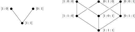
Figure 3. The projective line ${\mathbb{P}}^{1}_{k}$ and the projective plane ${\mathbb{P}}^{2}_{k}$ over $k$

4.2.2. Closed subschemes of projective space

The closed subschemes of the ordered blue projective $n$-space ${\mathbb{P}}^{n}_{B}$ over an ordered blueprint $B$ correspond to quotients of the free $B$-algebra $B[T_{0},\dotsc,T_{n}]$ by homogeneous relations, as we will explain in the following.

A homogeneous relation on $B[T_{0},\dotsc,T_{n}]$ is a relation of the form $\sum a_{i}\leqslant\sum b_{j}$ where $a_{i},b_{j}\in B_{k}$ are homogeneous of the same degree $k$. If $S$ is a set of homogeneous relations, then the quotient map $B[T_{0},\dotsc,T_{n}]\to B[T_{0},\dotsc,T_{n}]\!\sslash\!\langle S\rangle$ is a surjective morphism of graded $B$-algebras. For such morphisms, the following holds true.

Lemma 4.14.

Let $f:B[T_{0},\dotsc,T_{n}]\to C$ be a surjective morphism of graded $B$-algebras. Then $f^{\ast}:\operatorname{Proj}C\to{\mathbb{P}}^{n}_{B}$ is a closed immersion of ordered blue schemes.

Proof.

Let us write $D=B[T_{0},\dotsc,T_{n}]$ and $\myvarphi=f^{\ast}$ for short. The property of $f$ being a closed immersion can be tested on the open affine covering of ${\mathbb{P}}^{n}_{B}$ by $U_{i}=\operatorname{Spec}D[T_{i}^{-1}]_{0}$. The inverse image $\myvarphi^{-1}(U_{i})$ is the principal open $U_{h_{i}}\simeq\operatorname{Spec}C[h_{i}^{-1}]_{0}$ of $\operatorname{Proj}C$ where $h_{i}=f(T_{i})$. Thus $\myvarphi$ is affine. The induced morphisms $f_{i}:C[h_{i}^{-1}]_{0}\to D[T_{i}^{-1}]_{0}$ are surjective since $f$ is. This shows that $\myvarphi$ is a closed immersion. ∎

Remark 4.15.

The converse of Lemma 4.14 holds true as well, i.e. every closed $B$-subscheme of ${\mathbb{P}}^{n}_{B}$ comes from a surjective morphism of graded $B$-algebras. This can be proven as in the case of usual schemes.

4.3. Invertible sheaves

Loosely speaking, an invertible sheaf on an ordered blue scheme $X$ is a sheaf that is locally isomorphic to the structure sheaf ${\mathcal{O}}_{X}$ of $X$. To give this definition a precise meaning, we need to introduce ordered blue modules.

4.3.1. Ordered blue modules

An ordered semigroup is a commutative and unital semigroup $(M,+)$ together with a partial order $\leqslant$ that is compatible with the addition, i.e. $m\leqslant n$ and $p\leqslant q$ implies $m+p\leqslant n+q$. An ordered blue module is an ordered semigroup $M^{+}$ with neutral element $0$ together with a subset $M^{\bullet}$ that contains $0$ and generates $M^{+}$ as a semigroup. We write $M=(M^{\bullet},M^{+},\leqslant)$ for an ordered blue module. A morphism of ordered blue modules is an order preserving homomorphism $f:M^{+}\to N^{+}$ of semigroups with $f(0)=0$ and $f(M^{\bullet})\subset N^{\bullet}$. We denote the category of ordered blue modules by $\operatorname{OBMod}$.

Let $B$ be an ordered blueprint. An ordered blue $B$-module is a map $B^{+}\times M^{+}\to M^{+}$ that maps $(a,m)$ to $a.m$ and which satisfies, for all $a,b\in B$ and $m,n\in M$:

1. $a.m\in M^{\bullet}$ if $a\in B^{\bullet}$ and $m\in M^{\bullet}$;

2. $0.m=0$, $1.m=m$ and $a.0=0$;

3. $(ab).m=a.(b.m)$, $(a+b).m=a.m+b.m$ and $a.(m+n)=a.m+a.n$;

4. $a.m\leqslant b.n$ if $a\leqslant b$ and $m\leqslant n$.

A morphism of ordered blue $B$-modules is a morphism $f:M\to N$ of ordered blue modules such that the resulting diagram

commutes. We denote the category of ordered blue $B$-modules by $\operatorname{OBMod}B$.

Note that every ordered blue module has a unique structure as an ${{\mathbb{F}}_{1}}$-module. Thus $\operatorname{OBMod}$ is equivalent to $\operatorname{OBMod}{{\mathbb{F}}_{1}}$.

We remark that the category $\operatorname{OBMod}B$ is complete and cocomplete for every ordered blueprint $B$. In particular, the categorical product of $M$ and $N$ is the Cartesian product $M\times N$.

4.3.2. ${\mathcal{O}}_{X}$-modules

Let $X$ be an ordered blue scheme. A sheaf of ordered blue modules on $X$ is a sheaf on $X$ with values in $\operatorname{OBMod}$. For example, the structure sheaf ${\mathcal{O}}_{X}$ is naturally a sheaf of ordered blue modules. Note that products of sheaves in ordered blue modules are calculated valuewise in $\operatorname{OBMod}$.

An ${\mathcal{O}}_{X}$-module is a sheaf ${\mathcal{F}}$ on $X$ with values in $\operatorname{OBMod}$ together with a morphism of sheaves ${\mathcal{O}}_{X}\times{\mathcal{F}}\to{\mathcal{F}}$ such that for every open subset $U$ of $X$, the map ${\mathcal{O}}_{X}(U)\times{\mathcal{F}}(U)\to{\mathcal{F}}(U)$ endows ${\mathcal{F}}(U)$ with the structure of an ordered blue module. A morphism ${\mathcal{F}}\to{\mathcal{G}}$ of ${\mathcal{O}}_{X}$-modules is a morphism of sheaves ${\mathcal{F}}\to{\mathcal{G}}$ such that ${\mathcal{F}}(U)\to{\mathcal{G}}(U)$ is a morphism of ${\mathcal{O}}_{X}(U)$-modules for every open subset $U$ of $X$.

An invertible sheaf on $X$ is an ${\mathcal{O}}_{X}$-module ${\mathcal{L}}$ such that there are an open covering $\{U_{i}\}_{i\in I}$ and isomorphisms ${\mathcal{L}}|_{U_{i}}\to{\mathcal{O}}_{U_{i}}$ of ${\mathcal{O}}_{U_{i}}$-modules for every $i\in I$.

Example 4.16.

Recall that a principal open subset $U_{h}$ of ${\mathbb{P}}^{n}_{B}$ consists of all homogeneous prime ideals ${\mathfrak{p}}$ of $B[T_{0},\dotsc,T_{n}]$ not containing a given element $h$ nor the ideal $(T_{0},\dotsc,T_{n})$. The twisted sheaf ${\mathcal{O}}(d)$ on ${\mathbb{P}}^{n}_{B}$ is defined by ${\mathcal{O}}(d)(U_{h})=B[T_{0},\dotsc,T_{n}][h^{-1}]_{d}$, together with the tautological inclusions ${\mathcal{O}}(d)(U_{h})\to{\mathcal{O}}(d)(U_{g})$ whenever $U_{g}\subset U_{h}$, i.e. $g$ divides $h$. This definition extends uniquely to a sheaf on ${\mathbb{P}}^{n}_{B}$.

The sheaf ${\mathcal{O}}(d)$ inherits the structure of an ${\mathcal{O}}_{X}$-module from the natural action of ${\mathcal{O}}_{{\mathbb{P}}^{n}_{B}}(U_{h})=B[T_{0},\dotsc,T_{n}][h^{-1}]_{0}$ on ${\mathcal{O}}(d)(U_{h})=B[T_{0},\dotsc,T_{n}][h^{-1}]_{d}$ by multiplication. For the canonical open subsets $U_{i}=U_{T_{i}}$, multiplication by $T_{i}^{-d}$ yields an isomorphism ${\mathcal{O}}(d)(U_{i})\to{\mathcal{O}}_{{\mathbb{P}}^{n}_{B}}(U_{i})$, which shows that ${\mathcal{O}}(d)$ is an invertible sheaf.

Note that ${\mathcal{O}}(d)$ contains nontrivial global sections if and only if $d\geqslant 0$. For instance, $\Gamma{\mathcal{O}}(1)$ is freely generated over $B$ by the global sections $T_{0},\dotsc,T_{n}$.

4.3.3. Tensor products of invertible sheaves

As for usual schemes, there is a notion of a tensor product ${\mathcal{L}}\otimes{\mathcal{L}}^{\prime}={\mathcal{L}}\otimes_{{\mathcal{O}}_{X}}{\mathcal{L}}^{\prime}$ of invertible sheaves, which is again an invertible sheaf; it is defined as the sheafification of the presheaf $U\mapsto{\mathcal{L}}(U)\otimes_{{\mathcal{O}}_{X}(U)}{\mathcal{L}}^{\prime}(U)$. The dual ${\mathcal{L}}^{\vee}=\operatorname{Hom}({\mathcal{L}},{\mathcal{O}}_{X})$ of an invertible sheaf is an invertible sheaf, and ${\mathcal{L}}\otimes{\mathcal{L}}^{\vee}\simeq{\mathcal{O}}_{X}$. This turns the set $\operatorname{Pic}X$ of isomorphism classes of invertible sheaves on $X$ into an abelian group with respect to tensor product.

For example, if $B$ is an ordered blue field, $\operatorname{Pic}{\mathbb{P}}^{n}_{B}$ is an infinite cyclic group generated by the isomorphism class of ${\mathcal{O}}(1)$.

Note that two global sections $s\in\Gamma(X,{\mathcal{L}})$ and $s^{\prime}\in\Gamma(X,{\mathcal{L}}^{\prime})$ have a product $ss^{\prime}=s\otimes s^{\prime}$ in $\Gamma(X,{\mathcal{L}}\otimes{\mathcal{L}}^{\prime})$.

4.3.4. Pullbacks of invertible sheaves

Let $\myvarphi:X\to Y$ be a morphism of ordered blue schemes and ${\mathcal{L}}$ an invertible sheaf on $Y$. Let $\myvarphi^{-1}({\mathcal{L}})$ be the sheaf on $X$ that sends an open subset $U$ of $X$ to $\operatorname{colim}{\mathcal{L}}(V)$ where $V$ runs through all open subsets of $Y$ containing $\myvarphi(U)$. The pullback of ${\mathcal{L}}$ along $\myvarphi$ is the sheaf $\myvarphi^{\ast}({\mathcal{L}})=\myvarphi^{-1}({\mathcal{L}})\otimes_{\myvarphi^{-1}({\mathcal{O}}_{Y})}{\mathcal{O}}_{X}$ on $X$.

The pullback $\myvarphi^{\ast}({\mathcal{L}})$ of ${\mathcal{L}}$ is again an invertible sheaf, as can be seen as follows. Let $\{V_{i}\}$ be an open covering of $Y$ such that there are isomorphisms $\myeta_{i}:{\mathcal{L}}|_{V_{i}}\to{\mathcal{O}}_{V_{i}}$. Then $X$ is covered by the open subsets $U_{i}=\myvarphi^{-1}(V_{i})$ and ${\mathcal{O}}_{U_{i}}\simeq\myvarphi^{\ast}({\mathcal{O}}_{V_{i}})$ Thus the pullbacks of the $\myeta_{i}$ define isomorphisms $\myvarphi^{\ast}(\myeta_{i}):\myvarphi^{\ast}({\mathcal{L}})|_{U_{i}}\to{\mathcal{O}}_{U_{i}}$, which verifies that $\myvarphi^{\ast}({\mathcal{L}})$ is an invertible sheaf.

There is a natural morphism

$$\myvarphi^{\#}_{\mathcal{L}}:\ \Gamma(Y,{\mathcal{L}})\ \longrightarrow\ \Gamma\big{(}X,\myvarphi^{\ast}({\mathcal{L}})\big{)}$$

that sends a global section $s$ of ${\mathcal{L}}$ to $\big{(}\operatorname{colim}\textup{res}_{X,V}(s)\big{)}\otimes 1$, where the colimit taken over the system of all restrictions of $s$ to open subsets $V$ of $Y$ containing $\myvarphi(X)$.

The pullback commutes with tensor products, i.e. we have $\myvarphi^{\ast}({\mathcal{L}})\otimes\myvarphi^{\ast}({\mathcal{L}}^{\prime})\simeq\myvarphi^{\ast}({\mathcal{L}}\otimes{\mathcal{L}}^{\prime})$. As a result, we obtain a group homomorphism $\myvarphi^{\ast}:\operatorname{Pic}Y\to\operatorname{Pic}X$.

4.4. Morphisms to projective space

A key point in our approach to matroid bundles is the characterization of morphisms into projective space, which can be described in complete analogy to classical algebraic geometry. We will prove the relevant results in this section.

Let $X$ be an ordered blue scheme and ${\mathcal{L}}$ an invertible sheaf on $X$. Let $k={\mathcal{O}}_{X}(X)$ be the ordered blueprint of global sections of $X$. We denote the ordered blue $k$-module of global sections of ${\mathcal{L}}$ by $\Gamma{\mathcal{L}}={\mathcal{L}}(X)$. We say that global sections $s_{1},\dotsc,s_{n}\in\Gamma{\mathcal{L}}$ generate ${\mathcal{L}}$ if for every point $x\in X$ their images $s_{1,x},\dotsc,s_{n,x}$ in ${\mathcal{L}}_{x}$ generate ${\mathcal{L}}_{x}$ as an ordered blue ${\mathcal{O}}_{X,x}$-module. This is the case if and only if not all of $s_{1,x},\dotsc,s_{n,x}$ are contained in ${\mathfrak{m}}_{x}{\mathcal{L}}_{x}$, where ${\mathfrak{m}}_{x}$ is the maximal ideal of ${\mathcal{O}}_{x,x}$.

Example 4.17.

Let ${\mathcal{O}}(1)$ be the twisted sheaf on ${\mathbb{P}}^{n}_{B}$, cf. Example 4.16. Then the global sections $T_{0},\dotsc,T_{n}\in\Gamma{\mathcal{O}}(1)$ generate ${\mathcal{O}}(1)$, since ${\mathbb{P}}^{n}_{B}=\operatorname{Proj}B[T_{0},\dotsc,T_{n}]$ consists of all homogeneous prime $m$-ideals ${\mathfrak{p}}$ of $B[T_{0},\dotsc,T_{n}]$ that do not contain all of $T_{0},\dotsc,T_{n}$. Thus for every such ${\mathfrak{p}}$, there is at least one $T_{i}$ that is a unit in the stalk ${\mathcal{O}}(1)_{\mathfrak{p}}$.

Lemma 4.18.

Let $\myvarphi:X\to Y$ be a morphism of ordered blue schemes and ${\mathcal{L}}$ an invertible sheaf on $Y$ that is generated by global sections $s_{1},\dotsc,s_{n}\in\Gamma{\mathcal{L}}$. Then the images $\myvarphi^{\#}_{\mathcal{L}}(s_{1}),\dotsc,\myvarphi^{\#}_{\mathcal{L}}(s_{n})$ generate the invertible sheaf $\myvarphi^{\ast}{\mathcal{L}}$.

Proof.

As a first step, we observe that for every $x\in X$ and $y=\myvarphi(x)$,

$$(\myvarphi^{\ast}{\mathcal{L}})_{x}\ =\ \operatorname{colim}\myvarphi^{\ast}({\mathcal{L}})(U)\ =\ \operatorname{colim}\big{(}{\mathcal{L}}\otimes_{{\mathcal{O}}_{Y}}\myvarphi_{\ast}{\mathcal{O}}_{X}\big{)}(V)\ =\ \big{(}{\mathcal{L}}\otimes_{{\mathcal{O}}_{Y}}\myvarphi_{\ast}{\mathcal{O}}_{X}\big{)}_{y}\ =\ {\mathcal{L}}_{y}\otimes_{{\mathcal{O}}_{Y,y}}{\mathcal{O}}_{X,x}$$

where the first colimit is taken over all open neighbourhoods $U$ of $x$ and the second colimit is taken over all open neighbourhoods $V$ of $y$.

If we write $t_{i}=\myvarphi^{\#}_{\mathcal{L}}(s_{i})$ for $i=1,\dotsc,n$, the above calculation shows that we can identify the image $t_{i,x}$ of $t_{i}$ in the stalk $(\myvarphi^{\ast}{\mathcal{L}})_{x}={\mathcal{L}}_{y}\otimes_{{\mathcal{O}}_{Y,y}}{\mathcal{O}}_{X,x}$ with $s_{i,y}\otimes 1$ for $i=1,\dotsc,n$. From this, it is clear that if $s_{1,y},\dotsc,s_{n,y}$ generate ${\mathcal{L}}_{y}$ as an ordered blue ${\mathcal{O}}_{Y,y}$-module, then $s_{1,y}\otimes 1,\dotsc,s_{n,y}\otimes 1$ generate ${\mathcal{L}}_{y}\otimes_{{\mathcal{O}}_{Y,y}}{\mathcal{O}}_{X,x}$ as an ordered blue ${\mathcal{O}}_{X,x}$-module. We conclude that $t_{1},\dotsc,t_{n}$ generate $\myvarphi^{\ast}{\mathcal{L}}$. ∎

Lemma 4.19.

Let $X$ be an ordered blue scheme and $s\in\Gamma{\mathcal{O}}_{X}$. If the image $s_{x}$ of $s$ in ${\mathcal{O}}_{X,x}$ is a unit for all $x\in X$, then $s$ is a unit of $\Gamma{\mathcal{O}}_{X}$.

Proof.

Since ${\mathcal{O}}_{X,x}$ is the colimit over the local sections in the open neighbourhoods $U$ of $x$, an inverse $t_{x}$ of $s_{x}$ in ${\mathcal{O}}_{X,x}$ must come from an inverse of the restriction of $s$ to some open neighbourhood $U$ of $x$. Thus we find an open covering $U_{i}$ of $X$ such that the restrictions $s_{i}$ of $s$ to $U_{i}$ have inverses $t_{i}$ in $\Gamma{\mathcal{O}}_{U_{i}}$. On the intersections $U_{i}\cap U_{j}$, we get $\bar{t}_{i}=\bar{t}_{i}\,\bar{s}\,\bar{t}_{j}=\bar{t}_{j}$ where $\bar{t}_{i}$, $\bar{t}_{j}$ and $\bar{s}$ denote the respective restrictions of $t_{i}$, $t_{j}$ and $s$ to $U_{i}\cap U_{j}$. This shows that the local sections $t_{i}$ coincide on the overlaps of the $U_{i}$ and thus glue to a global section $t$ of ${\mathcal{O}}_{X}$. Since $st$ is locally equal to $1$, we must have $st=1$ in $\Gamma{\mathcal{O}}_{X}$, which shows that $s$ is a unit in $\Gamma{\mathcal{O}}_{X}$. ∎

Theorem 4.20.

Let $B$ be an ordered blueprint, $X$ an ordered blue $B$-scheme and $n\geqslant 0$. Let ${\mathbb{P}}^{n}_{B}=\operatorname{Proj}B[x_{0},\dotsc,x_{n}]$ be the projective space over $B$ and ${\mathcal{O}}(1)$ the twisted sheaf of degree $1$.

1. If $\myvarphi:X\to{\mathbb{P}}_{B}^{n}$ is a $B$-linear morphism, then $\myvarphi^{\ast}\big{(}{\mathcal{O}}(1)\big{)}$ is an invertible sheaf on $X$, which is generated by the global sections $s_{i}=\myvarphi^{\#}_{{\mathcal{O}}(1)}(x_{i})$ for $i=0,\dotsc,n$.

2. If ${\mathcal{L}}$ is an invertible sheaf on $X$ and $s_{0},\dotsc,s_{n}\in\Gamma{\mathcal{L}}$ are global sections that generate ${\mathcal{L}}$, there is a unique $B$-linear morphism $\myvarphi:X\to{\mathbb{P}}^{n}_{B}$ such that there is an isomorphism ${\mathcal{L}}\to\myvarphi^{\ast}\big{(}{\mathcal{O}}(1)\big{)}$ that identifies $s_{i}$ with $\myvarphi^{\#}_{{\mathcal{O}}(1)}(x_{i})$ for $i=0,\dotsc,n$.

Proof.

Part (1) of the theorem follows immediately from Lemma 4.18.

Part (2) is trivial for the empty scheme $X$. Thus we may assume that $X$ is nonempty. Then the subsets $X_{i}=\{\,x\in X\,|\,s_{i}\in{\mathcal{L}}_{x}^{\times}\,\}$ are open, and they cover $X$ since $s_{0},\dotsc,s_{n}$ generate ${\mathcal{L}}$.

Since ${\mathcal{L}}$ is locally free of rank $1$, we can choose for every $x\in X$ a generator $\mytheta_{x}$ of ${\mathcal{L}}_{x}$ as an ${\mathcal{O}}_{X,x}$-module. Thus for every $i=0,\dotsc,n$ and $x\in X$, the image $s_{i,x}$ of $s_{i}$ in ${\mathcal{L}}_{x}$ is a multiple of $\mytheta_{x}$, i.e. $s_{i,x}=\mylambda_{i,x}\mytheta_{x}$ for some $\mylambda_{i,x}$.

For a fixed $i$, we have $s_{i}\in{\mathcal{L}}_{x}^{\times}$ for every $x\in X_{i}$. Lemma 4.19 implies that the restriction of $s_{i}$ to $X_{i}$ is invertible. Thus we can define for every $j$ the quotient $\frac{s_{j}}{s_{i}}$ in $\Gamma X_{i}$. Note that $\frac{s_{j}}{s_{i}}$ does not depend on the choice of the generators $\mytheta_{x}$.

Let $U_{i}=\operatorname{Spec}B[\frac{x_{0}}{x_{i}},\dotsc,\frac{x_{n}}{x_{i}}]$ be the $i$-th canonical open subset of ${\mathbb{P}}^{n}_{B}$. The association $\frac{x_{j}}{x_{i}}\mapsto\frac{s_{j}}{s_{i}}$ defines a morphism $f_{i}:B[\frac{x_{0}}{x_{i}},\dotsc,\frac{x_{n}}{x_{i}}]\to\Gamma X_{i}$. By Lemma 4.8, $f_{i}$ corresponds to a morphism $\myvarphi_{i}:X_{i}\to U_{i}$ of ordered blue schemes, which is obviously $B$-linear. Since $\myvarphi_{i}$ and $\myvarphi_{j}$ coincide on the intersection $X_{i}\cap X_{j}$, the morphisms $\myvarphi_{i}$ glue to a $B$-linear morphism $\myvarphi:X\to{\mathbb{P}}_{B}^{n}$.

It is clear from the definition of $\myvarphi$ that $\myvarphi^{\ast}\big{(}{\mathcal{O}}(1)\big{)}$ is isomorphic to ${\mathcal{L}}$ and that the pullbacks of the coordinates $x_{i}$ coincide with the global sections $s_{i}$. It is also clear that there is a unique $\myvarphi$ with these properties. This finishes the proof of the theorem. ∎

Let $X$ be an ordered blue scheme. An invertible sheaf with $n$ generators is an invertible sheaf ${\mathcal{L}}$ together with global sections $s_{1},\dotsc,s_{n}$ that generate ${\mathcal{L}}$. Two invertible sheaves with $n$ generators $({\mathcal{L}};s_{1},\dotsc,s_{n})$ and $({\mathcal{L}}^{\prime};s_{1}^{\prime},\dotsc,s_{n}^{\prime})$ are isomorphic if there exists an isomorphism $\myvarphi:{\mathcal{L}}\to{\mathcal{L}}^{\prime}$ of invertible sheaves such that $s_{i}=\myvarphi^{\#}_{\mathcal{L}}(s_{i}^{\prime})$ for $i=1,\dotsc,n$. Let $\operatorname{PicGen}(n,X)$ be the set of isomorphism classes of invertible sheaves on $X$ with $n$ generators.

The following is an immediate consequence of Theorem 4.20.

Corollary 4.21.

Let $B$ be an ordered blueprint, $X$ an ordered blue $B$-scheme and $n\geqslant 0$. Then the map

$$\begin{array}[]{ccc}\operatorname{Hom}_{B}(X,{\mathbb{P}}^{n}_{B})&\longrightarrow&\operatorname{PicGen}(n+1,X)\\ \myvarphi:X\to{\mathbb{P}}^{n}_{B}&\longmapsto&\big{(}\myvarphi^{\ast}\big{(}{\mathcal{O}}(1)\big{)};\myvarphi^{\#}_{{\mathcal{O}}(1)}(x_{0}),\dotsc,\myvarphi^{\#}_{{\mathcal{O}}(1)}(x_{n})\big{)}\end{array}$$

is a bijection. In particular, we have ${\mathbb{P}}^{n}_{B}(C)=\operatorname{PicGen}(n+1,X)$ if $X=\operatorname{Spec}C$. ∎

5. Families of matroids and their moduli spaces

At this point, we have developed the necessary formalism to define matroid bundles over ordered blue ${{\mathbb{F}}_{1}^{\pm}}$-schemes. Besides our immediate goal of constructing a (fine) moduli space of matroids, which requires the notion of a universal family, the concept of a matroid bundle should have applications to tropical geometry (and conceivably to classical matroid theory as well). For example, we hope that matroid bundles will be useful for developing a theory of sheaf cohomology for tropical varieties. In addition, a suitable notion of families of valuated matroids appears to be a necessary ingredient for defining families of tropical schemes in the sense of Maclagan and Rincón ([40]).

In this section, we will introduce matroid bundles, study their first properties, and use them to define a suitable moduli functor which will be represented by the moduli space of matroids.

5.1. Families of matroids

An ordered blue ${{\mathbb{F}}_{1}^{\pm}}$-scheme is an ordered blue scheme $X$ together with a structure morphism $X\to\operatorname{Spec}{{\mathbb{F}}_{1}^{\pm}}$. An ${{\mathbb{F}}_{1}^{\pm}}$-linear morphism between two ordered blue ${{\mathbb{F}}_{1}^{\pm}}$-schemes is a morphism $\myvarphi:X\to Y$ that commutes with the respective structure morphisms. This defines the category $\operatorname{Sch}_{{\mathbb{F}}_{1}^{\pm}}$ of ordred blue ${{\mathbb{F}}_{1}^{\pm}}$-schemes.

If $X$ is an ordered blue ${{\mathbb{F}}_{1}^{\pm}}$-scheme, then $\Gamma(X,{\mathcal{O}}_{X})$ is an ${{\mathbb{F}}_{1}^{\pm}}$-algebra. As usual, we denote the weak inverse of $1$ by $\myepsilon$. Note that $\Gamma(X,{\mathcal{L}})$ is an ordered blue $\Gamma(X,{\mathcal{O}}_{X})$-module for every invertible sheaf ${\mathcal{L}}$ over $X$. We define ${\mathcal{L}}^{\otimes 2}={\mathcal{L}}\otimes{\mathcal{L}}$ and recall from section 4.3.3 that the product $s\cdot s^{\prime}$ of two elements $s,s^{\prime}\in\Gamma(X,{\mathcal{L}})$ is an element of $\Gamma(X,{\mathcal{L}}^{\otimes 2})$.

Definition 5.1.

Let $E$ be a non-empty finite ordered set, $r$ a natural number and $X$ an ordered blue ${{\mathbb{F}}_{1}^{\pm}}$-scheme. A Grassmann-Plücker function of rank $r$ on $E$ over $X$ is an invertible sheaf ${\mathcal{L}}$ over $X$ together with a map

$$\begin{array}[]{cccc}\Delta:&\binom{E}{r}&\longrightarrow&\Gamma(X,{\mathcal{L}})\\ &I&\longmapsto&\Delta(I)\end{array}$$

such that $\{\Delta(I)\}_{I\in\binom{E}{r}}$ generate ${\mathcal{L}}$ and satisfy the Plücker relations

$$0\quad\leqslant\quad\sum_{k=1}^{r+1}\ \myepsilon^{k}\ \cdot\ \Delta({I\cup\{i_{k}\}})\ \cdot\ \Delta({I^{\prime}-\{i_{k}\}})$$

in $\Gamma(X,{\mathcal{L}}^{\otimes 2})$ for every $(r-1)$-subset $I$ and every $(r+1)$-subset $I^{\prime}=\{i_{1},\dotsc,i_{r+1}\}$ of $E$, where $i_{1}<\dotsb<i_{r+1}$ and we define $\Delta({I\cup\{i_{k}\}})=0$ if $I\cup\{i_{k}\}$ is of cardinality $r-1$.

Two Grassmann-Plücker functions $({\mathcal{L}},\Delta)$ and $({\mathcal{L}}^{\prime},\Delta^{\prime})$ on $X$ are isomorphic if there exists an isomorphism $\myvarphi:{\mathcal{L}}\to{\mathcal{L}}^{\prime}$ of invertible sheaves such that $\Delta^{\prime}=\Gamma\myvarphi\circ\Delta$, where $\Gamma\myvarphi:\Gamma(X,{\mathcal{L}})\to\Gamma(X,{\mathcal{L}}^{\prime})$ is the induced isomorphism between the ordered blueprints of global sections.

A matroid bundle over $X$ is an isomorphism class of Grassmann-Plücker functions.

5.1.1. Pullbacks of matroid bundles

The pullback $\myvarphi^{\ast}({\mathcal{M}})$ of a matroid bundle ${\mathcal{M}}$ on $Y$ along a morphism $\myvarphi:X\to Y$ of ordered blue ${{\mathbb{F}}_{1}^{\pm}}$-schemes is defined by the following lemma.

Lemma 5.2.

Let $\myvarphi:X\to Y$ be a morphism in $\operatorname{OBSch}_{{\mathbb{F}}_{1}^{\pm}}$ and ${\mathcal{L}}$ an invertible sheaf on $Y$. Let $E$ be a non-empty finite ordered set, $r$ a natural number and ${\mathcal{M}}$ a matroid bundle over $Y$ represented by a Grassmann-Plücker function $\Delta:\binom{E}{r}\to\Gamma(Y,{\mathcal{L}})$. Then $\myvarphi^{\ast}(\Delta)=\myvarphi_{\mathcal{L}}^{\#}\circ\Delta:\binom{E}{r}\to\Gamma(X,\myvarphi^{\ast}({\mathcal{L}}))$ is a Grassmann-Plücker function over $X$ and the matroid bundle $\myvarphi^{\ast}({\mathcal{M}})=[\tilde{\Delta}]$ over $X$ does not depend on the choice of representative $\Delta$ of ${\mathcal{M}}$.

Proof.

As a first step, we verify that $\myvarphi^{\ast}(\Delta)=\myvarphi_{\mathcal{L}}^{\#}\circ\Delta$ is a Grassmann-Plücker function. Since $\{\Delta(I)\}_{I\in\binom{E}{r}}$ generates ${\mathcal{L}}$, Lemma 4.18 implies that $\{\myvarphi^{\#}_{\mathcal{L}}(\Delta(I))\}_{I\in\binom{E}{r}}$ generates $\myvarphi^{\ast}({\mathcal{L}})$. The identification $\myvarphi^{\ast}({\mathcal{L}}^{\otimes 2})=\myvarphi^{\ast}({\mathcal{L}})^{\otimes 2}$ yields a morphism $\myvarphi^{\#}_{{\mathcal{L}}^{\otimes 2}}:\Gamma(Y,{\mathcal{L}}^{\otimes 2})\to\Gamma(X,\myvarphi^{\ast}({\mathcal{L}})^{\otimes 2})$ of ordered blueprints. Thus the validity of the Plücker relations in $\Gamma(Y,{\mathcal{L}}^{\otimes 2})$ implies the validity of the Plücker relations in $\Gamma(X,\myvarphi^{\ast}({\mathcal{L}})^{\otimes 2})$. This shows that $\myvarphi^{\ast}(\Delta)$ is a Grassmann-Plücker function.

Next we show independence from the choice of representative $\Delta$. Let $\Delta^{\prime}:\binom{E}{r}\to\Gamma(Y,{\mathcal{L}}^{\prime})$ be another Grassmann-Plücker function representing ${\mathcal{M}}$, i.e. there is an isomorphism $\myeta:{\mathcal{L}}\to{\mathcal{L}}^{\prime}$ such that $\Delta^{\prime}=\Gamma(Y,\myeta)\circ\Delta$. This yields an isomorphism $\myvarphi^{\ast}(\myeta):\myvarphi^{\ast}({\mathcal{L}})\to\myvarphi^{\ast}({\mathcal{L}}^{\prime})$ and $\myvarphi^{\ast}(\Delta^{\prime})=\Gamma(Y,\myvarphi^{\ast}(\myeta))\circ\myvarphi^{\ast}(\Delta)$, as desired. ∎

5.2. The moduli functor of matroids

Let $E$ be a non-empty finite ordered set and $r$ a natural number. We extend the functor $\operatorname{\mathpzc{Mat}}(r,E):\operatorname{{OBlpr}}_{{\mathbb{F}}_{1}^{\pm}}\to\operatorname{Sets}$ to the functor

$$\begin{array}[]{cccc}\operatorname{\mathpzc{Mat}}(r,E):&\operatorname{OBSch}_{{\mathbb{F}}_{1}^{\pm}}&\longrightarrow&\operatorname{Sets}\\[5.0pt] &X&\longmapsto&\big{\{}\,\text{matroid bundles of rank $r$ on $E$ over $X$}\,\big{\}}\\[5.0pt] &\myvarphi:X\to Y&\longmapsto&\myvarphi^{\ast}:\operatorname{\mathpzc{Mat}}(r,E)(Y)\to\operatorname{\mathpzc{Mat}}(r,E)(X)\end{array}$$

Thanks to Proposition 5.3, we have $\operatorname{\mathpzc{Mat}}(r,E)(\operatorname{Spec}B)=\operatorname{\mathpzc{Mat}}(r,E)(B)$ for every ${{\mathbb{F}}_{1}^{\pm}}$-algebra and $\operatorname{\mathpzc{Mat}}(r,E)(\operatorname{Spec}f)=\operatorname{\mathpzc{Mat}}(r,E)(f)$ for every morphism $f:B\to C$ in $\operatorname{{OBlpr}}_{{\mathbb{F}}_{1}^{\pm}}$.

5.3. Compatibility with matroids over ordered blueprints

In the following, we verify that matroid bundles over $\operatorname{Spec}B$ correspond bijectively to $B$-matroids in a functorial way.

Proposition 5.3.

Let $B$ be an ${{\mathbb{F}}_{1}^{\pm}}$-algebra, $E$ a non-empty finite ordered set, $r$ a natural number and $X=\operatorname{Spec}B$. Then the map

$$\begin{array}[]{cccc}\Phi_{B}:&\big{\{}\text{$B$-matroids of rank $r$ on $E$}\big{\}}&\longrightarrow&\big{\{}\text{matroid bundles of rank $r$ on $E$ over $X$}\big{\}}\\[5.0pt] &M=[\Delta:\binom{E}{r}\to B]&\longmapsto&\widetilde{M}=[\myiota_{B}\circ\Delta:\binom{E}{r}\to\Gamma(X,{\mathcal{O}}_{X})]\end{array}$$

is a bijection, where $\myiota_{B}:B\to\Gamma(X,{\mathcal{O}}_{X})$ is the inclusion as constant sections. If $f:B\to C$ is a morphism of ${{\mathbb{F}}_{1}^{\pm}}$-algebras, $\myvarphi=f^{\ast}:\operatorname{Spec}C\to\operatorname{Spec}B$ the induced morphism and $M$ a $B$-matroid, then $\Phi_{C}(f_{\ast}(M))=\myvarphi^{\ast}(\Phi_{B}(M))$. In other words, we have a commutative diagram of functors

Proof.

To begin with, we verify that $\Phi_{B}$ is well-defined. Let $\Delta:\binom{E}{r}\to B$ be a Grassmann-Plücker function. Then $\Delta(I)\in B^{\times}$ for some $r$-subset $I$ of $E$. Therefore $\myiota_{B}(\Delta(I))\in\Gamma(X,{\mathcal{O}}_{X})^{\times}$, which shows that $\{\myiota_{B}\circ\Delta(I)\}_{I\in\binom{E}{r}}$ generates ${\mathcal{O}}_{X}$. The Plücker relations for $\Delta$ imply the Plücker relations for $\myiota_{B}\circ\Delta$. Thus $\myiota_{B}\circ\Delta$ is a Grassmann-Plücker function over $X$. Since every $a\in B^{\times}$ defines an automorphism of ${\mathcal{O}}_{X}$, the map $\Phi_{B}$ is independent of the choice of representative, which shows that $\Phi_{B}$ is well-defined.

The injectivity of $\Phi_{B}$ can be verified as follows. The inclusion $\myiota_{B}:B\to\Gamma(X,{\mathcal{O}}_{X})$ as constant sections is an isomorphism of ordered blueprints, which implies that any two Grassmann-Plücker functions $\Delta,\Delta^{\prime}:\binom{E}{r}\to B$ are different if $\myiota_{B}\circ\Delta$ and $\myiota_{B}\circ\Delta^{\prime}$ are different. Moreover, this implies that the automorphisms of ${\mathcal{O}}_{X}$ are equal to the automorphisms of $B$ as a $B$-module, which are given by multiplication with a unit, i.e. $\operatorname{Aut}({\mathcal{O}}_{X})=B^{\times}$. Thus different $B$-matroids yield different matroid bundles over $X$, which proves the injectivity of $\Phi_{B}$.

The surjectivity of $\Phi_{B}$ can be verified as follows. It is obvious if $B$ is trivial. If $B$ is nontrivial, then $B$ has a unique maximal ideal, which is ${\mathfrak{m}}=B-B^{\times}$. Therefore the only open subset of $X$ containing ${\mathfrak{m}}$ is $X$ itself. Thus there are no nontrivial coverings of $X$ and consequently every invertible sheaf on $X$ is isomorphic to ${\mathcal{O}}_{X}$. This shows that we can represent every matroid bundle ${\mathcal{M}}$ over $X$ by a Grassmann-Plücker function $\tilde{\Delta}:\binom{E}{r}\to\Gamma(X,{\mathcal{O}}_{X})$. Composing $\tilde{\Delta}$ with the inverse $\myiota_{B}^{-1}$ of $\myiota_{B}$ yields a map $\Delta=\myiota_{B}^{-1}\circ\tilde{\Delta}:\binom{E}{r}\to B$. Since $\{\myiota_{B}\circ\Delta(I)\}_{I\in\binom{E}{r}}$ generates ${\mathcal{O}}_{X}$, it generates the stalk ${\mathcal{O}}_{X,{\mathfrak{m}}}=B$ as an ordered blue $B$-module, which means that $\Delta(I)\in B^{\times}$ for some $r$-subset $I$ of $E$. The Plücker relations for $\tilde{\Delta}$ imply the Plücker relations for $\Delta$. Thus $\Delta$ is a Grassmann-Plücker function with coefficients in $B$ and $\tilde{\Delta}=\Phi_{B}(\Delta)$, as desired. This shows that $\Phi_{B}$ is bijective.

To verify the final claim of the proposition, let $\Delta:\binom{E}{r}\to B$ be a Grassmann-Plücker function representing $M$. Then $f_{\ast}(M)$ is represented by the Grassmann-Plücker function $f\circ\Delta:\binom{E}{r}\to C$. The matroid bundle $\widetilde{M}=\Phi_{B}(M)$ is represented by the Grassmann-Plücker function $\myiota_{B}\circ\Delta:\binom{E}{r}\to\Gamma(X,{\mathcal{O}}_{X})$. By Lemma 5.2, the pullback $\myvarphi^{\ast}(\widetilde{M})$ is represented by the Grassmann-Plücker function $\myvarphi_{{\mathcal{O}}_{X}}^{\#}\circ\myiota_{B}\circ\Delta:\binom{E}{r}\to\Gamma(Y,\myvarphi^{\ast}({\mathcal{O}}_{Y}))$ where $Y=\operatorname{Spec}C$.

The result now follows from the commutativity of the diagram

where $\myiota_{C}:C\to\Gamma(Y,{\mathcal{O}}_{Y})$ is the canonical isomorphism. ∎

5.3.1. Example of a matroid bundle over the projective line over ${\mathbb{K}}$

In this example, we investigate matroid bundles of rank $2$ on $E=\{1,2,3,4\}$ over the projective line ${\mathbb{P}}^{1}_{\mathbb{K}}=\operatorname{Proj}\big{(}{\mathbb{K}}[T_{0},T_{1}]\big{)}$. We review some general facts that we will use below.

Since ${\mathbb{K}}^{\bullet}=\{0,1\}$, the underlying monoid of ${\mathbb{K}}[T_{0},T_{1}]$ is $\{0\}\cup\{T_{0}^{e_{0}}T_{1}^{e_{1}}|e_{0},e_{1}\in{\mathbb{N}}\}$. Thus the homogeneous prime ideals of ${\mathbb{K}}[T_{0},T_{1}]$ not containing both $T_{0}$ and $T_{1}$ are $(0)$, $(T_{0})$ and $(T_{1})$, cf. Figure 3 for an illustration.

As in the classical case, every invertible sheaf on ${\mathbb{P}}^{1}_{\mathbb{K}}$ is isomorphic to a twisted sheaf ${\mathcal{O}}(d)$ for some $d\in{\mathbb{Z}}$ and every automorphism of ${\mathcal{O}}(d)$ is given by the multiplication by a unit of ${\mathbb{K}}$, i.e. $\operatorname{Aut}({\mathcal{O}}(d))={\mathbb{K}}^{\times}=\{1\}$. This means that every matroid bundle ${\mathcal{M}}$ of rank $2$ on $E$ over ${\mathbb{P}}^{1}_{\mathbb{K}}$ is represented by a unique Grassmann-Plücker function of the form $\Delta:\binom{E}{2}\to\Gamma(X,{\mathcal{O}}(d))$. Note that there is only one Plücker relation in this case, which is

$$0\ \leqslant\ \Delta_{1,2}\Delta_{3,4}\ +\ \Delta_{1,3}\Delta_{2,4}\ +\ \Delta_{1,4}\Delta_{2,3}$$

where we write $\Delta_{i,j}=\Delta(\{i,j\})$.

We have $\Gamma({\mathbb{P}}^{1}_{\mathbb{K}},{\mathcal{O}}(d))=\{0\}$ for $d<0$, which means that ${\mathcal{O}}(d)$ cannot be generated by global sections for $d<0$. For $d\geqslant 0$, we have $\Gamma({\mathbb{P}}^{1}_{\mathbb{K}},{\mathcal{O}}(d))=\{0\}\cup\{T_{0}^{d},T_{0}^{d-1}T_{1},\dotsc,T_{1}^{d}\}$. Since $T_{0}$ is contained in the maximal ideal of ${\mathbb{K}}[T_{0},T_{1}]_{(T_{0})}$ and $T_{1}$ is contained in the maximal ideal of ${\mathbb{K}}[T_{0},T_{1}]_{(T_{1})}$, there is a unique minimal set of global sections that generates ${\mathcal{O}}(d)$: for $d=0$, this set is $\{1\}$ and for $d>0$, this set is $\{T_{0}^{d},T_{1}^{d}\}$.

For every $d\geqslant 0$, there is exists a nonempty set of Grassmann-Plücker functions $\Delta:\binom{E}{2}\to\Gamma({\mathbb{P}}^{1}_{\mathbb{K}},{\mathcal{O}}(d))$. We classify them for $d=0$ and $d=1$ in the following.

The case $d=0$ ties to ${\mathbb{K}}$-matroids as follows: the pullback along the structure morphism $\mychi:{\mathbb{P}}^{1}_{\mathbb{K}}\to\operatorname{Spec}{\mathbb{K}}$ yields a bijection

$$\textstyle\mychi^{\ast}:\quad\left\{\begin{array}[]{c}\text{Grassmann-Pl\"{u}cker functions}\\ \Delta:\binom{E}{2}\to{\mathbb{K}}\end{array}\right\}\quad\longrightarrow\quad\left\{\begin{array}[]{c}\text{Grassmann-Pl\"{u}cker functions}\\ \Delta:\binom{E}{2}\to\Gamma({\mathbb{P}}^{1}_{\mathbb{K}},{\mathcal{O}}_{{\mathbb{P}}^{1}_{\mathbb{K}}})\end{array}\right\},$$

which realizes ${\mathbb{K}}$-matroids as “constant” matroid bundles over ${\mathbb{P}}^{1}_{\mathbb{K}}$. The inverse is given by the pullback $\myxi^{\ast}(\Delta)$ along an arbitrary morphism $\myxi:\operatorname{Spec}{\mathbb{K}}\to{\mathbb{P}}^{1}_{\mathbb{K}}$. (Note that there are three such morphisms, which are characterized by their image, which can be each of the three points of ${\mathbb{P}}^{1}_{\mathbb{K}}$.)

The ${\mathbb{K}}$-matroids of rank $2$ on $E$ correspond to the functions $\Delta:\binom{E}{2}\to\{0,1\}$ for which at least two of the products $\Delta_{1,2}\Delta_{3,4}$, $\Delta_{1,3}\Delta_{2,4}$ and $\Delta_{1,4}\Delta_{2,3}$ are equal to $1$, or for which all three products are equal to $0$ but $\Delta_{i,j}=1$ for at least one $2$-subset $\{i,j\}$ of $E$.

The case $d=1$ is more involved and reveals some novel phenomena. We have $\Gamma({\mathbb{P}}^{1}_{\mathbb{K}},{\mathcal{O}}(1))=\{0,T_{0},T_{1}\}$. Let $\Delta:\binom{E}{2}\to\{0,T_{0},T_{1}\}$ be a function. Since $\{\Delta_{i,j}\}_{\{i,j\}\in\binom{E}{2}}$ has to generate ${\mathcal{O}}(1)$ in order for $\Delta$ to be a Grassmann-Plücker function, we must have $\Delta_{i,j}=T_{0}$ and $\Delta_{k,l}=T_{1}$ for some $2$-subsets $\{i,j\}$ and $\{k,l\}$ of $E$. Moreover, at least two of the products $\Delta_{1,2}\Delta_{3,4}$, $\Delta_{1,3}\Delta_{2,4}$ and $\Delta_{1,4}\Delta_{2,3}$ must be equal to each other, while the third might be equal to the other two or equal to $0$. This allows for the following Grassmann-Plücker functions:

• $\Delta_{1,2}\Delta_{3,4}=\Delta_{1,3}\Delta_{2,4}=\Delta_{1,4}\Delta_{2,3}=T_{0}T_{1}$;

• $\Delta_{i,j}\Delta_{k,l}=\Delta_{i,k}\Delta_{j,l}=T_{0}^{2}$, $\Delta_{i,l}=0$, and $\Delta_{j,k}=T_{1}$ for some $\{i,j,k,l\}=E$;

• $\Delta_{i,j}\Delta_{k,l}=\Delta_{i,k}\Delta_{j,l}=T_{1}^{2}$, $\Delta_{i,l}=0$, and $\Delta_{j,k}=T_{0}$ for some $\{i,j,k,l\}=E$;

• $\Delta_{i,j}\Delta_{k,l}=\Delta_{i,k}\Delta_{j,l}=T_{0}T_{1}$, $\Delta_{i,l}=0$, and $\Delta_{j,k}\in\{0,T_{0},T_{1}\}$ for some $\{i,j,k,l\}=E$;

• $\Delta_{1,2}\Delta_{3,4}=\Delta_{1,3}\Delta_{2,4}=\Delta_{1,4}\Delta_{2,3}=0$, $\Delta_{i,j}=T_{0}$, and $\Delta_{i,k}=T_{1}$ for some pairwise distinct $i,j,k$.

The cases $d\geqslant 2$ become increasingly more involved.

5.4. The moduli space of matroids

We define the matroid space of rank $r$ on $E$ as the ordered blue scheme

$$\textstyle\operatorname{Mat}(r,E)\quad=\quad\operatorname{Proj}\Big{(}\,{{\mathbb{F}}_{1}^{\pm}}\big{[}\,x_{I}\,\big{|}\,I\in\binom{E}{r}\,\big{]}\!\sslash\!\operatorname{\mathpzc{Pl}}(r,E)\,\Big{)},$$

where $\operatorname{\mathpzc{Pl}}(r,E)$ is generated by the Plücker relations

$$0\quad\leqslant\quad\sum_{k=1}^{r+1}\ \myepsilon^{k}\ \cdot\ x_{I\cup\{i_{k}\}}\ \cdot\ x_{I^{\prime}-\{i_{k}\}}$$

for every $(r-1)$-subset $I$ and every $(r+1)$-subset $I^{\prime}=\{i_{1},\dotsc,i_{r+1}\}$ of $E$. By definition, it comes with a closed immersion into projective space

$$\textstyle\myiota:\ \operatorname{Mat}(r,n)\ \longrightarrow\ {\mathbb{P}}^{N}_{{{\mathbb{F}}_{1}^{\pm}}}\ =\ \operatorname{Proj}\Big{(}\,{{\mathbb{F}}_{1}^{\pm}}\big{[}\,x_{I}\,\big{|}\,I\in\binom{E}{r}\,\big{]}\,\Big{)}$$

where $N=\#\binom{E}{r}-1$. We denote the pullback of the tautological bundle ${\mathcal{O}}(1)$ of ${\mathbb{P}}^{N}_{{{\mathbb{F}}_{1}^{\pm}}}$ to $\operatorname{Mat}(r,E)$ by ${\mathcal{L}}_{\textup{univ}}=\myiota^{\ast}{\mathcal{O}}(1)$. The pullbacks of the canonical sections $x_{I}$ of ${\mathcal{O}}(1)$ define a map

$$\begin{array}[]{cccc}\Delta_{\textup{univ}}:&\binom{E}{r}&\longrightarrow&\Gamma(\operatorname{Mat}(r,E),{\mathcal{L}}_{\textup{univ}}).\\ &I&\longmapsto&\Delta_{\textup{univ}}(I)=\myiota^{\#}_{{\mathcal{O}}(1)}(x_{I})\end{array}$$

Since $\{x_{I}\}_{I\in\binom{E}{r}}$ generates ${\mathcal{O}}(1)$, Lemma 4.18 implies that $\{\Delta_{\textup{univ}}(I)\}_{I\in\binom{E}{r}}$ generates ${\mathcal{L}}_{\textup{univ}}$. Since $\operatorname{Mat}(r,E)$ satisfies the Plücker relations, the function $\Delta_{\textup{univ}}$ is a Grassmann-Plücker function on $\operatorname{Mat}(r,E)$. The universal matroid bundle is the class ${\mathcal{M}}_{\textup{univ}}$ of $\Delta_{\textup{univ}}$, which is a matroid bundle of rank $r$ on $E$ over $\operatorname{Mat}(r,E)$.

Remark 5.4.

The matroid space $\operatorname{Mat}(r,E)$ should be thought of as an analogue of the Grassmannian $\operatorname{Gr}(r,E)_{R}$ over a ring $R$ from usual algebraic geometry. In fact, we can recover the Grassmannian as the scheme $\operatorname{Mat}(r,E)_{B}^{+}$ associated to the base extension $\operatorname{Mat}(r,E)_{B}$ of the matroid space to the ordered blueprint $B$ associated with $R$. The functor $(-)^{+}$ respects many of the standard ‘decorations’ of the Grassmannian (e.g. its Plücker embedding into ${\mathbb{P}}^{N}$) in an obvious sense, linking them to their respective avatars in classical algebraic geometry.

The following theorem shows that the pair $(\operatorname{Mat}(r,E),{\mathcal{M}}_{\textup{univ}})$ represents the moduli functor $\operatorname{\mathpzc{Mat}}(r,E)$:

Theorem 5.5.

Let $E$ be a non-empty finite ordered set and let $r$ be a natural number. The ordered blue ${{\mathbb{F}}_{1}^{\pm}}$-scheme $\operatorname{Mat}(r,E)$, together with its universal matroid bundle ${\mathcal{M}}_{\textup{univ}}$, is the fine moduli space of all matroid bundles of rank $r$ on $E$, i.e. the map

$$\begin{array}[]{cccc}\Phi:&\operatorname{Hom}_{{{\mathbb{F}}_{1}^{\pm}}}\big{(}X,\operatorname{Mat}(r,E)\big{)}&\longrightarrow&\operatorname{\mathpzc{Mat}}(r,E)(X)\\[5.0pt] &\myvarphi:X\to\operatorname{Mat}(r,E)&\longmapsto&\myvarphi^{\ast}({\mathcal{M}}_{\textup{univ}})\\[5.0pt] \end{array}$$

is a bijection for every ordered blue ${{\mathbb{F}}_{1}^{\pm}}$-scheme $X$.

Proof.

Note that every morphism $\myvarphi:\operatorname{Spec}B\to\operatorname{Mat}(r,E)$ is automatically ${{\mathbb{F}}_{1}^{\pm}}$-linear since the morphism ${{\mathbb{F}}_{1}^{\pm}}\to B$ is unique. Therefore we can omit ${{\mathbb{F}}_{1}^{\pm}}$-linearity from the notation for the morphism set $\operatorname{Hom}(X,\operatorname{Mat}(r,E))$.

As a first step, we define a map $\Psi:\operatorname{\mathpzc{Mat}}(r,E)(X)\to\operatorname{Hom}(X,\operatorname{Mat}(r,E))$ in the opposite direction of $\Phi$. Let ${\mathcal{M}}$ be a matroid bundle over $X$ that is represented by a Grassmann-Plücker function $\Delta:\binom{E}{r}\to\Gamma(X,{\mathcal{L}})$ for some invertible sheaf ${\mathcal{L}}$ over $X$. Let $N=\#\binom{E}{r}-1$. By Theorem 4.20 (2), there is a unique ${{\mathbb{F}}_{1}^{\pm}}$-linear morphism $\myvarphi_{0}:X\to{\mathbb{P}}_{{{\mathbb{F}}_{1}^{\pm}}}^{N}$ such that $\Delta(I)=\myvarphi^{\#}_{0}(x_{I})$ for all $I\in\binom{E}{r}$. Since $\Delta$ satisfies the Plücker relations, $\myvarphi_{0}$ factors uniquely into a morphism $\myvarphi:X\to\operatorname{Mat}(r,E)$ followed by the closed immersion $\myiota:\operatorname{Mat}(r,E)\to{\mathbb{P}}_{{{\mathbb{F}}_{1}^{\pm}}}^{N}$.

That $\Phi$ and $\Psi$ are mutually inverse bijections follows at once from Corollary 4.21.

Consider a morphism $\mypsi:Y\to X$ in $\operatorname{OBSch}_{{\mathbb{F}}_{1}^{\pm}}$. Then by the definition of the pullback of a matroid bundle, we have $(\myvarphi\circ\mypsi)^{\ast}({\mathcal{M}}_{\textup{univ}})=\mypsi^{\ast}(\myvarphi^{\ast}({\mathcal{M}}_{\textup{univ}}))$, which establishes the functoriality of the bijection $\Phi$. This completes the proof of the theorem. ∎

5.5. Duality

One of the fundamental features of matroid theory is that every matroid (with coefficients) comes with a canonical dual matroid. This extends to matroid bundles, and, in fact, the duality is derived from a duality between the moduli spaces.

Theorem 5.6.

Let $E$ be a non-empty finite ordered set, $r\leqslant\#E$ a natural number and $r^{{\mbox{\larger[-8]$\vee$}}}=\#E-r$. Let $I^{c}=E-I$ denote the complement of a subset $I$ of $E$. Then the association $x_{I}\mapsto x_{I^{c}}$ defines a graded ${{\mathbb{F}}_{1}^{\pm}}$-linear isomorphism

$$\textstyle\myalpha^{\mbox{\larger[-8]$\vee$}}:\ {{\mathbb{F}}_{1}^{\pm}}\big{[}\,x_{I}\,\big{|}\,I\in\binom{E}{r}\,\big{]}\!\sslash\!\operatorname{\mathpzc{Pl}}(r,E)\quad\stackrel{{\scriptstyle\sim}}{{\longrightarrow}}\quad{{\mathbb{F}}_{1}^{\pm}}\big{[}\,x_{I}\,\big{|}\,I\in\binom{E}{r^{\mbox{\larger[-8]$\vee$}}}\,\big{]}\!\sslash\!\operatorname{\mathpzc{Pl}}(r^{\mbox{\larger[-8]$\vee$}},E)$$

and thus an isomorphism

$$\myvarphi^{\mbox{\larger[-8]$\vee$}}:\ \operatorname{Mat}(r^{\mbox{\larger[-8]$\vee$}},E)\ \stackrel{{\scriptstyle\sim}}{{\longrightarrow}}\ \operatorname{Mat}(r,E)$$

of ordered blue ${{\mathbb{F}}_{1}^{\pm}}$-schemes.

Proof.

Clearly $x_{I}\mapsto x_{I^{c}}$ defines a graded ${{\mathbb{F}}_{1}^{\pm}}$-linear isomorphism

$$\textstyle\tilde{\myalpha}^{\mbox{\larger[-8]$\vee$}}:\ {{\mathbb{F}}_{1}^{\pm}}\big{[}\,x_{I}\,\big{|}\,I\in\binom{E}{r}\,\big{]}\ \stackrel{{\scriptstyle\sim}}{{\longrightarrow}}\ {{\mathbb{F}}_{1}^{\pm}}\big{[}\,x_{I}\,\big{|}\,I\in\binom{E}{r^{\mbox{\larger[-8]$\vee$}}}\,\big{]}.$$

Thus we are left with verifying that $\tilde{\myalpha}^{\mbox{\larger[-8]$\vee$}}$ preserves the respective Plücker relations.

For this verification, we rewrite the Plücker relations in a form that is more symmetric with respect to duality. For $I\subset E$ and $i\in E$, we define $\mysigma(i,I)=\#\{j\in I|j\leqslant i\}$. Then the Plücker relation given by an $(r-1)$-subset $I$ and an $(r+1)$-subset $J$ of $E$ is

$$0\quad\leqslant\quad\sum_{i\in J-I}\ \myepsilon^{\mysigma(i,I)+\mysigma(i,J)}\ \cdot\ x_{I\cup\{i\}}\ \cdot\ x_{J-\{i\}}.$$

Note that

$$(I\cup\{i\})^{c}=I^{c}-\{i\},\quad(J-\{i\})^{c}=J^{c}\cup\{i\}\quad\text{and}\quad J-I=I^{c}-J^{c}.$$

The last equality implies that $\mysigma(i,J-I)=\mysigma(i,I^{c}-J^{c})$. Since $\mysigma(i,J-I)=\mysigma(i,J)-\mysigma(i,I\cap J)$, and likewise for $\mysigma(i,I^{c}-J^{c})$, we obtain

$$\mysigma(i,J)-\mysigma(i,I\cap J)\ =\ \mysigma(i,I^{c})-\mysigma(i,J^{c}\cap I^{c}).$$

Exchanging the roles of $I$ and $J$ yields an analogous equation. Adding both equations yields

$$\mysigma(i,I)+\mysigma(i,J)-2\mysigma(i,I\cap J)\ =\ \mysigma(i,J^{c})+\mysigma(i,I^{c})-2\mysigma(i,J^{c}\cap I^{c}).$$

This shows that $\myepsilon^{\mysigma(i,J^{c})+\mysigma(i,I^{c})}=\myepsilon^{\mysigma(i,I)+\mysigma(i,J)}$. Thus applying $\tilde{\myalpha}^{\mbox{\larger[-8]$\vee$}}$ to the Plücker relation for $I$ and $J$ yields

$$0\quad\leqslant\quad\sum_{i\in I^{c}-J^{c}}\ \myepsilon^{\mysigma(i,J^{c})+\mysigma(i,I^{c})}\ \cdot\ x_{J^{c}\cup\{i\}}\ \cdot\ x_{I^{c}-\{i\}},$$

which is the Plücker relation for the $(r^{\mbox{\larger[-8]$\vee$}}-1)$-subset $J^{c}$ and the $(r^{\mbox{\larger[-8]$\vee$}}+1)$-subset $I^{c}$ of $E$. We conclude that $\tilde{\myalpha}^{\mbox{\larger[-8]$\vee$}}$ maps $\operatorname{\mathpzc{Pl}}(r,E)$ to $\operatorname{\mathpzc{Pl}}(r^{\mbox{\larger[-8]$\vee$}},E)$, which completes the proof of the theorem. ∎

Definition 5.7.

Let $X$ be an ordered blue ${{\mathbb{F}}_{1}^{\pm}}$-scheme endowed with an involution (generalizing the involution on a tract $F$ from Section 3.1.4) $\myiota:X\to X$, ${\mathcal{L}}$ a line bundle on $X$, and ${\mathcal{M}}$ a matroid bundle on $X$ that is represented by the Grassmann-Plücker function $\Delta:\binom{E}{r}\to\Gamma(X,{\mathcal{L}})$. The dual of $\Delta$ with respect to $\myiota$ is the function

$$\textstyle\begin{array}[]{cccc}\Delta_{\myiota}^{\mbox{\larger[-8]$\vee$}}:&\binom{E}{r^{\mbox{\larger[-8]$\vee$}}}&\longrightarrow&\Gamma(X,{\mathcal{L}})\\ &I&\longmapsto&\myiota_{\mathcal{L}}^{\#}\circ\Delta(I^{c})\end{array}$$

where $\myiota_{\mathcal{L}}^{\#}:\Gamma(X,{\mathcal{L}})\to\Gamma(X,{\mathcal{L}})$ is the involution induced by $\myiota$.

The dual of ${\mathcal{M}}$ with respect to $\myiota$ is the isomorphism class ${\mathcal{M}}_{\myiota}^{\mbox{\larger[-8]$\vee$}}$ of $\Delta_{\myiota}^{\mbox{\larger[-8]$\vee$}}$.

In the following proposition, we verify that $\Delta_{\myiota}^{\mbox{\larger[-8]$\vee$}}$ is a Grassmann-Plücker function and thus that ${\mathcal{M}}_{\myiota}^{\mbox{\larger[-8]$\vee$}}$ is a matroid bundle on $X$. Moreover, we will see that the duality of matroid bundles is compatible with the duality of the moduli spaces of matroids from Theorem 5.6.

Note that in case that $X=\operatorname{Spec}F$ for an idyll $F$, the duality of the matroid bundle ${\mathcal{M}}$ on $\operatorname{Spec}F$ coincides with the duality of the corresponding $F^{\textup{tract}}$-matroid $M$ from [4, Thm. 2.24].

Given a matroid bundle ${\mathcal{M}}$ on $X$, we call the morphism $\mychi_{\mathcal{M}}:X\to\operatorname{Mat}(r,E)$ that corresponds to ${\mathcal{M}}$ under the bijection from Theorem 5.5 the characteristic morphism of ${\mathcal{M}}$.

Proposition 5.8.

Let $X$ be an ordered blue ${{\mathbb{F}}_{1}^{\pm}}$-scheme with involution $\myiota:X\to X$ and ${\mathcal{L}}$ a line bundle on $X$. Let $\Delta:\binom{E}{r}\to\Gamma(X,{\mathcal{L}})$ be a Grassmann-Plücker function that represents a matroid bundle ${\mathcal{M}}$ on $X$ with characteristic morphism $\mychi_{\mathcal{M}}:X\to\operatorname{Mat}(r,E)$. Then the dual $\Delta_{\myiota}^{\mbox{\larger[-8]$\vee$}}$ of $\Delta$ with respect to $\myiota$ is a Grassmann-Plücker function and ${\mathcal{M}}_{\myiota}^{\mbox{\larger[-8]$\vee$}}$ is the matroid bundle on $X$ whose characteristic morphism is

$$\mychi_{{\mathcal{M}}_{\myiota}^{\mbox{\larger[-8]$\vee$}}}\ =\ \myvarphi^{\mbox{\larger[-8]$\vee$}}\circ\mychi_{\mathcal{M}}\circ\myiota:\ X\ \stackrel{{\scriptstyle\myiota}}{{\longrightarrow}}\ X\ \stackrel{{\scriptstyle\mychi_{\mathcal{M}}}}{{\longrightarrow}}\ \operatorname{Mat}(r,E)\ \stackrel{{\scriptstyle\myvarphi^{\mbox{\larger[-8]$\vee$}}}}{{\longrightarrow}}\ \operatorname{Mat}(r^{\mbox{\larger[-8]$\vee$}},E)$$

where $r^{\mbox{\larger[-8]$\vee$}}=\#E-r$ and $\myvarphi^{\mbox{\larger[-8]$\vee$}}$ is the isomorphism from Theorem 5.6.

Proof.

That $\Delta_{\myiota}^{\mbox{\larger[-8]$\vee$}}$ is a Grassmann-Plücker function can be shown directly by an analogous calculation to that from the proof of Theorem 5.6. Alternatively, we can show this by applying the result from Theorem 5.6 in the following way.

The direct sum $\bigoplus_{i\geqslant 0}\Gamma(X,{\mathcal{L}}^{\otimes i})$ can be given the structure of an ordered blueprint $(B^{\bullet},B^{+},\leqslant)$ as follows:

• The ambient semiring $B^{+}$ is the direct sum of the semigroups $\Gamma(X,{\mathcal{L}}^{\otimes i})^{+}$ for all $i\geqslant 0$, which comes with a natural multiplication.

• The monoid $B^{\bullet}$ is the union of all the subsets $\Gamma(X,{\mathcal{L}}^{\otimes i})^{\bullet}$ in $B^{+}$.

• The partial order $\leqslant$ is the smallest additive and multiplicative partial order that contains the partial order of $\Gamma(X,{\mathcal{L}}^{\otimes i})^{+}$ for every $i\geqslant 0$.

Since $\Delta$ is a Grassmann-Plücker function, the association $x_{I}\mapsto\Delta(I)$ defines a morphism

$$\textstyle\myxi_{\Delta}:\ {{\mathbb{F}}_{1}^{\pm}}\big{[}\,x_{I}\,\big{|}\,I\in\binom{E}{r}\,\big{]}\!\sslash\!\operatorname{\mathpzc{Pl}}(r,E)\ \longrightarrow\ \bigoplus_{i\geqslant 0}\Gamma(X,{\mathcal{L}}^{\otimes i}).$$

Composing this morphism with the map $j_{r,E}:\binom{E}{r}\to{{\mathbb{F}}_{1}^{\pm}}\big{[}x_{I}\big{|}I\in\binom{E}{r}\big{]}\!\sslash\!\operatorname{\mathpzc{Pl}}(r,E)$ that sends $I$ to $x_{I}$ gives the Grassmann-Plücker function $\Delta:\binom{E}{r}\to\Gamma(X,{\mathcal{L}})$, where we consider $\Gamma(X,{\mathcal{L}})$ as a subset of $\bigoplus_{i\geqslant 0}\Gamma(X,{\mathcal{L}}^{\otimes i})$.

Precomposing $\myxi_{\Delta}$ with the inverse of the isomorphism $\myalpha^{\mbox{\larger[-8]$\vee$}}$ from Theorem 5.6 yields a morphism $\myxi_{\Delta_{\myiota}^{\mbox{\larger[-8]$\vee$}}}$, whose composition with $j_{r^{\mbox{\larger[-8]$\vee$}},E}$ is the dual $\Delta_{\myiota}^{\mbox{\larger[-8]$\vee$}}$ of $\Delta$. This means that we obtain a commutative diagram

Since $\Delta_{\myiota}^{\mbox{\larger[-8]$\vee$}}$ factors through $\myxi_{\Delta_{\myiota}^{\mbox{\larger[-8]$\vee$}}}$, it satisfies the Plücker relations. Thus $\Delta_{\myiota}^{\mbox{\larger[-8]$\vee$}}$ is a Grassmann-Plücker function, which verifies the first part of the proposition.

Note that the characteristic morphism $\mychi_{\mathcal{M}}:X\to\operatorname{Mat}(r,E)$ is induced from the graded morphism $\myxi_{\Delta}$. Thus applying the $\operatorname{Proj}$-functor to inner square of the above diagram yields a commutative diagram

which verifies the second part of the proposition. ∎

5.6. Contraction and deletion

The operations of contracting and deleting an element $e$ of the ground set $E$ of an $F$-matroid $M$, as introduced in [4, section 3.9], are defined on the level of maps between subvarieties of the matroid spaces for $E$ and $E^{\prime}=E-\{e\}$ and appropriate ranks. To this end we define the closed subschemes

$$\textstyle V_{/e}\ =\ \operatorname{Proj}\Big{(}{{\mathbb{F}}_{1}^{\pm}}[T_{I}\mid I\in\binom{E}{r}]\!\sslash\!\langle\operatorname{\mathpzc{Pl}}(r,E)\cup\{T_{I}\mid e\in I\}\rangle\Big{)}$$

and

$$\textstyle V_{\backslash e}\ =\ \operatorname{Proj}\Big{(}{{\mathbb{F}}_{1}^{\pm}}[T_{I}\mid I\in\binom{E}{r}]\!\sslash\!\langle\operatorname{\mathpzc{Pl}}(r,E)\cup\{T_{I}\mid e\notin I\}\rangle\Big{)}$$

of $\operatorname{Mat}(r,E)$, as well as their respective set-theoretic complements

$$U_{/e}\ =\ \operatorname{Mat}(r,E)-V_{/e}\qquad\text{and}\qquad U_{\backslash e}\ =\ \operatorname{Mat}(r,E)-V_{\backslash e},$$

which we consider as open subschemes of $\operatorname{Mat}(r,E)$.

The graded morphism

$$\begin{array}[]{ccc}{{\mathbb{F}}_{1}^{\pm}}[T_{J}\mid J\in\binom{E^{\prime}}{r-1}]\!\sslash\!\operatorname{\mathpzc{Pl}}(r-1,E^{\prime})&\longrightarrow&{{\mathbb{F}}_{1}^{\pm}}[T_{I}\mid I\in\binom{E}{r}]\!\sslash\!\operatorname{\mathpzc{Pl}}(r,E)\\ T_{J}&\longmapsto&T_{J\cup\{e\}}\end{array}$$

defines a rational map $\operatorname{Mat}(r,E)\;\leavevmode\hbox to15.94pt{\vbox to5.2pt{\text{[drawing]}}}\;\operatorname{Mat}(r-1,E^{\prime})$ whose domain is $U_{/e}$, since the inverse image of a homogeneous prime ideal $\langle T_{I}\mid I\in{\mathcal{I}}\rangle$ is relevant if and only if ${\mathcal{I}}$ contains an $I$ with $e\notin I$. This yields a morphism $\Psi^{o}_{/e}:U_{/e}\to\operatorname{Mat}(r-1,E^{\prime})$. The graded morphism

$$\begin{array}[]{ccc}{{\mathbb{F}}_{1}^{\pm}}[T_{J}\mid J\in\binom{E^{\prime}}{r}]\!\sslash\!\operatorname{\mathpzc{Pl}}(r,E^{\prime})&\longrightarrow&{{\mathbb{F}}_{1}^{\pm}}[T_{I}\mid I\in\binom{E}{r}]\!\sslash\!\langle\operatorname{\mathpzc{Pl}}(r,E)\cup\{T_{I}\mid e\in I\}\rangle\\ T_{J}&\longmapsto&T_{J}\end{array}$$

is an isomorphism and defines an isomorphism $\Psi^{c}_{/e}:V_{/e}\to\operatorname{Mat}(r,E^{\prime})$ of ordered blue schemes. Combining these morphisms, we obtain the diagram

$$\operatorname{Mat}(r,E)\ \stackrel{{\scriptstyle\myiota_{/e}}}{{\longleftarrow}}\ U_{/e}\,\myamalg\,V_{/e}\ \stackrel{{\scriptstyle\Psi_{/e}}}{{\longrightarrow}}\ \operatorname{Mat}(r-1,E^{\prime})\,\myamalg\,\operatorname{Mat}(r,E^{\prime}),$$

where $\myiota_{/e}$ is the disjoint union of the inclusions of the subschemes $U_{/e}$ and $V_{/e}$ into $\operatorname{Mat}(r,E)$ and $\Psi_{/e}$ is the disjoint union of $\Psi^{o}_{/e}$ and $\Psi^{c}_{/e}$.

Similarly, the graded morphism

$$\begin{array}[]{ccc}{{\mathbb{F}}_{1}^{\pm}}[T_{J}\mid J\in\binom{E^{\prime}}{r}]\!\sslash\!\operatorname{\mathpzc{Pl}}(r,E^{\prime})&\longrightarrow&{{\mathbb{F}}_{1}^{\pm}}[T_{I}\mid I\in\binom{E}{r}]\!\sslash\!\operatorname{\mathpzc{Pl}}(r,E)\\ T_{J}&\longmapsto&T_{J}\end{array}$$

and the graded isomorphism

$$\begin{array}[]{ccc}{{\mathbb{F}}_{1}^{\pm}}[T_{J}\mid J\in\binom{E^{\prime}}{r-1}]\!\sslash\!\operatorname{\mathpzc{Pl}}(r-1,E^{\prime})&\longrightarrow&{{\mathbb{F}}_{1}^{\pm}}[T_{I}\mid I\in\binom{E}{r}]\!\sslash\!\langle\operatorname{\mathpzc{Pl}}(r,E)\cup\{T_{I}\mid e\in I\}\rangle\\ T_{J}&\longmapsto&T_{J\cup\{e\}}\end{array}$$

define morphisms $\Psi^{o}_{\backslash e}:U_{\backslash e}\to\operatorname{Mat}(r,E^{\prime})$ and $\Psi^{c}_{\backslash e}:V_{\backslash e}\to\operatorname{Mat}(r-1,E^{\prime})$ of ordered blue schemes, and combining these yields the diagram

$$\operatorname{Mat}(r,E)\ \stackrel{{\scriptstyle\myiota_{\backslash e}}}{{\longleftarrow}}\ U_{\backslash e}\,\myamalg\,V_{\backslash e}\ \stackrel{{\scriptstyle\Psi_{\backslash e}}}{{\longrightarrow}}\ \operatorname{Mat}(r,E^{\prime})\,\myamalg\,\operatorname{Mat}(r-1,E^{\prime}).$$

The following theorem explains how these morphisms extend the usual operations of contraction and deletion to the level of moduli spaces. Since we will not use this result in the paper, we omit a proof.

Theorem 5.9.

Let $F$ be an idyll and $M$ an $F$-matroid of rank $r$ on $E$ with characteristic morphism $\mychi_{M}:\operatorname{Spec}F\to\operatorname{Mat}(r,E)$. Let $e\in E$ and $E^{\prime}=E-\{e\}$. Define $r_{/e}=r$ if $e$ is a loop and $r_{/e}=r-1$ if not, and define $r_{\backslash e}=r-1$ if $e$ is a coloop and $r_{\backslash e}=r$ if not. Let $\mychi_{M/e}:\operatorname{Spec}F\to\operatorname{Mat}(r_{/e},E^{\prime})$ and $\mychi_{M\backslash e}:\operatorname{Spec}F\to\operatorname{Mat}(r_{\backslash e},E^{\prime})$ be the characteristic morphisms of the contraction $M/e$ and the deletion $M\backslash e$, respectively. Then the following holds:

1. The morphism $\mychi_{M}$ factors into a uniquely determined morphism $\mychi_{M,/e}:\operatorname{Spec}F\to U_{/e}\myamalg V_{/e}$ composed with $\myiota_{/e}$, as well as into a uniquely determined morphism $\mychi_{M,\backslash e}:\operatorname{Spec}F\to U_{\backslash e}\myamalg V_{\backslash e}$ composed with $\myiota_{\backslash e}$.

2. The morphism $\mychi_{M\backslash e}$ is the unique morphism from $\operatorname{Spec}F$ to $\operatorname{Mat}(r_{/e},E^{\prime})$ that makes the diagram

   commute, and $\mychi_{M/e}$ is the unique morphism from $\operatorname{Spec}F$ to $\operatorname{Mat}(r_{\backslash e},E^{\prime})$ that makes the diagram

   commute, where the vertical arrows on the right hand side are the respective canonical inclusions into the coproduct.

3. Let $r^{\vee}=\#E-r$ and let $U_{\backslash e}^{\vee}$ and $V^{\vee}_{\backslash e}$ be the obvious respective variants of $U_{\backslash e}$ and $V_{\backslash e}$ for $\operatorname{Mat}(r^{\vee},E)$. Then there are unique isomorphisms $\myvarphi^{o,\vee}:U_{/e}\to U_{\backslash e}^{\vee}$ and $\myvarphi^{c,\vee}:V_{/e}\to V_{\backslash e}^{\vee}$ that make the diagram

   commute, where $\myiota_{\backslash e}^{\vee}$ and $\Psi_{\backslash e}^{\vee}$ are the obvious variants of $\myiota_{\backslash e}$ and $\Psi_{\backslash e}$, respectively, and where the vertical morphisms denoted by $\myvarphi^{\vee}$ are the isomorphisms from Theorem 5.6.

5.7. Rational point sets

In this section, we explain how the matroid space recovers classical objects like the Grassmannian, the Dressian and the MacPhersonian as rational point sets.

Let $B$ be an ${{\mathbb{F}}_{1}^{\pm}}$-algebra. By the universal property of the matroid space, $\operatorname{Mat}(r,E)(B)$ corresponds to the set of $B$-matroids of rank $r$ on $E$. If $B$ carries a topology, then $\operatorname{Mat}(r,E)(B)$ inherits the so-called fine topology from $B$. The fine topology is defined by a general categorical construction, which has been exhibited first in [39] and which has been transferred to rational point sets of ordered blue schemes in [36]. Instead of recalling the definition of the fine topology in full generality, we will provide an equivalent characterization in Theorem 5.11.

A topological idyll is an idyll $F$ together with a topology such that the multiplication $F\times F\to F$ (where $F\times F$ carries the product topology) is a continuous map, and such that $F^{\times}$ is an open subset of $F$ and the inversion map $F^{\times}\to F^{\times}$, sending $a$ to $a^{-1}$, is continuous.

Remark 5.10.

It might appear strange at first sight that the definition of a topological idyll does not involve any continuity condition for addition. Thus a topological idyll that is a field is not necessarily a topological field. However, our definition is guided by properties of the fine topology on rational point sets, as described in Theorem 5.11 below. The proof of these properties does not require any continuity conditions for addition, in contrast to the corresponding proof for topological fields. This difference in the proofs can be traced back to the fact that free algebras in the world of ordered blueprints consist of monomials (as opposed to more general polynomials).

Given an ordered blue scheme $X$ and a topological idyll $F$, the fine topology for the rational point set $X(F)$ is determined in terms of the following theorem.

Theorem 5.11.

Let $F$ be a topological idyll. Then there is a unique way to endow the rational point sets $X(F)$ for all ordered blue schemes $X$ with a topology such that the following properties hold true:

1. the canonical bijection $F\to{\mathbb{A}}_{F}^{1}(F)$ is a homeomorphism;

2. the canonical bijection $(X\times Y)(F)\to X(F)\times Y(F)$ is a homeomorphism;

3. for every morphism $Y\to X$, the canonical map $Y(F)\to X(F)$ is continuous;

4. for every open / closed immersion $Y\to X$, the canonical inclusion $Y(F)\to X(F)$ is an open / closed topological embedding;

5. for every covering of $X$ by ordered blue open subschemes $U_{i}$, a subset $W$ of $X(F)$ is open if and only if $W\cap U_{i}(F)$ is open in $U_{i}(F)$ for every $i$.

Moreover, if $F\to F^{\prime}$ is a continuous morphism of idylls and $X$ an ordered blue scheme, the induced map $X(F)\to X(F^{\prime})$ is continuous.

Proof.

This is a special case of Theorem 5.2 in [36]. ∎

Example 5.12.

Every topological field is a topological idyll in a tautological way. Anderson and Davis have extended this notion to hyperfields in [3]. It turns out that a topological hyperfield is the same as a topological idyll if identified with the associated idyll via the functor $(-)^{\textup{oblpr}}:\operatorname{{HypFields}}\to\operatorname{{OBlpr}}^{\pm}$. In the following, we consider the following topological idylls:

• the reals ${\mathbb{R}}$ with the usual topology;

• the Krasner hyperfield ${\mathbb{K}}$ together with the topology that consists of the open subsets $\emptyset$, $\{1\}$, ${\mathbb{K}}$;

• the sign hyperfield ${\mathbb{S}}$ together with the topology that consists of the open subsets $\emptyset$, $\{1\}$, $\{-1\}$, $\{\pm 1\}$, ${\mathbb{S}}$;

• the tropical hyperfield ${\mathbb{T}}$ together with the topology coming from the identification of ${\mathbb{T}}$ with ${\mathbb{R}}_{\geqslant 0}$ and its embedding into ${\mathbb{R}}$;

• the regular partial field ${{\mathbb{F}}_{1}^{\pm}}$ together with the topology that consists of the open subsets $\emptyset$, $\{1\}$, $\{-1\}$, $\{\pm 1\}$, ${{\mathbb{F}}_{1}^{\pm}}$.

Note that [3] contains reasons why it might be better to exclude all neighborhoods of $0$ in the topology of ${\mathbb{T}}$; we refer to section 2.3.2 of loc. cit., but ignore this issue in the following. The topological spaces $X(F)$ appearing in Theorem 5.11 are also closely related to Jun’s considerations in [26]. Namely for $F={\mathbb{K}}$, $F={\mathbb{T}}$ or $F={\mathbb{S}}$, a blue scheme $X$ and its associated scheme $X^{+}$, it is not hard to show that the topological space $X(F)$ coincides with the topological space $X^{+}(F)$ from [26].

5.7.1. Matroids

A matroid is the same as a ${\mathbb{K}}$-matroid where ${\mathbb{K}}=\{0,1\}\!\sslash\!\langle 0\leqslant 1+1,0\leqslant 1+1+1\rangle$ is the Krasner hyperfield. Thus $\operatorname{Mat}(r,E)({\mathbb{K}})$ is the set of all matroids of rank $r$ on $E$. The topology on ${\mathbb{K}}$ turns $\operatorname{Mat}(r,E)({\mathbb{K}})$ into a contractible topological space, cf. [3, section 6] for details.

5.7.2. Oriented matroids and the MacPhersonian

Note that as an idyll, the sign hyperfield turns into ${\mathbb{S}}=\{0,1,\myepsilon\}\!\sslash\!{\mathcal{R}}$ where ${\mathcal{R}}$ is generated by relations $0\leqslant 1+\dotsb+1+\myepsilon+\dotsb+\myepsilon$ that contain at least one $1$ and one $\myepsilon$.

An oriented matroid is the same thing as a ${\mathbb{S}}$-matroid. Thus $\operatorname{Mat}(r,E)({\mathbb{S}})$ is the set of all oriented matroids of rank $r$ on $E$. The topology of ${\mathbb{S}}$ turns $\operatorname{Mat}(r,E)({\mathbb{S}})$ into a topological space, which is, by definition, the MacPhersonian $\operatorname{MacPh}(r,E)$ of rank $r$ on $E$; cf. [3, section 6] for details.

5.7.3. Subspaces and the Grassmannian

Let $k$ be a field, which we identify with the idyll $k^{\bullet}\!\sslash\!\langle 0\leqslant\sum a_{i}|\sum a_{i}=0\text{ in }k\rangle$. (Note that this results from considering $k$ as a partial field and applying the functor $\operatorname{{PartFields}}\to\operatorname{{OBlpr}}^{\pm}$ or, equivalently, from considering $k$ as a hyperfield and applying the functor $\operatorname{{HypFields}}\to\operatorname{{OBlpr}}^{\pm}$. This allows us to consider fields as objects of either subcategory $\operatorname{{PartFields}}$ and $\operatorname{{HypFields}}$ of $\operatorname{{OBlpr}}^{\pm}$.)

It is immediate that the class of a Grassmann-Plücker function $\Delta:\binom{E}{r}\to k$ corresponds to the point $\big{[}\Delta(I)\big{|}I\in\binom{E}{r}\big{]}$ of the Grassmannian $\operatorname{Gr}(r,E)(k)$ and vice-versa. This yields an identification $\operatorname{Mat}(r,E)(k)=\operatorname{Gr}(r,E)(k)$ and shows that a $k$-matroid is the same thing as an $r$-dimensional subspace of $k^{E}$.

5.7.4. The oriented matroid of real subspaces

The topology of ${\mathbb{R}}$ endows $\operatorname{Mat}(r,E)({\mathbb{R}})$ with a topology that coincides with the usual topology of the real Grassmannian. The hyperfield morphism $\textup{sign}:{\mathbb{R}}\to{\mathbb{S}}$ is continuous and therefore induces a continuous map

$$\operatorname{Gr}(r,E)({\mathbb{R}})\ =\ \operatorname{Mat}(r,E)({\mathbb{R}})\ \longrightarrow\ \operatorname{Mat}(r,E)({\mathbb{S}})\ =\ \operatorname{MacPh}(r,E).$$

This map sends an $r$-dimensional subspace $V$ of ${\mathbb{R}}^{E}$ to its associated oriented matroid $M_{V}$, which is the class of the Grassmann Plücker function $\textup{sign}\circ\Delta:\binom{E}{r}\to{\mathbb{S}}$, where $\Delta$ is defined by the Plücker coordinates $\big{[}\Delta(I)\big{|}I\in\binom{E}{r}\big{]}$ of $V$.

This map is closely connected to the MacPhersonian conjecture, as formulated by Mnëv and Ziegler in [43], which asserts a relation between the homotopy type of $\operatorname{Gr}(r,E)({\mathbb{R}})$ and the MacPhersonian $\operatorname{MacPh}(r,E)$. For more details on these connections, see [3, section 7]. Note that certain cases of this conjecture have recently been disproven by Liu in [34].

5.7.5. Valuated matroids and the Dressian

A valuated matroid is the same thing as a ${\mathbb{T}}$-matroid, where ${\mathbb{T}}$ is the tropical hyperfield. Thus $\operatorname{Mat}(r,E)({\mathbb{T}})$ is the set of all valuated matroids of rank $r$ on $E$. An $r$-dimensional tropical linear space in ${\mathbb{R}}^{E}$ is the geometric realization of a valuated matroid as a subspace of ${\mathbb{R}}^{E}$, analogous to the Bergman fan of a matroid; cf. [53] for a precise definition. The Dressian $\operatorname{Dress}(r,E)$ is the set of $r$-dimensional tropical linear spaces in ${\mathbb{R}}^{E}$.

By definition, the $r$-dimensional tropical linear spaces in ${\mathbb{R}}^{E}$ correspond bijectively to the valuated matroids of rank $r$ on $E$. This yields an identification $\operatorname{Dress}(r,E)=\operatorname{Mat}(r,E)({\mathbb{T}})$ of the Dressian with the ${\mathbb{T}}$-rational points of the matroid space. Note that the topology of ${\mathbb{T}}$ endows the Dressian $\operatorname{Dress}(r,E)$ with a natural topology.

5.7.6. Regular matroids

It follows from our explanations in section 3.4.3 that the subset of regular matroids in $\operatorname{Mat}(r,E)({\mathbb{K}})$ is equal to the image of the map $\operatorname{Mat}(r,E)({{\mathbb{F}}_{1}^{\pm}})\to\operatorname{Mat}(r,E)({\mathbb{K}})$ induced by the unique morphism ${{\mathbb{F}}_{1}^{\pm}}\to{\mathbb{K}}$. Note that the topology of ${{\mathbb{F}}_{1}^{\pm}}$ endows the set of ${{\mathbb{F}}_{1}^{\pm}}$-matroids $\operatorname{Mat}(r,E)({{\mathbb{F}}_{1}^{\pm}})$ with a topology. Since the morphism ${{\mathbb{F}}_{1}^{\pm}}\to{\mathbb{K}}$ is continuous, the map $\operatorname{Mat}(r,E)({{\mathbb{F}}_{1}^{\pm}})\to\operatorname{Mat}(r,E)({\mathbb{K}})$ is continuous.

Note that this map is in general not injective, as the following example shows. Let $E=\{1,2\}$. Then the Grassmann-Plücker functions $\Delta_{1}:\binom{E}{1}\to{{\mathbb{F}}_{1}^{\pm}}$ and $\Delta_{2}:\binom{E}{1}\to{{\mathbb{F}}_{1}^{\pm}}$ with

$$\Delta_{1}(\{1\})\ =\ \Delta_{1}(\{2\})\ =\ \Delta_{2}(\{1\})=1\quad\text{and}\quad\Delta_{2}(\{2\})\ =\ \myepsilon$$

define different ${{\mathbb{F}}_{1}^{\pm}}$-matroids $M_{1}=[\Delta_{1}]$ and $M_{2}=[\Delta_{2}]$ with the same underlying matroid.

Part III Applications to matroid theory

6. Realization spaces and the Tutte group

A new feature that comes along with the matroid space is the universal idyll associated with a matroid. We will introduce this notion and explain how it interacts with questions about the representability of matroids and realization spaces. We will also discuss the analogous invariant for weak matroids and its relation to the Tutte group.

Throughout the entire section, we fix a totally ordered non-empty finite set $E$ and a natural number $r\leqslant\#E$.

6.1. The universal idyll of a matroid

We can associate with every matroid its universal idyll, which is derived from a certain residue field of the matroid space. We will define the universal idyll and describe its basic properties in this section.

Let $N=\#\binom{E}{r}-1$. Recall from section 5.4 that the matroid space comes with a closed immersion

$$\myiota:\ \operatorname{Mat}(r,E)\ \longrightarrow\ {\mathbb{P}}^{N}_{{\mathbb{F}}_{1}^{\pm}}$$

into ordered blue projective space.

Lemma 6.1.

The closed immersion $\myiota$ is a homeomorphism between the respective underlying topological spaces.

Proof.

Since $\myiota$ is a closed immersion, it is clearly injective and continuous. Since the Plücker relations in the definition of $\operatorname{Mat}(r,E)$ are merely inequalities, they do not identify any elements of the underlying monoid of ${{\mathbb{F}}_{1}^{\pm}}\big{[}x_{I}\;\big{|}\;I\in\binom{E}{r}\big{]}$. As a result, the underlying topological space of $\operatorname{Mat}(r,E)$ is the same as that of its image in ${\mathbb{P}}_{{{\mathbb{F}}_{1}^{\pm}}}^{N}$. ∎

In section 4.2.1, we have defined the points of ${\mathbb{P}}_{{{\mathbb{F}}_{1}^{\pm}}}^{N}$ as the relevant homogeneous prime ideals ${\mathfrak{p}}_{\mathcal{I}}=(T_{I})_{I\in{\mathcal{I}}}$ of ${{\mathbb{F}}_{1}^{\pm}}\big{[}x_{I}\;\big{|}\;I\in\binom{E}{r}\big{]}$, where ${\mathcal{I}}$ can be any proper subset of $\binom{E}{r}$. This means that the underlying points of $\operatorname{Mat}(r,E)$ are of the form ${\mathfrak{p}}_{\mathcal{I}}$ for ${\mathcal{I}}\subset\binom{E}{r}$.

Fix a proper subset ${\mathcal{I}}$ of $\binom{E}{r}$. The stalk at ${\mathfrak{p}}_{\mathcal{I}}$ is the ordered blueprint

$$\textstyle{\mathcal{O}}_{\operatorname{Mat}(r,E),{\mathfrak{p}}_{\mathcal{I}}}\ =\ \big{(}{{\mathbb{F}}_{1}^{\pm}}\big{[}\,x_{I}^{\pm},x_{J}\,\big{|}\,I\in{\mathcal{I}},J\in{\mathcal{I}}^{c}\,\big{]}\!\sslash\!\operatorname{\mathpzc{Pl}}(r,E)\big{)}_{0}$$

where $(-)_{0}$ refers to the degree-$0$ part of the graded ordered blueprint in brackets and where $\operatorname{\mathpzc{Pl}}(r,E)$ is generated by the Plücker relations

$$0\quad\leqslant\quad\sum_{k=1}^{r+1}\ \myepsilon^{k}\ \cdot\ x_{I\cup\{i_{k}\}}\ \cdot\ x_{I^{\prime}-\{i_{k}\}}$$

for every $(r-1)$-subset $I$ and every $(r+1)$-subset $I^{\prime}=\{i_{1},\dotsc,i_{r+1}\}$ of $E$ with $i_{1}<\dotsb<i_{r+1}$. The residue field at ${\mathfrak{p}}_{\mathcal{I}}$ is

$$\textstyle k({\mathfrak{p}}_{\mathcal{I}})\ =\ {\mathcal{O}}_{\operatorname{Mat}(r,E),{\mathfrak{p}}_{\mathcal{I}}}\!\sslash\!\langle x_{J}x_{I}^{-1}\equiv 0\;|\;J\in{\mathcal{I}}^{c}\rangle$$

where $I\in{\mathcal{I}}$ is an arbitrary fixed index that allows us to express the equation $x_{J}=0$ in terms of elements of ${\mathcal{O}}_{\operatorname{Mat}(r,E),{\mathfrak{p}}_{J}}$, which have degree $0$.

Note that the residue field $k({\mathfrak{p}}_{\mathcal{I}})$ is not a field in the classical sense. For the matroid space, it turns out that residue fields are always ordered blue fields, but in general it happens that some residue fields are the trivial ordered blueprint with $0=1$; cf. [38, section 5.9] for more details.

Definition 6.2.

Let $F$ be an idyll and $M$ an $F$-matroid. The terminal map of $F$ is the unique morphism $t_{F}:F\to{\mathbb{K}}$ into the Krasner hyperfield ${\mathbb{K}}$. The characteristic morphism of $M$ is the morphism $\mychi_{M}:\operatorname{Spec}F\to\operatorname{Mat}(r,E)$ determined by the bijection in Theorem 5.5. The underlying matroid of $M$ is the push-forward $t_{F,\ast}(M)$ of $M$ along the terminal map $t_{F}:F\to{\mathbb{K}}$.

Definition 6.3.

Let $M$ be a matroid with characteristic morphism $\mychi_{M}:\operatorname{Spec}{\mathbb{K}}\to\operatorname{Mat}(r,E)$. The support of $M$ is the image point $x_{M}$ of $\mychi_{M}$ and the universal idyll of $M$ is $k_{M}=k(x_{M})^{\pm}$.

More explicitly, we have

$$\textstyle k_{M}\ =\ \big{(}{{\mathbb{F}}_{1}^{\pm}}\big{[}\,x_{I}^{\pm}\,\big{|}\,I\in{\mathcal{I}}\,\big{]}\!\sslash\!\operatorname{\mathpzc{Pl}}(r,E)\big{)}_{0}^{\pm}$$

where $\operatorname{\mathpzc{Pl}}(r,E)$ is generated by the Plücker relations

$$0\quad\leqslant\quad\sum_{k=1}^{r+1}\ \myepsilon^{k}\ \cdot\ x_{I\cup\{i_{k}\}}\ \cdot\ x_{I^{\prime}-\{i_{k}\}}$$

for every $(r-1)$-subset $I$ and every $(r+1)$-subset $I^{\prime}=\{i_{1},\dotsc,i_{r+1}\}$ of $E$ with $i_{1}<\dotsb<i_{r+1}$.

Remark 6.4.

The universal idyll is indeed an idyll, which can be seen as follows. From the above description, it is clear that $k_{M}$ is a purely positive ordered blue field with unique weak inverses. The residue field $k({\mathfrak{p}}_{\mathcal{I}})$ satisfies the required property $k({\mathfrak{p}}_{\mathcal{I}})^{+}={\mathbb{N}}[k({\mathfrak{p}}_{\mathcal{I}})^{\times}]$, and this property is inherited by $k_{M}$ since the quotient $k_{M}^{+}$ of $k({\mathfrak{p}}_{\mathcal{I}})^{+}$ is defined by relations between elements of the underlying monoid of $k({\mathfrak{p}}_{\mathcal{I}})$ (elements $a$ and $b$ of $k({\mathfrak{p}}_{\mathcal{I}})^{\bullet}$ become identified in $k_{M}$ whenever there is a Plücker relation of the form $0\leqslant a+b$).

We denote the underlying topological space of $\operatorname{Mat}(r,E)$ by $\operatorname{Mat}(r,E)^{\textup{top}}$.

Proposition 6.5.

The map

$$\begin{array}[]{cccc}\Phi:&\operatorname{Mat}(r,E)({\mathbb{K}})&\longrightarrow&\operatorname{Mat}(r,E)^{\textup{top}}\\ &\mychi&\longmapsto&\operatorname{im}\mychi\end{array}$$

is injective, where we identify $\operatorname{im}\mychi=\{x\}$ with the point $x$. The points $x$ of $\operatorname{Mat}(r,E)^{\textup{top}}$ that are supports of matroids are characterized by the following equivalent assertions:

1. $x$ is the support of a matroid;

2. $x$ is in the image of $\Phi$;

3. there is a unique morphism $k(x)^{\pm}\to{\mathbb{K}}$;

4. $k(x)^{\pm}\neq\{0\}$;

5. $k(x)^{\pm}$ is an idyll.

Proof.

By the definition of the support of a matroid, (1) and (2) are equivalent. Thus we are left with proving the equivalence of (2) with the latter affirmations. By Theorem 5.5, a morphism $\mychi:\operatorname{Spec}{\mathbb{K}}\to\operatorname{Mat}(r,E)$ corresponds to a matroid $M$. Let $\Delta:\binom{E}{r}\to{\mathbb{K}}$ be the unique Grassmann-Plücker function that represents $M$ and ${\mathfrak{p}}_{\mathcal{I}}$ the image point of $\mychi$. Then we have $\Delta(I)=0$ if and only if $I\in{\mathcal{I}}$. This shows that $\Delta$ and $M$ are determined by $\mychi$ and that $\Phi$ is injective. This proves the first part of the theorem.

Let $x$ be a point of $\operatorname{Mat}(r,E)^{\textup{top}}$. We begin with (2)$\Rightarrow$(3). Assume that $x$ is the image point of a morphism $\mychi:{\mathbb{K}}\to\operatorname{Mat}(r,E)$. This means that $\mychi$ factors into a uniquely determined morphism $\operatorname{Spec}{\mathbb{K}}\to\operatorname{Spec}k(x)$ followed by $\operatorname{Spec}k(x)\to\operatorname{Mat}(r,E)$. This yields a morphism $k(x)\to{\mathbb{K}}$, which extends uniquely to a morphism $k(x)^{\pm}\to{\mathbb{K}}$. Thus (3).

The existence of a morphism $k(x)^{\pm}\to{\mathbb{K}}$ implies that $k(x)^{\pm}\neq\{0\}$, thus (3)$\Rightarrow$(4).

We continue with (4)$\Rightarrow$(5). If $k(x)^{\pm}\neq\{0\}$, then it is an ordered blue field. It is an ${{\mathbb{F}}_{1}^{\pm}}$-algebra with unique weak inverses by definition, and the partial order of $k(x)^{\pm}$ is generated by relations of the form $0\leqslant\sum a_{i}$, which shows that $k(x)^{\pm}$ is an idyll. Thus (5).

We continue with (5)$\Rightarrow$(2). Assume that $k(x)^{\pm}$ is an idyll and let $t_{x}:k(x)^{\pm}\to{\mathbb{K}}$ be the terminal map. Then we obtain a morphism

$$\operatorname{Spec}{\mathbb{K}}\ \stackrel{{\scriptstyle t_{x}^{\ast}}}{{\longrightarrow}}\ \operatorname{Spec}k(x)^{\pm}\ \longrightarrow\ \operatorname{Spec}k(x)\ \longrightarrow\ \operatorname{Mat}(r,E),$$

which shows that $x$ is in the image of $\Phi$ and thus (2). This concludes the proof. ∎

Corollary 6.6.

Let $M$ be a matroid with support $x_{M}$ and with characteristic morphism $\mychi_{M}:\operatorname{Spec}{\mathbb{K}}\to\operatorname{Mat}(r,E)$. Let $t_{M}:k_{M}\to{\mathbb{K}}$ be the terminal map. Then $\mychi_{M}$ equals the composition

$$\operatorname{Spec}{\mathbb{K}}\ \stackrel{{\scriptstyle t_{M}^{\ast}}}{{\longrightarrow}}\ \operatorname{Spec}k_{M}\ \longrightarrow\ \operatorname{Spec}k(x_{M})\ \longrightarrow\ \operatorname{Mat}(r,E)$$

where the middle morphism is induced by the canonical map $k(x_{M})\to k(x_{M})^{\pm}=k_{M}$ and the last morphism is the canonical inclusion of the spectrum of the residue field.

Proof.

By the latter part of Proposition 6.5, $k_{M}$ is an idyll, thus $k_{M}$ comes with a terminal map $t_{M}:k_{M}\to{\mathbb{K}}$. By the first part of Proposition 6.5, there is at most one morphism $\operatorname{Spec}{\mathbb{K}}\to\operatorname{Mat}(r,E)$ with given image point. Thus the morphism resulting from $t_{M}^{\ast}$ with the canonical morphism $\operatorname{Spec}k_{M}\to\operatorname{Mat}(r,E)$ must be equal to $\mychi_{M}$. ∎

Remark 6.7.

As a consequence of Proposition 6.5 and Corollary 6.6, we see that only the points $x$ in the image of $\Phi$ are supports of matroids.

Lemma 6.8.

Let $k$ be a field and $N=\#\binom{E}{r}-1$. Let $x$ be a point of $\operatorname{Mat}(r,E)$. Then $k(x)^{\times}$ is the product of $\{1,\myepsilon\}$ with a free abelian group whose rank is equal to the dimension of the closed subvariety $\big{(}\overline{\{x\}}\otimes_{{{\mathbb{F}}_{1}^{\pm}}}k\big{)}^{+}$ of ${\mathbb{P}}^{N}_{k}$, where $\overline{\{x\}}$ is the closure of $x$ in $\operatorname{Mat}(r,E)$.

Proof.

Let ${\mathcal{I}}$ be the subset of $\binom{E}{r}$ such that $x={\mathfrak{p}}_{\mathcal{I}}$ and ${\mathcal{I}}^{c}$ its complement in $\binom{E}{r}$. Then

$$\textstyle k(x)^{\times}\ =\ \{1,\myepsilon\}\ \times\ \big{\{}\,\prod_{I\notin{\mathcal{I}}^{c}}x_{I}^{e_{I}}\,\big{|}\,e_{I}\in{\mathbb{Z}}\text{ with }\sum_{I\in{\mathcal{I}}^{c}}e_{I}=0\,\big{\}},$$

whose second factor is a free abelian group of rank $\#{\mathcal{I}}^{c}-1=N-\#{\mathcal{I}}$. This rank is equal to the dimension of

$$\big{(}\overline{\{x\}}\otimes_{{{\mathbb{F}}_{1}^{\pm}}}k\big{)}^{+}\ =\ \operatorname{Proj}\big{(}\,k[\,x_{I}\,|\,I\in{\mathcal{I}}^{c}\,]\,\big{)},$$

which proves the assertion of the lemma. ∎

Remark 6.9.

Note that if $M$ is a matroid with support $x_{M}={\mathfrak{p}}_{\mathcal{I}}$, then the complement ${\mathcal{B}}={\mathcal{I}}^{c}$ of ${\mathcal{I}}$ in $\binom{E}{r}$ is the set of bases of the matroid $M$. Thus the rank of $k(x)^{\times}$ is one less than the number of bases of the matroid.

Note however that structure of the universal idyll $k_{M}$ is more complicated. In general, $k_{M}^{\times}$ is a proper quotient of $k(x)^{\times}$, which means that the free rank of the unit group drops when we identify different weak inverses. This happens, for instance, in the cases $\mybeta(x)=4$ and $\mybeta(x)=5$ in section 6.2.

Corollary 6.10.

A point $x$ of $\operatorname{Mat}(r,E)$ is a closed point if and only if $k(x)={{\mathbb{F}}_{1}^{\pm}}$. Thus every closed point is the support of a matroid.

Proof.

A point $x$ is closed if and only if $\mybeta(x)=1$. By Lemma 6.8, this is equivalent to $k(x)^{\times}=\{1,\myepsilon\}$, or $k(x)={{\mathbb{F}}_{1}^{\pm}}$, as claimed. Proposition 6.5 implies that $x$ is the support of a matroid. ∎

Example 6.11 (Support of the uniform matroid).

The uniform matroid of rank $r$ on $E$ is the matroid represented by the Grassmann-Plücker function $\Delta:\binom{E}{r}\to{\mathbb{K}}$ with $\Delta(I)=1$ for all $r$-subsets $I$ of $E$. The support of the uniform matroid is the generic point of $\operatorname{Mat}(r,E)$.

To summarize, all closed points and the generic point of $\operatorname{Mat}(r,E)$ are supports of matroids. But if $2\leqslant r\leqslant\#E-2$, then there are points of $\operatorname{Mat}(r,E)$ that are not the support of matroids. In other words, the map $\Phi$ from Proposition 6.5 is not surjective in general. The following section will exhibit points of the matroid space that are not the support of a matroid for $r=2$ and $\#E=4$. This can be easily generalized to any $r$ and $E$ with $2\leqslant r\leqslant\#E-2$.

Remark 6.12.

Let $F$ be an idyll and $M$ an $F$-matroid with characteristic morphism $\mychi_{M}:\operatorname{Spec}F\to\operatorname{Mat}(r,E)$. Then the image point $x_{M}$ of $\mychi_{M}$ is the support of the underlying matroid of $M$. Together with our previous observation about points of $Mat(r,E)$ that are not the support of matroids, this shows that these points are not the image for any morphism $\operatorname{Spec}F\to\operatorname{Mat}(r,E)$ for any idyll $F$.

But every point $x$ of $\operatorname{Mat}(r,E)$ occurs in the support for some matroid bundle. Namely, let ${\mathcal{O}}_{X,x}$ be the stalk of $\operatorname{Mat}(r,E)$ at $x$. Then the canonical inclusion $\operatorname{Spec}{\mathcal{O}}_{X,x}\to\operatorname{Mat}(r,E)$ defines an ${\mathcal{O}}_{X,x}$-matroid that has support at $x$, together with all more general points of $\operatorname{Mat}(r,E)$.

6.2. Universal idylls for rank 2-matroids on the four element set

In the following, we characterize the different universal idylls that can occur for $\operatorname{Mat}(2,E)$ where $E=\{1,2,3,4\}$. Note that $\operatorname{Mat}(2,E)$ is defined by a single Plücker relation, namely

$$0\ \leqslant\ x_{1,2}x_{3,4}\ +\ \myepsilon\cdot x_{1,3}x_{2,4}\ +\ x_{1,4}x_{2,3}$$

where we write $x_{i,j}$ for $x_{\{i,j\}}$. We systematically determine the residue field $k(x)$ and $k(x)^{\pm}$ for every point $x$ of $\operatorname{Mat}(r,E)$, in increasing order of the number $\mybeta(x)=\operatorname{rk}(k(x)^{\times})+1$ where $\operatorname{rk}(k(x)^{\times})$ is the free rank of the abelian group $k(x)^{\times}$. Note that if $M$ is a matroid with support $x_{M}={\mathfrak{p}}_{\mathcal{I}}$, then $\mybeta(x)$ equals the number of bases of $M$; cf. Lemma 6.8. The complement ${\mathcal{B}}={\mathcal{I}}^{c}$ of ${\mathcal{I}}$ in $\binom{E}{r}$ is the set of bases of the matroid $M$.

Case $\mybeta(x)=1$

By Corollary 6.10, we have $k(x)^{\pm}=k(x)={{\mathbb{F}}_{1}^{\pm}}$. In particular, $x$ is the support of a matroid.

Case $\mybeta(x)=2$

By Lemma 6.8, we have $x={\mathfrak{p}}_{\mathcal{I}}$ for a $2$-subset ${\mathcal{I}}=\{I,J\}$ of $\binom{E}{r}$. There are two cases. If $I$ and $J$ intersect nontrivially, then

$$k(x)^{\pm}\ =\ k(x)\ =\ {{\mathbb{F}}_{1}^{\pm}}[x_{I}^{\pm 1},x_{J}^{\pm 1}]_{0}$$

and $x$ is the support of a matroid. If $I\cap J=\emptyset$, then the Plücker relation of $\operatorname{Mat}(r,E)$ yields $0\leqslant x_{I}x_{J}$ after substituting all other terms by $0$. Multiplication with $x_{I}^{-1}x_{J}^{-1}$ yields $0\leqslant 1$ and we obtain

$$k(x)\ =\ \big{(}{{\mathbb{F}}_{1}^{\pm}}[x_{I}^{\pm 1},x_{J}^{\pm 1}]\!\sslash\!\langle 0\leqslant 1\rangle\big{)}_{0}.$$

Since $0\leqslant 1=1+0$, we see that $0$ is a weak inverse of $1$. We conclude that $k(x)^{\pm}=\{0\}$ and that $x$ is not the support of a matroid.

Case $\mybeta(x)=3$

By Lemma 6.8, we have $x={\mathfrak{p}}_{\mathcal{I}}$ for a $3$-subset ${\mathcal{I}}=\{I,J,K\}$ of $\binom{E}{r}$. As in the rank $1$-case, we are are confronted with two cases. If each two of $I$, $J$ and $K$ have nonempty intersection, the Plücker relation is trivial. Thus we have

$$k(x)^{\pm}\ =\ k(x)\ =\ {{\mathbb{F}}_{1}^{\pm}}[x_{I}^{\pm 1},x_{J}^{\pm 1},x_{K}^{\pm 1}]_{0}$$

and $x$ is the support of a matroid. If not—for instance, $I\cap J=\emptyset$— then

$$k(x)\ =\ \big{(}{{\mathbb{F}}_{1}^{\pm}}[x_{I}^{\pm 1},x_{J}^{\pm 1},x_{K}^{\pm 1}]\!\sslash\!\langle 0\leqslant 1\rangle\big{)}_{0},$$

as in the rank $1$-case. Thus $k(x)^{\pm}=\{0\}$ and $x$ is not the support of a matroid.

Case $\mybeta(x)=4$

By Lemma 6.8, we have $x={\mathfrak{p}}_{\mathcal{I}}$ for a $4$-subset ${\mathcal{I}}=\{I,J,K,L\}$ of $\binom{E}{r}$. There is at least one pair of subsets with empty intersection, say $I\cap J=\emptyset$. We differentiate two cases. If $K$ and $L$ intersect nontrivially, then we have

$$k(x)\ =\ \big{(}{{\mathbb{F}}_{1}^{\pm}}[x_{I}^{\pm 1},x_{J}^{\pm 1},x_{K}^{\pm 1},x_{L}^{\pm 1}]\!\sslash\!\langle 0\leqslant 1\rangle\big{)}_{0}$$

and $k(x)^{\pm}=\{0\}$, i.e. $x$ is not the support of a matroid. If $K\cap L=\emptyset$, then

$$k(x)\ =\ \big{(}{{\mathbb{F}}_{1}^{\pm}}[x_{I}^{\pm 1},x_{J}^{\pm 1},x_{K}^{\pm 1},x_{L}^{\pm 1}]\!\sslash\!\langle 0\leqslant x_{I}x_{J}+\myepsilon^{i}x_{K}x_{L}\rangle\big{)}_{0}$$

where $i=0$ or $1$, depending on $I$, $J$, $K$ and $L$. In this case, $k(x)$ has multiple weak inverses, and

$$k(x)^{\pm}\ =\ k(x)\!\sslash\!\langle\myepsilon\equiv\myepsilon^{i}x_{K}x_{L}x_{I}^{-1}x_{J}^{-1}\rangle\ \simeq\ {{\mathbb{F}}_{1}^{\pm}}[x_{I}^{\pm 1},x_{J}^{\pm 1},x_{K}^{\pm 1}]_{0}.$$

Since $k(x)^{\pm}\neq\{0\}$, the point $x$ is the support of a matroid.

Case $\mybeta(x)=5$

By Lemma 6.8, we have $x={\mathfrak{p}}_{\mathcal{I}}$ for a $5$-subset ${\mathcal{I}}=\{I,J,K,L,N\}$ of $\binom{E}{r}$, which contains two pairs of subsets with empty intersection, say $I\cap J=K\cap L=\emptyset$. Then we have

$$k(x)\ =\ \big{(}{{\mathbb{F}}_{1}^{\pm}}[x_{I}^{\pm 1},x_{J}^{\pm 1},x_{K}^{\pm 1},x_{L}^{\pm 1},x_{N}^{\pm 1}]\!\sslash\!\langle 0\leqslant x_{I}x_{J}+\myepsilon^{i}x_{K}x_{L}\rangle\big{)}_{0}$$

where $i=0$ or $1$, depending on $I$, $J$, $K$ and $L$. As in the rank $4$-case, we have

$$k(x)^{\pm}\ =\ k(x)\!\sslash\!\langle\myepsilon\equiv\myepsilon^{i}x_{K}x_{L}x_{I}^{-1}x_{J}^{-1}\rangle\ \simeq\ {{\mathbb{F}}_{1}^{\pm}}[x_{I}^{\pm 1},x_{J}^{\pm 1},x_{K}^{\pm 1},x_{N}^{\pm 1}]_{0}.$$

Thus $x$ is the support of a matroid.

Case $\mybeta(x)=6$

By Lemma 6.8, we have $x={\mathfrak{p}}_{\mathcal{I}}$ for ${\mathcal{I}}=\binom{E}{r}$ and

$$\textstyle k(x)^{\pm}\ =\ k(x)\ =\ \big{(}{{\mathbb{F}}_{1}^{\pm}}[x_{I}^{\pm 1}\,|\,I\in\binom{E}{r}]\!\sslash\!\langle 0\leqslant x_{1,2}x_{3,4}+\myepsilon x_{1,3}x_{2,4}+x_{1,4}x_{2,3}\rangle\big{)}_{0}.$$

The point $x$ is the support of the uniform matroid.

6.3. Realization spaces

Let $k$ be a field. The realization space of a matroid $M$ is the subset of the Grassmannian over $k$ that consists of the subspaces whose associated matroid is $M$. These realization spaces have been used for proving that several moduli spaces, such as Hilbert schemes and moduli spaces of curves, can become arbitrarily complicated, cf. [57]. In this section, we show that realization spaces are the same as morphism sets from universal idylls.

Let $\Delta:\binom{E}{r}\to{\mathbb{K}}$ be a Grassmann-Plücker function, $M=[\Delta]$ the corresponding matroid and $\mychi_{M}:{\mathbb{K}}\to\operatorname{Mat}(r,E)$ its characteristic morphism. Let $F$ be an idyll. The terminal map $t_{F}:F\to{\mathbb{K}}$ induces a map

$$\Phi_{r,E,F}:\ \operatorname{Mat}(r,E)(F)\ \longrightarrow\ \operatorname{Mat}(r,E)({\mathbb{K}})$$

that sends a morphism $\mychi:\operatorname{Spec}F\to\operatorname{Mat}(r,E)$ to $\mychi\circ t_{F}^{\ast}:\operatorname{Spec}{\mathbb{K}}\to\operatorname{Mat}(r,E)$. In other words, $\Phi_{r,E,F}$ maps an $F$-matroid to its underlying matroid.

Definition 6.13.

The realization space of $M$ over $F$ is the fibre

$${\mathcal{X}}_{M}(F)\ =\ \Phi_{r,E,F}^{-1}(M)\ =\ \big{\{}\,\mychi:\operatorname{Spec}F\to\operatorname{Mat}(r,E)\,\big{|}\,\mychi\circ t_{F}^{\ast}=\mychi_{M}\,\big{\}}$$

of $\Phi_{r,E,F}$ over $\mychi_{M}$.

Note that the realization space of $M$ is functorial in $F$: a morphism $f:F\to F^{\prime}$ of idylls induces a map

$$\begin{array}[]{ccc}{\mathcal{X}}_{M}(F)&\longrightarrow&{\mathcal{X}}_{M}(F^{\prime}).\\ \mychi&\longmapsto&\mychi\circ f^{\ast}\end{array}$$

Example 6.14.

In the case of a field $k$, ${\mathcal{X}}_{M}(k)$ is the subset of $\operatorname{Gr}(r,E)(k)=\operatorname{Mat}(r,E)(k)$ that consists of all subspaces $V$ of $k^{E}$ whose associated matroid is $M$, i.e. $t_{F}\circ\Delta_{V}(I)=\Delta(I)$ for all $I\in\binom{E}{r}$, where $\Delta_{V}(I)$ are the Plücker coordinates of $V$. Note that ${\mathcal{X}}_{M}(k)$ comes with the structure of a locally closed subvariety of $\operatorname{Gr}(r,E)(k)$ since it is defined by the equations $x_{I}=0$ whenever $\Delta(I)=0$ and $x_{I}\neq 0$ whenever $\Delta(I)\neq 0$.

It turns out that ${\mathcal{X}}_{M}$ is represented by $k_{M}$ as a functor from idylls to sets. In other words, $\operatorname{Spec}k_{M}$ is the fine moduli space of realization spaces for $M$. In down-to-earth terms, this means the following:

Theorem 6.15.

Let $M$ be a matroid and $\myiota_{M}:\operatorname{Spec}k_{M}\to\operatorname{Mat}(r,E)$ the inclusion of the universal idyll $k_{M}$ of $M$ into the matroid space. Let $F$ be an idyll. The map

$$\begin{array}[]{cccc}\myiota_{M,\ast}:&\operatorname{Hom}(k_{M},F)&\longrightarrow&{\mathcal{X}}_{M}(F)\\ &f&\longmapsto&\myiota_{M}\circ f^{\ast}\end{array}$$

is a bijection that is functorial in $F$.

Proof.

We will show that every morphism $\mychi:\operatorname{Spec}F\to\operatorname{Mat}(r,E)$ in ${\mathcal{X}}_{M}(F)$ factors uniquely through $\myiota_{M}$. As a first step, we observe that the equality $\mychi_{M}=\mychi\circ t_{F}^{\ast}$ implies that $\operatorname{im}\mychi=\operatorname{im}\mychi_{M}=\{x_{M}\}$ where $\mychi_{M}$ is the characteristic morphism of $M$, $x_{M}$ its image point and $t_{F}:F\to{\mathbb{K}}$ the terminal map.

We conclude that $\mychi$ factors uniquely into a morphism $\overline{\mychi}:\operatorname{Spec}F\to\operatorname{Spec}k(x_{M})$ followed by the inclusion $\myiota:\operatorname{Spec}k(x_{M})\to\operatorname{Mat}(r,E)$, where $k(x_{M})$ is the residue field of $x_{M}$. Taking global sections yields a morphism $f=\Gamma\overline{\mychi}:k(x_{M})\to F$ with $\overline{\mychi}=f^{\ast}$.

Since $F$ is an idyll, $f$ factors into the canonical map $k(x_{M})\to k(x_{M})^{\pm}=k_{M}$ followed by a uniquely determined morphism $f^{\pm}:k_{M}\to F$ of idylls. We conclude that $\myvarphi=(f^{\pm})^{\ast}:\operatorname{Spec}F\to\operatorname{Spec}k_{M}$ is the unique morphism such that $\mychi=\myiota_{M}\circ\myvarphi$.

This shows that $\myiota_{M,\ast}$ is a bijection for every $F$. The functoriality of $F$ is clear from the definitions. This completes the proof of the theorem. ∎

Remark 6.16.

Roughly speaking, the universality theorem of Mnëv says that the realization spaces for oriented matroids $M$ can become arbitrarily complex for varying $M$, cf. [44]. Lafforgue adapts in [31] Mnëv’s proof to realization spaces for matroids. Lee and Vakil explain in [33] that arbitrarily complex means, in particular, that every type of singularity can occur in a realization space of a matroid.

The universality theorem, paired with Theorem 6.15, implies (loosely speaking) that universal idylls can be “arbitrarily complex”. It would be interesting to have a precise formulation of this.

6.4. The weak matroid space

There is a variant of the matroid space for weak matroids, which leads to the notion of the universal pasture of a matroid. Although the weak matroid space is not a moduli space for weak matroids, it turns out that the universal idyll is a very useful object for matroid theory because of its connections to the Tutte group and rescaling classes.

Since an idyll $F$ can be considered as a tract, we gain the notion of a weak $F$-matroid, as explained in section 3.1.3. This means that in contrast to a strong $F$-matroid, which is defined by all Plücker relations, a weak $F$-matroid is represented by a function $\Delta:\binom{E}{r}\to F$ whose support is the set of bases of a matroid and that is only required to satisfy the $3$-term Plücker relations

$$0\ \leqslant\ \Delta(I_{1,2})\,\Delta(I_{3,4})\ +\ \myepsilon\,\Delta(I_{1,3})\,\Delta(I_{2,4})\ +\ \Delta(I_{1,4})\,\Delta(I_{2,3})$$

for every $(r-2)$-subset $I$ of $E$ and all $i_{1}<i_{2}<i_{3}<i_{4}$ with $i_{1},i_{2},i_{3},i_{4}\notin I$, where $I_{k,l}=I\cup\{i_{k},i_{l}\}$.

Remark 6.17.

Note that a strong Grassmann-Plücker function is evidently a weak Grassmann-Plücker function. Thus every strong $F$-matroid is a weak $F$-matroid. For many tracts of interest, the reverse implication is also true. For instance, this holds for the class of perfect tracts, which are tracts for which covectors are orthogonal to vectors, cf. [4, section 3] for details. Examples of perfect tracts are ${{\mathbb{F}}_{1}^{\pm}}$, ${\mathbb{K}}$, ${\mathbb{S}}$, ${\mathbb{T}}$, partial fields and doubly-distributive hyperfields. (A hyperfield $K$ is doubly-distributive if $(a\,\raisebox{-1.1pt}{\larger[-0]{$\boxplus$}}\,b)(c\,\raisebox{-1.1pt}{\larger[-0]{$\boxplus$}}\,d)\ =\ ac\,\raisebox{-1.1pt}{\larger[-0]{$\boxplus$}}\,bc\,\raisebox{-1.1pt}{\larger[-0]{$\boxplus$}}\,ad\,\raisebox{-1.1pt}{\larger[-0]{$\boxplus$}}\,bd$ for all $a,b,c,d\in K$.) Not every tract, or even hyperfield, is perfect. For instance, the phase hyperfield, which is the hyperfield quotient of ${\mathbb{C}}$ by ${\mathbb{R}}_{>0}$, admits weak matroids that are not strong. See Example 2.36 in [4] for details.

In the following, we shall call an idyll $F$ perfect if the associated tract $F^{\textup{tract}}$ is perfect. Since the matroid theories of $F$ and $F^{\textup{tract}}$ coincide by Proposition 3.12, which is also true for weak matroids, we conclude that every weak matroid over a perfect idyll is a strong matroid. This justifies our abuse of terminology.

Definition 6.18.

The weak matroid space of rank $r$ on $E$ is the ordered blue scheme

$$\textstyle\operatorname{Mat}^{w}(r,E)\quad=\quad\operatorname{Proj}\Big{(}\,{{\mathbb{F}}_{1}^{\pm}}\big{[}\,x_{I}\,\big{|}\,I\in\binom{E}{r}\,\big{]}\!\sslash\!\operatorname{\mathpzc{Pl}}^{w}(r,E)\,\Big{)},$$

where $\operatorname{\mathpzc{Pl}}^{w}(r,E)$ is generated by the $3$-term Plücker relations

$$0\ \leqslant\ x_{I,1,2}\,x_{I,3,4}\ +\ \myepsilon\,x_{I,1,3}\,x_{I,2,4}\ +\ x_{I,1,4}\,x_{I,2,3}$$

for every $(r-2)$-subset $I$ of $E$ and all $i_{1}<i_{2}<i_{3}<i_{4}$ with $i_{1},i_{2},i_{3},i_{4}\notin I$ where $x_{I,k,l}=x_{I\cup\{i_{k},i_{l}\}}$.

By definition, the weak matroid space comes with a closed immersion into projective space

$$\textstyle\myiota:\ \operatorname{Mat}^{w}(r,E)\ \longrightarrow\ {\mathbb{P}}^{N}_{{{\mathbb{F}}_{1}^{\pm}}}\ =\ \operatorname{Proj}\Big{(}\,{{\mathbb{F}}_{1}^{\pm}}\big{[}\,x_{I}\,\big{|}\,I\in\binom{E}{r}\,\big{]}\,\Big{)}$$

where $N=\#\binom{E}{r}-1$. Let ${\mathcal{L}}^{w}_{\textup{univ}}=\myiota^{\ast}({\mathcal{O}}(1))$ be the pullback of the tautological bundle ${\mathcal{O}}(1)$ on ${\mathbb{P}}^{N}_{{\mathbb{F}}_{1}^{\pm}}$ to $\operatorname{Mat}^{w}(r,E)$.

The identity map induces a morphism

$$\textstyle{{\mathbb{F}}_{1}^{\pm}}\big{[}\,x_{I}\,\big{|}\,I\in\binom{E}{r}\,\big{]}\!\sslash\!\operatorname{\mathpzc{Pl}}^{w}(r,E)\ \longrightarrow\ {{\mathbb{F}}_{1}^{\pm}}\big{[}\,x_{I}\,\big{|}\,I\in\binom{E}{r}\,\big{]}\!\sslash\!\operatorname{\mathpzc{Pl}}(r,E)$$

of graded ordered blueprints, which in turn induces a morphism

$$\mygamma^{w}:\ \operatorname{Mat}(r,E)\ \longrightarrow\operatorname{Mat}^{w}(r,E)$$

of ordered blue schemes. Since the underlying monoids of the graded ordered blueprints above are equal, $\mygamma^{w}$ is a homeomorphism between the respective underlying topological spaces.

In order to capture the analogue of the unversal idyll for the weak matroid space, we introduce the concept of a pasture. Please note that this definition is equivalent with the corresponding notion in the authors’ follow-up paper [5].

Definition 6.19.

A pasture is an idyll $B$ whose partial order is generated by relations of the form $0\leqslant a+b+c$ with $a,b,c\in B^{\bullet}$.

Note that since a pasture $B$ is an idyll, its partial order is in fact generated by $0\leqslant 1+(-1)$ and by terms of the form $0\leqslant a+b+c$ with $a,b,c\in B^{\times}$.

Definition 6.20.

Let $M$ be a matroid with characteristic morphism $\mychi_{M}$ and support $x_{M}$. The weak characteristic morphism is the morphism $\mychi_{M}^{w}=\mygamma^{w}\circ\mychi_{M}:\operatorname{Spec}{\mathbb{K}}\to\operatorname{Mat}^{w}(r,E)$. The weak support of $M$ is the image $x_{M}^{w}=\mygamma^{w}(x_{M})$ of $x_{M}$ in $\operatorname{Mat}^{w}(r,E)$. The universal pasture of $M$ is $k_{M}^{w}=k(x_{M}^{w})^{\pm}$ where $k(x^{w})$ is the residue field of $x_{M}^{w}$.

More explicitly, we have

$$\textstyle k_{M}^{w}\ =\ \big{(}{{\mathbb{F}}_{1}^{\pm}}\big{[}\,x_{I}^{\pm}\,\big{|}\,I\in{\mathcal{I}}\,\big{]}\!\sslash\!\operatorname{\mathpzc{Pl}}^{w}(r,E)\big{)}_{0}^{\pm}$$

where $\operatorname{\mathpzc{Pl}}^{w}(r,E)$ is generated by the $3$-term Plücker relations

$$0\ \leqslant\ \Delta(I_{1,2})\,\Delta(I_{3,4})\ +\ \myepsilon\,\Delta(I_{1,3})\,\Delta(I_{2,4})\ +\ \Delta(I_{1,4})\,\Delta(I_{2,3})$$

for every $(r-2)$-subset $I$ of $E$ and all $i_{1}<i_{2}<i_{3}<i_{4}$ with $i_{1},i_{2},i_{3},i_{4}\notin I$. Note that $k_{M}^{f}$ is a pasture for the same reasons that $k_{M}$ is an idyll; cf. Remark 6.4.

Definition 6.21.

Let $M$ be a matroid with weak characteristic morphism $\mychi_{M}^{w}$ and $F$ an idyll with terminal map $t_{F}:F\to{\mathbb{K}}$. The weak realization space of $M$ over $F$ is the set

$${\mathcal{X}}_{M}^{w}(F)\ =\ \big{\{}\,\mychi:\operatorname{Spec}F\to\operatorname{Mat}^{w}(r,E)\,\big{|}\,\mychi\circ t_{F}^{\ast}=\mychi_{M}^{w}\,\big{\}}$$

of all weak $F$-matroids that represent $M$.

Recall from Remark 6.17 the definition of a perfect idyll.

Lemma 6.22.

Let $M$ be a matroid and $F$ an idyll. The map

$$\begin{array}[]{cccc}\mygamma^{w}_{\ast}:&{\mathcal{X}}_{M}(F)&\longrightarrow&{\mathcal{X}}_{M}^{w}(F)\\ &\mychi&\longmapsto&\mygamma^{w}\circ\mychi\end{array}$$

is injective. If $F$ is a perfect idyll then $\mygamma^{w}_{\ast}$ is bijective.

Proof.

The map $\mygamma^{w}_{\ast}$ identifies an $F$-matroid with the corresponding weak $F$-matroid and is obviously injective. If $F$ is a perfect idyll, then every weak $F$-matroid is a strong $F$-matroid, cf. Remark 6.17. Thus $\mygamma^{w}_{\ast}$ is a bijection in this case. ∎

Proposition 6.23.

Let $M$ be a matroid and $\myiota_{M}^{w}:\operatorname{Spec}k_{M}^{w}\to\operatorname{Mat}^{w}(r,E)$ the inclusion of the universal pasture $k_{M}^{w}$ of $M$ into the weak matroid space. Let $F$ be an idyll. Then the map

$$\begin{array}[]{cccc}\myiota_{M,\ast}^{w}:&\operatorname{Hom}(k_{M}^{w},F)&\longrightarrow&{\mathcal{X}}_{M}^{w}(F)\\ &f&\longmapsto&\myiota_{M}^{w}\circ f^{\ast}\end{array}$$

is a bijection.

Proof.

The proof is analogous to that of the corresponding result for strong $F$-matroids, see Theorem 6.15. For completeness, we outline the idea of the proof.

We need to show that every morphism $\mychi:\operatorname{Spec}F\to\operatorname{Mat}^{w}(r,E)$ in ${\mathcal{X}}_{M}^{w}(F)$ factors uniquely through $\myiota_{M}^{w}$. Since $M$ is the underlying matroid of $\mychi$, the image point of $\mychi$ is the weak support $x_{M}^{w}$ of $M$. Thus we obtain a unique morphism $k(x_{M}^{w})\to F$, which extends uniquely to a morphism $k_{M}^{w}\to F$. This association provides an inverse bijection to $\myiota_{M,\ast}^{w}$. ∎

Remark 6.24.

It seems unlikely that the functor $\operatorname{\mathpzc{Mat}}^{w}(r,E)$ can be represented by an ordered blue scheme. The obstacle is that in the definition of a weak $F$-matroid $M=[\Delta]$ with representing Grassmann-Plücker function $\Delta:\binom{E}{r}\to F$, it is required that the support of $\Delta$ is the basis set of a matroid, i.e. $t_{F}\circ\Delta$ satisfies all Plücker relations where $t_{F}:F\to{\mathbb{K}}$ is the terminal map. Since the locus of points of $\operatorname{Mat}^{w}(r,E)$ supporting matroids is not locally closed, but merely constructible in general, this locus does not inherit a scheme structure from $\operatorname{Mat}^{w}(r,E)$ in an obvious way.

For instance, it is a well-known fact that the $3$-term Plücker relations do not suffice, in general, to define classical Grassmann varieties. In fact, the same holds true for any idyll, as the following example shows.

Example 6.25.

Let $F$ be an idyll. In this example, we exhibit a function $\Delta:\binom{E}{r}\to F$ that satisfies all $3$-term Plücker relations, but is not a weak Grassmann-Plücker function since it fails to satisfy all Plücker relations over ${\mathbb{K}}$.

Let $E=\{1,2,3,4,5,6\}$ and $J$ and $J^{c}$ a pair of disjoint $3$-subsets of $E$. Let $\Delta:\binom{E}{3}\to F$ be the function with $\Delta(J)=\Delta(J^{c})=1$ and $\Delta(I)=0$ for all other $3$-subsets $I$ of $E$. Consider the $3$-term Plücker relation

$$0\ \leqslant\ \Delta(I_{1,2})\,\Delta(I_{3,4})\ +\ \myepsilon\,\Delta(I_{1,3})\,\Delta(I_{2,4})\ +\ \Delta(I_{1,4})\,\Delta(I_{2,3})$$

for $I=\{i_{0}\}$ and $i_{1}<i_{2}<i_{3}<i_{4}$ with $i_{1},i_{2},i_{3},i_{4}\notin\{i_{0}\}$, where $I_{k,l}=\{i_{0},i_{k},i_{l}\}$. In order for some term in this equation to be nonzero, we have to have that $\Delta(I_{k,l})=\Delta(I_{k^{\prime},l^{\prime}})=1$ where $\{k,l,k^{\prime},l^{\prime}\}=\{1,2,3,4\}$. Since $i_{0}$ is contained in both $I_{k,l}$ and $I_{k^{\prime},l^{\prime}}$, this means that the elements $i_{0},\dotsc,i_{4}$ have to all be contained in $J$ or else all be contained in $J^{c}$, which is impossible since $\#J=\#J^{c}=3$. This shows that $\Delta$ satisfies all $3$-term Plücker relations.

To show that $\Delta$ is not a weak Grassmann-Plücker function, let $\overline{\Delta}=t_{F}\circ\Delta:\binom{E}{3}\to{\mathbb{K}}$ where $t_{F}:F\to{\mathbb{K}}$ is the terminal map. Let $j\in J$ and define $I=J-\{j\}$ and $I^{\prime}=J^{c}\cup\{j\}$. Then $I^{\prime}=\{j_{1},j_{2},j_{3},j_{4}\}$ for $j_{1}<j_{2}<j_{3}<j_{4}$ and $j=j_{l}$ for some $l\in\{1,2,3,4\}$. The Plücker relation for $I$ and $I^{\prime}$ is

$$0\ \leqslant\ \sum_{k=1}^{4}\myepsilon^{k}\cdot\overline{\Delta}(I\cup\{j_{k}\})\cdot\overline{\Delta}(I^{\prime}-\{j_{k}\})$$

where $\myepsilon=1$. The sum on the right hand side has precisely one nonzero term, namely

$$\overline{\Delta}(I\cup\{j_{l}\})\cdot\overline{\Delta}(I^{\prime}-\{j_{l}\})\ =\ \overline{\Delta}(J)\cdot\overline{\Delta}(J^{c})\ =\ 1.$$

But the relation $0\leqslant 1$ does not hold in ${\mathbb{K}}$, which shows that $\overline{\Delta}$ does not satisfy all Plücker relations. Therefore $\Delta$ is not a weak Grassmann-Plücker function.

Let ${\mathcal{I}}$ be the complement of $\{J,J^{c}\}$ in $\binom{E}{r}$ and $x^{w}={\mathfrak{p}}_{\mathcal{I}}$ the corresponding point of the weak matroid space $\operatorname{Mat}^{w}(3,E)$. Since all $3$-term Plücker relations for $\Delta$ are trivial, the residue field of $x$ is $k(x^{w})={{\mathbb{F}}_{1}^{\pm}}[x_{J}^{\pm 1},x_{J^{c}}^{\pm 1}]_{0}$. Note that $k(x^{w})$ is an idyll, i.e. $k(x^{w})^{\pm}=k(x^{w})$ is nonzero. This shows that the weak supports of matroids cannot be characterized by the nonvanishing of $k(x^{w})^{\pm}$, in contrast to the corresponding result for (strong) supports of matroids, cf. Proposition 6.5.

6.5. The Tutte group

The Tutte group is introduced by Dress and Wenzel in [16] and used as a tool to study the representability of matroids and to provide cryptomorphisms for matroids over fuzzy rings, cf. [14]. In this section, we show that the Tutte group is precisely the unit group of the universal pasture.

For the following characterization of the Tutte group, see Definition 1.2 and Theorem 1.1 in [16].

Definition 6.26.

Let $M$ be a matroid of rank $r$ on $E$ and ${\mathcal{B}}$ the set of bases of $M$. Consider the quotient $G_{M}$ of the free abelian group generated by symbols $\myepsilon$ and $X_{(i_{1},\dotsc,i_{r})}$ for every $(i_{1},\dotsc,i_{r})\in E^{r}$ such that $\{i_{1},\dotsc,i_{r}\}\in{\mathcal{B}}$ modulo the subgroup generated by

$$\myepsilon^{2},\qquad\myepsilon^{\textup{sign}(\mysigma)}X_{(\mysigma(i_{1}),\dotsc,\mysigma(i_{r}))}X_{(i_{1},\dotsc,i_{r})}^{-1}$$

for every permutation $\mysigma$ of $\{1,\dotsc,r\}$ and

$$X_{(i_{1},\dotsc,i_{r-2},k_{1},l_{1})}X_{(i_{1},\dotsc,i_{r-2},k_{2},l_{2})}X_{(i_{1},\dotsc,i_{r-2},k_{1},l_{2})}^{-1}X_{(i_{1},\dotsc,i_{r-2},k_{2},l_{1})}^{-1}$$

whenever $\{i_{1},\dotsc,i_{r-2},k_{1},k_{2}\}\notin{\mathcal{B}}$. The Tutte group ${\mathbb{T}}_{M}$ of $M$ is defined as the subgroup of $G_{M}$ that is generated by $\myepsilon$ and elements of the form $X_{(i_{1},\dotsc,i_{r})}X_{(j_{1},\dotsc,j_{r})}^{-1}$ with $\{i_{1},\dotsc,i_{r}\},\{j_{1},\dotsc,j_{r}\}\in{\mathcal{B}}$.

Let $x_{M}$ be the support of $M$ and $x_{M}^{w}$ its weak support. The natural map $k(x_{M}^{w})\to k(x_{M})$ between the respective residue fields is a bijection because the difference between the two is the validity of the higher Plücker relations in $k(x_{M})$, but these relations do not identify any elements. Thus $k(x_{M}^{w})^{\times}=k(x_{M})^{\times}$. As explained in the proof of Lemma 6.8, we have $x_{M}={\mathfrak{p}}_{{\mathcal{B}}^{c}}$ where ${\mathcal{B}}^{c}$ is the complement of ${\mathcal{B}}$ in $\binom{E}{r}$, and

$$k(x_{M}^{w})^{\times}\ =\ k(x_{M})^{\times}\ =\ \Big{\{}\,\myepsilon^{i}\,\cdot\,\prod_{I\in{\mathcal{B}}}\ x_{I}^{e_{I}}\,\Big{|}\,i\in\{0,1\},e_{I}\in{\mathbb{Z}}\text{ and }\sum_{I\in{\mathcal{B}}}e_{I}=0\,\Big{\}}.$$

Theorem 6.27.

Let $M$ be a matroid with universal pasture $k_{M}^{w}$ and Tutte group ${\mathbb{T}}_{M}$. For a basis $I=\{i_{1},\dotsc,i_{r}\}$ of $M$ with $i_{1}<\dotsb<i_{r}$, we define $X_{I}=X_{(i_{1},\dotsc,i_{r})}$. Then the association $\myepsilon^{i}\prod x_{I}^{e_{I}}\mapsto\myepsilon^{i}\prod X_{I}^{e_{I}}$ defines an isomorphism $(k_{M}^{w})^{\times}\to{\mathbb{T}}_{M}$ of groups.

Proof.

Let $x_{M}^{w}$ be the weak support and ${\mathcal{B}}$ the set of bases of $M$. To enable ourselves to work with degree-$0$ elements, we will work with two graded abelian groups $G_{M}^{\prime}$ and $H_{M}$, which contain ${\mathbb{T}}_{M}$ and $(k_{M}^{w})^{\times}$, respectively, as subquotients.

Namely, we define $G_{M}^{\prime}$ as the abelian group generated by the symbols $\myepsilon$ and $X_{(i_{1},\dotsc,i_{r})}$ for every $(i_{1},\dotsc,i_{r})\in E^{r}$ such that $\{i_{1},\dotsc,i_{r}\}\in{\mathcal{B}}$ modulo the subgroup generated by

$$\myepsilon^{2}\qquad\text{and}\qquad\myepsilon^{\textup{sign}(\mysigma)}X_{(\mysigma(i_{1}),\dotsc,\mysigma(i_{r}))}X_{(i_{1},\dotsc,i_{r})}^{-1}$$

for every permutation $\mysigma$ of $\{1,\dotsc,r\}$, where $\myepsilon$ is of degree $0$ and $X_{(i_{1},\dotsc,i_{r})}$ is of degree $1$.

The second group is

$$H_{M}\ =\ \{1,\myepsilon\}\times\Big{\{}\,\prod_{I\in{\mathcal{B}}}x_{I}^{e_{I}}\,\Big{|}\,e_{I}\in{\mathbb{Z}}\,\Big{\}},$$

where $\myepsilon$ is of degree $0$, $\myepsilon^{2}=1$, and $x_{I}$ is of degree $1$.

Since $\myepsilon^{2}=1$ in both $H_{M}$ and $G_{M}^{\prime}$ and since $X_{(\mysigma(i_{1}),\dotsc,\mysigma(i_{r}))}=\myepsilon^{\textup{sign}(\mysigma)}X_{(i_{1},\dotsc,i_{r})}$ for every permutation $\mysigma$ of $\{1,\dotsc,r\}$, the association $\myepsilon^{i}\prod x_{I}^{e_{I}}\mapsto\myepsilon^{i}\prod X_{I}^{e_{I}}$ defines a degree-preserving group isomorphism $f:H_{M}\to G_{M}^{\prime}$.

Let $G_{M}$ be the group from Definition 6.26 and $g:G_{M}^{\prime}\to G_{M}$ the quotient map. Then the kernel of $g$ is generated by the elements

$$X_{(i_{1},\dotsc,i_{r-2},k_{1},l_{1})}X_{(i_{1},\dotsc,i_{r-2},k_{2},l_{2})}X_{(i_{1},\dotsc,i_{r-2},k_{1},l_{2})}^{-1}X_{(i_{1},\dotsc,i_{r-2},k_{2},l_{1})}^{-1}$$

for which $\{i_{1},\dotsc,i_{r-2},k_{1},k_{2}\}\notin{\mathcal{B}}$. Consequently, ${\mathbb{T}}_{M}$ is the degree-$0$ subgroup of the quotient group $G_{M}^{\prime}/\ker g$.

Let $h:k(x_{M}^{w})^{\times}\to(k_{M}^{w})^{\times}$ be the quotient map. Then $(k_{M}^{w})^{\times}$ is the degree-$0$ subgroup of the quotient group $H_{M}/\ker h$. Thus the theorem follows if we can show that the isomorphism $f$ identifies $\ker h$ with $\ker g$.

As our next step, we exhibit a set of generators for $\ker h$. The kernel of $h$ consists of all weak inverses of $1$ in $k(x_{M}^{w})$. Such elements must come from the $3$-term Plücker relation

$$0\leqslant x_{I,1,2}\,x_{I,3,4}\ +\ \myepsilon\,x_{I,1,3}\,x_{I,2,4}\ +\ x_{I,1,4}\,x_{I,2,3}$$

for an $r-2$-subset $I$ and $i_{1}<i_{2}<i_{3}<i_{4}$ with $i_{1},i_{2},i_{3},i_{4}\notin I$, where $x_{I,p,q}=x_{I\cup\{i_{p},i_{q}\}}$.

If none or all of the products $x_{I,p,q}x_{I,p^{\prime},q^{\prime}}$ are zero, then the $3$-term Plücker relation does not define new weak inverses in $k(x_{M}^{w})$. The case where precisely one of the products $x_{I,p,q}x_{I,p^{\prime},q^{\prime}}$ is nonzero cannot happen since then $k_{M}=k_{M}^{w}=\{0\}$, which contradicts Proposition 6.5.

Thus we are left with the case that precisely two of products $x_{I,p,q}x_{I,p^{\prime},q^{\prime}}$ are nonzero. There are three cases:

• If the first two products in the Plücker relation are nonzero, then the relation $0\leqslant x_{I,1,2}x_{I,3,4}+\myepsilon x_{I,1,3}x_{I,2,4}$ in $k(x_{M}^{w})$ implies that $\myepsilon x_{I,1,3}x_{I,2,4}$ is a weak inverse of $x_{I,1,2}x_{I,3,4}$. Thus $x_{I,1,2}x_{I,3,4}x_{I,1,3}^{-1}x_{I,2,4}^{-1}$ is in $\ker h$.

• If the first and the third product are nonzero, then $x_{I,1,4}x_{I,2,3}$ is a weak inverse of $x_{I,1,2}x_{I,3,4}$ and $\myepsilon x_{I,1,2}x_{I,3,4}x_{I,1,4}^{-1}x_{I,2,3}^{-1}$ is in $\ker h$.

• If the last two products are nonzero, then $x_{I,1,3}x_{I,2,4}x_{I,1,4}^{-1}x_{I,2,3}^{-1}$ is in $\ker h$.

We have thus exhibited a complete set of generators for $\ker h$ in all cases. In the following, we will show that $f$ maps this set to the set of generators for $\ker g$ that we used in the definition of $G_{M}=G_{M}^{\prime}/\ker g$.

Let $j_{1},\dotsc,j_{r-2},k_{1},k_{2},l_{1},l_{2}$ be pairwise different elements of $E$, and define $I=\{j_{1},\dotsc,j_{r-2}\}$ and $\{i_{1},i_{2},i_{3},i_{4}\}=\{k_{1},k_{2},l_{1},l_{2}\}$ with $i_{1}<i_{2}<i_{3}<i_{4}$. Then $\{j_{1},\dotsc,j_{r-2},k_{p},l_{q}\}\in{\mathcal{B}}$ for all $p,q\in\{1,2\}$ and $\{j_{1},\dotsc,j_{r-2},k_{1},k_{2}\}\notin{\mathcal{B}}$ is equivalent to the fact that $x_{I,k_{1},l_{1}}x_{I,k_{2},l_{2}}$ and $x_{I,k_{1},l_{2}}x_{I,k_{2},l_{1}}$ are nonzero and that $x_{I,k_{1},k_{2}}$ is zero in $k(x_{M}^{w})$.

To compare both types of generators, we need to relate the terms $X_{(j_{1},\dotsc,j_{r-2},k_{p},l_{q})}$ and $X_{I\cup\{k_{p},l_{q}\}}$ for $p,q\in\{1,2\}$, which differ by the power of $\myepsilon$ that arises from permuting the elements $I\cup\{k_{p},l_{q}\}$. For $k,l\in E$, define $\mymu(k,l)=0$ if $k<l$ and $\mymu(k,l)=1$ if $l<k$. It is easily verified that there is an $N$ such that for all $p,q\in\{1,2\}$ and $p^{\prime}=3-p$, $q^{\prime}=3-q$, we have

$$X_{(j_{1},\dotsc,j_{r-2},k_{p},l_{q})}\,X_{(j_{1},\dotsc,j_{r-2},k_{p^{\prime}},l_{q^{\prime}})}\ =\ \myepsilon^{N+\mymu(k_{p},l_{p})+\mymu(k_{p^{\prime}},l_{q^{\prime}})}\,X_{I\cup\{k_{p},l_{q}\}}\,X_{I\cup\{k_{p^{\prime}},l_{q^{\prime}}\}}.$$

Indeed, we can define $N$ as the number of transpositions needed to bring all elements into increasing order, up to exchanging $k_{p}$ with $l_{q}$ and $k_{p^{\prime}}$ with $l_{q^{\prime}}$ if necessary. For instance, if $j_{1}<\dotsb<j_{r-2}$, then we have

$$N\ =\ \sum_{i\in\{k_{1},k_{2},l_{1},l_{2}\}}\#\{j\in I|i<j\}.$$

From these considerations, we obtain the equality

$$\frac{X_{(j_{1},\dotsc,j_{r-2},k_{p},l_{q})}\,X_{(j_{1},\dotsc,j_{r-2},k_{p^{\prime}},l_{q^{\prime}})}}{X_{(j_{1},\dotsc,j_{r-2},k_{p},l_{q^{\prime}})}\,X_{(j_{1},\dotsc,j_{r-2},k_{p^{\prime}},l_{q})}}\ =\ \myepsilon^{\mymu(k_{1},k_{2};l_{1},l_{2})}\frac{X_{I\cup\{k_{p},l_{q}\}}\,X_{I\cup\{k_{p^{\prime}},l_{q^{\prime}}\}}}{X_{I\cup\{k_{p},l_{q^{\prime}}\}}\,X_{I\cup\{k_{p^{\prime}},l_{q}\}}}$$

where $\mymu(k_{1},k_{2};l_{1},l_{2})=\mymu(k_{1},l_{2})+\mymu(k_{1},l_{2})+\mymu(k_{2},l_{1})+\mymu(k_{2},l_{2})$. Note that the term $\myepsilon^{N}$ disappears since it appears in both nominator and denominator.

We are led to an inspection of the different possible orderings of $k_{1}$, $k_{2}$, $l_{1}$ and $l_{2}$, i.e. the different identifications $\{i_{1},i_{2},i_{3},i_{4}\}=\{k_{1},k_{2},l_{1},l_{2}\}$ where $i_{1}<i_{2}<i_{3}<i_{4}$. Note that permuting $k_{1}$ and $k_{2}$ and permuting $l_{1}$ and $l_{2}$ changes neither $\mymu(k_{1},k_{2};l_{1},l_{2})$ nor the nonzero terms of the $3$-term Plücker relations. Since $\myepsilon^{\mymu(k_{1},k_{2};l_{1},l_{2})}$ depends only on the parity of $\mymu(k_{1},k_{2},l_{1},l_{2})$ and both $x_{I,k_{1},k_{2}}$ and $x_{I,l_{1},l_{2}}$ appear in the same product of the $3$-term Plücker relation, a simultaneous exchange of $k_{1}$ and $k_{2}$ with $l_{1}$ and $l_{2}$ will leave the validity of our arguments below unchanged. Up to these permutations, we are left with three cases.

We begin with the case $(i_{1},i_{2},i_{3},i_{4})=(k_{1},k_{2},l_{1},l_{2})$, i.e. $k_{1}<k_{2}<l_{1}<l_{2}$. Then we have $\mymu(k_{1},k_{2};l_{1},l_{2})=0$ and $x_{I,i_{1},i_{2}}x_{I,i_{3},i_{4}}$ is zero, while the last two terms of the corresponding $3$-Plücker relation are nonzero. We obtain

$$\frac{X_{(j_{1},\dotsc,j_{r-2},k_{1},l_{1})}\,X_{(j_{1},\dotsc,j_{r-2},k_{2},l_{2})}}{X_{(j_{1},\dotsc,j_{r-2},k_{1},l_{2})}\,X_{(j_{1},\dotsc,j_{r-2},k_{2},l_{1})}}\quad=\quad\frac{X_{I\cup\{i_{1},i_{3}\}}\,X_{I\cup\{i_{2},i_{4}\}}}{X_{I\cup\{i_{1},i_{4}\}}\,X_{I\cup\{i_{2},i_{3}\}}}.$$

The inverse image of the right-hand side under $f$ is the element $x_{I,1,3}x_{I,2,4}x_{I,1,4}^{-1}x_{I,2,3}^{-1}$ of $H_{M}$. We have seen in our discussion of the relations of $\ker h$ that this is the generator in the case that the last two products of the $3$-term Plücker relations are nonzero.

In the case $(i_{1},i_{2},i_{3},i_{4})=(k_{1},l_{1},k_{2},l_{2})$, we have $\mymu(k_{1},k_{2};l_{1},l_{2})=1$ and the zero term of the $3$-term Plücker relation is $\myepsilon x_{I,i_{1},i_{3}}x_{I,i_{2},i_{4}}$. Thus

$$\frac{X_{(j_{1},\dotsc,j_{r-2},k_{1},l_{1})}\,X_{(j_{1},\dotsc,j_{r-2},k_{2},l_{2})}}{X_{(j_{1},\dotsc,j_{r-2},k_{1},l_{2})}\,X_{(j_{1},\dotsc,j_{r-2},k_{2},l_{1})}}\quad=\quad\myepsilon\,\cdot\ \frac{X_{I\cup\{i_{1},i_{2}\}}\,X_{I\cup\{i_{3},i_{4}\}}}{X_{I\cup\{i_{1},i_{4}\}}\,X_{I\cup\{i_{2},i_{3}\}}},$$

whose inverse image under $f$ is $\myepsilon x_{I,1,2}x_{I,3,4}x_{I,1,4}^{-1}x_{I,3,4}^{-1}$, which coincides with the generator of $\ker h$ exhibited in the case that the first and last product of the $3$-term Plücker relation are nonzero.

In the case $(i_{1},i_{2},i_{3},i_{4})=(k_{1},l_{1},l_{2},k_{2})$, we have $\mymu(k_{1},k_{2};l_{1},l_{2})=2$ and the zero term of the $3$-term Plücker relation is $\myepsilon x_{I,i_{1},i_{4}}x_{I,i_{3},i_{4}}$. Since $\myepsilon^{2}=1$, we have

$$\frac{X_{(j_{1},\dotsc,j_{r-2},k_{1},l_{1})}\,X_{(j_{1},\dotsc,j_{r-2},k_{2},l_{2})}}{X_{(j_{1},\dotsc,j_{r-2},k_{1},l_{2})}\,X_{(j_{1},\dotsc,j_{r-2},k_{2},l_{1})}}\quad=\quad\frac{X_{I\cup\{i_{1},i_{2}\}}\,X_{I\cup\{i_{3},i_{4}\}}}{X_{I\cup\{i_{1},i_{3}\}}\,X_{I\cup\{i_{2},i_{4}\}}},$$

whose inverse image under $f$ is $x_{I,1,2}x_{I,3,4}x_{I,1,3}^{-1}x_{I,2,4}^{-1}$, which coincides with the generator of $\ker h$ exhibited in the case that the first two products of the $3$-term Plücker relation are nonzero.

This establishes the claimed bijection between the generating sets of $\ker h$ and $\ker g$ and concludes the proof of the theorem. ∎

7. Cross ratios and rescaling classes

In this section, we will define and study the properties of the foundation of a matroid, which is a subidyll of the universal pasture that is closely related to the inner Tutte group from [16] and the universal partial field from [48].

The key notions in this section are cross ratios, rescaling classes, fundamental elements, and the foundation of a matroid. We will study their interdependencies and apply our theory to reprove some classical results, e.g. the characterization of regular matroids as matroids which are representable over every field. We refer to section 1.4.8 of the introduction for a list of such results.

7.1. Cross ratios

The study of cross ratios of four points on a line belongs to the oldest themes in mathematics and finds its earliest traces in the writings of Pappus of Alexandria ([45]). Its main property is that it is invariant under projective transformation and that it characterizes the ratios of the pairwise differences between the four points.

Four points on a projective line correspond to a point of the Grassmannian $\operatorname{Gr}(2,4)$, and the cross ratio can be reformulated as an invariant of the Plücker coordinates of this point. This reinterpretation allows for a generalization of cross ratios to higher Grassmannians and subsequently found its entrance into matroid theory. For instance, cf. the papers [17], [14] and [18] of Dress and Wenzel and [60] of Wenzel, [22] by Gelfand, Rybnikov and Stone, [48] and [47] by Pendavingh–van Zwam and Pendavingh, respectively, and [13] by Delucchi, Hoessly and Saini. For more details on the developments of cross ratios in general and explanations of their relevance for matroid theory, we refer to the book [50] of Richter-Gebert.

Let $F$ be an idyll and $M$ a matroid of rank $r$ on $E$. The cross ratios of $M$ in $F$ are indexed by certain quadrangles or $4$-cycles in the basis exchange graph of $M$.

We formalize these quadrangles as tuples ${\mathcal{I}}=(I,i_{1},i_{2},i_{3},i_{4})\in\binom{E}{r-2}\times E^{4}$ for which $I_{1,3}$, $I_{1,4}$, $I_{2,3}$ and $I_{2,4}$ are bases of $M$, where $I_{k,l}=I\cup\{i_{k},i_{l}\}$. We denote the collection of such tuples ${\mathcal{I}}$ by $\Omega_{M}$. We say that ${\mathcal{I}}=(I,i_{1},i_{2},i_{3},i_{4})$ is non-degenerate if also $I_{1,2}$ and $I_{3,4}$ are bases of $M$. Otherwise we call $(I,i_{1},i_{2},i_{3},i_{4})$ degenerate. We define

$$\mymu({\mathcal{I}})\ =\ \mymu(i_{1},i_{2};i_{3},i_{4})\ =\ \#\big{\{}(k,l)\in\{1,2\}\times\{3,4\}\,\big{|}\,i_{k}>i_{l}\big{\}},$$

which is the same function that appears in the proof of Theorem 6.27. Note that $\myepsilon^{\mymu(i_{1},i_{2};i_{3},i_{4})}=\myepsilon$ if and only if

$$\big{\{}\{1,2\},\{3,4\}\big{\}}\ =\ \big{\{}\{\mysigma(1),\mysigma(3)\},\{\mysigma(2),\mysigma(4)\}\big{\}}$$

where $\mysigma\in S_{4}$ is the permutation with $i_{\mysigma(1)}<i_{\mysigma(2)}<i_{\mysigma(3)}<i_{\mysigma(4)}$. In particular, we have

$$\mymu(1,2;3,4)+\mymu(1,3;2,4)+\mymu(1,4;2,3)\ \equiv\ 1\pmod{2}.$$

Definition 7.1.

Let $F$ be an idyll and $\Delta:\binom{E}{r}\to F$ a weak Grassmann-Plücker function with underlying matroid $M$. The cross ratio function of $\Delta$ is the function $\operatorname{Cr}_{\Delta}:\Omega_{M}\to F^{\times}$ that sends an element ${\mathcal{I}}=(I,i_{1},i_{2},i_{3},i_{4})$ of $\Omega_{M}$ to

$$\operatorname{Cr}_{\Delta}({\mathcal{I}})\ =\ \myepsilon^{\mymu({\mathcal{I}})}\cdot\frac{\Delta_{I,1,3}\cdot\Delta_{I,2,4}}{\Delta_{I,1,4}\cdot\Delta_{I,2,3}}$$

where $\Delta_{I,k,l}=\Delta(I\cup\{i_{k},i_{l}\})$.

Remark 7.2.

From the perspective of Grassmann-Plücker functions as functions $\Delta:\binom{E}{r}\to F$, the factor $\myepsilon^{\mymu}({\mathcal{I}})$ might appear unmotivated, but it appears naturally if one considers Grassmann-Plücker functions as alternating functions $\Delta:E^{r}\to F$ instead; in particular, our definition is compatible with [17], [48] and [5]. The formulas of Lemma 7.3 reflect the relevance of this factor.

The following properties are immediate from the definition. Let ${\mathcal{I}}=(I,i_{1},i_{2},i_{3},i_{4})\in\Omega_{M}$. For a permutation $\mysigma$ of $\{1,2,3,4\}$, we define $\mysigma.{\mathcal{I}}=(I,i_{\mysigma(1)},i_{\mysigma(2)},i_{\mysigma(3)},i_{\mysigma(4)})$. Then the cross ratio satisfies the relations

$$\operatorname{Cr}_{\Delta}\big{(}\mysigma.{\mathcal{I}}\big{)}\ =\ \operatorname{Cr}_{\Delta}({\mathcal{I}})\qquad\text{and}\qquad\operatorname{Cr}_{\Delta}\big{(}\mytau.{\mathcal{I}}\big{)}\ =\ \operatorname{Cr}_{\Delta}({\mathcal{I}})^{-1}$$

for every $\mysigma$ in the Klein four group $V=\big{\{}e,(12)(34),(13)(24),(14)(23)\big{\}}$ and every $\mytau$ in the coset $V.(34)$. In particular, all of these cross ratios are defined. If ${\mathcal{I}}$ is non-degenerate, then $\operatorname{Cr}_{\Delta}(\mysigma.{\mathcal{I}})$ is defined for all permutations $\mysigma$ and we have the identity

$$\operatorname{Cr}_{\Delta}({\mathcal{I}})\ \cdot\ \operatorname{Cr}_{\Delta}\big{(}(234).{\mathcal{I}}\big{)}\ \cdot\ \operatorname{Cr}_{\Delta}\big{(}(243).{\mathcal{I}}\big{)}\ =\ \myepsilon.$$

Finally, we observe that $\operatorname{Cr}_{a\Delta}({\mathcal{I}})=\operatorname{Cr}_{\Delta}({\mathcal{I}})$ for every $a\in F^{\times}$. In other words, the cross ratio depends only on the weak $F$-matroid $[\Delta]$ defined by $\Delta$.

Lemma 7.3.

Let $F$ be an idyll and $\Delta:\binom{E}{r}\to F$ a weak Grassmann-Plücker function with underlying matroid $M$. Let ${\mathcal{I}}\in\Omega_{M}$. If ${\mathcal{I}}$ is degenerate, then $\operatorname{Cr}_{\Delta}({\mathcal{I}})=1$. If ${\mathcal{I}}$ is non-degenerate, then

$$0\ \leqslant\ \operatorname{Cr}_{\Delta}({\mathcal{I}})\ +\ \operatorname{Cr}_{\Delta}\big{(}(23).{\mathcal{I}}\big{)}\ +\ \myepsilon.$$

Proof.

Let ${\mathcal{I}}=(I,i_{1},i_{2},i_{3},i_{4})\in\Omega_{M}$ and let $\mysigma\in S_{4}$ be the permutation with $i_{\mysigma(1)}<i_{\mysigma(2)}<i_{\mysigma(3)}<i_{\mysigma(4)}$. Since $\myepsilon^{\mymu(i_{1},i_{2};i_{3},i_{4})}=\myepsilon$ if and only if

$$\big{\{}\{1,2\},\{3,4\}\big{\}}\ =\ \big{\{}\{\mysigma(1),\mysigma(3)\},\{\mysigma(2,),\mysigma(4)\}\big{\}},$$

the $3$-term Grassmann-Plücker relation for $\Delta$ become

$$0\ \leqslant\ \Delta_{I,\mysigma(1),\mysigma(2)}\ \Delta_{I,\mysigma(3),\mysigma(4)}\ +\ \myepsilon\ \Delta_{I,\mysigma(1),\mysigma(3)}\ \Delta_{I,\mysigma(2),\mysigma(4)}\ +\ \Delta_{I,\mysigma(1),\mysigma(4)}\ \Delta_{I,\mysigma(2),\mysigma(3)}$$

$$=\ \myepsilon^{\mymu(1,2;3,4)}\Delta_{I,1,2}\Delta_{I,3,4}\ +\ \myepsilon^{\mymu(1,3;2,4)}\Delta_{I,1,3}\Delta_{I,2,4}\ +\ \myepsilon^{\mymu(1,4;2,3)}\Delta_{I,1,4}\Delta_{I,2,3}$$

where $\Delta_{I,k,l}=\Delta\big{(}I\cup\{i_{k},i_{l}\}\big{)}$.

If ${\mathcal{I}}$ is degenerate, then the term $\Delta_{I,1,2}\Delta_{I,3,4}$ is zero and thus the quantities $\myepsilon^{\mymu(1,3;2,4)}\Delta_{I,1,3}\Delta_{I,2,4}$ and $\myepsilon^{\mymu(1,4;2,3)}\Delta_{I,1,4}\Delta_{I,2,3}$ are mutually weakly inverse to each other. Thus

$$\operatorname{Cr}_{\Delta}({\mathcal{I}})\ =\ \myepsilon^{\mymu(1,2;3,4)}\frac{\Delta_{I,1,3}\Delta_{I,2,4}}{\Delta_{I,1,4}\Delta_{I,2,3}}\ =\ \myepsilon^{\mymu(1,2;3,4)+\mymu(1,3;2,4)+\mymu(1,4;2,3)+1}\frac{\Delta_{I,1,4}\Delta_{I,2,3}}{\Delta_{I,1,4}\Delta_{I,2,3}}\ =\ 1,$$

where we use that $\mymu(1,2;3,4)+\mymu(1,3;2,4)+\mymu(1,4;2,3)+1$ is even.

If ${\mathcal{I}}$ is non-degenerate, then all three terms of the Plücker relation are nonzero. After dividing by $\myepsilon^{\mymu(1,4;2,3)+1}\Delta_{I,1,4}\Delta_{I,2,3}$ and interchanging the order of the first two terms, we obtain

$$0\ \leqslant\ \myepsilon^{\mymu(1,3;2,4)+\mymu(1,4;2,3)+1}\cdot\frac{\Delta_{I,1,3}\Delta_{I,2,4}}{\Delta_{I,1,4}\Delta_{I,2,3}}\ +\ \myepsilon^{\mymu(1,2;3,4)+\mymu(1,4;2,3)+1}\cdot\frac{\Delta_{I,1,2}\Delta_{I,3,4}}{\Delta_{I,1,4}\Delta_{I,2,3}}\ +\ \myepsilon$$

$$=\ \operatorname{Cr}_{\Delta}({\mathcal{I}})\ +\ \operatorname{Cr}_{\Delta}\big{(}(23).{\mathcal{I}}\big{)}\ +\ \myepsilon,$$

as claimed. ∎

Remark 7.4.

Let $\Delta:\binom{E}{r}\to F$ be a Grassmann-Plücker function with values in $F$. We can extend the cross ratio $\operatorname{Cr}_{\Delta}({\mathcal{I}})$ to tuples ${\mathcal{I}}=(I,i_{1},i_{2},i_{3},i_{4})$ such that only one of

$$\Delta_{I,1,3}\cdot\Delta_{I,2,4}\qquad\text{and}\qquad\Delta_{I,1,4}\cdot\Delta_{I,2,3}$$

is nonzero, which is the case if $\#I\cup\{i_{k},i_{l}\}=r$ for all distinct $k,l\in\{1,\dotsc,4\}$ and if no three of $i_{1},\dotsc,i_{4}$ are identical. In this case, we define $\operatorname{Cr}_{\Delta}({\mathcal{I}})$ to be $0$ if the numerator is $0$ and to be $\infty$ if the denominator is $0$. This extended notion of cross-ratio gives a function with values in ${\mathbb{P}}^{1}(F)$, generalizing the cross ratio of four points (no three of which coincide) on a line in classical projective geometry.

7.2. Foundations

Pendavingh and van Zwam exhibit in [48] the role of fundamental elements for the representability of matroids over partial fields. In this section, we extend this concept to ${{\mathbb{F}}_{1}^{\pm}}$-algebras, which makes this theory applicable to matroids over all idylls.

Recall from section 2.6.4 the definition of a subblueprint of $B$ as a submonoid $C^{\bullet}$ of $B^{\bullet}$ together with the structure of an ordered blueprint that is induced from $B$.

Definition 7.5.

Let $B$ be an ${{\mathbb{F}}_{1}^{\pm}}$-algebra. A fundamental element of $B$ is an element $a\in B$ such that there exists an element $b\in B$ with $0\leqslant a+b+\myepsilon$. The foundation of $B$ is the subblueprint $B^{\textup{found}}$ of $B$ generated by the fundamental elements over ${{\mathbb{F}}_{1}^{\pm}}$. We call $B$ a foundation if $B^{\textup{found}}=B$.

Note that $B^{\textup{found}}$ is a foundation and that $0$ and $1$ are always fundamental elements since $0\leqslant 0+1+\myepsilon$. Note further that the definition of the foundation is functorial: if $f:B\to C$ is a morphism of ${{\mathbb{F}}_{1}^{\pm}}$-algebras and $0\leqslant a+b+\myepsilon$ in $B$, then $0\leqslant f(a)+f(b)+\myepsilon$ in $C$. Thus $f$ restricts to a morphism $f^{\textup{found}}:B^{\textup{found}}\to C^{\textup{found}}$. This defines an idempotent endofunctor $(-)^{\textup{found}}:\operatorname{{OBlpr}}_{{\mathbb{F}}_{1}^{\pm}}\to\operatorname{{OBlpr}}_{{\mathbb{F}}_{1}^{\pm}}$.

Remark 7.6.

If $R$ is an integral domain of characteristic zero which is finitely generated over ${\mathbb{Z}}$, then for every subidyll $F$ of $R$, the set of fundamental elements of $F$ (which generates the foundation of $F$ as an ordered blueprint) is finite. (This general result applies, for example, to many of partial fields appearing in [58].)

Indeed, Serge Lang proves in [32] that an integral domain $R$ of characteristic zero which is finitely generated over ${\mathbb{Z}}$ contains only a finite number of pairs of elements $a,b\in R^{\times}$ with $a+b=1$. The original proof in [32] was ineffective, but [19] contains an effective proof. An effective upper bound for the number of fundamental elements, depending only on the rank of $R^{\times}$ as an abelian group, is given in [6]. There is a similar result for characteristic $p>0$ if one counts solutions up to $p$-th powers; cf. [29].

The relevance of fundamental elements and foundations for matroid theory is that the foundation of $B$ contains all cross ratios of all Grassmann-Plücker functions in $B$. More precisely, we have the following:

Lemma 7.7.

Let $F$ be an idyll, $M$ a matroid, ${\mathcal{I}}\in\Omega_{M}$ and $\Delta:\binom{E}{r}\to F$ a Grassmann-Plücker function representing $M$. Then $\operatorname{Cr}_{\Delta}({\mathcal{I}})$ is a fundamental element in $F$.

Proof.

This follows at once from the relations for the cross ratios exhibited in Lemma 7.3. ∎

Definition 7.8.

Let $M$ be a matroid and $k_{M}^{w}$ its universal pasture. The foundation of $M$ is the subidyll $k_{M}^{f}=(k_{M}^{w})^{\textup{found}}$ of $k_{M}^{w}$.

Let $\Delta:\binom{E}{r}\to k_{M}^{w}$ be the weak Grassmann-Plücker function with $\Delta(I)=x_{I}/x_{I_{0}}$ for some fixed basis $I_{0}$ of $M$. The universal cross ratio function of $M$ is the function $\operatorname{Cr}_{M}^{\textup{univ}}:\Omega_{M}\to k_{M}^{f}$ that sends ${\mathcal{I}}\in\Omega_{M}$ to the universal cross ratio $\operatorname{Cr}_{M}^{\textup{univ}}({\mathcal{I}})=\operatorname{Cr}_{\Delta}({\mathcal{I}})$ of ${\mathcal{I}}$.

Note that multiplying $\Delta$ with a nonzero scalar $a\in k_{M}^{w}$ does not change the value of the cross ratio. Thus $\operatorname{Cr}_{M}^{\textup{univ}}$ is an invariant of the matroid $M$.

Lemma 7.9.

Let $M$ be a matroid. Then the foundation $k_{M}^{f}$ of $M$ is generated by the universal cross ratios $\operatorname{Cr}_{M}^{\textup{univ}}(\Omega_{M})$ over ${{\mathbb{F}}_{1}^{\pm}}$.

Proof.

Since all additive relations of $k_{M}^{w}$ come from the $3$-term Plücker relations, every $3$-term relation in $k_{M}^{w}$ must be a multiple of a Plücker relation. If we ask that a specified term of such a multiple is equal to $\myepsilon^{i}$ for $i=0$ or $1$, then this multiple $0\leqslant a+b+\myepsilon^{i}$ is uniquely determined and must be of the form of the relations occurring in Lemma 7.3, up to a factor of $\myepsilon$. Thus we conclude that $a$ and $b$ must be zero or a cross ratio, up to a possible factor of $\myepsilon$. Since $\myepsilon\in{{\mathbb{F}}_{1}^{\pm}}$, this verifies the claim of the lemma. ∎

Example 7.10 (Foundations for rank-$2$ matroids on a four element set).

We calculate all foundations $k_{M}^{f}$ of rank-$2$ matroids $M$ on the set $E=\{1,2,3,4\}$, leaning on the classification of the universal idylls in section 6.2. Recall that there is a unique Plücker relation in this case, which is

$$0\ \leqslant\ x_{1,2}x_{3,4}\ +\ \myepsilon\cdot x_{1,3}x_{2,4}\ +\ x_{1,4}x_{2,3}$$

where we write $x_{i,j}$ for $x_{\{i,j\}}$. If any of the three terms is zero, then all cross ratios are $1$ by Lemma 7.3 and thus $k_{M}^{f}={{\mathbb{F}}_{1}^{\pm}}$. From our results in section 6.2, we see that this is the case for all matroids $M$ except for the uniform matroid. In particular this implies that all these matroids are regular, cf. Theorem 7.35.

In case of the uniform matroid $M$, it is easily seen that its foundation is

$$k_{M}^{f}\ =\ {{\mathbb{F}}_{1}^{\pm}}[T_{1}^{\pm},T_{2}^{\pm}]\!\sslash\!\langle 0\leqslant T_{1}+T_{2}+\myepsilon\rangle$$

where $T_{1}$ and $T_{2}$ stand for the cross ratios

$$T_{1}\ =\ \frac{x_{1,3}x_{2,4}}{x_{1,4}x_{2,3}}\quad\text{and}\quad T_{2}\ =\ \myepsilon\cdot\frac{x_{1,2}x_{3,4}}{x_{1,4}x_{2,3}},$$

which do not satisfy any multiplicative relation. Note that $k_{M}^{f}$ admits a morphism into every field with more than $2$ elements. This shows that the uniform matroid of rank $2$ on $4$ elements is representable over every field but ${\mathbb{F}}_{2}$.

7.3. The inner Tutte group

Let $M$ be a matroid of rank $r$ on $E$ and ${\mathcal{B}}$ the set of bases of $M$. As a consequence of Theorem 6.27, the Tutte group ${\mathbb{T}}_{M}$ of $M$ is isomorphic to the abelian group generated by $\myepsilon$ and $\prod_{I\in{\mathcal{B}}}X_{I}^{e_{I}}$ with $\sum e_{I}=0$ modulo the relations $\myepsilon^{2}=1$ and

$$\myepsilon^{\mymu(i_{1},i_{2};i_{3},i_{4})}\cdot\frac{X_{I,1,3}\ X_{I,2,4}}{X_{I,1,4}\ X_{I,2,3}}\ =\ 1$$

for every degenerate $(I,i_{1},i_{2},i_{3},i_{4})\in\Omega_{M}$, where $X_{I,k,l}=X_{I\cup\{i_{k},i_{l}\}}$.

We recall the definition of the inner Tutte group from [16, Def. 1.6]. For a subset $I$ of $E$, let $\mydelta_{I}:E\to{\mathbb{Z}}$ be the characteristic function on $I$, i.e. $\mydelta_{I}(i)=1$ if $i\in I$ and $\mydelta_{I}(i)=0$ otherwise. Since

$$\mydelta_{I\cup\{i_{1},i_{2}\}}\ +\ \mydelta_{I\cup\{i_{3},i_{4}\}}\ -\ \mydelta_{I\cup\{i_{2},i_{3}\}}\ -\ \mydelta_{I\cup\{i_{4},i_{1}\}}\ =\ 0$$

for every degenerate $(I,i_{1},i_{2},i_{3},i_{4})\in\Omega_{M}$, we obtain a group homomorphism

$$\begin{array}[]{cccc}\deg_{E}:&{\mathbb{T}}_{M}&\longrightarrow&{\mathbb{Z}}^{E}.\\ &\prod X_{I}^{e_{I}}&\longmapsto&\sum e_{I}\mydelta_{I}\end{array}$$

Definition 7.11.

The inner Tutte group ${\mathbb{T}}_{M}^{(0)}$ is the kernel of $\deg_{E}$.

The following result is Proposition 6.4 in [60]. Its proof relies on Tutte’s “fundamental theorem on linear subclasses” (Theorem 4.34 in [56]), which is significantly easier to prove than the relatively deeper parts of Tutte’s homotopy theory for matroids found in [54] and [55] (and also exposited in [56]).

Theorem 7.12.

The inner Tutte group ${\mathbb{T}}_{M}^{(0)}$ is generated by $\myepsilon$ and the elements

$$\myepsilon^{\mymu(i_{1},i_{2};i_{3},i_{4})}\cdot\frac{X_{I,1,3}\ X_{I,2,4}}{X_{I,1,4}\ X_{I,2,3}}$$

for every non-degenerate $(I,i_{1},i_{2},i_{3},i_{4})\in\Omega_{M}$.

This theorem has a series of consequences for our theory that we will explain in the following. Recall from Theorem 6.27 that the association $\prod x_{I}^{e_{I}}\mapsto\prod X_{I}^{e_{I}}$ defines an isomorphism $(k_{M}^{w})^{\times}\to{\mathbb{T}}_{M}$ between the units of the universal pasture and the Tutte group of $M$.

Corollary 7.13.

The isomorphism $(k_{M}^{w})^{\times}\to{\mathbb{T}}_{M}$ restricts to an isomorphism $(k_{M}^{f})^{\times}\to{\mathbb{T}}_{M}^{(0)}$.

Proof.

Let $\Delta:\binom{E}{r}\to k_{M}^{w}$ be the Grassmann-Plücker function defined by $\Delta(I)=x_{I}/x_{I_{0}}$ for some fixed basis $I_{0}\in{\mathcal{B}}$. By Lemma 7.3, we have $\operatorname{Cr}_{\Delta}({\mathcal{I}})\in\{1,\myepsilon\}$ for degenerate ${\mathcal{I}}\in\Omega_{M}$. Therefore $k_{M}^{f}$ is generated by $\myepsilon$ and the cross ratios $\operatorname{Cr}_{\Delta}({\mathcal{I}})$ for non-degenerate ${\mathcal{I}}\in\Omega_{M}$.

For non-degenerate $I=(I,i_{1},i_{2},i_{3},i_{4})$, the image of $\operatorname{Cr}_{\Delta}({\mathcal{I}})$ in ${\mathbb{T}}_{M}$ is $\myepsilon^{\mymu(i_{1},i_{2};i_{3},i_{4})}\cdot\frac{X_{I,1,3}\ X_{I,2,4}}{X_{I,1,4}\ X_{I,2,3}}$. Thus the generators of $(k_{M}^{f})^{\times}$ and ${\mathbb{T}}_{M}^{(0)}$ agree, which yields the promised isomorphism. ∎

Let $B$ be an ordered blueprint. Recall from Example 4.1 the definition of $B[T_{1}^{\pm 1},\dotsc,T_{s}^{\pm 1}]$ as the localization of the free algebra $B[T_{1},\dotsc,T_{s}]$ at the multiplicative subset generated by $\{T_{1},\dotsc,T_{s}\}$. The canonical isomorphism

$$B[T_{1}^{\pm 1},\dotsc,T_{s}^{\pm 1}]\ \stackrel{{\scriptstyle\sim}}{{\longrightarrow}}\ B\otimes_{{\mathbb{F}}_{1}}{{\mathbb{F}}_{1}}[T_{1}^{\pm 1},\dotsc,T_{s}^{\pm 1}]$$

makes clear that all additive relations of $B[T_{1}^{\pm 1},\dotsc,T_{s}^{\pm 1}]$ come from $B$. In particular, the ordered blueprint $B[T_{1}^{\pm 1},\dotsc,T_{s}^{\pm 1}]$ is an ${{\mathbb{F}}_{1}^{\pm}}$-algebra with unique weak inverses if and only if $B$ is so. By the very construction of $B[T_{1}^{\pm 1},\dotsc,T_{s}^{\pm 1}]$, we have $B[T_{1}^{\pm 1},\dotsc,T_{s}^{\pm 1}]^{\times}\simeq B^{\times}\times{\mathbb{Z}}^{s}$.

Corollary 7.14.

The universal pasture $k_{M}^{w}$ is isomorphic to $k_{M}^{f}[T_{1}^{\pm 1},\dotsc,T_{s}^{\pm 1}]$ for some $s\geqslant 0$.

Proof.

The additive relations of $k_{M}^{w}$ are generated by the $3$-term Plücker relations. We have seen in Lemma 7.3 that the $3$-term Plücker relations lead to relations in $k_{M}^{f}$. It is clear that we can recover the $3$-term Plücker relations from these relations between the cross ratios by multiplying with an appropriate element of $k_{M}^{w}$.

Since both $k_{M}^{w}$ and $k_{M}^{f}$ are ordered blue fields, we are done if we can show that $(k_{M}^{w})^{\times}$ is isomorphic to the product of $(k_{M}^{f})^{\times}$ with a free abelian group. By Theorem 6.27, we have $(k_{M}^{w})^{\times}\simeq{\mathbb{T}}_{M}$, and by Corollary 7.13, this isomorphism restricts to an isomorphism $(k_{M}^{f})^{\times}\simeq{\mathbb{T}}_{M}^{(0)}$. By definition, ${\mathbb{T}}_{M}^{(0)}$ is the kernel of $\deg_{E}:{\mathbb{T}}_{M}\to{\mathbb{Z}}^{E}$. Thus the quotient ${\mathbb{T}}_{M}/{\mathbb{T}}_{M}^{(0)}$ is isomorphic to a subgroup of ${\mathbb{Z}}^{E}$ and is therefore free abelian. This proves our claim. ∎

Remark 7.15.

We will see in Corollary 7.24 that the number $s$ of variables in $k_{M}^{f}[T_{1}^{\pm 1},\dotsc,T_{s}^{\pm 1}]$ is equal to $n-c$, where $n=\#E$ and $c$ is the number of connected components of $M$.

Definition 7.16.

Let $F$ be an idyll and $t_{F}:F\to{\mathbb{K}}$ the terminal map. A matroid $M$ is weakly (resp. strongly) representable over $F$ if there is a weak (resp. strong) $F$-matroid $M^{\prime}$ whose pushforward under $t_{F}$ is $M$.

Equivalently, $M$ is weakly (resp. strongly) representable over $F$ if and only if ${\mathcal{X}}_{M}^{w}(F)$ (resp. ${\mathcal{X}}_{M}(F)$) is nonempty. The following result is motivated by a theorem of Pendavingh and van Zwam, cf. [48, Thm. 2.27].

Theorem 7.17.

Let $M$ be a matroid and $F$ an idyll. Then the following are equivalent:

1. $M$ is weakly representable over $F$;

2. $M$ is weakly representable over $F^{\textup{found}}$;

3. there exists a morphism $k_{M}^{f}\to F$.

Proof.

The inclusion $F^{\textup{found}}\to F$ induces a map ${\mathcal{X}}_{M}^{w}(F^{\textup{found}})\to{\mathcal{X}}_{M}^{w}(F)$, which shows that if $M$ is representable over $F^{\textup{found}}$, then it is representable over $F$. Thus (2)$\Rightarrow$(1).

If $M$ is weakly representable over $F$, then there exists a morphism $k_{M}^{w}\to F$ by Proposition 6.23. Composing it with the inclusion $k_{M}^{f}\to k_{M}^{w}$ yields the desired morphism $k_{M}^{f}\to F$. Thus (1)$\Rightarrow$(3).

If there is a morphism $k_{M}^{f}\to F$, then its image is contained in $F^{\textup{found}}$. By Corollary 7.14, we have $k_{M}^{w}\simeq k_{M}^{f}[T_{1}^{\pm 1},\dotsc,T_{s}^{\pm 1}]$, and thus there exists a morphism $k_{M}^{w}\to k_{M}^{f}$, for instance by extending the identity on $k_{M}^{f}$ by $T_{i}\mapsto 1$. Thus we obtain a morphism $k_{M}^{w}\to F^{\textup{found}}$. By Proposition 6.23, $M$ is weakly representable over $F^{\textup{found}}$. Thus (3)$\Rightarrow$(2). ∎

7.4. Rescaling classes

Let $B$ be an ${{\mathbb{F}}_{1}^{\pm}}$-algebra and $T(B)$ the set of functions $t:E\to B^{\times}$, which comes with the structure of an abelian group with respect to the product $t\cdot t^{\prime}(i)=t(i)\cdot t^{\prime}(i)$. For a subset $I$ of $E$, we define $t_{I}=\prod_{i\in I}t(i)$. For $t\in T(B)$ and a weak Grassmann-Plücker function $\Delta:\binom{E}{r}\to B$, we define

$$t.\Delta(I)\ =\ t_{I}\cdot\Delta(I).$$

It is evident that $t.\Delta:\binom{E}{r}\to B$ is also a weak Grassmann-Plücker function. This defines an action

$$\begin{array}[]{ccc}T(B)\times\operatorname{\mathpzc{Mat}}^{w}(r,E)(B)&\longrightarrow&\operatorname{\mathpzc{Mat}}^{w}(r,E)(B)\\ (t,[\Delta])&\longmapsto&[t.\Delta]\end{array}$$

of $T(B)$ on the set $\operatorname{Mat}^{w}(r,E)(B)$ of weak $B$-matroids.

Note that $t.[\Delta]=[\Delta]$ if $t$ is a constant function, i.e. $t(i)=t(j)$ for all $i,j\in E$. Thus the action of $T(B)$ on $\operatorname{Mat}^{w}(r,E)(B)$ factors through an action of the quotient of $T(B)$ by the subgroup of constant functions. See Corollary 7.26 for a detailed description of the stabilizer and the orbit of a weak $F$-matroid under this action in case of an idyll $F$.

Definition 7.18.

Let $M$ be a $B$-matroid. The rescaling class of $M$ is the $T(B)$-orbit of $M$ in $\operatorname{Mat}^{w}(r,E)(B)$. Two Grassmann-Plücker functions $\Delta$ and $\Delta^{\prime}$ are rescaling equivalent if $[\Delta]$ and $[\Delta^{\prime}]$ lie in the same rescaling class of $M$.

Remark 7.19.

The “rescaling” equivalence relation on $B$-matroids appears under different names in the literature. While we borrow the terminology “rescaling class” from [13], the term “projective equivalence class” is used in [60]. Rescaling classes of oriented matroids appear as “reorientation classes” in [22]. In [48], projective equivalence is called “strong equivalence” in the context of partial fields (cf. Remark 7.52).

In the context of matroid representations over fields, there are additional notions of equivalence which one encounters in the literature. We briefly explain the connection with the notion of equivalent representations that one finds in Oxley’s book [46]. Consider a matroid $M$ with Grassmann-Plücker function $\Delta:\binom{E}{r}\to{\mathbb{K}}$. Recall from section 3.4.1 that a representation of $M$ over a field $k$ is an $r\times E$-matrix $A$ whose $r\times r$-minors vanish for precisely those $r$-subsets $I$ of $E$ for which $\Delta(I)=0$. Equivalence of representations $A$ and $A^{\prime}$, in the sense of [46], is defined in terms of realizations as incidence geometries inside ${\mathbb{P}}^{r-1}(k)$: $A$ and $A^{\prime}$ are said to be equivalent if there is an automorphism of ${\mathbb{P}}^{r-1}(k)$ (as an incidence geometry) which identifies the respective realizations of $A$ and $A^{\prime}$.

In our language this boils down to the following (using [46, Cor. 6.3.11]). The representations $A$ and $A^{\prime}$ define Grassmann-Plücker functions $\Delta:\binom{E}{r}\to k$ and $\Delta^{\prime}:\binom{E}{r}\to k$, respectively. Then $A$ and $A^{\prime}$ are equivalent in the sense of [46] if and only if $r\leqslant 2$ or there exists a field automorphism $\mytau:k\to k$ such that the $k$-matroids $[\Delta^{\prime}]$ and $[\mytau\circ\Delta]$ are rescaling equivalent. (Matroids of rank $2$ behave exceptionally in this approach due to the lack of rigidity of ${\mathbb{P}}^{1}$ as an incidence geometry.) In view of this rephrasing, we see that equivalence of representations over $k$ in the sense of [46] is weaker than the notion of rescaling equivalence of $k$-matroids.

Remark 7.20.

From the point of view of complex algebraic geometry, rescaling classes are related to the natural action of the diagonal torus $({\mathbb{C}}^{\times})^{n}$ on the Grassmannian $\operatorname{Gr}(r,n)$. The closure $X_{p}$ of the torus orbit of a point $p\in\operatorname{Gr}(r,n)$ is a toric variety which depends only on the matroid $M_{p}$ whose bases correspond to the non-zero Plücker coordinates of $p$, and the polytope corresponding to $X_{p}$ under the moment map is the matroid polytope of $M_{p}$, cf. [21].

Remark 7.21.

Note that $t.\Delta$ is a (strong) Grassmann-Plücker function if $\Delta$ is so. Thus the action of $T(B)$ restricts to an action on the matroid space $\operatorname{Mat}(r,E)(B)$. This action is, in fact, defined on the level of ordered blue schemes.

To see this, let us (for notational purposes) identify $E$ with $\{1,\dotsc,n\}$. The ordered blue scheme ${\mathbb{G}}_{m,{{\mathbb{F}}_{1}^{\pm}}}^{n}=\operatorname{Spec}{{\mathbb{F}}_{1}^{\pm}}[T_{1}^{\pm 1},\dotsc,T_{n}^{\pm 1}]$ is a group object in $\operatorname{OBSch}_{{\mathbb{F}}_{1}^{\pm}}$ with respect to the comultiplication given by $T_{i}\mapsto T_{i}\otimes T_{i}$. It acts on $\operatorname{Mat}(r,E)$ via the coaction given by $x_{I}\mapsto(\prod_{i\in I}T_{i})\otimes x_{I}$. The action of $T(B)$ on $\operatorname{Mat}(r,E)(B)$ results from applying $\operatorname{Hom}(\operatorname{Spec}B,-)$ to the morphism $T\times\operatorname{Mat}(r,E)\to\operatorname{Mat}(r,E)$.

Note that a morphism $f:F\to F^{\prime}$ of idylls induces a map $f_{\ast}:{\mathcal{X}}^{w}(F)\to{\mathcal{X}}^{w}(F^{\prime})$ since $f\circ(t.\Delta)=(f\circ t).(f\circ\Delta)$ for all $t\in T(F)$ and all weak Grassmann-Plücker functions $\Delta:\binom{E}{r}\to F$. This defines a functor ${\mathcal{X}}^{f}:\operatorname{{OBlpr}}_{{\mathbb{F}}_{1}^{\pm}}\to\operatorname{Sets}$ that sends an ${{\mathbb{F}}_{1}^{\pm}}$-algebra to the set ${\mathcal{X}}^{f}(F)$ of rescaling classes in $\operatorname{Mat}^{w}(r,E)(F)$.

Lemma 7.22.

Let $\Delta$ and $\Delta^{\prime}$ be rescaling equivalent Grassmann-Plücker functions in $B$. Then they correspond to the same $B$-matroid $M$ and $\operatorname{Cr}_{\Delta}({\mathcal{I}})=\operatorname{Cr}_{\Delta^{\prime}}({\mathcal{I}})$ for all ${\mathcal{I}}\in\Omega_{M}$.

Proof.

Since $\Delta$ and $\Delta^{\prime}$ are rescaling equivalent, there are elements $a\in B^{\times}$ and $t\in T(B)$ such that $\Delta^{\prime}=a(t.\Delta)$. Since $at_{I}\in B^{\times}$ for all subsets $I$ of $E$, we have $\Delta(I)=0$ if and only if $\Delta^{\prime}(I)=a(t_{I}\Delta(I))=0$. This shows that $\Delta$ and $\Delta^{\prime}$ correspond to the same matroid $M$.

Let ${\mathcal{I}}=(I,i_{1},i_{2},i_{3},i_{4})\in\Omega_{M}$. Then for $I_{k,l}=I\cup\{i_{k},i_{l}\}$, we have $t_{I_{1,3}}t_{I_{2,4}}=t_{I_{1,4}}t_{I_{2,3}}$ and thus

$$\operatorname{Cr}_{\Delta^{\prime}}({\mathcal{I}})\quad=\quad\frac{\Delta^{\prime}_{I,1,3}\Delta^{\prime}_{I,2,4}}{\Delta^{\prime}_{I,1,4}\Delta^{\prime}_{I,2,3}}\quad=\quad\frac{at_{I_{1,3}}at_{I_{2,4}}}{at_{I_{1,4}}at_{I_{2,3}}}\ \cdot\ \frac{\Delta_{I,1,3}\Delta_{I,2,4}}{\Delta_{I,1,4}\Delta_{I,2,3}}\quad=\quad\operatorname{Cr}_{\Delta}({\mathcal{I}})$$

as desired, where $\Delta^{\prime}_{I,k,l}=\Delta^{\prime}\big{(}I\cup\{i_{k},i_{l}\}\big{)}$ and $\Delta_{I,k,l}=\Delta\big{(}I\cup\{i_{k},i_{l}\}\big{)}$. ∎

Let $M$ be a matroid. Recall from section 7.3 that the group homomorphism $\deg_{E}:{\mathbb{T}}_{M}\to{\mathbb{Z}}^{E}$ sends an element $\prod X_{I}^{e_{I}}$ of the Tutte group ${\mathbb{T}}_{M}$ to $\sum e_{I}\mydelta_{I}$, where $\mydelta_{I}$ is the characteristic function of $I$. For the proof of Theorem 7.25, we require the following fact, which follows from Theorem 1.5 in [16]. For completeness, we include a short proof.

Lemma 7.23.

Let $c$ be the number of connected components of $M$. The cokernel of $\deg_{E}:{\mathbb{T}}_{M}\to{\mathbb{Z}}^{E}$ is a free abelian group of rank $c$.

Proof.

As a first step, we claim that the Tutte group ${\mathbb{T}}_{M}$ is the direct sum of the Tutte groups of the connected components of $M$, modulo the identification of the weak inverses $\myepsilon$ of all summands (also cf. [16, Prop. 5.1]). Recall that a connected component of $M$ is the restriction of $M$ to an equivalence class of the equivalence relation $\sim$ on $E$ generated by the relations $i\sim j$ whenever there are bases $I$ and $J$ such that $I-J=\{i\}$ and $J-I=\{j\}$. Let $(I,i_{1},i_{2},i_{3},i_{4})\in\Omega_{M}$ be degenerate and $\myepsilon^{\mymu(i_{1},i_{2};i_{3},i_{4})}X_{I,1,3}X_{I,2,4}X_{I,1,4}^{-1}X_{I,2,3}^{-1}=1$ the corresponding relation of the Tutte group. The bases involved in this relation imply that $i_{1}\sim i_{2}\sim i_{3}\sim i_{4}$. Thus the relation $\myepsilon^{\mymu(i_{1},i_{2};i_{3},i_{4})}X_{I,1,3}X_{I,2,4}X_{I,1,4}^{-1}X_{I,2,3}^{-1}=1$ comes from the restriction of $M$ to the equivalence class of $i_{1}$, $i_{2}$, $i_{3}$ and $i_{4}$. This establishes the claim.

Thus the morphism $\deg_{E}:{\mathbb{T}}_{M}\to{\mathbb{Z}}^{E}$ is the direct sum of its restrictions to the support of the connected components of $M$ and the rank of the cokernel is the sum of the ranks for each summand. Therefore we may assume that $M$ is connected, and we are left to show that under this assumption the cokernel of $\deg_{E}$ is free of rank $c=1$.

Given bases $I$ and $J$ with $I-J=\{i\}$ and $J-I=\{j\}$, the quantity $\mydelta_{i}-\mydelta_{j}=\deg_{E}(X_{I}/X_{J})$ is in the image of $\deg_{E}$. By the multiplicativity of $\deg_{E}$ and the connectedness of $M$, we conclude that $\mydelta_{i}-\mydelta_{j}$ is in the image of $\deg_{E}$ for all $i,j\in E$. These elements generate the degree-$0$ hyperplane in ${\mathbb{Z}}^{E}$, and thus the quotient of ${\mathbb{Z}}^{E}$ by the image of $\deg_{E}$ is ${\mathbb{Z}}$. This completes the proof of the lemma. ∎

This lemma leads to the following strengthening of Corollary 7.14.

Corollary 7.24.

Let $M$ be a matroid of rank $r$ on $E$ with $c$ connected components. Then $k_{M}^{w}\simeq k_{M}^{f}[T_{1}^{\pm 1},\dotsc,T_{s}^{\pm 1}]$ for $s=\#E-c$.

Proof.

We know from Corollary 7.14 that $k_{M}^{w}\simeq k_{M}^{f}[T_{1}^{\pm 1},\dotsc,T_{s}^{\pm 1}]$ for some $s\geqslant 0$. By Theorem 6.27, $(k_{M}^{w})^{\times}\simeq{\mathbb{T}}_{M}$ and by Corollary 7.13, $(k_{M}^{f})^{\times}\simeq{\mathbb{T}}_{M}^{(0)}$. By Lemma 7.23, the quotient ${\mathbb{T}}_{M}/{\mathbb{T}}_{M}^{(0)}$ is a free group of rank $\#E-c$. Thus $s=\#E-c$. ∎

Theorem 7.25.

Let $F$ be an idyll and $M$ a matroid. Let $\Delta,\Delta^{\prime}:\binom{E}{r}\to F$ be two weak Grassmann-Plücker functions representing $M$ with respective characteristic morphisms $\mychi_{[\Delta]},\mychi_{[\Delta^{\prime}]}:k_{M}^{w}\to F$. Then the following assertions are equivalent.

1. $\Delta$ and $\Delta^{\prime}$ are rescaling equivalent.

2. $\operatorname{Cr}_{\Delta}$ and $\operatorname{Cr}_{\Delta^{\prime}}$ are equal as functions $\Omega_{M}\to F^{\times}$.

3. The restrictions of $\mychi_{[\Delta]}$ and $\mychi_{[\Delta^{\prime}]}$ to the foundation $k_{M}^{f}$ are equal.

Proof.

The implication (1)$\Rightarrow$(2) follows from Lemma 7.22. We continue with (2)$\Rightarrow$(3). Let $\operatorname{Cr}_{M}^{\textup{univ}}:\Omega_{M}\to k_{M}^{f}$ be the universal cross ratio function, cf. Definition 7.8. Since $\mychi_{[\Delta]}$ sends $\prod x_{I}^{e_{I}}$ to $\prod\Delta(I)^{e_{I}}$, and similarly for $\mychi_{[\Delta^{\prime}]}$, we have $\operatorname{Cr}_{\Delta}=\mychi_{[\Delta]}\circ\operatorname{Cr}_{M}^{\textup{univ}}$ and $\operatorname{Cr}_{\Delta^{\prime}}=\mychi_{[\Delta^{\prime}]}\circ\operatorname{Cr}_{M}^{\textup{univ}}$. Thus for every ${\mathcal{J}}\in\Omega_{M}$ we have

$$\mychi_{[\Delta]}|_{k_{M}^{f}}\big{(}\operatorname{Cr}_{M}^{\textup{univ}}({\mathcal{I}})\big{)}\ =\ \operatorname{Cr}_{\Delta}({\mathcal{I}})\ =\ \operatorname{Cr}_{\Delta^{\prime}}({\mathcal{I}})\ =\ \mychi_{[\Delta^{\prime}]}|_{k_{M}^{f}}\big{(}\operatorname{Cr}_{M}^{\textup{univ}}({\mathcal{I}})\big{)}.$$

By definition, $k_{M}^{f}$ is generated by the cross ratios in $k_{M}$, i.e. by the image of $\operatorname{Cr}_{M}^{\textup{univ}}$. Thus $\mychi_{[\Delta]}|_{k_{M}^{f}}=\mychi_{[\Delta^{\prime}]}|_{k_{M}^{f}}$, which establishes the implication (2)$\Rightarrow$(3).

We conclude with (3)$\Rightarrow$(1). Recall that the inner Tutte group ${\mathbb{T}}_{M}^{(0)}$ is defined as the kernel of $\deg_{E}:{\mathbb{T}}_{M}\to{\mathbb{Z}}^{E}$. By the assumption from (2), the restrictions of $\mychi_{[\Delta]}$ and $\mychi_{[\Delta^{\prime}]}$ to ${\mathbb{T}}_{M}^{(0)}=(k_{M}^{f})^{\times}$ are equal. Thus there is a group homomorphism $t:\operatorname{im}\deg_{E}\to F^{\times}$ such that

$$\mychi_{[\Delta]}(x)\ =\ t\big{(}\deg_{E}(x)\big{)}\,\cdot\,\mychi_{[\Delta^{\prime}]}(x)$$

for every element $x\in{\mathbb{T}}_{M}$. Since the cokernel of $\deg_{E}$ is free, ${\mathbb{Z}}^{E}$ is the direct sum of the image of $\deg_{E}$ with a free abelian group. Therefore we can extend $t$ to a group homomorphism $t:{\mathbb{Z}}^{E}\to F^{\times}$. Then we have

$$\textstyle\prod\Delta(I)^{e_{I}}\ =\ \mychi_{[\Delta]}\big{(}\prod x_{I}^{e_{I}}\big{)}\ =\ t\big{(}\sum e_{I}\mydelta_{I}\big{)}\ \mychi_{[\Delta^{\prime}]}\big{(}\prod x_{I}^{e_{I}}\big{)}\ =\ \prod t_{I}^{e_{I}}\,\cdot\,\prod\Delta^{\prime}(x_{I})^{e_{I}}\ =\ (t.\Delta^{\prime})(I)^{e_{I}}$$

for all $e_{I}$ with $\sum e_{I}=0$, where $I$ varies through the bases of $M$. This shows that $\Delta$ and $t.\Delta^{\prime}$ are proportional, i.e. $[\Delta]=[t.\Delta^{\prime}]$, and establishes the implication (3)$\Rightarrow$(1). ∎

Corollary 7.26.

Let $M$ be a matroid with $c$ connected components, $F$ an idyll and $\Delta:\binom{E}{r}\to F$ a Grassmann-Plücker function representing $M$. Then the stabilizer of $[\Delta]$ in $T(F)$ is isomorphic to $(F^{\times})^{c}$ and the rescaling class of $[\Delta]$ is in bijection with $(F^{\times})^{n-c}$ where $n=\#E$.

Proof.

An element of $T(F)$, which is a function $t:E\to F^{\times}$, can be extended linearly to a group homomorphism $t:{\mathbb{Z}}^{E}\to F^{\times}$, which we denote by the same symbol $t$. From the proof of Theorem 7.25, it is clear that the stabilizer of $[\Delta]$ consists of those group homomorphisms $t:{\mathbb{Z}}^{E}\to F^{\times}$ that are trivial on the image of $\deg_{E}$. By Lemma 7.23, the cokernel of $\deg_{E}$ is a free abelian group of rank $h$. Thus the stabilizer of $[\Delta]$ is a subgroup of $T(F)$ isomorphic to $(F^{\times})^{c}$. Consequently, the orbit of $[\Delta]$ corresponds to $(F^{\times})^{E}/(F^{\times})^{c}\simeq(F^{\times})^{n-c}$. ∎

Definition 7.27.

Let $M$ be a matroid and $F$ be an idyll. The rescaling class space ${\mathcal{X}}^{f}_{M}(F)$ is the set of rescaling classes of weak $F$-matroids with underlying matroid $M$.

Note that ${\mathcal{X}}_{M}^{f}(F)$ is a subset of ${\mathcal{X}}^{f}(F)$ and that ${\mathcal{X}}_{M}^{f}(F)$ is functorial in $F$.

Corollary 7.28.

Let $M$ be a matroid and $F$ be an idyll. Then the map

$$\begin{array}[]{cccc}\Phi:&{\mathcal{X}}_{M}^{f}(F)&\longrightarrow&\operatorname{Hom}(k_{M}^{f},F)\\ &[\Delta]&\longmapsto&\mychi_{[\Delta]}|_{k_{M}^{f}}\end{array}$$

is a bijection that is functorial in $F$.

Proof.

By Theorem 7.25, two Grassmann-Plücker functions $\Delta$ and $\Delta^{\prime}$ that represent $M$ are rescaling equivalent if and only if $\mychi_{[\Delta]}|_{k_{M}^{f}}=\mychi_{[\Delta^{\prime}]}|_{k_{M}^{f}}$. This shows that $\Phi$ is well-defined and injective. The functoriality of $\Phi$ in $F$ is clear.

To show surjectivity, consider a morphism $\mychi^{f}:k_{M}^{f}\to F$. By Corollary 7.14, there is an isomorphism $k_{M}^{w}\simeq k_{M}^{f}[T_{1}^{\pm 1},\dotsc,T_{s}^{\pm 1}]$. Thus sending $T_{1},\dotsc,T_{s}$ to any choice of units of $k_{M}^{f}$ defines an extension of the identity map $k_{M}^{f}\to k_{M}^{f}$ to a morphism $k_{M}^{w}\to k_{M}^{f}$. Composing this morphism with $\mychi^{f}:k_{M}^{f}\to F$ yields a morphism $\mychi:k_{M}^{w}\to F$ and thus an $F$-matroid $[\Delta]$. By construction, it is clear that $\Phi([\Delta])=\mychi|_{k_{M}^{f}}=\mychi^{f}$. This verifies the surjectivity of $\Phi$ and concludes the proof. ∎

The following corollary is somewhat surprising, given that the foundation of $F$ is intimately connected with weak representability but a priori has little to do with strong representability:

Corollary 7.29.

Let $M$ be a matroid and $F$ an idyll. Then $M$ is strongly representable over $F$ if and only if it is strongly representable over $F^{\textup{found}}$.

Proof.

The inclusion $F^{\textup{found}}\to F$ induces a morphism ${\mathcal{X}}_{M}(F^{\textup{found}})\to{\mathcal{X}}_{M}(F)$, which shows that $M$ is strongly representable over $F$ if it is strongly representable over $F^{\textup{found}}$.

Conversely, assume that $M$ is strongly representable over $F$ by a Grassmann-Plücker function $\Delta:\binom{E}{r}\to F$ and let $\mychi_{[\Delta]}:k_{M}\to F$ be the characteristic morphism. Then the composition with $k_{M}^{f}\to k_{M}^{w}\to k_{M}$ induces a morphism $\mychi_{[\Delta]}^{f}:k_{M}^{f}\to F$, which corresponds to the rescaling class of $[\Delta]$ by Corollary 7.28. Since the image of $\mychi_{[\Delta]}^{f}$ is contained in $F^{\textup{found}}$, the rescaling class of $[\Delta]$ comes from a class of an $F^{\textup{found}}$-matroid $[\Delta^{\prime}]$ that is represented by a Grassmann-Plücker function $\Delta^{\prime}:\binom{E}{r}\to F^{\textup{found}}$.

Thus $\Delta$ and $\myiota\circ\Delta^{\prime}$ represent the same rescaling class over $F$, where $\myiota:F^{\textup{found}}\to F$ is the inclusion, i.e. $[\myiota\circ\Delta^{\prime}]=t.[\Delta]$ for some $t\in T(F)$. Since the $T(F)$-action maps strong matroids to strong matroids, $\Delta^{\prime}$ satisfies all Plücker relations. This shows that $M$ is representable over $F^{\textup{found}}$. ∎

A consequence of Corollaries 7.14 and 7.28 is that if $F$ is a finite idyll (e.g. a finite field ${\mathbb{F}}_{q}$), the number of lifts of a matroid $M$ to $F$ is determined in terms of the number of rescaling classes of $M$ over $F$.

Corollary 7.30.

Let $F$ be a finite idyll with $q$ elements and $M$ a matroid of rank $r$ on $E$ with $c$ connected components. Let $n=\#E$. Then

$$\#{\mathcal{X}}^{w}_{M}(F)\ =\ (q-1)^{{n-c}}\,\cdot\,\#{\mathcal{X}}_{M}^{f}(F).$$

Proof.

By Corollary 7.24, we have $k_{M}^{w}=k_{M}^{f}[T_{1}^{\pm 1},\dotsc,T_{s}^{\pm 1}]$ for some elements $T_{1},\dotsc,T_{s}\in k_{M}^{w}$ where $s=n-c$. Therefore every morphism $f:k_{M}^{f}\to F$ has $(q-1)^{s}$ extensions to a morphism $g:k_{M}^{w}\to F$, corresponding to the choices of images $g(T_{i})\in F^{\times}$. Thus by Corollary 7.28 and Proposition 6.23, we have

$$\#{\mathcal{X}}_{M}^{w}(F)\ =\ \#\operatorname{Hom}(k_{M}^{w},F)\ =\ (q-1)^{s}\,\cdot\,\#\operatorname{Hom}(k_{M}^{f},F)\ =\ (q-1)^{s}\,\cdot\,\#{\mathcal{X}}_{M}^{f}(F).\qed$$

Remark 7.31.

Over a field $k$, the weak realization space ${\mathcal{X}}^{w}_{M}(k)$ is naturally identified with the $k$-rational points of a locally closed subscheme $X^{w}_{M}$ of the Grassmannian $\operatorname{Gr}(r,n)$. By Corollary 7.26, the natural action of the diagonal torus $T\subset{\mathrm{G}L}_{n}$ on $X^{w}_{M}$ factors through a free action by a quotient torus $T^{\prime}$. Thus there exists a GIT quotient $X^{f}_{M}=X^{w}_{M}/T^{\prime}$ as a scheme, and this quotient satisfies $X^{f}_{M}(k)={\mathcal{X}}^{f}_{M}(k)$ for every field $k$.

7.5. Foundations of binary matroids

A binary matroid is a matroid that is representable over the finite field ${\mathbb{F}}_{2}$ with two elements. In this section, we classify the foundations of binary matroids, and draw conclusions about the representability of binary matroids.

In the following, we consider ${\mathbb{F}}_{2}$ as the ordered blueprint ${\mathbb{F}}_{2}=\{0,1\}\!\sslash\!\langle 0\leqslant 1+1\rangle$, which results from the embedding $(-)^{\textup{oblpr}}:\operatorname{{PartFields}}\to\operatorname{{OBlpr}}$. Note that by Lemma 3.14, a matroid is representable over ${\mathbb{F}}_{2}$ if and only if it is representable over $\{0,1\}\!\sslash\!\langle 0\equiv 1+1\rangle$, which would be the alternative choice of realizing ${\mathbb{F}}_{2}$ as an ordered blueprint; cf. section 7.8.2 for more details.

Theorem 7.32.

A matroid is binary if and only if its foundation is either ${{\mathbb{F}}_{1}^{\pm}}$ or ${\mathbb{F}}_{2}$.

Proof.

Let $M$ be a matroid and $k_{M}^{f}$ its foundation. If $k_{M}^{f}$ is ${{\mathbb{F}}_{1}^{\pm}}$ or ${\mathbb{F}}_{2}$, then there is a morphism $k_{M}^{f}\to{\mathbb{F}}_{2}$. Thus $M$ is binary by Theorem 7.17.

Conversely, let $M$ be a binary matroid that is represented by a Grassmann-Plücker function $\Delta:\binom{E}{r}\to{\mathbb{F}}_{2}$, i.e. $\Delta(I)=1$ if $I$ is a basis of $M$ and $\Delta(I)=0$ otherwise. A $3$-term Plücker relation is satisfied over ${\mathbb{F}}_{2}$ if and only if an even number of its terms are nonzero. This means that either all terms are zero, and thus there are not cross ratios for the corresponding tuple of $\Omega_{M}$, or precisely two terms are nonzero, in which case all involved cross ratios are $1$ or $\myepsilon$, cf. Lemma 7.3. By Lemma 7.9, the foundation of $M$ is generated by the cross ratios over ${{\mathbb{F}}_{1}^{\pm}}$.

This leads to the following two possibilities for the foundation $k_{M}^{f}$ of $M$: all nontrivial Plücker relations are of the form $0\leqslant 1+\myepsilon$ (up to a scalar multiple) and $k_{M}^{f}={{\mathbb{F}}_{1}^{\pm}}$; or there exists a Plücker relation that is of the form $0\leqslant 1+1$ (up to a scalar multiple). In the latter case, $1$ is a weak inverse of $1$ and becomes identified with $\myepsilon$ in $k_{M}^{w}=k(x_{M}^{w})^{\pm}$. Thus $k_{M}^{f}={\mathbb{F}}_{2}$. This proves the theorem. ∎

Note that both situations of Theorem 7.32 occur. The case $k_{M}^{f}={{\mathbb{F}}_{1}^{\pm}}$ occurs for regular matroids $M$, which is investigated in more detail in section 7.6. And we have $k_{M}^{f}={\mathbb{F}}_{2}$ if $M$ is a binary matroid that is not regular. An example of such a matroid is the Fano plane, which is not representable over any field of characteristic different from $2$, cf. [62, para. 16].

In fact, it is a classical result that a binary matroid fails to be regular only if it contains the Fano plane or its dual as a minor, cf. [55, (4.5)]. Thus binary matroids are either representable over every field or only over fields of characteristic $2$. Theorem 7.32 provides a proof of this result which does not require us to consider minors or the Fano plane.

Corollary 7.33.

A binary matroid is either representable over every field or it is not representable over any field of characteristic different from $2$.

Proof.

Let $M$ be a binary matroid. By Theorem 7.32, the foundation of $M$ is either ${{\mathbb{F}}_{1}^{\pm}}$ or ${\mathbb{F}}_{2}$. If $k_{M}^{f}={{\mathbb{F}}_{1}^{\pm}}$ and $k$ is a field, then there exists a map ${{\mathbb{F}}_{1}^{\pm}}\to k$. Thus $M$ is representable over $k$ by Theorem 7.17.

If $k_{M}^{f}={\mathbb{F}}_{2}$ and $k$ is a field of characteristic different from $2$, then there exists no morphism ${\mathbb{F}}_{2}\to k$. By Theorem 7.17, $M$ is not representable over $k$. ∎

The following has already been observed in [8] in the context of fields and has been extended in [60, Thm. 6.9] to fuzzy rings:

Corollary 7.34.

A binary matroid has at most one rescaling class over every idyll.

Proof.

Let $M$ be a binary matroid and $F$ an idyll. By Corollary 7.28, the classes in ${\mathcal{X}}^{f}_{M}(F)$ correspond bijectively to the morphisms $k_{M}^{f}\to F$. For both possibilities of $k_{M}^{f}$, there is at most one such morphism. Thus the theorem follows. ∎

7.6. Foundations of regular matroids

Our results on binary matroids lead to a short proof of Tutte’s characterization of regular matroids. While Tutte’s original proof was based on his homotopy theory for matroids, cf. [54] and [55], shorter and more elementary proofs were found later on, cf. [23] and [58, Thm. 3.1.6].

Our proof has some ingredients in common with these latter approaches, but in contrast to other proofs, it is based on the observation that the universal idyll of a regular matroid is ${{\mathbb{F}}_{1}^{\pm}}$.

Theorem 7.35.

Let $M$ be a matroid. Then the following are equivalent.

1. $M$ is regular;

2. the foundation of $M$ is ${{\mathbb{F}}_{1}^{\pm}}$;

3. $M$ is weakly representable over every idyll;

4. $M$ is binary and weakly representable over an idyll with $1\neq\myepsilon$.

Proof.

In the following, we show (1)$\Rightarrow$(2)$\Rightarrow$(3)$\Rightarrow$(1) and (3)$\Rightarrow$(4)$\Rightarrow$(2). The implications (3)$\Rightarrow$(1) and (3)$\Rightarrow$(4) are trivial.

We continue with (1)$\Rightarrow$(2). Assume that $M$ is regular. Then $M$ is binary and its foundation is ${{\mathbb{F}}_{1}^{\pm}}$ or ${\mathbb{F}}_{2}$ by Theorem 7.32. The latter is not possible since there is no morphism from ${\mathbb{F}}_{2}$ to ${{\mathbb{F}}_{1}^{\pm}}$. This establishes (1)$\Rightarrow$(2).

We continue with (2)$\Rightarrow$(3). Assume that $k_{M}^{f}={{\mathbb{F}}_{1}^{\pm}}$. Let $F$ an idyll. Then there exists a morphism $k_{M}^{f}\to F$, and thus $M$ is weakly representable over $F$ by Theorem 7.17. This establishes (2)$\Rightarrow$(3).

We continue with (4)$\Rightarrow$(2). Assume that $F$ is binary and weakly representable over an idyll $F$ with $1\neq\myepsilon$. By Theorem 7.32, the foundation of $M$ is ${{\mathbb{F}}_{1}^{\pm}}$ or ${\mathbb{F}}_{2}$. Since $1\neq\myepsilon$ in $F$, there is no morphism from ${\mathbb{F}}_{2}$ to $F$. Thus the foundation of $M$ must be ${{\mathbb{F}}_{1}^{\pm}}$. This establishes (4)$\Rightarrow$(2) and concludes the proof of the theorem. ∎

A matroid is orientable if it is representable over the sign hyperfield ${\mathbb{S}}$. Since both ${\mathbb{S}}$ and ${\mathbb{F}}_{q}$ (for $q$ odd) are idylls with $1\neq\myepsilon$, we reobtain the following well-known consequences of Tutte’s characterization of regular matroids (cf. 7.52 in [56]) as immediate consequences of Theorem 7.35.

Corollary 7.36.

A matroid is regular if and only if it is binary and orientable.∎

Corollary 7.37.

A matroid is regular if and only if it is binary and representable over ${\mathbb{F}}_{q}$ for some odd prime-power $q$.∎

Corollary 7.38.

A matroid is regular if and only if it has precisely one rescaling class over every idyll.

Proof.

By Theorem 7.35, a regular matroid is representable over every idyll. Thus there is at least one rescaling class for every idyll. A regular matroid is binary and thus has precisely one rescaling class over every idyll by Corollary 7.34.

Conversely, assume that $M$ is a matroid that has exactly one rescaling class over every idyll. Then $M$ is, in particular, representable over every idyll. Thus $M$ is regular by Theorem 7.35. ∎

Corollary 7.39.

Let $M$ be a regular matroid of rank $r$ on $E$ with $c$ connected components. Then $\#{\mathcal{X}}_{M}({{\mathbb{F}}_{1}^{\pm}})=\#{\mathcal{X}}_{M}^{w}({{\mathbb{F}}_{1}^{\pm}})=2^{\#E-c}$.

Proof.

This follows at once from Corollaries 7.30 and 7.38 and the fact that ${{\mathbb{F}}_{1}^{\pm}}$ is perfect. ∎

7.7. Uniqueness for rescaling classes over ${\mathbb{F}}_{3}$

A matroid is called ternary if it is representable over the field ${\mathbb{F}}_{3}$ with $3$ elements. Brylawski and Lucas show in [8] that every ternary matroid has a unique rescaling class over ${\mathbb{F}}_{3}$. We find the following short proof of this result, employing the foundation of a matroid.

Theorem 7.40.

Every matroid admits at most one rescaling class over ${\mathbb{F}}_{3}$.

Proof.

Let $M$ be a matroid with foundation $k_{M}^{f}$. By Corollary 7.28, the rescaling classes of $M$ over ${\mathbb{F}}_{3}$ correspond bijectively to the morphisms $f:k_{M}^{f}\to{\mathbb{F}}_{3}$. Thus we aim to show that such a morphism is uniquely determined.

The foundation $k_{M}^{f}$ of $M$ is defined as the subidyll of $k_{M}^{w}$ that is generated by the fundamental elements $a$ of $k_{M}^{w}$, which satisfy a relation of the form

$$0\ \leqslant\ a+b+\myepsilon$$

for some $b\in k_{M}^{w}$. Since $f$ maps nonzero elements of $k_{M}^{f}$ to ${\mathbb{F}}_{3}^{\times}$, we encounter the following possibilities. If $a=0$, then $f(a)=0$. If $b=0$, then $a=1$ and $f(a)=1$. If both $a$ and $b$ are nonzero, then $f(a)$ and $f(b)$ are units in ${\mathbb{F}}_{3}$ and $f(a)+f(b)=1$. This is only possible if $f(a)=f(b)=-1$. This shows that $f:k_{M}^{f}\to{\mathbb{F}}_{3}$ is uniquely determined if it exists and concludes the proof of the theorem. ∎

Corollary 7.41.

Let $M$ be a ternary matroid of rank $r$ on $E$ with $c$ connected components. Then $\#{\mathcal{X}}_{M}({\mathbb{F}}_{3})=\#{\mathcal{X}}_{M}^{w}({\mathbb{F}}_{3})=2^{\#E-c}$.

Proof.

This follows at once from Theorem 7.40, Corollary 7.30 and the fact that ${{\mathbb{F}}_{1}^{\pm}}$ is perfect. ∎

7.8. The bracket ring and the universal partial field

In [48], Pendavingh and Van Zwam introduce new techniques for establishing representability theorems for matroids. Their central tools are the bracket ring and the universal partial field. We will explain in this section how these two objects relate to the universal pasture and the foundation.

7.8.1. The bracket ring

Pendavingh and van Zwam’s bracket ring is a variation of White’s bracket ring from [61, Def. 3.1]. We recall the definition from [48, Def. 4.1].

Definition 7.42.

Let $M$ be a matroid with representing Grassmann-Plücker function $\Delta:\binom{E}{r}\to{\mathbb{K}}$. Let

$$\textstyle{\mathcal{B}}\ =\ \big{\{}\,I\in\binom{E}{r}\,\big{|}\,\Delta(I)\neq 0\,\big{\}}$$

be the set of bases of $M$. The bracket ring of $M$ is the ring $B_{M}={\mathbb{Z}}[x_{J}^{\pm 1}|J\in{\mathcal{B}}]/I_{M}$ where $I_{M}$ is the ideal of ${\mathbb{Z}}[x_{J}^{\pm 1}|J\in{\mathcal{B}}]$ generated by the $3$-term Plücker relations

$$x_{I,1,2}\,x_{I,3,4}\ -\ x_{I,1,3}\,x_{I,2,4}\ +\ x_{I,1,4}\,x_{I,2,3}$$

for every $(r-2)$-subset $I$ of $E$ and all $i_{1}<i_{2}<i_{3}<i_{4}$ with $i_{1},i_{2},i_{3},i_{4}\notin I$, where $x_{I,k,l}=x_{I\cup\{i_{k},i_{l}\}}$ if $I\cup\{i_{k},i_{l}\}\in{\mathcal{B}}$ and $x_{I,k,l}=0$ otherwise.

In order to relate the bracket ring of a matroid to its universal pasture, we require some auxiliary definitions. The units of the bracket ring are

$$\textstyle B_{M}^{\times}\ =\ \big{\{}\pm\prod_{I\in{\mathcal{B}}}x_{I}^{e_{I}}\,\big{|}\,e_{I}\in{\mathbb{Z}}\,\big{\}}.$$

We define the partial bracket field as the partial field $P_{M}=(P_{M}^{\times},\mypi_{P_{M}})$ where $P_{M}^{\times}=B_{M}^{\times}$ and $\mypi_{P_{M}}:{\mathbb{Z}}[P_{M}^{\times}]\to B_{M}$ is the canonical projection. Note that $P_{M}$ is indeed a partial field if $B_{M}$ is nontrivial since $\ker\mypi_{P_{M}}$ is generated by the $3$-term Plücker relations. This partial field has been considered by Pendavingh and van Zwam without being given a distinctive name, cf. [48, Lemma 4.4]. Note that there are matroids with trivial bracket ring, cf. Remark 7.46.

Since the bracket ring $B_{M}$ is ${\mathbb{Z}}$-graded by putting $\deg x_{J}=1$, we can consider its degree-$0$ subring $B_{M,0}$, which we call the degree-$0$ bracket ring of $M$. Analogously, we define the partial degree-$0$ bracket field of $M$ as $P_{M,0}=(B_{M,0}^{\times},\mypi_{P_{M,0}})$ where $\mypi_{P_{M,0}}:{\mathbb{Z}}[B_{M,0}^{\times}]\to B_{M,0}$ is the restriction of $\mypi_{P_{M}}$ to the degree-$0$ elements.

7.8.2. Relation to the universal pasture

The bracket ring can be derived from the universal pasture in a functorial way. The most conceptually satisfying way to see this involves first modifying the way in which we realize partial fields as ordered blueprints. Namely, let $P=(P^{\times},\mypi_{P})$ be a partial field, where $\mypi_{P}:{\mathbb{Z}}[P^{\times}]\to R_{P}$ is the surjection onto the ambient ring $R_{P}$ of $P$. The construction used primarily in this paper associates with $P$ the idyll

$$P^{\textup{oblpr}}\ =\ P\!\sslash\!\langle 0\leqslant a+b+c\,|\,\mypi_{P}(a+b+c)=0\rangle.$$

Alternatively, we can view $P$ as the ${{\mathbb{F}}_{1}^{\pm}}$-algebra

$$\textstyle P^{\textup{blpr}}\ =\ P\!\sslash\!\langle\sum a_{i}\equiv\sum b_{j}\,|\,\sum\mypi_{P}(a_{i})=\sum\mypi_{P}(b_{j})\rangle.$$

Both associations are functorial and define fully faithful embeddings into $\operatorname{{OBlpr}}_{{\mathbb{F}}_{1}^{\pm}}$, which can be transformed into each other in the following way.

Given an ordered blueprint $B$, we define the associated purely positive ordered blueprint as

$$\textstyle B^{\textup{ppos}}\ =\ B^{\bullet}\big{/}\!\!\!\!\big{/}\big{\langle}0\leqslant\sum a_{i}\;\big{|}\;0\leqslant\sum a_{i}\text{ holds in }B\big{\rangle}.$$

Then the identity map on $P$ induces a natural morphism $P^{\textup{oblpr}}\to P^{\textup{blpr}}$, which in turn induces isomorphisms

$$P^{\textup{oblpr}}\otimes_{{\mathbb{F}}_{1}^{\pm}}{{\mathbb{F}}_{1^{2}}}\ \stackrel{{\scriptstyle\sim}}{{\longrightarrow}}\ P^{\textup{blpr}}\quad\text{and}\quad P^{\textup{oblpr}}\ \stackrel{{\scriptstyle\sim}}{{\longrightarrow}}\ (P^{\textup{blpr}})^{\textup{ppos}}$$

since $P^{\textup{blpr}}$ is an ${{\mathbb{F}}_{1^{2}}}$-algebra and $P^{\textup{oblpr}}$ is purely positive. Note that we can recover the ambient ring of $P$ as $R_{P}=(P^{\textup{oblpr}}\otimes_{{\mathbb{F}}_{1}^{\pm}}{{\mathbb{F}}_{1^{2}}})^{+}=(P^{\textup{blpr}})^{+}$; recall from section 2.6 the notation $B^{+}$ for the ambient semiring of an ordered blueprint $B$.

Recall from section 6.4 the definition of the universal pasture $k_{M}^{w}$ of $M$ as

$$\textstyle k_{M}^{w}\ =\ \big{(}{{\mathbb{F}}_{1}^{\pm}}[x_{J}^{\pm 1}\;|\;J\in\binom{E}{r}]\!\sslash\!\operatorname{\mathpzc{Pl}}^{w}(r,E)\big{)}_{0}$$

where $\operatorname{\mathpzc{Pl}}^{w}(r,E)$ is generated by the $3$-term Plücker relations. Since these relations are satisfied in $P_{M,0}$, there is a canonical morphism of idylls

$$k_{M}^{w}\ \longrightarrow\ P_{M,0}^{\textup{oblpr}}.$$

Note that this morphism is in general not an isomorphism. In particular, $P_{M,0}$ can be trivial while $k_{M}^{w}$ is not; cf. Remark 7.46.

Lemma 7.43.

Let $M$ be a matroid whose set of bases is ${\mathcal{B}}$. Let $k_{M}^{w}$ be its universal pasture and $P_{M,0}$ its partial degree-$0$ bracket field. Then $k_{M}^{w}\otimes_{{\mathbb{F}}_{1}^{\pm}}{{\mathbb{F}}_{1^{2}}}\simeq P_{M,0}^{\textup{blpr}}$ and there are natural bijections

$${\mathcal{X}}_{M}(P^{\textup{oblpr}})\ \stackrel{{\scriptstyle 1:1}}{{\longleftrightarrow}}\ \operatorname{Hom}(k_{M}^{w},P^{\textup{oblpr}})\ \stackrel{{\scriptstyle 1:1}}{{\longleftrightarrow}}\ \operatorname{Hom}(k_{M}^{w}\otimes_{{\mathbb{F}}_{1}^{\pm}}{{\mathbb{F}}_{1^{2}}},P^{\textup{blpr}})\ \stackrel{{\scriptstyle 1:1}}{{\longleftrightarrow}}\ \operatorname{Hom}(P_{M,0},P)$$

for every partial field $P$.

Proof.

The first claim follows readily: since both $k_{M}^{w}\otimes_{{\mathbb{F}}_{1}^{\pm}}{{\mathbb{F}}_{1^{2}}}$ and $P_{M,0}^{\textup{blpr}}$ are with $-1$, the ambient semiring of both ordered blueprints is a ring and is thus trivially ordered. In both cases, the ambient ring is generated by Laurent monomials in the $x_{J}$ of degree $0$, and all relations between the Laurent monomials are generated by the $3$-term Plücker relations. Thus $(k_{M}^{w}\otimes_{{\mathbb{F}}_{1}^{\pm}}{{\mathbb{F}}_{1^{2}}})^{+}\simeq B_{M,0}\simeq(P_{M,0}^{\textup{blpr}})^{+}$ is the degree-$0$ bracket ring. The underlying monoids of both $k_{M}^{w}\otimes_{{\mathbb{F}}_{1}^{\pm}}{{\mathbb{F}}_{1^{2}}}$ and $P_{M,0}^{\textup{blpr}}$ are generated by the terms $\pm x_{J}^{\pm 1}$. Thus $k_{M}^{w}\otimes_{{\mathbb{F}}_{1}^{\pm}}{{\mathbb{F}}_{1^{2}}}\simeq P_{M,0}^{\textup{blpr}}$.

We turn to the proof of the second claim. A partial field is a doubly-distributive partial hyperfield and thus perfect by [4, Cor. 3.3]. Thus ${\mathcal{X}}_{M}(P^{\textup{oblpr}})={\mathcal{X}}_{M}^{w}(P^{\textup{oblpr}})$ by Lemma 6.22 and ${\mathcal{X}}_{M}^{w}(P^{\textup{oblpr}})=\operatorname{Hom}(k_{M}^{w},P^{\textup{oblpr}})$ by Proposition 6.23. This establishes the first bijection.

The second bijection is obtained by applying the functors $(-)^{\textup{ppos}}$ and $-\otimes_{{\mathbb{F}}_{1}^{\pm}}{{\mathbb{F}}_{1^{2}}}$, which define mutually inverse bijections between the two morphism sets in question. The last bijection follows from the isomorphism $k_{M}^{w}\otimes_{{\mathbb{F}}_{1}^{\pm}}{{\mathbb{F}}_{1^{2}}}\simeq P_{M,0}^{\textup{blpr}}$ and the fact that $(-)^{\textup{oblpr}}:\operatorname{{PartFields}}\to\operatorname{{OBlpr}}^{\pm}$ is fully faithful. ∎

As a consequence of Lemma 7.43, we can reprove Theorem 4.6 from [48], which is the following assertion.

Corollary 7.44.

Let $M$ be a matroid with bracket ring $B_{M}$. Then $M$ is representable over some partial field if and only if $B_{M}$ is nontrivial.

Proof.

By Corollary 3.10 and Theorem 5.5, $M$ is representable over a partial field $P$ if and only if ${\mathcal{X}}_{M}(P^{\textup{oblpr}})$ is nonempty.

Assume that ${\mathcal{X}}_{M}(P^{\textup{oblpr}})$ is nonemtpy. By Lemma 7.43, ${\mathcal{X}}_{M}(P^{\textup{oblpr}})=\operatorname{Hom}(P_{M,0},P)$, i.e. there is a morphism $P_{M,0}\to P$, where $P_{M,0}$ is the partial degree-$0$ bracket field of $M$. This induces a morphism $B_{M,0}\to R_{P}$ between the respective ambient rings. This shows that the degree-$0$ bracket ring $B_{M,0}$ of $M$ is nontrivial, and as a consequence $B_{M}$ is nontrivial.

If $B_{M}$ is nontrivial, then $P_{M}$ is a partial field and the canonical morphism $k_{M}^{w}\to P_{M,0}\to P_{M}$ yields a point in ${\mathcal{X}}_{M}(P^{\textup{oblpr}})$ by Lemma 7.43. Thus ${\mathcal{X}}_{M}(P^{\textup{oblpr}})$ is nonempty and $M$ is representable over the partial field $P_{M}$. ∎

The following fact shows that the class of representable matroids does not change if we ask for representability over fields or partial fields. This was already observed in [49, Cor. 5.2]. Note that for a partial field, strong and weak matroids coincide, so we do not have to distinguish these two classes.

Lemma 7.45.

Let $M$ be a matroid. Then $M$ is representable over a partial field if and only if $M$ is representable over a field.

Proof.

Since a field is a partial field, one implication is trivial. Assume that $M$ is representable over a partial field $P=(P^{\times},\mypi_{P})$, i.e. there is a morphism $\mychi:k_{M}\to P$. Then the ambient ring $R_{P}$ of $P$ is nontrivial and admits therefore a morphism $f:R_{P}\to k$ into a field $k$. The composition

$$k_{M}\ \stackrel{{\scriptstyle\mychi}}{{\longrightarrow}}\ P^{\textup{blpr}}\ \longrightarrow\ {\mathbb{Z}}[P^{\times}]\ \stackrel{{\scriptstyle\mypi_{P}}}{{\longrightarrow}}\ R_{P}\ \stackrel{{\scriptstyle f}}{{\longrightarrow}}k$$

yields a representation of $M$ over $k$ where we consider all objects as ordered blueprints. This proves the reverse implication. ∎

Remark 7.46.

By Lemma 7.45, a matroid $M$ that is not representable over any field is not representable over any partial field. By Corollary 7.44, such matroids are characterized by the property that their bracket ring is trivial. Since such matroids exist, for instance the Vámos matroid, this means that there are matroids $M$ with trivial bracket ring $B_{M}$.

On the other hand, the (weak) universal idyll is always nontrivial. This shows, in particular, that the canonical morphism $k_{M}^{w}\to P_{M,0}$ from the universal pasture of $M$ to the partial degree-$0$ bracket field is not injective in general.

7.8.3. The universal partial field

The universal partial field of a matroid $M$ was introduced by Pendavingh and van Zwam in [48] as a device for proving representability theorems for matroids over partial fields. The definition in [48] is somewhat technical, which is perhaps an inevitable consequence of their approach to matroid representations over partial fields in terms of concrete matrix manipulations. Unravelling their definitions leads to the following short characterization of the universal partial field. The interested reader will find in Remark 7.52 an outline of the equivalence of our definition with that of [48].

Definition 7.47.

Let $M$ be a matroid and $P_{M}$ its partial bracket field. Let $\Delta:\binom{E}{r}\to P_{M}$ be the weak Grassmann-Plücker function defined by $\Delta(I)=x_{I}$ for $I\in{\mathcal{B}}$ and $\Delta(I)=0$ otherwise. The universal partial field of $M$ is the partial subfield ${\mathbb{P}}_{M}$ of $P_{M}$ generated by the cross ratios $\operatorname{Cr}_{\Delta}({\mathcal{I}})$ for ${\mathcal{I}}\in\Omega_{M}$.

Note that since all cross ratios are expressions in the $x_{I}$ of degree $0$, the universal partial field ${\mathbb{P}}_{M}$ is contained in the partial degree-$0$ bracket field $P_{M,0}$. Recall from Lemma 7.43 that the canonical morphism $k_{M}^{w}\to P_{M,0}^{\textup{oblpr}}$ induces an isomorphism $k_{M}^{w}\otimes_{{\mathbb{F}}_{1}^{\pm}}{{\mathbb{F}}_{1^{2}}}\to P_{M,0}^{\textup{blpr}}$. The following lemma recovers [48, Cor. 4.12] in a more concise form.

Lemma 7.48.

The isomorphism $k_{M}^{w}\otimes_{{\mathbb{F}}_{1}^{\pm}}{{\mathbb{F}}_{1^{2}}}\to P_{M,0}^{\textup{blpr}}$ restricts to an isomorphism $k_{M}^{f}\otimes_{{\mathbb{F}}_{1}^{\pm}}{{\mathbb{F}}_{1^{2}}}\to{\mathbb{P}}_{M}^{\textup{blpr}}$ and there are natural bijections

$${\mathcal{X}}_{M}^{f}(P^{\textup{oblpr}})\ \stackrel{{\scriptstyle 1:1}}{{\longleftrightarrow}}\ \operatorname{Hom}(k_{M}^{f},P^{\textup{oblpr}})\ \stackrel{{\scriptstyle 1:1}}{{\longleftrightarrow}}\ \operatorname{Hom}(k_{M}^{f}\otimes_{{\mathbb{F}}_{1}^{\pm}}{{\mathbb{F}}_{1^{2}}},P^{\textup{blpr}})\ \stackrel{{\scriptstyle 1:1}}{{\longleftrightarrow}}\ \operatorname{Hom}({\mathbb{P}}_{M},P)$$

for every partial field $P$.

Proof.

The former claim is immediate from the definitions of $k_{M}^{f}$ and ${\mathbb{P}}_{M}$ as the subobjects of $k_{M}^{w}$ and $P_{M}$, respectively, that are generated by the cross ratios.

We turn to the proof of the latter claim. The first bijection is established in Corollary 7.28. The second bijection comes from applying $-\otimes_{{\mathbb{F}}_{1}^{\pm}}{{\mathbb{F}}_{1^{2}}}$ and $(-)^{\textup{ppos}}$ to the morphism sets, cf. the proof of Lemma 7.43. The third bijection follows from $k_{M}^{f}\otimes_{{\mathbb{F}}_{1}^{\pm}}{{\mathbb{F}}_{1^{2}}}\simeq{\mathbb{P}}_{M}^{\textup{blpr}}$ and the fact that $(-)^{\textup{oblpr}}:\operatorname{{PartFields}}\to\operatorname{{OBlpr}}^{\pm}$ is fully faithful. ∎

Corollary 7.49.

Let $P$ be a partial field and $M$ a matroid. Then $M$ is representable over $P$ if and only if there is a morphism ${\mathbb{P}}_{M}\to P$.

Proof.

The matroid $M$ is representable over $P$ if and only if there is a rescaling class over $P$, i.e. ${\mathcal{X}}_{M}^{f}(P^{\textup{oblpr}})$ is nonempty. By Lemma 7.48, this is equivalent with $\operatorname{Hom}({\mathbb{P}}_{M},P)$ being nonempty. ∎

Corollary 7.50.

Let $M$ be a matroid with foundation $k_{M}^{f}$ and universal partial field ${\mathbb{P}}_{M}$. If $k_{M}^{f}$ is a partial field, then the canonical morphism $k_{M}^{f}\to k_{M}^{f}\otimes_{{\mathbb{F}}_{1}^{\pm}}{{\mathbb{F}}_{1^{2}}}\to{\mathbb{P}}_{M}$ is an isomorphism.

Proof.

The latter morphism $k_{M}^{f}\otimes_{{\mathbb{F}}_{1}^{\pm}}{{\mathbb{F}}_{1^{2}}}\to{\mathbb{P}}_{M}$ is the isomorphism from Lemma 7.48. Since $B\otimes_{{{\mathbb{F}}_{1}^{\pm}}}{{\mathbb{F}}_{1^{2}}}=B\!\sslash\!\langle 1+\myepsilon\equiv 0\rangle$ and since $1+\myepsilon\equiv 0$ holds in every partial field, the canonical inclusion $k_{M}^{f}\to k_{M}^{f}\!\sslash\!\langle 1+\myepsilon\equiv 0\rangle=k_{M}^{f}\otimes_{{{\mathbb{F}}_{1}^{\pm}}}{{\mathbb{F}}_{1^{2}}}$ is an isomorphism, and so is the composition $k_{M}^{f}\to{\mathbb{P}}_{M}$ of these two isomorphisms. ∎

Let $P=(P^{\times},\mypi_{P})$ be a partial field with quotient map $\mypi_{P}:{\mathbb{Z}}[P^{\times}]\to R_{P}$. Then we define $P[T_{1}^{\pm 1},\dotsc,T_{s}^{\pm 1}]$ as the partial field $(P^{\times}\times\{\prod T_{i}^{e_{i}}\}_{e_{i}\in{\mathbb{Z}}},\hat{\mypi}_{P})$ where

$$\textstyle\hat{\mypi}_{P}:\ {\mathbb{Z}}[P^{\times}][T_{1}^{\pm 1},\dotsc,T_{s}^{\pm 1}]\ \longrightarrow\ R_{P}[T_{1}^{\pm 1},\dotsc,T_{s}^{\pm 1}]$$

is the extension of $\mypi_{P}$ that maps $T_{i}$ to $T_{i}$. Note that $P[T_{1}^{\pm 1},\dotsc,T_{n}^{\pm 1}]^{\textup{blpr}}=P^{\textup{blpr}}[T_{1}^{\pm 1},\dotsc,T_{s}^{\pm 1}]$.

Corollary 7.51.

Let $M$ be a matroid. Then $P_{M,0}\simeq{\mathbb{P}}_{M}[T_{1}^{\pm 1},\dotsc,T_{s}^{\pm 1}]$ for some $s\geqslant 0$.

Proof.

By Corollary 7.14, we have $k_{M}^{w}\simeq k_{M}^{f}[T_{1}^{\pm 1},\dotsc,T_{s}^{\pm 1}]$ for some $s\geqslant 0$. Using the isomorphisms $k_{M}^{w}\otimes_{{\mathbb{F}}_{1}^{\pm}}{{\mathbb{F}}_{1^{2}}}\to P_{M,0}^{\textup{blpr}}$ from Lemma 7.43 and $k_{M}^{f}\otimes_{{\mathbb{F}}_{1}^{\pm}}{{\mathbb{F}}_{1^{2}}}\to{\mathbb{P}}_{M}^{\textup{blpr}}$ from Lemma 7.48, we obtain a sequence of isomorphisms

$$P_{M,0}^{\textup{blpr}}\ \simeq\ k_{M}^{w}\otimes_{{\mathbb{F}}_{1}^{\pm}}{{\mathbb{F}}_{1^{2}}}\ \simeq\ k_{M}^{f}[T_{1}^{\pm 1},\dotsc,T_{s}^{\pm 1}]\otimes_{{\mathbb{F}}_{1}^{\pm}}{{\mathbb{F}}_{1^{2}}}\\ \ \simeq\ (k_{M}^{f}\otimes_{{\mathbb{F}}_{1}^{\pm}}{{\mathbb{F}}_{1^{2}}})[T_{1}^{\pm 1},\dotsc,T_{s}^{\pm 1}]\ \simeq\ {\mathbb{P}}_{M}^{\textup{blpr}}[T_{1}^{\pm 1},\dotsc,T_{s}^{\pm 1}]\ \simeq\ {\mathbb{P}}_{M}[T_{1}^{\pm 1},\dotsc,T_{n}^{\pm 1}]^{\textup{blpr}}.$$

Since $(-)^{\textup{blpr}}$ is fully faithful, this yields the desired isomorphism $P_{M,0}\simeq{\mathbb{P}}_{M}[T_{1}^{\pm 1},\dotsc,T_{s}^{\pm 1}]$. ∎

Remark 7.52.

We indicate how it can be seen that our definition of the universal partial field is equivalent to that of Pendavingh and van Zwam in [48]. This equivalence is not hard to establish, but requires unravelling a series of definitions. This remark is meant as a guide for the reader who wants to do this exercise.

Let $P$ be a partial field and $M$ a matroid of rank $r$ on $E$. The matrix representations $A$ of $M$ considered in [48] are assumed to be normalized in the sense that they contain a square submatrix of maximal size that is an identity matrix, which corresponds to fixing a canonical affine open subset of the matroid space. Note that in the case of a field, the matroid space is nothing else than a Grassmann variety, which might give the reader some geometric intuition. Moreover, the identity matrix is omitted from $A$ and only the truncated part of $A$ is considered.

Strong equivalence of two such truncated normalized matrices $A$ and $A^{\prime}$ is defined by three elementary operations: pivoting, permuting rows and columns, and scaling rows and columns by nonzero elements of $P$. We explain the effect on the corresponding Plücker coordinates. Pivoting incorporates the effect of a change of the affine open of the Grassmannian on the truncated matrix $A$, but has no effect on the Plücker coordinates, except for possible sign changes. Exchanging rows and columns has no effect on the Plücker coordinates except for sign changes. Scaling rows corresponds to multiplying the truncated columns with the inverse scalar. Thus all operations that generate the strong equivalence relation come from scaling columns of a (non-truncated and possibly non-normalized) matrix representation $A$ of $M$. This corresponds to the torus action appearing in the definition of rescaling classes.

Let $A$ be a truncated and normalized matrix representation of $M$. With the help of column and row scaling, every $2\times 2$-submatrix of $A$ with nonzero entries can be brought into the shape $\binom{1\ 1}{p\ 1}$. The element $p$ is called the cross ratio of the submatrix. In [48], the universal partial field is defined as the subfield of $P_{M}$ that is generated by all cross ratios $p$ that occur in submatrices of the form $\binom{1\ 1}{p\ 1}$ for some matrix $A^{\prime}$ that is strongly equivalent to $A$.

Since $A$ is normalized, all entries in $A$ are Plücker coordinates of $A$. A $2\times 2$-submatrix with nonzero entries corresponds to a tuple ${\mathcal{I}}=(I,i_{1},i_{2},i_{3},i_{4})\in\Omega_{M}$ where $i_{1},i_{3}$ label the rows and $i_{2},i_{4}$ label the columns of $\binom{1\ 1}{p\ 1}$. Thus $p$ is the cross ratio $\operatorname{Cr}_{\Delta}({\mathcal{I}})$, up to a possible difference in signs. Since cross ratios are invariant under the action of $T(P)$ and since every $2\times 2$-submatrix can be brought into the form $\binom{1\ 1}{p\ 1}$ by scaling rows and columns, this establishes a bijective correspondence between cross ratios in the sense of [48] and the cross ratios $\operatorname{Cr}_{\Delta}({\mathcal{I}})$ for ${\mathcal{I}}\in\Omega_{M}$. The difference in signs that occur do not affect the universal partial field ${\mathbb{P}}_{M}$ since it contains all (weak) inverses.

7.8.4. The universal partial fields of binary and regular matroids

Our classification of binary and regular matroids in terms of their foundation, cf. section 7.5 and 7.6, yields a classification of such matroids in terms of their universal partial fields.

Corollary 7.53.

A matroid is binary if and only if its universal partial field is ${{\mathbb{F}}_{1}^{\pm}}$ or ${\mathbb{F}}_{2}$. A matroid is regular if and only if its universal partial field is ${{\mathbb{F}}_{1}^{\pm}}$.

Proof.

Let $M$ be a binary matroid. By Theorem 7.32, its foundation is ${{\mathbb{F}}_{1}^{\pm}}$ or ${\mathbb{F}}_{2}$. Since both of these idylls are partial fields, the foundation is isomorphic to the universal partial field by Corollary 7.50. If $M$ is regular, then its foundation, and hence its universal partial field, is ${{\mathbb{F}}_{1}^{\pm}}$ by Theorem 7.35.

Conversely, assume that $M$ is a matroid with universal partial field ${{\mathbb{F}}_{1}^{\pm}}$. Since there is a morphism from ${{\mathbb{F}}_{1}^{\pm}}$ to every field, it follows from Corollary 7.49 that $M$ is regular and binary. If the universal partial field of $M$ is ${\mathbb{F}}_{2}$, on the other hand, then clearly $M$ is binary. ∎

References

• [1] Marianne Akian, Stéphane Gaubert, and Alexander Guterman. Tropical Cramer determinants revisited. In Tropical and idempotent mathematics and applications, volume 616 of Contemp. Math., pages 1–45. Amer. Math. Soc., Providence, RI, 2014.
• [2] Laura Anderson. Vectors of matroids over tracts. J. Combin. Theory Ser. A, 161:236–270, 2019.
• [3] Laura Anderson and James F. Davis. Hyperfield Grassmannians. Adv. Math., 341:336–366, 2019.
• [4] Matthew Baker and Nathan Bowler. Matroids over partial hyperstructures. Adv. Math., 343:821–863, 2019.
• [5] Matthew Baker and Oliver Lorscheid. Foundations of matroids. Part 1: Matroids without large uniform minors. Preprint, arXiv:2008.00014, 2020.
• [6] Frits Beukers and Hans P. Schlickewei. The equation $x+y=1$ in finitely generated groups. Acta Arith., 78(2):189–199, 1996.
• [7] Anders Björner, Michel Las Vergnas, Bernd Sturmfels, Neil White, and Günter M. Ziegler. Oriented matroids, volume 46 of Encyclopedia of Mathematics and its Applications. Cambridge University Press, Cambridge, second edition, 1999.
• [8] Tom Brylawski and Dean Lucas. Uniquely representable combinatorial geometries. In Proceedings of the International Colloquium on Combinatorial Theory. Rome, 1973.
• [9] Chenghao Chu, Oliver Lorscheid, and Rekha Santhanam. Sheaves and $K$-theory for $\mathbb{F}_{1}$-schemes. Adv. Math., 229(4):2239–2286, 2012.
• [10] Alain Connes and Caterina Consani. The hyperring of adèle classes. J. Number Theory, 131(2):159–194, 2011.
• [11] Anton Deitmar. Schemes over $\mathbb{F}_{1}$. In Number fields and function fields—two parallel worlds, volume 239 of Progr. Math., pages 87–100. Birkhäuser Boston, Boston, MA, 2005.
• [12] Anton Deitmar. $\mathbb{F}_{1}$-schemes and toric varieties. Beiträge Algebra Geom., 49(2):517–525, 2008.
• [13] Emanuele Delucchi, Linard Hoessly, and Elia Saini. Realization spaces of matroids over hyperfields. Preprint, arXiv:1504.07109v4, 2015.
• [14] Andreas Dress and Walter Wenzel. Grassmann-Plücker relations and matroids with coefficients. Adv. Math., 86(1):68–110, 1991.
• [15] Andreas W. M. Dress. Duality theory for finite and infinite matroids with coefficients. Adv. in Math., 59(2):97–123, 1986.
• [16] Andreas W. M. Dress and Walter Wenzel. Geometric algebra for combinatorial geometries. Adv. Math., 77(1):1–36, 1989.
• [17] Andreas W. M. Dress and Walter Wenzel. On combinatorial and projective geometry. Geom. Dedicata, 34(2):161–197, 1990.
• [18] Andreas W. M. Dress and Walter Wenzel. Perfect matroids. Adv. Math., 91(2):158–208, 1992.
• [19] Jan-Hendrik Evertse and Kálmán Győry. Effective results for unit equations over finitely generated integral domains. Math. Proc. Cambridge Philos. Soc., 154(2):351–380, 2013.
• [20] Jon Folkman and Jim Lawrence. Oriented matroids. J. Combin. Theory Ser. B, 25(2):199–236, 1978.
• [21] I. M. Gel\cprimefand, R. M. Goresky, R. D. MacPherson, and V. V. Serganova. Combinatorial geometries, convex polyhedra, and Schubert cells. Adv. in Math., 63(3):301–316, 1987.
• [22] Israel M. Gelfand, Grigori L. Rybnikov, and David A. Stone. Projective orientations of matroids. Adv. Math., 113(1):118–150, 1995.
• [23] Albertus M. H. Gerards. A short proof of Tutte’s characterization of totally unimodular matrices. Linear Algebra Appl., 114/115:207–212, 1989.
• [24] Jeffrey Giansiracusa, Jaiung Jun, and Oliver Lorscheid. On the relation between hyperrings and fuzzy rings. Beitr. Algebra Geom., 58(4):735–764, 2017.
• [25] Robin Hartshorne. Algebraic geometry. Springer-Verlag, New York, 1977. Graduate Texts in Mathematics, No. 52.
• [26] Jaiung Jun. Geometry of hyperfields. Preprint, arXiv:1707.09348, 2017.
• [27] Jaiung Jun. Algebraic geometry over hyperrings. Adv. Math., 323:142–192, 2018.
• [28] Eric Katz. Matroid theory for algebraic geometers. In Nonarchimedean and tropical geometry, Simons Symp., pages 435–517. Springer, [Cham], 2016.
• [29] Peter Koymans and Carlo Pagano. On the equation $X_{1}+X_{2}=1$ in finitely generated multiplicative groups in positive characteristic. Q. J. Math., 68(3):923–934, 2017.
• [30] Marc Krasner. Approximation des corps valués complets de caractéristique $p\not=0$ par ceux de caractéristique 00. In Colloque d’algèbre supérieure, tenu à Bruxelles du 19 au 22 décembre 1956, Centre Belge de Recherches Mathématiques, pages 129–206. Établissements Ceuterick, Louvain; Librairie Gauthier-Villars, Paris, 1957.
• [31] Laurent Lafforgue. Chirurgie des grassmanniennes, volume 19 of CRM Monograph Series. American Mathematical Society, Providence, RI, 2003.
• [32] Serge Lang. Integral points on curves. Inst. Hautes Études Sci. Publ. Math., (6):27–43, 1960.
• [33] Seok Hyeong Lee and Ravi Vakil. Mnëv-Sturmfels universality for schemes. In A celebration of algebraic geometry, volume 18 of Clay Math. Proc., pages 457–468. Amer. Math. Soc., Providence, RI, 2013.
• [34] Gaku Liu. A counterexample to the extension space conjecture for realizable oriented matroids. Sém. Lothar. Combin., 78B:Art. 31, 7, 2017.
• [35] Javier López Peña and Oliver Lorscheid. Projective geometry for blueprints. C. R. Math. Acad. Sci. Paris, 350(9-10):455–458, 2012.
• [36] Oliver Lorscheid. Scheme theoretic tropicalization. Preprint, arXiv:1508.07949v3, 2015.
• [37] Oliver Lorscheid. The geometry of blueprints part II: Tits-Weyl models of algebraic groups. Forum Math. Sigma, 6:e20, 90, 2018.
• [38] Oliver Lorscheid. Blueprints and tropical scheme theory. Lecture notes, http://oliver.impa.br/2018-Blueprints/versions/lecturenotes180521.pdf, version from May 21, 2018.
• [39] Oliver Lorscheid and Cecília Salgado. A remark on topologies for rational point sets. J. Number Theory, 159:193–201, 2016.
• [40] Diane Maclagan and Felipe Rincón. Tropical schemes, tropical cycles, and valuated matroids. J. Eur. Math. Soc. (JEMS), 22(3):777–796, 2020.
• [41] Murray A. Marshall. Spaces of orderings and abstract real spectra, volume 1636 of Lecture Notes in Mathematics. Springer-Verlag, Berlin, 1996.
• [42] F. Marty. Sur les groupes et hypergroupes attaches à une fraction rationnelle. Ann. Sci. École Norm. Sup. (3), 53:83–123, 1936.
• [43] Nicolai E. Mnëv and Günter M. Ziegler. Combinatorial models for the finite-dimensional Grassmannians. Discrete Comput. Geom., 10(3):241–250, 1993.
• [44] Nikolai E. Mnëv. The universality theorems on the classification problem of configuration varieties and convex polytopes varieties. In Topology and geometry—Rohlin Seminar, volume 1346 of Lecture Notes in Math., pages 527–543. Springer, Berlin, 1988.
• [45] Pappus of Alexandria. Book 7 of the Collection, volume 8 of Sources in the History of Mathematics and Physical Sciences. Springer-Verlag, New York, 1986. Part 1. Introduction, text, and translation, Part 2. Commentary, index, and figures, Edited and with translation and commentary by Alexander Jones.
• [46] James G. Oxley. Matroid theory. Oxford Science Publications. The Clarendon Press, Oxford University Press, New York, 1992.
• [47] Rudi Pendavingh. Field extensions, derivations, and matroids over skew hyperfields. Preprint, arXiv:1802.02447, 2018.
• [48] Rudi A. Pendavingh and Stefan H. M. van Zwam. Confinement of matroid representations to subsets of partial fields. J. Combin. Theory Ser. B, 100(6):510–545, 2010.
• [49] Rudi A. Pendavingh and Stefan H. M. van Zwam. Lifts of matroid representations over partial fields. J. Combin. Theory Ser. B, 100(1):36–67, 2010.
• [50] Jürgen Richter-Gebert. Perspectives on projective geometry. Springer, Heidelberg, 2011. A guided tour through real and complex geometry.
• [51] Louis Rowen. Algebras with a negation map. Preprint, arXiv:1602.00353, 2016.
• [52] Charles Semple and Geoff Whittle. Partial fields and matroid representation. Adv. in Appl. Math., 17(2):184–208, 1996.
• [53] David E. Speyer. Tropical linear spaces. SIAM J. Discrete Math., 22(4):1527–1558, 2008.
• [54] William T. Tutte. A homotopy theorem for matroids, I. Trans. Amer. Math. Soc., 88:144–160, 1958.
• [55] William T. Tutte. A homotopy theorem for matroids, II. Trans. Amer. Math. Soc., 88:161–174, 1958.
• [56] William T. Tutte. Lectures on matroids. J. Res. Nat. Bur. Standards Sect. B, 69B:1–47, 1965.
• [57] Ravi Vakil. Murphy’s law in algebraic geometry: badly-behaved deformation spaces. Invent. Math., 164(3):569–590, 2006.
• [58] Stefan H. M. van Zwam. Partial fields in matroid theory. PhD thesis, Eindhoven, 2009. Online available at www.math.lsu.edu/~svanzwam/pdf/thesis-online.pdf.
• [59] Oleg Ya. Viro. On basic concepts of tropical geometry. Proc. Steklov Inst. Math., 273(1):252–282, 2011.
• [60] Walter Wenzel. Projective equivalence of matroids with coefficients. J. Combin. Theory Ser. A, 57(1):15–45, 1991.
• [61] Neil L. White. The bracket ring of a combinatorial geometry. I. Trans. Amer. Math. Soc., 202:79–95, 1975.
• [62] Hassler Whitney. On the abstract properties of linear dependence. Amer. J. Math., 57(3):509–533, 1935.