Properties of Modular Hamiltonians on Entanglement Plateaux

Abstract

The modular Hamiltonian of reduced states, given essentially by the logarithm of the reduced density matrix, plays an important role within the AdS/CFT correspondence in view of its relation to quantum information. In particular, it is an essential ingredient for quantum information measures of distances between states, such as the relative entropy and the Fisher information metric. However, the modular Hamiltonian is known explicitly only for a few examples. For a family of states $\rho_{\lambda}$ that is parametrized by a scalar $\lambda$, the first order contribution in $\tilde{\lambda}=\lambda-\lambda_{0}$ of the modular Hamiltonian to the relative entropy between $\rho_{\lambda}$ and a reference state $\rho_{\lambda_{0}}$ is completely determined by the entanglement entropy, via the first law of entanglement. For several examples, e.g. for ball-shaped regions in the ground state of CFTs, higher order contributions are known to vanish. In these cases the modular Hamiltonian contributes to the Fisher information metric in a trivial way. We investigate under which conditions the modular Hamiltonian provides a non-trivial contribution to the Fisher information metric, i.e. when the contribution of the modular Hamiltonian to the relative entropy is of higher order in $\tilde{\lambda}$. We consider one-parameter families of reduced states on two entangling regions that form an entanglement plateau, i.e. the entanglement entropies of the two regions saturate the Araki-Lieb inequality. We show that in general, at least one of the relative entropies of the two entangling regions is expected to involve $\tilde{\lambda}$ contributions of higher order from the modular Hamiltonian. Furthermore, we consider the implications of this observation for prominent AdS/CFT examples that form entanglement plateaux in the large $N$ limit. These examples include black strings with two sufficiently close intervals, which we then generalize to an arbitrary number of intervals. Moreover, we consider black branes with a spherical shell, as well as BTZ black holes with large entangling intervals.

1 Introduction

One aspect of the AdS/CFT correspondence that caught significant attention recently is its relation to quantum information (QI). The most prominent discovery in this field is the seminal Ryu-Takayanagi (RT) formula 2006PhRvL..96r1602R ,

$$S(A)=\frac{\text{area}(\gamma_{A})}{4G_{N}}\,.$$ (1)

It relates the entanglement entropy $S$ of an entangling region $A$ on the CFT side to the area of a minimal bulk surface $\gamma_{A}$ in the large $N$ limit. $\gamma_{A}$ is referred to as RT surface and $G_{N}$ is Newton’s constant. Starting from the RT formula, major progress was made in understanding the QI aspects of the field theory side by studying the bulk. Further prominent examples for gravity dual realizations of quantities relevant for QI are quantum error correcting codes Pastawski:2015qua , the Fisher information metric (FIM) Lashkari:2015hha ; Banerjee:2017qti and complexity Susskind:2014rva ; Stanford:2014jda ; Brown:2015bva . In particular, subregion complexity was proposed to be related to the volume enclosed by RT surfaces Alishahiha:2015rta . This volume was recently related to a field-theory expression in Abt:2017pmf ; Abt:2018ywl .

In this paper we focus on the modular Hamiltonian $H$ for general QFTs, which is defined by

$$\rho=\frac{e^{-H}}{\operatorname{tr}(e^{-H})}$$ (2)

for a given state $\rho$. The modular Hamiltonian plays an important role for QI measures such as the relative entropy (RE) (see e.g. RevModPhys.74.197 ; Jafferis:2015del ; Sarosi:2016oks ; Sarosi:2016atx ) or the FIM and was studied comprehensively by many authors, for instance in Wong:2013gua ; Jafferis:2014lza ; Lashkari:2015dia ; Faulkner:2016mzt ; Ugajin:2016opf ; Arias:2016nip ; Koeller:2017njr ; Casini:2017roe ; Sarosi:2017rsq ; Arias:2017dda . Many interesting aspects of the modular Hamiltonian were investigated, such as a quantum version of the Bekenstein bound Casini:2008cr ; Blanco:2013lea or a topological condition under which the modular Hamiltonian of a 2d CFT can be written as a local integral over the energy momentum tensor multiplied by a local weight Cardy:2016fqc . However, the modular Hamiltonian is known explicitly only for a few examples, such as for the reduced CFT ground state on a ball-shaped entangling region in any dimension (see e.g. Casini:2011kv ) or for reduced thermal states on an interval for a $1+1$ dimensional CFT (see e.g. Lashkari:2014kda ; Blanco:2017xef ).

This paper is devoted to determining further properties of the modular Hamiltonian as given by (2), in particular in connection with an external variable $\lambda$ parametrizing the density matrix $\rho_{\lambda}$. This parameter may be related to the energy density or the temperature of the state, for instance, as we do in the examples considered below. We obtain new results on the parameter dependence of

$$\Delta\left\langle{H_{0}}\right\rangle(A,\lambda)=\operatorname{tr}(\rho_{\lambda}^{A}H_{0})-\operatorname{tr}(\rho_{\lambda_{0}}^{A}H_{0})\,,$$ (3)

where $\rho_{\lambda}^{A}=\operatorname{tr}_{A^{c}}(\rho_{\lambda})$ is a reduced state on an entangling region $A$ and $H_{0}$ is the modular Hamiltonian of a chosen reduced reference state $\rho_{\lambda_{0}}^{A}$, i.e.

$$\rho_{\lambda_{0}}^{A}=\frac{e^{-H_{0}}}{\operatorname{tr}(e^{-H_{0}})}\,.$$ (4)

$\Delta\left\langle{H_{0}}\right\rangle$ plays a crucial role in the computation of the RE w.r.t. $A$ of the one-parameter family of states $\rho_{\lambda}$,

$$S_{rel}(A,\lambda)=\operatorname{tr}(\rho_{\lambda}^{A}\log\rho_{\lambda}^{A})-\operatorname{tr}(\rho_{\lambda}^{A}\log\rho_{\lambda_{0}}^{A})=\Delta\left\langle{H_{0}}\right\rangle(A,\lambda)-\Delta S(A,\lambda)\,,$$ (5)

as well as the FIM

$$G_{\lambda\lambda}(A,\lambda_{0})=\partial_{\lambda}^{2}S_{rel}(A,\lambda)|_{\lambda=\lambda_{0}}\,,$$ (6)

where $\Delta S(A,\lambda)=S(A,\lambda)-S(A,\lambda_{0})$ is the difference of the entanglement entropies $S(A,\lambda)$ and $S(A,\lambda_{0})$ of the reduced states $\rho_{\lambda}^{A}$ and $\rho_{\lambda_{0}}^{A}$, respectively. In particular for holographic theories, where the entanglement entropy is given by the RT formula (1), $\Delta\left\langle{H_{0}}\right\rangle$ is the term that makes it difficult to compute the RE and the FIM. From (6) we see however that $\Delta\left\langle{H_{0}}\right\rangle$ does not affect $G_{\lambda\lambda}$ if it has at most linear contributions in $\lambda$. So in these situations an explicit expression for $\Delta\left\langle{H_{0}}\right\rangle$ is not required to compute $G_{\lambda\lambda}$. We investigate the case when $\Delta\left\langle{H_{0}}\right\rangle$ contributes to the FIM in a non-trivial way, i.e. when higher order $\lambda$ contributions are present in $\Delta\left\langle{H_{0}}\right\rangle$. Since

$$\Delta\left\langle{H_{0}}\right\rangle(A,\lambda_{0})=0\,,$$ (7)

from now on we refer to higher order contributions in $\tilde{\lambda}=\lambda-\lambda_{0}$ instead of $\lambda$.

We examine the $\tilde{\lambda}$ dependence of $\Delta\left\langle{H_{0}}\right\rangle$ by considering the RE, which is a valuable quantity for studying the modular Hamiltonian Casini:2008cr ; Blanco:2013joa ; Blanco:2013lea ; Blanco:2017akw . For instance, the RE is known to be non-negative and to vanish iff $\rho^{A}_{\lambda}=\rho^{A}_{\lambda_{0}}$, which implies the first law of entanglement Blanco:2013joa ,

$$\partial_{\lambda}\Delta\left\langle{H_{0}}\right\rangle(A,\lambda)|_{\lambda=\lambda_{0}}=\partial_{\lambda}\Delta S(A,\lambda)|_{\lambda=\lambda_{0}}\,.$$ (8)

We see that even though the modular Hamiltonian $H_{0}$ is not known in general, we may use the the non-negativity of $S_{rel}$ to determine the leading order contribution of $\Delta\left\langle{H_{0}}\right\rangle$ in $\tilde{\lambda}$,

$$\Delta\left\langle{H_{0}}\right\rangle(A,\lambda)=\partial_{\lambda}\Delta S(A,\lambda)|_{\lambda=\lambda_{0}}\tilde{\lambda}+\mathcal{O}(\tilde{\lambda}^{2})\,.$$ (9)

For some configurations, such as thermal states dual to black string geometries with the energy density as parameter $\lambda$ and an arbitrary interval as entangling region $A$ Lashkari:2014kda ; Blanco:2017xef , the higher-order contributions in $\tilde{\lambda}$ are known to vanish, i.e.

$$\Delta\left\langle{H_{0}}\right\rangle(A,\lambda)=\partial_{\lambda}\Delta S(A,\lambda)|_{\lambda=\lambda_{0}}\tilde{\lambda}\,.$$ (10)

Consequently, $\Delta\left\langle{H_{0}}\right\rangle$ is completely determined by entanglement entropies, and in particular only contributes trivially to the FIM, as discussed above. However, in general higher-order contributions in $\tilde{\lambda}$ will be present.

In this paper we introduce a further application of the RE that allows us to determine under which conditions higher-order contributions in $\tilde{\lambda}$ to $\Delta\left\langle{H_{0}}\right\rangle$ are to be expected for families of states that form so-called entanglement plateaux. The term entanglement plateau was first introduced in Hubeny:2013gta and refers to entangling regions $A$, $B$ that saturate the Araki-Lieb inequality (ALI) araki1970

$$|S(A)-S(B)|\leq S(AB)\,.$$ (11)

We focus on entanglement plateaux that are stable under variations of $A$ and $B$ that keep $AB$ fixed. To be more precise, we consider two families $A_{\sigma}$ and $B_{\sigma}$ of entangling regions that come with a continuous parameter $\sigma$ determining their size, where $A_{\sigma_{2}}\subset A_{\sigma_{1}}$ if $\sigma_{1}<\sigma_{2}$ and $A_{\sigma}B_{\sigma}=\Sigma=const.$ (see Figure 1), and saturate the ALI, i.e.

$$|S(A_{\sigma},\lambda)-S(B_{\sigma},\lambda)|=S(\Sigma,\lambda)\,.$$ (12)

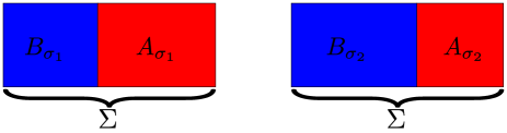
Figure 1: The families of entangling regions $A_{\sigma}$ and $B_{\sigma}$. We consider two families of entangling regions $A_{\sigma}$ (red) and $B_{\sigma}$ (blue) with $A_{\sigma_{2}}\subset A_{\sigma_{1}}$ for $\sigma_{1}<\sigma_{2}$ and $A_{\sigma}B_{\sigma}=\Sigma=const.$ In particular, this implies $B_{\sigma_{1}}\subset B_{\sigma_{2}}$.

We show that the only way how both $\Delta\left\langle{H_{0}}\right\rangle(A_{\sigma},\lambda)$ and $\Delta\left\langle{H_{0}}\right\rangle(B_{\sigma},\lambda)$ can be linear in $\tilde{\lambda}$ for all $\sigma$ in a given interval $[\xi,\eta]$ is if $\partial_{\lambda}^{2}S(A_{\sigma},\lambda)$ and $\partial_{\lambda}^{2}S(B_{\sigma},\lambda)$ are constant in $\sigma$ on $[\xi,\eta]$. The proof of this statement is a simple application of the well-known monotonicity uhlmann1977 of the RE,

$$S_{rel}(A,\lambda)\leq S_{rel}(A^{\prime},\lambda)\quad\text{if}\quad A\subseteq A^{\prime}\,,$$ (13)

and holds for any quantum system, not just for those with a holographic dual. We thus find that in the setup described above, it suffices to look at the entanglement entropies to see when higher-order contributions of $\tilde{\lambda}$ may be expected in at least one of the $\Delta\left\langle{H_{0}}\right\rangle$ (i.e. $\Delta\left\langle{H_{0}}\right\rangle(A_{\sigma},\lambda)$ or $\Delta\left\langle{H_{0}}\right\rangle(B_{\sigma},\lambda)$), namely if $\partial_{\lambda}^{2}S(A_{\sigma},\lambda)$ or $\partial_{\lambda}^{2}S(B_{\sigma},\lambda)$ is not constant in $\sigma$.

In particular if one of the $\Delta\left\langle{H_{0}}\right\rangle$, say $\Delta\left\langle{H_{0}}\right\rangle(B_{\sigma},\lambda)$, is known to be linear for all $\sigma\in[\xi,\eta]$, we learn that $\Delta\left\langle{H_{0}}\right\rangle(A_{\sigma},\lambda)$ is not. Consequently, it is not sufficient to work with entanglement entropies to determine $\Delta\left\langle{H_{0}}\right\rangle(A_{\sigma},\lambda)$ via (10), but more involved calculations are required. As a result this means that the RE is not just given by entanglement entropies.

Our result for entanglement plateaux has important consequences in particular for holographic theories. There are many well-known configurations in holography that form entanglement plateaux in the large $N$ limit. Prominent examples – which we discuss in this paper – are large intervals for the BTZ back hole Headrick:2007km ; Blanco:2013joa ; Hubeny:2013gta and two sufficiently close intervals for black strings Headrick:2010 . For these situations, very little is known about $\Delta\left\langle{H_{0}}\right\rangle$, however our result can be used to prove that non-linear $\tilde{\lambda}$ contributions play a role in the $\Delta\left\langle{H_{0}}\right\rangle$ occurring in these models. For the situation of two intervals described above, this may be used to show that the modular Hamiltonian is not an integral over the energy momentum tensor multiplied by a local scaling, as it is the case for one interval.

This paper is structured as follows. In Section 2 we consider the special case of black strings as a motivation and to introduce the basic arguments required to verify our result, which we prove in Section 3 in its full generality. We then present several situations where the result can be applied in Section 4. These include an arbitrary number of intervals for thermal states dual to black strings, a spherical shell for states dual to black branes, a sufficiently large entangling interval for states dual to BTZ black holes and primary excitations in a CFT with large central charge, defined on a circle. Furthermore, we discuss examples where the prerequisites of our result are not satisfied in Section 4.5. Finally we make some concluding remarks in Section 5.

2 A Simple Example: Black Strings

Our result for modular Hamiltonians, as described in the introduction and proved below in Section 3, may be applied to a vast variety of situations. As an illustration, we begin by a simple example that introduces the basic arguments for our result and demonstrates its usefulness. This example involves thermal CFT states in $1+1$ dimensions of inverse temperature $\beta$ with black strings as gravity duals,

$$ds_{BS}^{2}=\frac{L^{2}}{z^{2}}\Big{(}-\frac{z_{h}^{2}-z^{2}}{z_{h}^{2}}dt^{2}+\frac{z_{h}^{2}}{z_{h}^{2}-z^{2}}dz^{2}+dx^{2}\Big{)}\,,$$ (14)

where $z=z_{h}$ is the location of the black string and $L$ is the AdS radius. The asymptotic boundary, where the CFT is defined, lies at $z=0$. The energy density

$$\lambda=\frac{L}{16\pi G_{N}z_{h}^{2}}=\frac{\pi c}{6\beta^{2}}\,,$$ (15)

where $c=\frac{3L}{2G_{N}}$ is the central charge of the CFT, is chosen as the parameter for this family of states. The reference state may be chosen to correspond to any energy density $\lambda_{0}$.

We now demonstrate how the RE can be used to show that $\Delta\left\langle{H_{0}}\right\rangle$, as defined in (3), for a state living on two separated intervals is in general not linear in $\tilde{\lambda}=\lambda-\lambda_{0}$ if the two intervals are sufficiently close. The arguments that lead to this conclusion will be generalized in Section 3 below.

Consider an entangling region $A_{\sigma}$ that consists of two intervals $A^{1}_{\sigma}=[a_{1},-\sigma]$ and $A^{2}_{\sigma}=[\sigma,a_{2}]$, with $\sigma>0$ and $a_{1}$, $a_{2}$ fixed (see Figure 2). The interval $B_{\sigma}=[-\sigma,\sigma]$ between $A^{1}_{\sigma}$ and $A^{2}_{\sigma}$ is w.l.o.g. assumed to lie symmetric around the coordinate origin $x=0$.

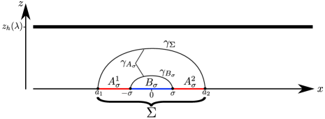
Figure 2: A constant time slice of the black string geometry (14). The asymptotic boundary of this geometry – where the CFT is defined – corresponds to the $x$-axis. The location of the black string is $z=z_{h}$ and depends on the energy density $\lambda$ via (15). If $\sigma$ is sufficiently small the RT surface $\gamma_{A_{\sigma}}$ of the entangling region $A_{\sigma}=A_{\sigma}^{1}A_{\sigma}^{2}$ (red) is the union of the RT surfaces $\gamma_{\Sigma}$ of $\Sigma=A_{\sigma}B_{\sigma}$ and $\gamma_{B_{\sigma}}$ of $B_{\sigma}$ (blue). This implies (16).

If $\sigma$ is sufficiently small, the RT surface $\gamma_{A_{\sigma}}$ of $A_{\sigma}$ is the union of $\gamma_{B_{\sigma}}$ and $\gamma_{\Sigma}$ (see Figure 2), where $\Sigma=A_{\sigma}B_{\sigma}=[a_{1},a_{2}]$ is the union of $A_{\sigma}$ and $B_{\sigma}$. Consequently, the entanglement entropy of $A_{\sigma}$ saturates the ALI Headrick:2010 , i.e.

$$S(A_{\sigma},\lambda)=S(\Sigma,\lambda)+S(B_{\sigma},\lambda)\,,$$ (16)

which is an immediate consequence of the RT formula (1). For thermal states in general CFTs defined on the real axis, the modular Hamiltonian $H_{0}(B_{\sigma})$ of $B_{\sigma}$ for the reference parameter value $\lambda_{0}$ is given by Lashkari:2014kda ; Blanco:2017xef

$$H_{0}(B_{\sigma})=\int_{-\sigma}^{\sigma}dx\,\beta_{0}\frac{\cosh(\frac{2\pi\sigma}{\beta_{0}})-\cosh(\frac{2\pi x}{\beta_{0}})}{\sinh(\frac{2\pi\sigma}{\beta_{0}})}T_{00}(x)\,,$$ (17)

where $T_{\mu\nu}$ is the energy momentum tensor of the CFT and $\beta_{0}=\beta(\lambda_{0})$. Thus, using (3), we find

$$\Delta\left\langle{H_{0}}\right\rangle(B_{\sigma},\lambda)=\beta_{0}\Big{(}2\sigma\coth\Big{(}\frac{2\pi\sigma}{\beta_{0}}\Big{)}-\frac{\beta_{0}}{\pi}\Big{)}\tilde{\lambda}=\Delta S^{\prime}(B_{\sigma},\lambda_{0})\tilde{\lambda}$$ (18)

to be linear in $\tilde{\lambda}$. Here, the ^′ refers to a derivative w.r.t. $\lambda$. The second equality is an immediate consequence of the first law of entanglement, i.e. (9), however may also be verified by a direct calculation using 2006PhRvL..96r1602R ; Calabrese:2004eu

$$S(B_{\sigma},\lambda)=\frac{c}{3}\log\Big{(}\frac{\beta}{\pi\epsilon}\sinh\Big{(}\frac{2\pi\sigma}{\beta}\Big{)}\Big{)}\ ,$$ (19)

where $\epsilon$ is a UV cutoff.

The two simple observations (16) and (18) together with the monotonicity of the RE (13) are sufficient to verify that $\Delta\left\langle{H_{0}}\right\rangle(A_{\sigma},\lambda)$ is not linear in $\tilde{\lambda}$, except for possibly one particular $\sigma$, as we now show. Let us assume that $\Delta\left\langle{H_{0}}\right\rangle(A_{\sigma},\lambda)$ is linear in $\tilde{\lambda}$ for a given $\sigma$. The first law of entanglement (9) implies

$$\Delta\left\langle{H_{0}}\right\rangle(A_{\sigma},\lambda)=\Delta S^{\prime}(A_{\sigma},\lambda_{0})\tilde{\lambda}\ .$$ (20)

Applying this result to $S_{rel}(A_{\sigma},\lambda)$ and using (16) and (18), we obtain

$$S_{rel}(A_{\sigma},\lambda)=\Delta S^{\prime}(\Sigma,\lambda_{0})\tilde{\lambda}-\Delta S(\Sigma,\lambda)+S_{rel}(B_{\sigma},\lambda)\ .$$ (21)

Using (15), (18) and (19), $S_{rel}(B_{\sigma},\lambda)$ may be brought into the form

$$S_{rel}(B_{\sigma},\lambda)=\frac{c}{3}\Big{(}\frac{1}{2}(1-b^{2})(1-a\coth(a))+\log\Big{(}b\frac{\sinh(a)}{\sinh(b\,a)}\Big{)}\Big{)}\,,$$ (22)

where $a=2\pi\sigma/\beta_{0}$ and $b=\beta_{0}/\beta$. For fixed $b$, $S_{rel}(B_{\sigma},\lambda)$ grows with $a$ (see Figure 3), which implies that $S_{rel}(B_{\sigma},\lambda)$ grows with $\sigma$ for fixed $\beta$ and $\beta_{0}$, or equivalently for fixed $\lambda$ and $\lambda_{0}$ (see (15)).

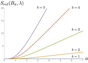
Figure 3: The behavior of $S_{rel}(B_{\sigma},\lambda)$ (22) w.r.t. $a$ for $b=1,\dots,5$, where $a=2\pi\sigma/\beta_{0}$ and $b=\beta_{0}/\beta$. We set the global prefactor $c/3=1$ and see that $S_{rel}(B_{\sigma},\lambda)$ grows with $a$ for fixed $b$. In particular, this implies that $S_{rel}(B_{\sigma},\lambda)$ grows with $B_{\sigma}$, i.e. $\sigma$, for fixed $\lambda$ and $\lambda_{0}$, which is in agreement with the monotonicity of the RE (13). For $b=1$ we find $S_{rel}(B_{\sigma},\lambda)=0$, which is to be expected from (5), since this case corresponds to $\lambda=\lambda_{0}$.

Since $S_{rel}(B_{\sigma},\lambda)$ is the only $\sigma$-dependent term on the RHS of (21), $S_{rel}(A_{\sigma},\lambda)$ grows with $\sigma$ as well. Now assume there were two values $\xi$, $\eta$ for $\sigma$, where we set w.lo.g. $\xi<\eta$, for which $\Delta\left\langle{H_{0}}\right\rangle(A_{\sigma},\lambda)$ is linear in $\tilde{\lambda}$. From the above discussion we conclude

$$S_{rel}(A_{\xi},\lambda)<S_{rel}(A_{\eta},\lambda)\,.$$ (23)

However, the monotonicity of the RE (13) implies that $S_{rel}(A_{\eta},\lambda)$ must be smaller than $S_{rel}(A_{\xi},\lambda)$, since $A_{\eta}\subset A_{\xi}$. So by assuming $\Delta\left\langle{H_{0}}\right\rangle(A_{\sigma},\lambda)$ to be linear in $\tilde{\lambda}$ for more than one value of $\sigma$, we encounter a contradiction. Consequently, $\Delta\left\langle{H_{0}}\right\rangle(A_{\sigma},\lambda)$ may be linear in $\tilde{\lambda}$ for at most one particular $\sigma$.

This simple example shows that even though the modular Hamiltonian for two disconnected intervals is unknown, general properties of the RE imply that the modular Hamiltonian necessarily involves contributions of higher order in $\tilde{\lambda}$. An immediate consequence of this observation is that the modular Hamiltonian for two intervals, unlike for one interval (17), can not be of the simple form

$$\int_{A_{\sigma}}dxf^{\mu\nu}(x)T_{\mu\nu}(x)\,,$$ (24)

where $f^{\mu\nu}$ is a local weight function, since this would lead to a $\Delta\left\langle{H_{0}}\right\rangle(A_{\sigma},\lambda)$ that is linear in $\tilde{\lambda}$.

Note that since $S_{rel}(B_{\sigma},\lambda)$ is known, we are not required to consider $\partial^{2}_{\lambda}S$, i.e. the quantity discussed below (13) in the introduction. We were able to deduce the non-linearity of $\Delta\left\langle{H_{0}}\right\rangle(A_{\sigma},\lambda)$ directly from $S_{rel}(B_{\sigma},\lambda)$ (see (21)). In the more general cases discussed in Section 3, where $S_{rel}(B_{\sigma},\lambda)$ is not known, this is no longer possible.

3 Generic Entanglement Plateaux

We now generalize the approach introduced in Section 2 and show how the RE determines whether non-linear contributions to $\Delta\left\langle{H_{0}}\right\rangle$ in $\tilde{\lambda}$ are to be expected. Note that we do not require $\lambda$ to be the energy density, it is just the variable that parametrizes the family of states $\rho_{\lambda}$ we consider.

The discussion in Section 2 required the saturation of the ALI (11), which allowed us to show that if $\Delta\left\langle{H_{0}}\right\rangle$ were linear in $\tilde{\lambda}$, the RE would increase when the size of the considered entangling region (i.e. two intervals) decreases. However, due to the monotonicity of the RE (13) this is not possible.

By looking at (21), we see that this contradiction does not require the explicit expressions for the (relative) entropies: If $S_{rel}(B_{\sigma},\lambda)$ grows with $B_{\sigma}$ for fixed $\Sigma$, $S_{rel}(A_{\sigma},\lambda)$ grows as well. However, this is not compatible with the monotonicity of $S_{rel}$, since $A_{\sigma}=\Sigma\backslash B_{\sigma}$ decreases if $B_{\sigma}$ increases. This fact allows us to generalize the arguments of Section 2 to generic entanglement plateaux, i.e. systems that saturate the ALI.

3.1 Result for Generic Entanglement Plateaux

In the general case, the prerequisites for our main statement are as follows. We consider a one-parameter family of states $\rho_{\lambda}$. Let $\Sigma$ be an entangling region and $A_{\sigma}\subseteq\Sigma$ a one-parameter family of decreasing subregions of $\Sigma$, i.e. $A_{\sigma_{2}}\subset A_{\sigma_{1}}$ for $\sigma_{1}<\sigma_{2}$, where the parameter $\sigma$ is assumed to be continuous. Furthermore, let $B_{\sigma}=\Sigma\backslash A_{\sigma}$ be the complement of $A_{\sigma}$ w.r.t. $\Sigma$ (see Figure 1). Moreover, the ALI (11) is assumed to be saturated for $A_{\sigma}$ and $B_{\sigma}$, i.e.

$$|S(A_{\sigma},\lambda)-S(B_{\sigma},\lambda)|=S(\Sigma,\lambda)\quad\forall\sigma,\lambda\,.$$ (25)

Furthermore, $S(A_{\sigma},\lambda)$, $S(B_{\sigma},\lambda)$ and $S(\Sigma,\lambda)$ are considered to be differentiable in $\lambda$ for all $\sigma$.

Subject to these prerequisites, we now state our main result. If both $\Delta\left\langle{H_{0}}\right\rangle(A_{\sigma},\lambda)$ and $\Delta\left\langle{H_{0}}\right\rangle(B_{\sigma},\lambda)$ are linear in $\tilde{\lambda}=\lambda-\lambda_{0}$ for all $\sigma$ in a given interval $[\xi,\eta]$, then $\partial_{\lambda}^{2}S(A_{\sigma},\lambda)$ and $\partial_{\lambda}^{2}S(B_{\sigma},\lambda)$ are constant in $\sigma$ on $[\xi,\eta]$ for all $\lambda$.
We prove this statement as follows. As we discuss in the appendix, w.l.o.g. we may restrict our arguments to the case $S(A_{\sigma},\lambda)\geq S(B_{\sigma},\lambda)$. Assume that for all $\sigma\in[\xi,\eta]$, both $\Delta\left\langle{H_{0}}\right\rangle(A_{\sigma},\lambda)$ and $\Delta\left\langle{H_{0}}\right\rangle(B_{\sigma},\lambda)$ are linear in $\tilde{\lambda}$. Then, as explained in the introduction (see (10)), we find

$$\Delta\left\langle{H_{0}}\right\rangle(A_{\sigma},\lambda)=\Delta S^{\prime}(A_{\sigma},\lambda_{0})\tilde{\lambda}\quad\mbox{and}\quad\Delta\left\langle{H_{0}}\right\rangle(B_{\sigma},\lambda)=\Delta S^{\prime}(B_{\sigma},\lambda_{0})\tilde{\lambda}\,,$$ (26)

where ^′ again refers to a derivative w.r.t. $\lambda$. This implies together with (5) and (25)

$$S_{rel}(A_{\sigma},\lambda)=\Delta S^{\prime}(\Sigma,\lambda_{0})\tilde{\lambda}-\Delta S(\Sigma,\lambda)+S_{rel}(B_{\sigma},\lambda)\,.$$ (27)

Due to the monotonicity (13) of $S_{rel}$ we find

$$S_{rel}(B_{\xi},\lambda)\leq S_{rel}(B_{\eta},\lambda)\,,$$ (28)

since $B_{\xi}\subset B_{\eta}$. Using (27), this implies

$$S_{rel}(A_{\xi},\lambda)\leq S_{rel}(A_{\eta},\lambda)\,.$$ (29)

By construction we have $A_{\eta}\subset A_{\xi}$. So the only way how (29) may be compatible with the monotonicity of $S_{rel}$ is if $S_{rel}(A_{\sigma},\lambda)$ is constant in $\sigma$ for $\sigma\in[\xi,\eta]$. Thus by using (5) and (26), we find

$$-\partial^{2}_{\lambda}S_{rel}(A_{\sigma},\lambda)=-\partial^{2}_{\lambda}(\Delta S^{\prime}(A_{\sigma},\lambda_{0})(\lambda-\lambda_{0})-\Delta S(A_{\sigma},\lambda))=\partial^{2}_{\lambda}S(A_{\sigma},\lambda)$$ (30)

to be constant in $\sigma$ on $[\xi,\eta]$.

Due to (27) the fact that $S_{rel}(A_{\sigma},\lambda)$ is constant in $\sigma$ for $\sigma\in[\xi,\eta]$ implies that $S_{rel}(B_{\sigma},\lambda)$ is as well. In an analogous way as for $A_{\sigma}$, we find $\partial_{\lambda}^{2}S(B_{\sigma},\lambda)$ to be constant in $\sigma$ on $[\xi,\eta]$. This completes the proof of the general result stated at the beginning of this section.

3.2 Discussion for Generic Entanglement Plateaux

In Section 3.1 we presented our result for a generic situation where the ALI is saturated. Some comments are in order.

First we note that even though we presented an example from holography in Section 2 as a motivation, we did not require holography at any point during the proof. Therefore our result is true for any quantum system.

Furthermore, we required $\sigma$, i.e. the parameter of the family of entangling regions $A_{\sigma}$, to be continuous, as can be read off the discussion in the appendix. However, if we in addition assume the sign of $S(A_{\sigma},\lambda)-S(B_{\sigma},\lambda)$ to be constant in $\sigma$, we can apply the result to discrete systems, such as spin-chains, as well. The proof works analogously as in the continuous case discussed in Section 3.1.

In Section 3.1 we showed that $\partial_{\lambda}^{2}S(A_{\sigma},\lambda)$ and $\partial_{\lambda}^{2}S(B_{\sigma},\lambda)$ beeing constant in $\sigma$ on an interval $[\xi,\eta]$ is a necessary condition for both $\Delta\left\langle{H_{0}}\right\rangle(A_{\sigma},\lambda)$ and $\Delta\left\langle{H_{0}}\right\rangle(B_{\sigma},\lambda)$ to be linear in $\tilde{\lambda}$ for all $\sigma\in[\xi,\eta]$. However, this condition is not sufficient, as we now demonstrate by presenting an example where $\partial_{\lambda}^{2}S(A_{\sigma},\lambda)$ and $\partial_{\lambda}^{2}S(B_{\sigma},\lambda)$ are constant in $\sigma$ but both $\Delta\left\langle{H_{0}}\right\rangle(A_{\sigma},\lambda)$ and $\Delta\left\langle{H_{0}}\right\rangle(B_{\sigma},\lambda)$ are not linear in $\tilde{\lambda}$.

We consider a free massless boson CFT in two dimensions defined on a circle with radius $\ell_{CFT}$. The family of states is chosen to consist of exited states of the form

$$|{\lambda}\rangle=e^{i\sqrt{2\lambda}\Phi}|{0}\rangle\,,$$ (31)

where $\Phi$ is the boson field and $|{0}\rangle$ is the vacuum state. We use their conformal dimension $(\lambda,0)$ to parametrize these states. For the sake of this paper we assume the conformal dimension $\lambda$ to be a continuous parameter. We define $A_{\sigma}$ to be an interval of angular size $2(\pi-\sigma)$ and $B_{\sigma}=A_{\sigma}^{c}$ to be the complementary interval of angular size $2\sigma$. Consequently, $\Sigma=A_{\sigma}B_{\sigma}$ is the entire circle and the fact that $|{\lambda}\rangle$ is pure implies $S(\Sigma,\lambda)=0$ and $S(A_{\sigma},\lambda)=S(B_{\sigma},\lambda)$, and therefore the saturation of the ALI (11). The reference state $|{\lambda_{0}}\rangle$ can be chosen arbitrarily. This setup was discussed in Lashkari:2015dia , where the RE was found to be

$$S_{rel}(A_{\sigma},\lambda) =(1+(\pi-\sigma)\cot(\sigma))\Big{(}\sqrt{2\lambda}-\sqrt{2\lambda_{0}}\Big{)}^{2}\,,$$ (32)

$$S_{rel}(B_{\sigma},\lambda) =(1-\sigma\cot(\sigma))\Big{(}\sqrt{2\lambda}-\sqrt{2\lambda_{0}}\Big{)}^{2}\,.$$ (33)

The author of Lashkari:2015dia states that the entanglement entropies of $A_{\sigma}$ and $B_{\sigma}$ are constant in $\lambda$. Therefore, by applying (5) to (32) and (33) we find

$$\Delta\left\langle{H_{0}}\right\rangle(A_{\sigma},\lambda) =(1+(\pi-\sigma)\cot(\sigma))\Big{(}\sqrt{2\lambda}-\sqrt{2\lambda_{0}}\Big{)}^{2}\,,$$ (34)

$$\Delta\left\langle{H_{0}}\right\rangle(B_{\sigma},\lambda) =(1-\sigma\cot(\sigma))\Big{(}\sqrt{2\lambda}-\sqrt{2\lambda_{0}}\Big{)}^{2}\,.$$ (35)

Obviously, both $\Delta\left\langle{H_{0}}\right\rangle(A_{\sigma},\lambda)$ and $\Delta\left\langle{H_{0}}\right\rangle(B_{\sigma},\lambda)$ are not linear in $\tilde{\lambda}=\lambda-\lambda_{0}$. However, since the entanglement entropy is constant in $\lambda$, we find $\partial_{\lambda}^{2}S=0$ for $A_{\sigma}$ and $B_{\sigma}$, and therefore that $\partial_{\lambda}^{2}S$ is constant in $\sigma$ for $A_{\sigma}$ and $B_{\sigma}$. Thus we see that $\partial_{\lambda}^{2}S$ being constant in $\sigma$ does not imply that both $\Delta\left\langle{H_{0}}\right\rangle(A_{\sigma},\lambda)$ and $\Delta\left\langle{H_{0}}\right\rangle(B_{\sigma},\lambda)$ are linear in $\tilde{\lambda}$. Therefore it is a necessary but not a sufficient condition.

The proof of our result presented in Section 3.1 strongly relies on the first law of entanglement (8). We need to emphasize that the first law of entanglement only applies if the reference state corresponds to a parameter value $\lambda_{0}$ that is not a boundary point of the set of allowed parameter values $\lambda$. The fact that the first law of entanglement holds is a consequence of the non-negativity of $S_{rel}(A,\lambda)$ and $S_{rel}(A,\lambda_{0})=0$. These two properties imply that $S_{rel}$ is minimal at $\lambda=\lambda_{0}$ and therefore we find

$$\partial_{\lambda}S_{rel}(A,\lambda)|_{\lambda=\lambda_{0}}=0\,.$$ (36)

Using (5) it is easy to see that (36) is equivalent to the first law of entanglement. However, if $\lambda_{0}$ is a boundary point of the set of allowed $\lambda$, i.e. if it is not possible to choose $\lambda<\lambda_{0}$ for instance, the minimality of $S_{rel}(A,\lambda_{0})$ does not necessarily imply $\partial_{\lambda}S_{rel}(A,\lambda)|_{\lambda=\lambda_{0}}$ to vanish.

The free massless boson CFT we discuss above is an example for such a situation. Here the parameter $\lambda$ is the conformal dimension of the considered states and is therefore non-negative. By choosing the reference state to be the vacuum, i.e. $\lambda_{0}=0$, (32) gives

$$S_{rel}(A_{\sigma},\lambda)=2(1+(\pi-\sigma)\cot(\sigma))\tilde{\lambda}\,,$$ (37)

and therefore $\partial_{\lambda}S_{rel}(A_{\sigma},\lambda)|_{\lambda=\lambda_{0}}\neq 0$. Consequently, the first law of entanglement does not hold for this example. Even though it has the expected properties according to our prediction, i.e. both $\Delta\left\langle{H_{0}}\right\rangle(A_{\sigma},\lambda)$ and $\Delta\left\langle{H_{0}}\right\rangle(B_{\sigma},\lambda)$ are linear in $\tilde{\lambda}$ and $\partial_{\lambda}^{2}S(A_{\sigma},\lambda)$ and $\partial_{\lambda}^{2}S(B_{\sigma},\lambda)$ are constant in $\sigma$ (see (34), (35) for $\lambda_{0}=0$), the prerequisites of our result are not satisfied if the first law of entanglement does not hold.

We only considered one-parameter families of states in Section 3.1. However, our result can be straightforwardly generalized to an $n$-parameter family of states $\rho_{\Lambda}$ with $\Lambda=(\lambda^{1},...,\lambda^{n})$. The reference state corresponds to $\Lambda=\Lambda_{0}=(\lambda^{1}_{0},...,\lambda^{n}_{0})$. In an analogous way as for the one-parameter case we can show that the only way how both $\Delta\left\langle{H_{0}}\right\rangle(A_{\sigma},\Lambda)$ and $\Delta\left\langle{H_{0}}\right\rangle(B_{\sigma},\Lambda)$ can be linear in $\Lambda-\Lambda_{0}$, i.e. of the form

$$\begin{split}&\Delta\left\langle{H_{0}}\right\rangle(A_{\sigma},\Lambda)=\partial_{i}\Delta S(A_{\sigma},\Lambda)|_{\Lambda=\Lambda_{0}}(\lambda^{i}-\lambda_{0}^{i})\,\\ &\Delta\left\langle{H_{0}}\right\rangle(B_{\sigma},\Lambda)=\partial_{i}\Delta S(B_{\sigma},\Lambda)|_{\Lambda=\Lambda_{0}}(\lambda^{i}-\lambda_{0}^{i})\,,\end{split}$$ (38)

where $\partial_{i}=\partial/\partial\lambda^{i}$, for all $\sigma\in[\xi,\eta]$ is if $\partial_{i}\partial_{j}S(A_{\sigma},\Lambda)$ and $\partial_{i}\partial_{j}S(B_{\sigma},\Lambda)$ are constant in $\sigma$ on $[\xi,\eta]$.

3.3 Alternative Formulation

For the examples we discuss in Section 4, it is more convenient to use the following alternative formulation of our result:

Consider the assumptions necessary for the result to be satisfied (see Section 3.1). If $\partial_{\lambda}^{2}S(A_{\sigma},\lambda)$ or $\partial_{\lambda}^{2}S(B_{\sigma},\lambda)$ is not constant in $\sigma$ on any interval $[\xi,\eta]$, then there are only single values of $\sigma$ where both $\Delta\left\langle{H_{0}}\right\rangle(A_{\sigma},\lambda)$ and $\Delta\left\langle{H_{0}}\right\rangle(B_{\sigma},\lambda)$ are linear in $\tilde{\lambda}$, i.e. there is no interval $[\xi,\eta]$ where both $\Delta\left\langle{H_{0}}\right\rangle(A_{\sigma},\lambda)$ and $\Delta\left\langle{H_{0}}\right\rangle(B_{\sigma},\lambda)$ are linear in $\tilde{\lambda}$ for all $\sigma\in[\xi,\eta]$.

In the original formulation, the linearity of $\Delta\left\langle{H_{0}}\right\rangle(A_{\sigma},\lambda)$ and $\Delta\left\langle{H_{0}}\right\rangle(B_{\sigma},\lambda)$ in $\tilde{\lambda}$ implies that the second derivative of the entanglement entropies of $A_{\sigma}$ and $B_{\sigma}$ are constant in $\sigma$. In the alternative formulation however, non-constancy in $\sigma$ of the second derivative of one of the entanglement entropies implies that in general $\Delta\left\langle{H_{0}}\right\rangle$ is non-linear in $\tilde{\lambda}$ for $A_{\sigma}$, $B_{\sigma}$ or both. In the examples of Section 4, there are non-constant second derivatives of the entanglement entropies, and therefore the alternative formulation is more appropriate.

In the alternative formulation, the number of values for $\sigma$ where both $\Delta\left\langle{H_{0}}\right\rangle(A_{\sigma},\lambda)$ and $\Delta\left\langle{H_{0}}\right\rangle(B_{\sigma},\lambda)$ are linear in $\tilde{\lambda}$ is undetermined. However, in Section 2, where we considered $A_{\sigma}$ to be the union of two intervals, we were able to show a stronger statement. We found that there is at most one such value for $\sigma$ and moreover, that $\Delta\left\langle{H_{0}}\right\rangle(A_{\sigma},\lambda)$ is linear in $\tilde{\lambda}$ only for that value of $\sigma$. The arguments of Section 2 that lead to this conclusion can be generalized to the case of generic entanglement plateaux if

$$D_{rel}(B_{\sigma},\lambda)=\Delta S^{\prime}(B_{\sigma},\lambda_{0})\tilde{\lambda}-\Delta S(B_{\sigma},\lambda)$$ (39)

grows strictly monotonically with $\sigma$. In particular, if $\Delta\left\langle{H_{0}}\right\rangle(B_{\sigma},\lambda)$ is known to be linear in $\tilde{\lambda}$, $D_{rel}(B_{\sigma},\lambda)$ is the RE of $B_{\sigma}$, which is the case for the setup discussed in Section 2, for instance.

Just as in Section 3.1, we assume w.l.o.g. $S(A_{\sigma},\lambda)\geq S(B_{\sigma},\lambda)$. Under the assumption that there are two values $\xi$, $\eta$ for $\sigma$ where $\Delta\left\langle{H_{0}}\right\rangle(A_{\sigma},\lambda)$ is linear in $\tilde{\lambda}$, we find, analogous to the derivation of (27),

$$S_{rel}(A_{\xi,\eta},\lambda)=\Delta S^{\prime}(\Sigma,\lambda_{0})\tilde{\lambda}-\Delta S(\Sigma,\lambda)+D_{rel}(B_{\xi,\eta},\lambda)\,.$$ (40)

Since $D_{rel}(B_{\sigma},\lambda)$ is assumed to grow strictly monotonically with $\sigma$, this implies for $\xi<\eta$

$$S_{rel}(A_{\xi},\lambda)<S_{rel}(A_{\eta},\lambda)\,,$$ (41)

which is not possible due to the monotonicity of $S_{rel}$ (13), since $A_{\eta}\subset A_{\xi}$. Consequently, there can only be one value of $\sigma$ where $\Delta\left\langle{H_{0}}\right\rangle(A_{\sigma},\lambda)$ is linear in $\tilde{\lambda}$.

4 Applications

We now apply the general result of Section 3.1 to holographic states dual to black strings, black branes and BTZ black holes. Moreover, we apply the result to pure states, which we first discuss in full generality and then consider primary excitations of a CFT with large central charge as an example. In all these configurations entanglement plateaux can be constructed, i.e. situations where the ALI is saturated (25), which is the only requirement for our result.

4.1 Black Strings Revisited

First we consider once more, as in Section 2, the situation of two sufficiently close intervals for CFTs dual to black strings (14). The parameter $\lambda$ is chosen to be the energy density (15). We can confirm the conclusion we made in Section 2 by applying the result of Section 3.1:

Using (19) is easy to see that $\partial_{\lambda}^{2}S(B_{\sigma},\lambda)$ is not constant in $\sigma$ on any interval. So the result of Section 3.1 tells us that there is no interval $[\xi,\eta]$ where both $\Delta\left\langle{H_{0}}\right\rangle(A_{\sigma},\lambda)$ and $\Delta\left\langle{H_{0}}\right\rangle(B_{\sigma},\lambda)$ are linear in $\tilde{\lambda}$ for all $\sigma\in[\xi,\eta]$. We know that $\Delta\left\langle{H_{0}}\right\rangle(B_{\sigma},\lambda)$ is linear in $\tilde{\lambda}$ for all $\sigma$ (see (18)), and therefore conclude that $\Delta\left\langle{H_{0}}\right\rangle(A_{\sigma},\lambda)$ is not, except possibly for single values of $\sigma$.

From the discussion in Section 3.3 we are even able to conclude that there is only one such $\sigma$. This is due to the fact that $D_{rel}(B_{\sigma},\lambda)$ (39), which is equal to $S_{rel}(B_{\sigma},\lambda)$ here, grows strictly monotonically with $\sigma$, as pointed out in Section 2. This special value of $\sigma$ corresponds to the degenerate situation where $B_{\sigma}$ vanishes and $A_{\sigma}$ becomes a single interval, i.e. $\sigma=0$.

The discussion of two intervals can be straightforwardly generalized to the situation of $A_{\sigma}$ being the union of an arbitrary number of intervals. $B_{\sigma}$ is chosen to be an interval between two neighboring intervals that belong to $A_{\sigma}$. If the ALI is saturated, which corresponds to a situation such as the one depicted in Figure 4, we see in analogy to the two-interval case, that $\Delta\left\langle{H_{0}}\right\rangle(A_{\sigma},\lambda)$ is in general not linear in $\tilde{\lambda}$.

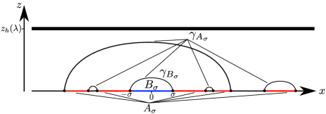
Figure 4: A constant time slice of the black string geometry (14) revisited. The asymptotic boundary of this geometry – where the CFT is defined – corresponds to the $x$-axis. The location of the black string is $z=z_{h}$ and depends on the energy density $\lambda$ via (15). It is possible to choose a union of intervals $A_{\sigma}$ (red) and an interval $B_{\sigma}$ (blue) that lies between two intervals that belong to $A_{\sigma}$ in such a way that $A_{\sigma}$ and $B_{\sigma}$ saturate the ALI, i.e. (25).

4.2 Thermal States Dual to Black Branes

Consider thermal CFT states on $d$-dimensional Minkowski space that are dual to black branes,

$$ds^{2}_{BB}=\frac{L^{2}}{z^{2}}\Big{(}-\frac{z_{h}^{d}-z^{d}}{z_{h}^{d}}dt^{2}+\frac{z_{h}^{d}}{z_{h}^{d}-z^{d}}dz^{2}+d\vec{x}_{d-1}^{2}\Big{)}\ ,$$ (42)

where the black brane is located at $z=z_{h}$. Just as for black strings (see Section 2) the asymptotic boundary, where the CFT is defined, corresponds to $z=0$. We choose $\Sigma$ to be a ball with radius $R$ and $B_{\sigma}$ another ball with radius $\sigma<R$ with the same center as $\Sigma$. Consequently, $A_{\sigma}=\Sigma\backslash B_{\sigma}$ is a spherical shell with inner radius $\sigma$ and outer radius $R$. We choose $\lambda$ to be the energy density of the considered thermal states,

$$\lambda=\frac{(d-1)L^{d-1}}{16\pi G_{N}z_{h}^{d}}\,.$$ (43)

The reference state is chosen to be the ground state, i.e. $\lambda_{0}=0$. If we only consider sufficiently small radii $\sigma$, such that the RT surface of $A_{\sigma}$ is given by the union of the RT surfaces of $\Sigma$ and $B_{\sigma}$ for all $\sigma$, we find the ALI to be saturated for this setup (see Figure 2 for $d=2$). Furthermore, we know $\Delta\left\langle{H_{0}}\right\rangle(B_{\sigma},\lambda)$ to be linear in $\tilde{\lambda}$ for all $\sigma$ Blanco:2013joa ,

$$\Delta\left\langle{H_{0}}\right\rangle(B_{\sigma},\lambda)=\frac{2\pi\Omega_{d-2}}{d^{2}-1}\sigma^{d}\tilde{\lambda}\,,$$ (44)

where $\Omega_{d-2}=\frac{2\pi^{(d-1)/2}}{\Gamma((d-1)/2)}$. Moreover, $S(B_{\sigma},\lambda)$ is given, via the RT formula (1), by Blanco:2013joa

$$S(B_{\sigma},\lambda)=\frac{L^{d-1}\Omega_{d-2}}{4G_{N}}\int_{0}^{\sigma}d\rho\frac{\rho^{d-2}}{z(\rho)^{d-1}}\sqrt{1+\frac{(\partial_{\rho}z(\rho))^{2}z_{h}^{d}}{z_{h}^{d}-z(\rho)^{d}}}\,,$$ (45)

where $z(\rho)$ has to be chosen in such a way, that the integral on the RHS of (45) is minimized. To our knowledge there is no analytic, integral free expression for $S(B_{\sigma},\lambda)$ for generic $d$. However, in Blanco:2013joa an expansion of $\Delta S(B_{\sigma},\lambda)$ in $\alpha\,\sigma^{d}\lambda$ is presented, with $\alpha=\frac{16\pi G_{N}}{dL^{d-1}}$,

$$\Delta S(B_{\sigma},\lambda)=\frac{\Omega_{d-2}L^{d-1}}{4G_{N}}\Big{(}\frac{d\,\alpha\,\sigma^{d}\lambda}{2(d^{2}-1)}-\frac{d^{3}\sqrt{\pi}\,\Gamma(d-1)\alpha^{2}\sigma^{2d}\lambda^{2}}{2^{d+4}(d+1)\Gamma\Big{(}d+\frac{3}{2}\Big{)}}+\mathcal{O}((\alpha\sigma^{d}\lambda)^{3})\Big{)}\,.$$ (46)

Due to $\partial_{\lambda}^{2}\Delta S(B_{\sigma},\lambda)=\partial_{\lambda}^{2}S(B_{\sigma},\lambda)$, we see that $\partial_{\lambda}^{2}S(B_{\sigma},\lambda)$ is not constant in $\sigma$ on any interval. Since $\Delta\left\langle{H_{0}}\right\rangle(B_{\sigma},\lambda)$ is linear in $\tilde{\lambda}$ (44) for all $\sigma$, the result of Section 3.1 now tells us that $\Delta\left\langle{H_{0}}\right\rangle(A_{\sigma},\lambda)$ may only be linear in $\tilde{\lambda}$ for single values of $\sigma$.

Just as for the black string, we can even show that there is only one such $\sigma$. From (44) and (46) we conclude that $S_{rel}(B_{\sigma},\lambda)$ (5) is not constant in $\sigma$ on any interval. The monotonicity (13) of the RE then implies that $S_{rel}(B_{\sigma},\lambda)$ grows strictly monotonically with $\sigma$. Since $\Delta\left\langle{H_{0}}\right\rangle(B_{\sigma},\lambda)$ is linear in $\tilde{\lambda}$ we find $D_{rel}(B_{\sigma},\lambda)=S_{rel}(B_{\sigma},\lambda)$ (39) and therefore conclude that $D_{rel}(B_{\sigma},\lambda)$ grows strictly monotonically with $\sigma$. The discussion in Section 3.3 now implies that there is at most one value of $\sigma$ where $\Delta\left\langle{H_{0}}\right\rangle(A_{\sigma},\lambda)$ is linear in $\tilde{\lambda}$. This special $\sigma$ can be found to be the degenerate case $\sigma=0$, i.e. when $B_{\sigma}$ vanishes.

4.3 BTZ Black Hole

As a further application of the result of Section 3.1 to holography we consider thermal states dual to BTZ black hole geometries,

$$ds_{BTZ}^{2}=-\frac{r^{2}-r_{h}^{2}}{L^{2}}dt^{2}+\frac{L^{2}}{r^{2}-r_{h}^{2}}dr^{2}+r^{2}d\phi^{2}\,.$$ (47)

The horizon radius $r_{h}$ is given – in terms of the CFT temperature $T$ and the radius $\ell_{CFT}$ of the circle on which the CFT is defined – by

$$r_{h}=\sqrt{8G_{N}M}L=2\pi L\ell_{CFT}T\,,$$ (48)

where $M$ is the mass of the BTZ black hole.

The asymptotic boundary, where the CFT is defined, corresponds to $r\rightarrow\infty$. For an interval $A_{\sigma}$ of sufficiently large angular size $2(\pi-\sigma)$, the RT surface consists of two disconnected parts: the horizon and the RT surface of $A^{c}_{\sigma}=B_{\sigma}$, as depicted in Figure 5.

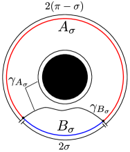
Figure 5: A constant time slice of the BTZ black hole geometry (47). The CFT is defined on the asymptotic boundary at $r\rightarrow\infty$. For a sufficiently large entangling region $A_{\sigma}$ (red) the RT surface $\gamma_{A_{\sigma}}$ is the union of the RT surface $\gamma_{B_{\sigma}}$ of its complement $B_{\sigma}$ (blue) and the black hole horizon. This implies (25).

The entanglement entropy is then given by Headrick:2007km ; Blanco:2013joa

$$S(A_{\sigma})=\frac{c}{3}2\pi^{2}T\ell_{CFT}+\frac{c}{3}\log\Big{(}\frac{1}{\pi T\epsilon}\sinh(2\pi\ell_{CFT}T\sigma)\Big{)}\,,$$ (49)

where $\epsilon$ is a UV cutoff. The first term is the thermal entropy of the state and corresponds to the black hole horizon, while the second term is the entanglement entropy of $B_{\sigma}$. We see once more that the states on $A_{\sigma}$ and $B_{\sigma}$ saturate the ALI. As parameter $\lambda$ for this family of states we choose the square of the temperature,

$$\lambda=T^{2}\,,$$ (50)

which corresponds to the mass $M$ of the black hole,

$$LM=\frac{\pi^{2}\ell_{CFT}^{2}c}{3}\lambda\,.$$ (51)

The reference state can be chosen to correspond to any $\lambda=\lambda_{0}=T_{0}^{2}$. Using (49) it is straight forward to see that $\partial_{\lambda}^{2}S(A_{\sigma},\lambda)$ is not constant in $\sigma$ on any interval. So, even though the explicit forms of $\Delta\left\langle{H_{0}}\right\rangle(A_{\sigma},\lambda)$ and $\Delta\left\langle{H_{0}}\right\rangle(B_{\sigma},\lambda)$ (3) are not known, we can use the result of Section 3.1 to conclude that in general at least one of $\Delta\left\langle{H_{0}}\right\rangle(A_{\sigma},\lambda)$ or $\Delta\left\langle{H_{0}}\right\rangle(B_{\sigma},\lambda)$ is not linear in $\tilde{\lambda}=T^{2}-T_{0}^{2}$.

Note that the result of Section 3.1 cannot be used to determine whether $\Delta\left\langle{H_{0}}\right\rangle(A_{\sigma},\lambda)$, $\Delta\left\langle{H_{0}}\right\rangle(B_{\sigma},\lambda)$ or both are non-linear in $\tilde{\lambda}$. However, the discussion in Section 3.3 actually allows us to show that $\Delta\left\langle{H_{0}}\right\rangle(A_{\sigma},\lambda)$ is not linear in $\tilde{\lambda}$ for more than one particular $\sigma$: By applying $S(B_{\sigma},\lambda)$, i.e. the second term in (49), to (39) we find

$$D_{rel}(B_{\sigma},\lambda)=\frac{c}{3}\Big{(}\frac{1}{2}\big{(}1-\tilde{a}\coth(\tilde{a})\big{)}(1-\tilde{b}^{2})+\log\Big{(}\tilde{b}\frac{\sinh(\tilde{a})}{\sinh(\tilde{b}\,\tilde{a})}\Big{)}\Big{)}\,,$$ (52)

where $\tilde{a}=2\pi\ell_{CFT}\sqrt{\lambda_{0}}\sigma$ and $\tilde{b}=\sqrt{\lambda}/\sqrt{\lambda_{0}}$. The structure of the $\sigma$ dependence of $D_{rel}(B_{\sigma},\lambda)$ is identical to the structure of the $\sigma$ dependence of $S_{rel}(B_{\sigma},\lambda)$ that was derived in Section 2 for two intervals (see (21) and (22)). So in an analogous way to the discussion in Section 2, we find that $D_{rel}(B_{\sigma},\lambda)$ grows strictly monotonically with $\sigma$. Consequently, $\Delta\left\langle{H_{0}}\right\rangle(A_{\sigma},\lambda)$ is not linear in $\tilde{\lambda}$ except for possibly one particular $\sigma$.

4.4 Pure States: Primary Excitations in CFTs with Large Central Charge

It is also possible to apply the result of Section 3.1 to a one-parameter family of pure states. Consider $\rho_{\lambda}$ to be such a family and $\Sigma$ to be the entire constant time slice, i.e. $B_{\sigma}=A_{\sigma}^{c}$. Since $S(\Sigma,\lambda)=0$ and $S(A_{\sigma},\lambda)=S(B_{\sigma},\lambda)$, the ALI is saturated for this setup. The result of Section 3.1 now tells us that if $\partial_{\lambda}^{2}S(A_{\sigma},\lambda)$ is not constant in $\sigma$ on any interval $[\xi,\eta]$, it is not possible for $\Delta\left\langle{H_{0}}\right\rangle(A_{\sigma},\lambda)$ and $\Delta\left\langle{H_{0}}\right\rangle(B_{\sigma},\lambda)$ to be linear in $\tilde{\lambda}$ for the same $\sigma$, except for single values of $\sigma$.

As an example for such a family of pure states we consider spinless primary excitations $|{\lambda}\rangle$ in a CFT with large central charge $c$ defined on a circle with radius $\ell_{CFT}$. We use the conformal dimension

$$(h_{\lambda},\bar{h}_{\lambda})=\Big{(}\frac{c\lambda}{24},\frac{c\lambda}{24}\Big{)}$$ (53)

to parametrize these states and assume $|{\lambda}\rangle$ to correspond to a heavy operator, i.e. $\Delta_{\lambda}=h_{\lambda}+\bar{h}_{\lambda}=\mathcal{O}(c)$. Moreover, we restrict our analysis to the case $\lambda<1$ and assume the spectrum of light operators, i.e. operators with $\Delta=h+\bar{h}\ll c$, to be sparse. The entangling regions $\Sigma$ and $B_{\sigma}$ are chosen to be the entire circle and an interval with angular size $2\sigma<\pi$, respectively. Consequently, $A_{\sigma}=B_{\sigma}^{c}$ is an interval with angular size $2(\pi-\sigma)>\pi$. The reference state corresponds to an arbitrary value $\lambda_{0}$ of the parameter $\lambda$.

The entanglement entropy of $B_{\sigma}$ for this setup was computed in Asplund:2014coa ,

$$S(B_{\sigma},\lambda)=\frac{c}{3}\log\Big{(}\frac{2\ell_{CFT}}{\sqrt{1-\lambda}\,\epsilon}\sin\big{(}\sqrt{1-\lambda}\,\sigma\big{)}\Big{)}=S(A_{\sigma},\lambda)\,,$$ (54)

where $\epsilon$ is a UV cutoff. The second equality in (54) is a consequence of the fact that $|{\lambda}\rangle$ is pure and ensures that the ALI is saturated. It is easy to see that $\partial_{\lambda}^{2}S(B_{\sigma},\lambda)$ is not constant in $\sigma$ on any interval. Therefore the result of Section 3.1 implies that there are only single values of $\sigma$ where both $\Delta\left\langle{H_{0}}\right\rangle(A_{\sigma},\lambda)$ and $\Delta\left\langle{H_{0}}\right\rangle(B_{\sigma},\lambda)$ are linear in $\tilde{\lambda}=\lambda-\lambda_{0}$.

Analogously to the discussion regarding BTZ black holes in Section 4.3, we can actually show that $\Delta\left\langle{H_{0}}\right\rangle(A_{\sigma},\lambda)$ is in not linear in $\tilde{\lambda}$ for any $\sigma$ with possibly one exception.

4.5 Vacuum States for CFTs on a Circle

We would like to emphasize an interesting observation regarding a family of primary states $|{\lambda}\rangle$ for a CFT defined on a circle with radius $\ell_{CFT}$. We define the entangling intervals $A_{\sigma}$ and $B_{\sigma}$ and the parameter $\lambda$ as in Section 4.4. However, we do not require the CFT to have large central charge. Furthermore, we do not assume any restrictions regarding the spectrum. The reference state is chosen to be the vacuum state, i.e. $\lambda_{0}=0$. Since $|{\lambda}\rangle$ is a family of pure states, the ALI is saturated, as pointed out in Section 4.4.

In this section we show that our result of Section 3.1 may be used to arrange the considered families of states into three categories: families where $\partial_{\lambda}^{2}S(A_{\sigma},\lambda)$ and $\partial_{\lambda}^{2}S(B_{\sigma},\lambda)$ are constant in $\sigma$, families where the parameter $\lambda$ is not continuous, such that the reference value $\lambda_{0}=0$ is separated from the other parameter values, and finally families where the first law of entanglement (8) does not hold. These categories are not mutually exclusive.

For the example considered in this section, it is possible to choose these three categories since both $\Delta\left\langle{H_{0}}\right\rangle(A_{\sigma},\lambda)$ and $\Delta\left\langle{H_{0}}\right\rangle(B_{\sigma},\lambda)$ are linear in $\tilde{\lambda}$ for all $\sigma$, as may be seen as follows. In general, the modular Hamiltonian $H_{0}(2\varsigma)$ for the ground state of a CFT on a circle, restricted to an interval with angular size $2\varsigma$, is given by Blanco:2013joa

$$H_{0}(2\sigma)=2\pi\ell_{CFT}^{2}\int_{0}^{2\varsigma}d\phi\frac{\cos(\phi-\varsigma)-\cos(\varsigma)}{\sin(\varsigma)}T_{00}\,.$$ (55)

Using the CFT result

$$\langle{\lambda}|T_{00}|{\lambda}\rangle-\langle{0}|T_{00}|{0}\rangle=\frac{c\tilde{\lambda}}{24\pi\ell_{CFT}^{2}}\,,$$ (56)

we find from (55) that

$$\Delta\left\langle{H_{0}}\right\rangle(A_{\sigma},\lambda)=\frac{c}{6}\Big{(}1+(\pi-\sigma)\cot(\sigma)\Big{)}\tilde{\lambda}$$ (57)

and

$$\Delta\left\langle{H_{0}}\right\rangle(B_{\sigma},\lambda)=\frac{c}{6}\Big{(}1-\sigma\cot(\sigma)\Big{)}\tilde{\lambda}$$ (58)

are linear in $\tilde{\lambda}$.

The first category of families corresponds to the case where all prerequisites of our result of Section 3.1 are satisfied. Both $\Delta\left\langle{H_{0}}\right\rangle(A_{\sigma},\lambda)$ and $\Delta\left\langle{H_{0}}\right\rangle(B_{\sigma},\lambda)$ are linear in $\tilde{\lambda}$ for all $\sigma$, so we conclude that $\partial_{\lambda}^{2}S$ is constant in $\sigma$ for both $A_{\sigma}$ and $B_{\sigma}$.

If $\partial_{\lambda}^{2}S(A_{\sigma},\lambda)$ or $\partial_{\lambda}^{2}S(B_{\sigma},\lambda)$ is not constant in $\sigma$, then at least one of the prerequisites of our result of Section 3.1 is not satisfied. The examples with this property then fall into one of the other two categories introduced above.

There are two ways in which the prerequisites may be violated. One way is that the parameter $\lambda$ cannot be continuously continued to $\lambda_{0}=0$, which corresponds to the second category of families. In the proof of our result in Section 3.1 we assume $\lambda$ to be continuous, since we take derivatives w.r.t. $\lambda$ (see e.g. (27)). So if $\lambda$ has a gap at $\lambda_{0}$ the derivative w.r.t. $\lambda$ is not defined there.

The other way how the prerequisites may be violated is when the first law of entanglement does not hold. Since the conformal dimension is always non-negative, the reference value $\lambda_{0}=0$ is a boundary point of the set of allowed parameter values $\lambda$. As pointed out in Section 3.2, the first law of entanglement may not apply in this case, since the first derivative of the RE may not vanish at $\lambda_{0}=0$. However, this law is an essential ingredient in the proof of Section 3.1. This situation corresponds to the third category of families.

To conclude, we note that our result of Section 3.1 allows for a distinction of the three categories described in this section.

5 Discussion

In this paper we studied the modular Hamiltonian of a one-parameter family of reduced density matrices $\rho^{A,B}_{\lambda}$ on entangling regions $A$ and $B$ that form entanglement plateaux, i.e. that saturate the ALI (11). These plateaux were considered to be stable under variations of $A$ and $B$ that leave $\Sigma=AB$ invariant. We parametrized these variations by introducing a continuous variable $\sigma$, i.e. $A\rightarrow A_{\sigma}$, $B\rightarrow B_{\sigma}$, such that $A_{\sigma_{2}}\subset A_{\sigma_{1}}$ for $\sigma_{1}<\sigma_{2}$.

Our main result is that the only way how both $\Delta\left\langle{H_{0}}\right\rangle(A_{\sigma},\lambda)$ and $\Delta\left\langle{H_{0}}\right\rangle(B_{\sigma},\lambda)$, as defined in (3), can be linear in $\tilde{\lambda}=\lambda-\lambda_{0}$ for all $\sigma$ in an interval $[\xi,\eta]$ is if $\partial_{\lambda}^{2}S(A_{\sigma},\lambda)$ and $\partial_{\lambda}^{2}S(B_{\sigma},\lambda)$ are constant in $\sigma$ on $[\xi,\eta]$. Subsequently to discussing this result for states dual to black strings as a motivation (see Section 2), we proved it in Section 3.1 for arbitrary quantum systems using the first law of entanglement (8) and the monotonicity (13) of the RE (5).

As we discussed in the introduction, if $\Delta\left\langle{H_{0}}\right\rangle$ is linear in $\tilde{\lambda}$ it effectively does not contribute to the FIM (6). So we see that in the setup described above the FIM of $A_{\sigma}$, $B_{\sigma}$ or both will in general contain non-trivial contributions of $\Delta\left\langle{H_{0}}\right\rangle$. Furthermore, if it is linear in $\tilde{\lambda}$, $\Delta\left\langle{H_{0}}\right\rangle$ is completely determined by the entanglement entropy via the first law of entanglement (see (10)). In the setup described above however, we find that $\Delta\left\langle{H_{0}}\right\rangle(A_{\sigma},\lambda)$, $\Delta\left\langle{H_{0}}\right\rangle(B_{\sigma},\lambda)$ or both will in general not have this simple form.

In Section 4 we applied the result of Section 3.1 to several prominent holographic examples of entanglement plateaux. By choosing $\lambda$ to be the energy density of thermal states dual to black strings, we showed that higher-order contributions in $\tilde{\lambda}$ are present in $\Delta\left\langle{H_{0}}\right\rangle(A_{\sigma},\lambda)$ for $A_{\sigma}$ being the union of two sufficiently close intervals. Furthermore, we showed a similar result for thermal states dual to black branes, where $\lambda$ was again chosen to be the energy density, $\lambda_{0}$ was set to $0$ and $A_{\sigma}$ was chosen to be a spherical shell with sufficiently small inner radius $\sigma$. In these two situations, $\Delta\left\langle{H_{0}}\right\rangle(B_{\sigma},\lambda)$ is known to be linear in $\tilde{\lambda}$. This allowed us to determine that $\Delta\left\langle{H_{0}}\right\rangle(A_{\sigma},\lambda)$ must be non-linear in $\tilde{\lambda}$.

Moreover, we also discussed the BTZ black hole, where we chose $A_{\sigma}$ to be a sufficiently large entangling interval so that $A_{\sigma}$ and $B_{\sigma}=A_{\sigma}^{c}$ saturate the ALI. For this case we were able to use our result to show that at least one $\Delta\left\langle{H_{0}}\right\rangle(A_{\sigma},\lambda)$ or $\Delta\left\langle{H_{0}}\right\rangle(B_{\sigma},\lambda)$ is in general non-linear in $\tilde{\lambda}=T^{2}-T_{0}^{2}$, where $T$ is the CFT temperature. A more detailed analysis of the entanglement entropy even allowed us to determine that $\Delta\left\langle{H_{0}}\right\rangle(A_{\sigma},\lambda)$ will have higher order $\tilde{\lambda}$ contributions. We showed a similar result for primary excitations in a CFT on a circle with large central charge $c$. In this case $B_{\sigma}$ was set to be an interval with angular size $2\sigma<\pi$ and $A_{\sigma}=B_{\sigma}^{c}$. The parameter $\lambda$ was chosen to be the conformal dimension multiplied by $c/24\pi$.

We emphasize that even though all these examples are very different from each other, the fact that non-linear contributions in $\tilde{\lambda}$ are to be expected for $\Delta\left\langle{H_{0}}\right\rangle$, can be traced back to the same origin, namely the saturation of the ALI. This is the only property a system is required to have in order for our result to apply. Very little is known about the explicit form of the modular Hamiltonians for the holographic examples mentioned above, so it is remarkable that they share this common property.

Note that for the holographic examples described above, the ALI was assumed to be saturated for all considered $\sigma$ and $\lambda$. However, whether the ALI is saturated for a given value of $\lambda$ depends on the value of $\sigma$. If $\sigma$ is chosen too large the corresponding RT surfaces undergo a phase transition Headrick:2007km ; Headrick:2010 ; Blanco:2013joa that causes the ALI to be no longer saturated. Consequently, our result can only be applied to make statements for $\sigma$ sufficiently small and $\lambda$ sufficiently close to the reference value $\lambda_{0}$.

We also need to stress that the saturation of the ALI inequality for the holographic situations discussed in Section 4 is a large $N$ effect. Bulk quantum corrections to the RT formula are expected to lead to additional contributions to entanglement entropies in such a way that the ALI is no longer saturated Faulkner:2013ana . So strictly speaking our result can only be used to show that $\Delta\left\langle{H_{0}}\right\rangle(A_{\sigma},\lambda)$ or $\Delta\left\langle{H_{0}}\right\rangle(B_{\sigma},\lambda)$ is in general non-linear in the respective $\tilde{\lambda}$ in the large $N$ limit. By continuity, we expect this non-linearity to hold for finite $N$ as well.

We emphasize once more that even though our result was mostly applied to examples from AdS/CFT in this paper, it is not restricted to the holographic case. We only required the monotonicity (13) of the RE and the first law of entanglement (8) – which is a direct implication of the non-negativity of the RE – to prove it. Both are known to be true for any quantum system. Therefore our result is an implication of well-established properties of the RE and holds for generic quantum systems.

The RE is a valuable object for studying modular Hamiltonians Blanco:2013lea ; Faulkner:2016mzt ; Ugajin:2016opf ; Arias:2016nip ; Blanco:2017akw and offers prominent relations between modular Hamiltonians and entanglement entropies. Our result is a further application of the RE that reveals such a relation. Unlike the first law of entanglement, which focuses on the first order contribution of $\tilde{\lambda}$ to $\Delta\left\langle{H_{0}}\right\rangle$, our result makes a statement about higher-order contributions in $\tilde{\lambda}$. The fact that the entanglement entropy plays a role for the higher-order contributions in $\tilde{\lambda}$ is a non-trivial observation that deserves further analysis. Possible future projects could be devoted to investigating whether it is possible to find more concrete relations between entanglement entropy and higher-order $\tilde{\lambda}$ contributions to $\Delta\left\langle{H_{0}}\right\rangle$. This will provide further progress towards understanding the properties of the modular Hamiltonian in general QFTs.

Appendix A Detailed Discussion of the Proof Presented in Section 3.1

In Section 3.1 we proved our main result for $S(A_{\sigma},\lambda)\geq S(B_{\sigma},\lambda)$, i.e.

$$S(A_{\sigma},\lambda)-S(B_{\sigma},\lambda)=S(\Sigma,\lambda)\,.$$ (59)

Here we show how the proof of this special case can be generalized to the situation

$$|S(A_{\sigma},\lambda)-S(B_{\sigma},\lambda)|=S(\Sigma,\lambda)\,.$$ (60)

We use the notation introduced in Section 3.1.

First we note that the sign of $S(A_{\sigma},\lambda)-S(B_{\sigma},\lambda)$ does not change with $\sigma$, if (60) holds. For $S(\Sigma,\lambda)=0$ this is obvious. If the sign would change with $\sigma$ for $S(\Sigma,\lambda)\neq 0$, the continuity of $\sigma$ would imply that there is a $\sigma=\sigma^{\prime}$ where $S(A_{\sigma^{\prime}},\lambda)=S(B_{\sigma^{\prime}},\lambda)$, which would lead to $S(\Sigma,\lambda)=0$ and therefore contradict our assumption. So we find that the sign of $S(A_{\sigma},\lambda)-S(B_{\sigma},\lambda)$ only changes in $\lambda$ and consequently

$$S(A_{\sigma},\lambda)=S(B_{\sigma},\lambda)\pm S(\Sigma,\lambda)\,,$$ (61)

where only $\lambda$ dictates which sign in front of $S(\Sigma,\lambda)$ has to be chosen.

The next step is to distinguish the two situations $S(\Sigma,\lambda_{0})\neq 0$ and $S(\Sigma,\lambda_{0})=0$. For $S(\Sigma,\lambda_{0})\neq 0$ we can w.l.o.g. assume $S(A_{\sigma},\lambda_{0})>S(B_{\sigma},\lambda_{0})$. This inequality also holds for a small region around $\lambda_{0}$ which implies

$$\Delta S^{\prime}(A_{\sigma},\lambda_{0})=\Delta S^{\prime}(B_{\sigma},\lambda_{0})+\Delta S^{\prime}(\Sigma,\lambda_{0})\,.$$ (62)

By following the arguments of Section 3.1 this leads to

$$S_{rel}(A_{\sigma},\lambda)=\Delta S^{\prime}(\Sigma,\lambda_{0})\tilde{\lambda}\mp\Delta S(\Sigma,\lambda)+S_{rel}(B_{\sigma},\lambda)$$ (63)

instead of (27) for $\sigma\in[\xi,\eta]$. Note that the sign in front of $\Delta S(\Sigma,\lambda)$ in (63) is the same for all $\sigma\in[\xi,\eta]$. Therefore the rest of the proof of our result is analogous to the arguments presented in Section 3.1 below (27).

For $S(\Sigma,\lambda_{0})=0$ the non-negativity of the entanglement entropy implies that $S(\Sigma,\lambda)$ takes its minimal value for $\lambda=\lambda_{0}$. Therefore we find $S^{\prime}(\Sigma,\lambda_{0})=0$ and consequently

$$\Delta S^{\prime}(A_{\sigma},\lambda_{0})=\Delta S^{\prime}(B_{\sigma},\lambda_{0})\,.$$ (64)

This leads to

$$S_{rel}(A_{\sigma},\lambda)=\mp\Delta S(\Sigma,\lambda)+S_{rel}(B_{\sigma},\lambda)$$ (65)

instead of (27) for $\sigma\in[\xi,\eta]$. Just as for $S(\Sigma,\lambda)\neq 0$, the rest of the proof can be formulated in an analogous way as in Section 3.1.

References

- (1) S. Ryu and T. Takayanagi, Holographic Derivation of Entanglement Entropy from the anti de Sitter Space/Conformal Field Theory Correspondence, Physical Review Letters 96 (May, 2006) 181602, [hep-th/0603001].
- (2) F. Pastawski, B. Yoshida, D. Harlow and J. Preskill, Holographic quantum error-correcting codes: Toy models for the bulk/boundary correspondence, JHEP 06 (2015) 149, [1503.06237].
- (3) N. Lashkari and M. Van Raamsdonk, Canonical Energy is Quantum Fisher Information, JHEP 04 (2016) 153, [1508.00897].
- (4) S. Banerjee, J. Erdmenger and D. Sarkar, Connecting Fisher information to bulk entanglement in holography, JHEP 08 (2018) 001, [1701.02319].
- (5) L. Susskind, Computational Complexity and Black Hole Horizons, Fortsch. Phys. 64 (2016) 24–43, [1402.5674].
- (6) D. Stanford and L. Susskind, Complexity and Shock Wave Geometries, Phys. Rev. D90 (2014) 126007, [1406.2678].
- (7) A. R. Brown, D. A. Roberts, L. Susskind, B. Swingle and Y. Zhao, Holographic Complexity Equals Bulk Action?, Phys. Rev. Lett. 116 (2016) 191301, [1509.07876].
- (8) M. Alishahiha, Holographic Complexity, Phys. Rev. D92 (2015) 126009, [1509.06614].
- (9) R. Abt, J. Erdmenger, H. Hinrichsen, C. M. Melby-Thompson, R. Meyer, C. Northe et al., Topological Complexity in AdS3/CFT2, Fortschr. Phys. 66 (2018) 1800034, [1710.01327].
- (10) R. Abt, J. Erdmenger, M. Gerbershagen, C. M. Melby-Thompson and C. Northe, Holographic Subregion Complexity from Kinematic Space, 1805.10298.
- (11) V. Vedral, The role of relative entropy in quantum information theory, Rev. Mod. Phys. 74 (Mar, 2002) 197–234.
- (12) D. L. Jafferis, A. Lewkowycz, J. Maldacena and S. J. Suh, Relative entropy equals bulk relative entropy, JHEP 06 (2016) 004, [1512.06431].
- (13) G. Sárosi and T. Ugajin, Relative entropy of excited states in two dimensional conformal field theories, JHEP 07 (2016) 114, [1603.03057].
- (14) G. Sárosi and T. Ugajin, Relative entropy of excited states in conformal field theories of arbitrary dimensions, JHEP 02 (2017) 060, [1611.02959].
- (15) G. Wong, I. Klich, L. A. Pando Zayas and D. Vaman, Entanglement Temperature and Entanglement Entropy of Excited States, JHEP 12 (2013) 020, [1305.3291].
- (16) D. L. Jafferis and S. J. Suh, The Gravity Duals of Modular Hamiltonians, JHEP 09 (2016) 068, [1412.8465].
- (17) N. Lashkari, Modular Hamiltonian for Excited States in Conformal Field Theory, Phys. Rev. Lett. 117 (2016) 041601, [1508.03506].
- (18) T. Faulkner, R. G. Leigh, O. Parrikar and H. Wang, Modular Hamiltonians for Deformed Half-Spaces and the Averaged Null Energy Condition, JHEP 09 (2016) 038, [1605.08072].
- (19) T. Ugajin, Mutual information of excited states and relative entropy of two disjoint subsystems in CFT, JHEP 10 (2017) 184, [1611.03163].
- (20) R. Arias, D. Blanco, H. Casini and M. Huerta, Local temperatures and local terms in modular Hamiltonians, Phys. Rev. D95 (2017) 065005, [1611.08517].
- (21) J. Koeller, S. Leichenauer, A. Levine and A. Shahbazi-Moghaddam, Local Modular Hamiltonians from the Quantum Null Energy Condition, Phys. Rev. D97 (2018) 065011, [1702.00412].
- (22) H. Casini, E. Teste and G. Torroba, Modular Hamiltonians on the null plane and the Markov property of the vacuum state, J. Phys. A50 (2017) 364001, [1703.10656].
- (23) G. Sárosi and T. Ugajin, Modular Hamiltonians of excited states, OPE blocks and emergent bulk fields, JHEP 01 (2018) 012, [1705.01486].
- (24) R. Arias, H. Casini, M. Huerta and D. Pontello, Anisotropic Unruh temperatures, Phys. Rev. D96 (2017) 105019, [1707.05375].
- (25) H. Casini, Relative entropy and the Bekenstein bound, Class. Quant. Grav. 25 (2008) 205021, [0804.2182].
- (26) D. D. Blanco and H. Casini, Localization of Negative Energy and the Bekenstein Bound, Phys. Rev. Lett. 111 (2013) 221601, [1309.1121].
- (27) J. Cardy and E. Tonni, Entanglement Hamiltonians in two-dimensional conformal field theory, J. Stat. Mech. 1612 (2016) 123103, [1608.01283].
- (28) H. Casini, M. Huerta and R. C. Myers, Towards a derivation of holographic entanglement entropy, JHEP 05 (2011) 036, [1102.0440].
- (29) N. Lashkari, C. Rabideau, P. Sabella-Garnier and M. Van Raamsdonk, Inviolable energy conditions from entanglement inequalities, JHEP 06 (2015) 067, [1412.3514].
- (30) D. Blanco, Quantum information measures and their applications in quantum field theory, Ph.D. thesis, Balseiro Inst., San Carlos de Bariloche, 2016. 1702.07384.
- (31) D. D. Blanco, H. Casini, L.-Y. Hung and R. C. Myers, Relative Entropy and Holography, JHEP 08 (2013) 060, [1305.3182].
- (32) D. Blanco, H. Casini, M. Leston and F. Rosso, Modular energy inequalities from relative entropy, JHEP 01 (2018) 154, [1711.04816].
- (33) V. E. Hubeny, H. Maxfield, M. Rangamani and E. Tonni, Holographic entanglement plateaux, JHEP 08 (2013) 092, [1306.4004].
- (34) H. Araki and E. H. Lieb, Entropy inequalities, Communications in Mathematical Physics 18 (Jun, 1970) 160–170.
- (35) A. Uhlmann, Relative entropy and the Wigner-Yanase-Dyson-Lieb concavity in an interpolation theory, Communications in Mathematical Physics 54 (Feb, 1977) 21–32.
- (36) M. Headrick and T. Takayanagi, A Holographic proof of the strong subadditivity of entanglement entropy, Phys. Rev. D76 (2007) 106013, [0704.3719].
- (37) M. Headrick, Entanglement Renyi entropies in holographic theories, Phys. Rev. D82 (2010) 126010, [1006.0047].
- (38) H. Casini and M. Huerta, Reduced density matrix and internal dynamics for multicomponent regions, Class. Quant. Grav. 26 (2009) 185005, [0903.5284].
- (39) R. E. Arias, H. Casini, M. Huerta and D. Pontello, Entropy and modular Hamiltonian for a free chiral scalar in two intervals, 1809.00026.
- (40) P. Calabrese and J. L. Cardy, Entanglement entropy and quantum field theory, J. Stat. Mech. 0406 (2004) P06002, [hep-th/0405152].
- (41) C. T. Asplund, A. Bernamonti, F. Galli and T. Hartman, Holographic Entanglement Entropy from 2d CFT: Heavy States and Local Quenches, JHEP 02 (2015) 171, [1410.1392].
- (42) T. Faulkner, A. Lewkowycz and J. Maldacena, Quantum corrections to holographic entanglement entropy, JHEP 11 (2013) 074, [1307.2892].