Melting of scalar mesons and black-hole quasinormal modes in a holographic QCD model

Abstract

A holographic model for QCD is employed to investigate the effects of the gluon condensate on the spectrum and melting of scalar mesons. We find the evolution of the free energy density with the temperature, and the result shows that the temperature of the confinement/deconfinement transition is sensitive to the gluon-condensate parameter. The spectral functions (SPFs) are also obtained and show a series of peaks in the low-temperature regime, indicating the presence of quasiparticle states associated to the mesons, while the number of peaks decreases with the increment of the temperature, characterizing the quasiparticle melting. In the dual gravitational description, the scalar mesons are identified with the black-hole quasinormal modes (QNMs). We obtain the spectrum of QNMs and the dispersion relations corresponding to the scalar-field perturbations of the gravitational background, and find their dependence with the gluon-condensate parameter.

1 Introduction

It is well known in quantum chromodynamics (QCD) that the gluon condensate has a relevant role in the low-energy dynamics; in the absence of quarks it represents the vacuum of QCD Shuryak:1988ck . It is also known that the low-energy regime of QCD cannot be studied with the usual mathematical tools employed in the regime of high energies, where the coupling constant is small and one can use perturbative techniques to obtain information about the system. Differently from the high-energy regime, the coupling constant is large for low energies and perturbative techniques are no longer applicable. There are some approaches attempting to obtain information about the low-energy dynamics. One of these approaches is the lattice field theory, where the problems are discretized and solved on a lattice, using powerful computational resources (see e.g. Ref. Lucini:2013qja for a review on this subject). Another technique is the operator product expansion (OPE), also called the SVZ (Shifman, Vainshtein, and Zakharov) sum rules, which tries to extend some perturbative results to the low-energy regime Shifman:1978bx . Both approaches have limitations and cannot provide a full real-time description of the low-energy regime of QCD.

In recent years, as an alternative tool, a variety of gravitational holographic models has been used to study the non-perturbative regime of QCD. In this context, there are two main roads to follow. The so-called top-down approach has a ten- or eleven-dimensional superstring solution as starting point. After some compactifications, it is obtained a five-dimensional effective gravitational model, which is dual to a four-dimensional conformal field theory (CFT) living at the boundary of a curved spacetime with a negative cosmological constant. This curved spacetime is known as anti-de Sitter or AdS for short (for a review on top-down models, see for instance Ref. Kim:2012ey ). In the second approach, the so-called bottom-up models are designed so that the dual gravitational theory reproduces some known results or properties in QCD. In these models, the gravitational dual theory does not need to follow as a classical limit of a superstring theory (for a review on bottom-up models, see Ref. Erlich:2014yha ).

The main advantage of the gauge/gravity duality, formulated in its original form in Maldacena:1997re ; Gubser:1998bc ; Witten:1998qj , is that we can map problems in a strongly coupled field theory, living in a flat $d$-dimensional spacetime, to problems in a $(d+1)$-dimensional classical theory of gravity. This map is implemented by associating each local operator in the quantum field theory to a classical field in the gravitational side, i.e., $\mathcal{O}(x^{0},\cdots,x^{d})\leftrightarrow X(x^{0},\cdots,x^{d},x^{d+1})$. For example, in four-dimensional QCD the operator Tr$\,F^{2}$, that characterizes the scalar sector of the gluon field $F_{\mu\nu}$, is dual to a scalar field $\Phi$, known as the dilaton. This correspondence is such that the value of the dilaton at the boundary, $\Phi(x^{0},\cdots,x^{4},x^{5}=z=0)=\phi_{0}(x^{0},\cdots,x^{4})$, is a source for the operator Tr$\,F^{2}$, which means they are coupled as $\int dx^{4}\,\phi_{0}(x)\text{Tr}\,F^{2}(x)$.

The first attempt to take into account the gluon condensate in a holographic bottom-up approach for QCD was developed by Csaki and Reece Csaki:2006ji . By considering a dilaton that couples to the operator Tr$\,F^{2}$ at the AdS boundary, they showed that the asymptotic behaviour of this field close to the boundary must be of the form $\Phi(z)=\phi_{0}+G\,z^{4}$, where $z$ is the holographic coordinate. This result is consistent with the general asymptotic solution for a massless scalar field close to the boundary: $\Phi(z)=\phi_{0}\,z^{4-\Delta}+G\,z^{\Delta}$, where $\phi_{0}$, $G$ and $\Delta=4$ are interpreted, respectively, as the source, the vacuum expectation value (VEV) and the conformal dimension of the operator Tr$\,F^{2}$ (the VEV is also known as the gluon condensate). In spite of a relative success with the introduction of the gluon condensate, the authors of Ref. Csaki:2006ji obtained a scalar glueball spectrum which does not follow a linear Regge trajectory.

Nevertheless, there are some well-succeeded approaches to QCD, such as the soft-wall model Karch:2006pv and the improved holographic model Gursoy:2007cb ; Gursoy:2007er , which consider a quadratic dilaton in the IR and thus guarantee a linear behaviour for the glueball and meson spectra. Motivated by these works, in this paper we implement a model with a dilaton field which is quartic in the UV (to describe correctly the gluon condensate) and quadratic in the IR (to guarantee linear behavior of the spectrum). As in the soft-wall model, the background metric is fixed, and the conformal symmetry is explicitly broken with the introduction of an exponential dilaton dependent term in the five-dimensional action. Such a term does not modify the gravitational background and generates a dual field-theory energy-momentum tensor with nonvanishing trace.

Among the important quantities that are obtained using our model are the spectral functions (SPFs), which are fundamental for the understanding of the hadronic properties and the vacuum structure of QCD. Additionally, the SPFs at finite temperature may shed some light about the influence of the surrounding medium on the hadronic internal structure. In Refs. Asakawa:2000tr ; Asakawa:2002xj the maximum entropy method was used to construct the SPFs in lattice QCD. In holography, a dual description of a finite temperature field theory is obtained by considering a black hole in the gravitational AdS background Witten:1998zw . The authors of Ref. Son:2002sd developed a prescription to calculate retarded Green functions from the five-dimensional on-shell action, allowing to get information of the finite-temperature field theory from quantities defined on the gravitational side. As an example we mention the hydrodynamic transport properties obtained in Refs. Policastro:2002se ; Policastro:2002tn , where the poles of the low-momentum limit of retarded Green functions are identified with the low-lying quasinormal modes (QNMs). In fact, it was shown that the poles of the finite-temperature correlation functions are related to the full spectrum of QNMs, not just in the hydrodynamic regime. From the gravitational point of view, the spectrum of QNMs are produced by perturbations on the AdS black-hole spacetime that satisfy specific boundary conditions: an ingoing wave condition at the horizon and a Dirichlet condition at the boundary of the AdS spacetime. Interestingly, in recent years it has been an increasing interest on the nonhydrodynamic QNMs, because these modes dominate the dynamics of fluctuations before the system reaches the local hydrodynamic equilibrium (see Refs. Noronha:2011fi ; Heller:2014wfa ; Janik:2014zla for a discussion). In addition, the study of the nonhydrodynamic QNMs may shed some light on the understanding of early time dynamics of some strongly coupled field theory models (for example, the QCD quark-gluon plasma). For discussion and details on quasinormal modes, see Refs. Berti:2009kk ; Konoplya:2011qq .

The present paper is organized as follows. In Sec. 2 we introduce the action and the equations of motion of the model and define the dilaton field that interpolates between the UV and IR. Then, we obtain the mass spectrum of mesons at zero temperature and explore the effects of the parameter associated with the gluon condensate on this spectrum. Sec. 3 is devoted to the study of the finite-temperature effects and, to do that, we calculate the free energy density of the thermal and black-hole states. Yet in Sec. 3 we obtain the SPFs and make explicit the dependence of the results on the gluon condensate and temperature. In Sec. 4 we present the spectrum of QNMs calculated by using three different numerical techniques: power series, Breit-Wigner, and pseudo-spectral methods. A discussion and comparison between the methods are also presented. To complement the numerical analysis, in Sec. 5 we present and discuss the results of the dispersion relations. In Sec. 6 we conclude with some remarks and the final comments.

2 Scalar mesons from holographic QCD

In this section we explore a holographic description of the scalar sector of the mesons. This is done by employing the action proposed in Ref. Karch:2006pv , whose respective approach is known as the soft-wall model. It is a five-dimensional effective action with two scalar fields, the dilaton $\Phi(z)$ and a scalar $S(x^{\mu},z)$, both introduced as probe fields, which means that the backreaction of the fields on the geometry is neglected. The holographic dictionary Maldacena:1997re establishes that the dilaton is dual to the operator Tr$\,F^{2}$ Csaki:2006ji , while the scalar field $S$ is dual to the operator $\bar{q}q$ DaRold:2005vr ; Gherghetta:2009ac .

2.1 Equations of motion for the fields

We start with the metric that describes the five-dimensional anti-de Sitter spacetime. Such a metric is a solution of the Einstein equation with a negative cosmological constant, and takes the following form in Poincaré coordinates:

$$d\tilde{s}^{\,2}=\tilde{g}_{mn}dx^{m}dx^{n}=e^{2A(z)}\left(dz^{2}+\eta_{\mu\nu}dx^{\mu}dx^{\nu}\right),$$ (1)

where the five-dimensional spacetime metric has the signature $(-,+,+,+,+)$. The warp factor is defined by $A(z)=\log{\left(\ell/z\right)}$, where $\ell$ is the AdS radius. From now on, in this work, we set the radius $\ell=1$ to simplify the notation. In the system of coordinates $\{x^{\mu},\,z\}$, the boundary field theory lies at $z=0$, which is identified as the UV fixed point, while $z\to\infty$ is the deep IR region. This identification is possible because the warp factor and the energy scale $E$ of the dual field theory are related by $e^{A(z)}=E$ Gursoy:2007cb ; Gursoy:2007er .

The five-dimensional action, that describes chiral symmetry breaking in the meson sector and contains $SU(2)_{L}\times SU(2)_{R}$ gauge fields with a bifundamental scalar field $X$, can be written as Karch:2006pv

$$\begin{split}\mathcal{S}_{5D}=&-\int d^{5}x\sqrt{-\tilde{g}}\,e^{-\Phi}\,\text{Tr}\bigg{[}|DX|^{2}+m_{X}^{2}|X|^{2}\\ &+\frac{1}{4g_{5}^{2}}\left(F^{2}_{L}+F^{2}_{R}\right)\bigg{]},\end{split}$$ (2)

where $D^{m}X=\partial^{m}X-iA_{L}^{m}X+iXA_{R}^{m}$ and $F_{L,R}^{mn}=\partial^{m}A^{n}_{L,R}-\partial^{n}A^{m}_{L,R}-i\left[A^{m}_{L,R},A^{n}_{L,R}\right]$, with $A_{L}$ and $A_{R}$ the gauge fields and $X$ the scalar field (tachyon) responsible for the chiral symmetry breaking $SU(2)_{L}\times SU(2)_{R}\to SU(2)_{V}$ (for details, see Ref. Erlich:2005qh ). Following Refs.DaRold:2005vr ; Gherghetta:2009ac the scalar sector of the foregoing action can be obtained by turning off all the background fields except the fluctuation of the bifundamental field, which is decomposed in the form $X=X_{0}(z)+S(x,z)$, with $S(x,z)$ being a perturbation on the background value $X_{0}(z)$. Hence, the action that describes the scalar sector of the mesons is given by

$$\mathcal{S}_{5D}=-\int dx^{5}\,\sqrt{-\tilde{g}}\,e^{-\Phi}\left[\left(\partial_{m}S\right)\left(\partial^{m}S\right)+m_{X}^{2}\,S^{2}\right],$$ (3)

where $m_{X}^{2}=-3$ is the mass of the scalar field. The dimension of the operator dual to the scalar field $S(x,z)$ satisfies the equation $\Delta(\Delta-4)=m_{X}^{2}$ Gubser:1998bc . Solving this algebraic equation, we get $\Delta=3$, which means the operator dual to $S$ has dimension $3$.

The equation of motion obtained from varying the action (3) can be recast into a Schrödinger-like form by introducing the Fourier decomposition $S(x,z)=S(z)e^{-ik_{\mu}x^{\mu}}$, and a Bogoliubov transformation $S(z)=e^{-B(z)}\psi(z)$, where the auxiliary function $2B(z)=3A(z)-\Phi(z)$ was introduced. In doing so, we get

$$-\psi^{\prime\prime}(z)+V(z)\psi(z)=m_{s}^{2}\psi(z),$$ (4)

where $m^{2}_{s}=-k_{\mu}k^{\mu}$ and ^′ indicates $d/dz$. In terms of the dilaton field, the effective potential takes the form

$$V(z)=\frac{3}{4z^{2}}+\left[\frac{3}{2z}+\frac{\Phi^{\prime}(z)}{4}\right]\Phi^{\prime}(z)-\frac{\Phi^{\prime\prime}(z)}{2}.$$ (5)

We now turn attention to the dilaton field $\Phi(z)$ and consider a functional dependency on $z$ that is consistent with some aspects of QCD, namely, $\Phi(z)\sim z^{4}$ in the UV (to describe correctly the gluon condensate) Csaki:2006ji , and $\Phi(z)\sim z^{2}$ in the IR (to guarantee confinement) Gursoy:2007er . To smoothly connect these regimes, we use an interpolation function in the form Ballon-Bayona:2017sxa

$$\Phi(z)=\phi_{0}+\frac{G\,z^{4}}{1+\frac{G}{C}\,z^{2}},$$ (6)

such that the asymptotic behavior of $\Phi(z)$ close to $z=0$ becomes

$$\Phi(z)=\phi_{0}+G\,z^{4}+\cdots,\qquad z\to 0,$$ (7)

where $\phi_{0}$ is the source that couples to the dual operator Tr$\,F^{2}$, $G$ is the energy scale associated with the gluon condensate, and the ellipses indicate subleading terms. In the deep IR region, the dilaton field goes like

$$\Phi(z)=C\,z^{2}+\cdots\qquad z\to\infty,$$ (8)

where $C$ characterizes the confinement energy scale and the ellipses mean subleading contributions. The parameter $C$ can be chosen by matching the smaller eigenvalue of the vectorial sector of the action (2) with the experimental mass of the lightest $\rho$ meson. This was done in Ref. Herzog:2006ra , and the resulting value is $C=0.151(GeV)^{2}$. In the forthcoming sections we are not going to fix the parameters, since the aim of this paper is to show qualitative instead of quantitative results associated to this holographic model.

For numerical purposes, we rewrite Eq. (6) in terms of the dimensionless coordinate $u=z\sqrt{C}$,

$$\Phi(u)=\phi_{0}+\frac{\mathcal{G}u^{4}}{1+\mathcal{G}u^{2}},$$ (9)

where the information of the gluon condensate is now contained in the dimensionless parameter $\mathcal{G}=G/C^{2}$. After the change of coordinate $z\rightarrow u$, the effective potential and the mass $m_{s}$ in the Schrödinger-like equation are normalized by the parameter $C$ as $\hat{V}=V/C$ and $\hat{m}_{s}=m_{s}/\sqrt{C}$. In the next sections, we are going to investigate if (and how) the spectrum of scalar mesons depends on the parameter $\mathcal{G}$.

2.2 Analysis of the zero-temperature effective potential

Here we point out the differences between our approach and the original soft-wall model Karch:2006pv . As commented above, we are considering a dilaton field which is quartic in the UV and quadratic in the IR. This difference in relation to the soft-wall model, where the dilaton is quadratic from the UV to IR, requires the introduction of a new free parameter related to the energy scale that characterizes the gluon condensate Csaki:2006ji . The dimensionless version of this new parameter is identified with $\mathcal{G}$ in Eq. (9).

The asymptotic behaviour of the potential in the UV depends on $\mathcal{G}$. This statement can be appreciated expanding the potential (5) near the boundary,

$$V(u)=\frac{3}{4u^{2}}+6\,\mathcal{G}^{2}u^{4}+4\,\mathcal{G}^{2}\left(1-4\,\mathcal{G}\right)u^{6}+\cdots\qquad u\to 0,$$ (10)

where the ellipses indicate subleading terms, expressed as higher order powers of $u$.

On the other hand, the asymptotic form of the potential (5) in the deep IR region can be written as

$$V(u)=u^{2}+\cdots\qquad u\to\infty,$$ (11)

where the ellipses represent subleading terms, suppressed as powers of $1/u$.

By comparing the above results with those of the original soft-wall model Karch:2006pv , we notice the influence of the quartic dilaton on the asymptotic UV behavior of the effective potential, which depends on the value of the gluon-condensate dimensionless parameter $\mathcal{G}$. To see this difference quantitatively, we plot in Fig. 1 the potential obtained in the original soft-wall model Karch:2006pv and the numerical results obtained from Eq. (5).

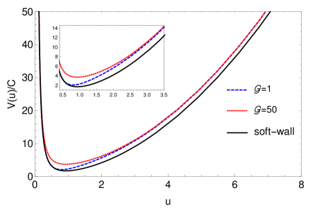
Figure 1: The curves of the potential of Eq. (5) for two different values of $\mathcal{G}$ and, for comparison, the curve of the original potential in the soft-wall model Karch:2006pv . The asymptotic behaviours are similar and the main difference between the models lies in the intermediate region.

As expected, the asymptotic behaviors are similar and the main differences between our approach and the original soft-wall model lies in an intermediate region between the UV and IR, as it can be seen in Fig. 1.

2.3 Asymptotic solutions for the scalar field

Once the asymptotic behaviour of the effective potential is known, we can now find the asymptotic solutions of the Schrödinger-like equation (4). The two regimes, UV and IR, are dealt with separately.

To obtain the asymptotic solutions in the UV regime, we first replace the leading terms of the potential from Eq. (10) into Eq. (4), which leads to

$$-\psi^{\prime\prime}(u)+\left(\frac{3}{4u^{2}}+6\,\mathcal{G}^{2}u^{4}\right)\psi(u)=\hat{m}_{s}^{2}\psi(u),\qquad u\to 0.$$ (12)

As this is a second-order differential equation we have two solutions close the boundary

$$\psi(u)=c_{1}u^{-1/2}+c_{2}u^{3/2},\qquad u\to 0.$$ (13)

The first term on the right hand side of (13) is the non-normalizable solution (see Appendix of Ref. Ballon-Bayona:2017sxa for details), while the second term is the normalizable one. As we are uniquely interested in normalizable solutions, we set $c_{1}=0$.

One might be surprised about the fact that the parameter $\mathcal{G}$ does not affect the asymptotic solutions (13). This is because the asymptotic solution of the scalar field $S(z)$ is not affected by a quartic dilaton in the UV. In fact, its contribution is subleading in Eq. (13).

In the deep IR regime the asymptotic behaviour of the potential is given by Eq. (11) and the Schrödinger-like equation (4) reduces to

$$-\psi^{\prime\prime}(u)+u^{2}\psi(u)=\hat{m}_{s}^{2}\psi(u),\qquad u\to\infty.$$ (14)

Hence, the solution that guarantees convergence of the wave function in this region is given by

$$\psi(u)=b_{1}u^{(\hat{m}_{s}^{2}-1)/2}e^{-u^{2}/2},\qquad u\to\infty.$$ (15)

This function, which gives the asymptotic behaviour of the wave function $\psi(u)$ in the IR region, and the solution (13), that represents the asymptotic behaviour of $\psi(u)$ in the UV region, are used below in the search for a full solution of Eq. (4) through numerical methods.

2.4 Analysis of the mass spectrum

As pointed out above, the normalizable solutions of the differential equation (4) are associated to scalar-meson states. We obtain these solutions by solving numerically the Schrödinger-like equation (4) with a shooting method. For the numerical integration, boundary conditions need to be provided. In the present case, we use the near-boundary UV ($u=0$) normalizable solution (13) and its derivative as “initial" conditions, and complement them by imposing regularity of the wave function in the deep IR region. These conditions are satisfied just for a discrete set of values of the mass parameter $\hat{m}_{s}^{2}$. Notice that, alternatively, we might use the asymptotic solution (15) in the IR ($u\to\infty$) and its derivative as “initial" conditions, and require a regular behaviour of the wave function in the UV boundary $u=0$. Both approaches give the same solutions to the eigenvalue problem.

In Table 1 we present the first nine eigenvalues $\hat{m}_{s}^{2}$ for two different values of the parameter $\mathcal{G}$; namely, $\mathcal{G}=1$ and $\mathcal{G}=50$. These particular values are chosen arbitrarily and their separation is taken large enough to clearly display the dependence of the mass spectrum on such a parameter.

$n$	0	1	2	3	4	5	6	7	8	9
$\hat{m}_{s}^{2}(\mathcal{G}=1)$	4.84	9.16	13.31	17.40	21.46	25.51	29.55	33.57	37.60	41.62
$\hat{m}_{s}^{2}(\mathcal{G}=50)$	5.99	9.99	13.99	17.99	21.99	25.99	29.99	33.99	37.99	41.99

Table 1: The mass spectrum of scalar mesons at zero temperature for two different values of the dimensionless parameter $\mathcal{G}$. The masses are dimensionless.

These results show that the lower excited states are more sensitive to the change of the parameter $\mathcal{G}$ than the higher excited states. To make this fact transparent, we plot the data of Table 1 in Fig. 2, where the differences among the two spectra at low masses is clearly seen. For comparison, let us mention the previous results found in the original soft-wall model Karch:2006pv ; Vega:2008af ; Colangelo:2008us , whose mass spectrum has the closed form

$$\hat{m}_{s}^{2}=(4\,n+6),\qquad n=0,1,2,\cdots\,.$$ (16)

Numerical fits to our results yield the following expressions:

$$\begin{split}\hat{m}_{s}^{2}(\mathcal{G}=1)=&4.05\,n+5.17,\qquad\;n=0,1,2,\cdots\\ \hat{m}_{s}^{2}(\mathcal{G}=50)=&4.00\,n+5.99.\qquad\;n=0,1,2,\cdots\end{split}$$ (17)

As it can be seen, the fit for $\mathcal{G}=50$ approaches the result presented in Eq. (16), while the fit for $\mathcal{G}=1$ is completely different.

Although it is not considered the backreaction of the dilaton on the metric, the condensate is shown to be important for the dynamics of hadron formation in the dual field theory.

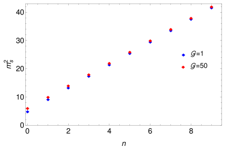
Figure 2: The mass spectrum of scalar mesons at zero temperature for two different values of $\mathcal{G}$.

It is worth mentioning that the spectrum tends to a continuum as the parameter $\mathcal{G}$ goes to zero. In such a limit, it is recovered the problem of a massive scalar field in an AdS background with a constant dilaton.

In the sequence of this work we explore the finite-temperature effects on the mass spectrum due to the presence of the gluon condensate (parameter $\mathcal{G}$).

3 Melting of scalar mesons

3.1 The finite-temperature holographic QCD model

To take into account the finite-temperature effects on the dual field theory, we need to consider a black hole on the gravity side. The standard static black-hole solutions include a horizon function, $f(z)$, in a metric of the form (1). The background geometry we consider here is described by

$$\begin{split}ds^{2}=&g_{mn}dx^{m}dx^{n}\\ =&e^{2A(z)}\left(-f(z)dt^{2}+\frac{1}{f(z)}dz^{2}+\delta_{ij}dx^{i}dx^{j}\right),\end{split}$$ (18)

where $f(z)=1-z^{4}/z_{h}^{4}$, $\delta_{ij}$ is the Kronecker delta and the Latin indices run over the spatial transverse coordinates ($i=1,2,3$). The domain of the holographic coordinate is $0\leq z\leq z_{h}$, where $z_{h}$ indicates the position of the black-hole event horizon. The Hawking temperature of the black hole is given by

$$T=\Bigg{|}\frac{f^{\prime}(z_{h})}{4\pi}\Bigg{|}.$$ (19)

According to the AdS/CFT dictionary, $T$ is also the temperature of the dual thermal field theory.

It is possible to observe the parameter dependence of the confinement/deconfinement temperature (or critical temperature) for gluons by analyzing the free energy of the dual thermal field theory. What is more, the free energy is obtained by calculating the Euclidean on-shell action of the background fields. In the present case, the gravitational action for both cases, the thermal AdS spacetime (1) and the black-hole spacetime (18), are given by Herzog:2006ra

$$\begin{split}\mathcal{S}^{\scriptscriptstyle{\text{Thermal}}}=-\frac{1}{2\kappa^{2}}\int\,d^{5}x\,\sqrt{\tilde{g}}\,e^{-\Phi}\left(\widetilde{R}+\frac{12}{\ell^{2}}\right),\\ \mathcal{S}^{\scriptscriptstyle{\text{BH}}}=-\frac{1}{2\kappa^{2}}\int\,d^{5}x\,\sqrt{g}\,e^{-\Phi}\left(R+\frac{12}{\ell^{2}}\right),\end{split}$$ (20)

where $\kappa$ is the gravitational coupling, and $\tilde{g}_{mn}$ and $g_{mn}$ are the corresponding metrics. To get the Euclidean on-shell action, which is related to the free energy of the dual thermal field theory, we first obtain the Einstein equations (in Ricci form) from (20),

$$\widetilde{R}=-20/\ell^{2},\qquad R=-20/\ell^{2}.$$ (21)

Then, substituting these results into Eq. (20) we get (for the thermal phase)

$$\mathcal{S}^{\scriptscriptstyle{\text{Thermal}}}_{\text{on-shell}}=\frac{4\,V_{3}}{\kappa^{2}\,\ell^{2}}\int_{0}^{\tilde{\beta}}dt\int_{z_{0}}^{\infty}dz\,\sqrt{\tilde{g}}\,e^{-\Phi},$$ (22)

where $V_{3}$ is the three-dimensional transverse volume, $\tilde{\beta}$ corresponds to the period of the Euclidean time $t\sim t+i\tilde{\beta}$, and $z_{0}$ is the UV cutoff which lies close to the boundary. Moreover, doing the same procedure we obtain the on-shell action of the black-hole phase,

$$\mathcal{S}^{\scriptscriptstyle{\text{BH}}}_{\text{on-shell}}=\frac{4\,V_{3}}{\kappa^{2}\,\ell^{2}}\int_{0}^{\beta}dt\int_{z_{0}}^{z_{h}}dz\,\sqrt{g}\,e^{-\Phi},$$ (23)

where the Euclidean time belongs to the interval $0\leq t\leq\beta$, and $z_{0}$ is the UV cutoff located close to the boundary. Furthermore, the temperature $T=1/\beta$ is related to the event-horizon coordinate $z_{h}$ through $\beta=\pi z_{h}$.

The relation between the free energy $F$ and the Euclidean on-shell action is $\beta{F}=S_{\text{on-shell}}$. However, in both cases the on-shell action blows up at the UV cutoff Herzog:2006ra . To avoid these divergences we are going to use a prescription for which matters the difference of the black hole and thermal phases. Thus, the variation of the free energy density $\mathcal{F}=F/V_{3}$ is given by

$$\beta\Delta\mathcal{F}=\lim_{z_{0}\to 0}\frac{1}{V_{3}}\left(\mathcal{S}^{\scriptscriptstyle{\text{BH}}}_{\text{on-shell}}-\mathcal{S}^{\scriptscriptstyle{\text{Thermal}}}_{\text{on-shell}}\right).$$ (24)

Differently from the original soft-wall model Karch:2006pv , here it is not possible to get an analytical expression for $\Delta\mathcal{F}$, so that Eq. (24) must be solved numerically. To guarantee the periodicity in time at the UV cutoff, we set $\tilde{\beta}=\beta\,\sqrt{f(z_{0})}$ Herzog:2006ra . In Fig. 3 we display the numerical results obtained for $\mathcal{G}=1$ (blue line) and $\mathcal{G}=50$ (red line). The results in this figure show the parameter dependence of the difference in the free-energy density. Furthermore, the confinement/deconfinement transition temperature is defined as the temperature for which the free-energy difference is zero. This means that we must solve the equation $\Delta\mathcal{F}(z_{h_{c}})=0$, where the solution $z_{h_{c}}$ is related to the critical temperature as $z_{h_{c}}=1/\pi T_{c}$. Moreover, from Fig. 3 we observe that $z_{h_{c}}(\mathcal{G}=50)<z_{h_{c}}(\mathcal{G}=1)$, which means that $T_{c}(\mathcal{G}=50)>T_{c}(\mathcal{G}=1)$ and, consequently, the critical temperature is a function of the parameter $\mathcal{G}$. The inverse relation, i.e., the temperature dependence of the gluon condensate $\mathcal{G}(T)$, was already reported in the literature; for a discussion in QCD see, for instance, Ref. Boyd:1996ex and in holography Ref. Andreev:2007zv .

To complement this section we analyze the phase transition from the point of view of the degrees of freedom of the systems. A good thermodynamic variable to characterize this issue is the entropy. From the holographic dictionary we may determine the entropy of the dual field theory by calculating the entropy of the gravitational background with the use of the Bekenstein-Hawking formula, i.e., $S=\mathcal{A}/(4G_{5})$, where $\mathcal{A}$ is the event horizon area. As discussed in Ref. BallonBayona:2007vp , the number of degrees of freedom of the deconfined phase is proportional to $N^{2}$ ($N$ is the number of colours), which means that $S\sim N^{2}$, while in the confined phase it is proportional to $N^{0}$, $S\sim N^{0}$. Therefore, the entropy function $S(N)$ has a phase transition because it is discontinuous at $T=T_{c}$.

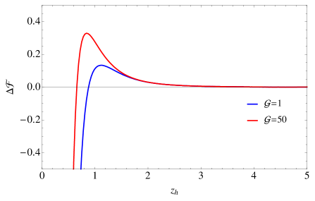
Figure 3: The numerical results for $\Delta\mathcal{F}$ as a function of $z_{h}$ for $\mathcal{G}=1$ (blue line) and $\mathcal{G}=50$ (red line). We have set $C=1$ and $\kappa^{2}\,\ell^{2}=1$.

3.2 Equations of motion for the scalar field

The equation of motion for the scalar field $S(x,z)$ in the black-hole geometry is given by

$$\begin{split}&e^{-3A+\Phi}f\partial_{z}\left[e^{3A-\Phi}f\partial_{z}S(x,z)\right]-\partial^{2}_{t}S(x,z)\\ &+f\left[\delta^{ij}\partial_{i}\partial_{j}-m_{X}^{2}e^{2A}\right]S(x,z)=0.\end{split}$$ (25)

As in section 2, introducing the function $2B=3A-\Phi$ and the tortoise coordinate $\partial_{r_{*}}=-f\,\partial_{z}$ in Eq. (25), and taking the Fourier transform

$$S(x,z)=\int\frac{d^{4}x}{(4\pi)^{4}}e^{-i\omega t+i\mathbf{k}\cdot\mathbf{x}}S(k,x),$$ (26)

we get

$$e^{-2B}\partial_{r_{*}}\left[e^{2B}\partial_{r_{*}}S(k,z)\right]+\left[\omega^{2}-f\left(q^{2}+m_{X}^{2}e^{2A}\right)\right]S(k,z)=0,$$ (27)

where $q^{2}=\mathbf{q}\cdot\mathbf{q}=\mathbf{k}\cdot\mathbf{k}$ is the squared modulus of the spatial part of the four-momentum vector $k^{\mu}$. Finally, to get a Schrödinger-like equation, we introduce the transformation $S=e^{-B}\psi$ and, after some simplifications, we find

$$-\partial_{r_{*}}^{2}\psi(z)+V(z)\psi(z)=\omega^{2}\psi(z),$$ (28)

where the potential is given by

$$V(z)=\partial_{r_{*}}^{2}B+\left(\partial_{r_{*}}B\right)^{2}+f(z)\left(q^{2}+m_{X}^{2}e^{2A}\right).$$ (29)

In the present case, it is helpful to write the explicit form of the tortoise coordinate in terms of the holographic coordinate $z$. Such a relation is given by

$$r_{*}=\frac{z_{h}}{2}\left[-\arctan\left(\frac{z}{z_{h}}\right)+\frac{1}{2}\ln\left(\frac{z_{h}-z}{z_{h}+z}\right)\right].$$ (30)

This coordinate ranges from $r_{*}\to-\infty$ (for $z\to z_{h}$) to $r_{*}=0$ (for $z=0$). An useful form for the effective potential as a function of $z$ is given by

$$V(z)=f(z)\left[\partial_{z}\left(f(z)\partial_{z}B\right)+f(z)\left(\partial_{z}B\right)^{2}+q^{2}+m_{X}^{2}e^{2A}\right],$$ (31)

from which one immediately sees that the potential vanishes at the event horizon.

3.3 Asymptotic solutions for the scalar-meson field

Here we study the asymptotic solutions of the differential equation (28). Since the effective potential (31) vanishes at the horizon, because $f(z_{h})=0$, the solutions for $\psi$ at $z=z_{h}$ are of the plane-wave form

$$\psi\sim\mathfrak{C}\,e^{-i\omega r_{*}}+\mathfrak{D}\,e^{+i\omega r_{*}},$$ (32)

where the first term is a purely ingoing wave, while the second term corresponds to a purely outgoing wave. However, in the neighbourhood of the event horizon the wave functions can also be expressed as power series in $(1-z/z_{h})$, i.e., in series of the form $\psi^{(\pm)}(z)=\sum_{n}a_{n}^{\pm}\left(1-{z}/{z_{h}}\right)^{n\pm i\omega z_{h}^{2}/4}$. After substituting these series into the differential equation (28), we get, up to second order,

$$\begin{split}\psi^{(\pm)}(z)=&\left(1-\frac{z}{z_{h}}\right)^{\pm i\omega z_{h}^{2}/4}\bigg{[}1+a_{1}^{(\pm)}\left(1-\frac{z}{z_{h}}\right)\\ &+a_{2}^{(\pm)}\left(1-\frac{z}{z_{h}}\right)^{2}+\cdots\bigg{]},\end{split}$$ (33)

where the ellipses represent higher-order contributions, and the coefficients are given by

$$\begin{split}a^{(\pm)}_{1}=&\pm\frac{i\,3z_{h}\,\omega}{8}+\frac{\left(3\,C^{2}+C\left(6G+C\,q^{2}\right)z_{h}^{2}+3\,G^{2}\,z_{h}^{4}\right)}{2\left(C+G\,z_{h}^{2}\right)^{2}\left(2\pm i\,\omega\,z_{h}\right)}\\ &-\frac{\,G\left(4\,C+q^{2}\right)\left(2\,C+G\,z_{h}^{2}\right)z_{h}^{4}}{8\left(C+G\,z_{h}^{2}\right)^{2}\left(2\pm i\,\omega\,z_{h}\right)},\\ \end{split}$$

$$\begin{split}a^{(\pm)}_{2}=&\frac{1}{64\left(C+G\,z_{h}^{2}\right)^{4}\left(4\pm i\,\omega\,z_{h}\right)}\bigg{[}-G^{4}z_{h}^{8}\bigg{(}120+24q^{2}\,z_{h}^{2}\\ &\pm 68\,i\,\omega z_{h}-17\omega^{2}z_{h}^{2}\bigg{)}-4\,C\,G^{3}\,z_{h}^{6}\bigg{(}120+24q^{2}\,z_{h}^{2}\\ &+56G\,z_{h}^{4}\pm 68\,i\,\omega\,z_{h}-17\omega^{2}\,z_{h}^{2}\bigg{)}-c^{4}\bigg{(}120+24q^{2}\,z_{h}^{2}\\ &+960\,Gz_{h}^{4}-256G^{2}z_{h}^{8}\pm 68\,i\,\omega z_{h}-17\omega^{2}z_{h}^{2}\bigg{)}\\ &+4C^{3}Gz_{h}^{2}\bigg{(}-120-24q^{2}z_{h}^{2}-408Gz_{h}^{4}+64G^{2}z_{h}^{8}\\ &\mp 68\,i\,\omega z_{h}+17\omega^{2}z_{h}^{2}\bigg{)}+2C^{2}G^{4}z_{h}^{4}\bigg{(}-360-72q^{2}z_{h}^{2}\\ &-448Gz_{h}^{4}+32G^{2}z_{h}^{8}\mp 204\,i\,\omega z_{h}+51\omega^{2}z_{h}^{2}\bigg{)}\bigg{]}\\ &-\frac{a^{(\pm)}_{1}}{16\left(C+Gz_{h}^{2}\right)^{2}\left(4\pm i\,\omega z_{h}\right)}\bigg{[}G^{2}z_{h}^{4}\bigg{(}84+4q^{2}z_{h}^{2}\\ &\pm 30\,i\,\omega z_{h}-3\omega^{2}z_{h}^{2}\bigg{)}\\ &+2C\,Gz_{h}^{2}\left(84+4q^{2}z_{h}^{2}+8Gz_{h}^{4}\pm 30\,i\,\omega z_{h}-3\omega^{2}z_{h}^{2}\right)\\ &+C^{2}\left(84+4q^{2}z_{h}^{2}+32Gz_{h}^{4}\pm 30\,i\,\omega z_{h}-3\omega^{2}z_{h}^{2}\right)\bigg{]}.\end{split}$$

It is worth mentioning that the leading terms in Eqs. (32) and (33) are identical. This can be shown by substituting the tortoise coordinate as a function of $z$ into Eq. (32) and expanding the resulting function in power series of $(1-z/z_{h})$. We prefer to work with Eq. (33) instead of Eq. (32) in the forthcoming sections.

Now we turn attention to the solutions near the boundary $z=0$. The power series expansion of the two independent solutions may be written as

$$\psi^{\scriptscriptstyle{(1)}}(z)= z^{3/2}\left[1+b_{2}\,z^{2}+b_{4}\,z^{4}+b_{6}\,z^{6}+\cdots\right],$$ (34)

$$\psi^{\scriptscriptstyle{(2)}}(z)= z^{-1/2}\left[1+c_{2}\,z^{2}+c_{4}\,z^{4}+c_{6}\,z^{6}+\cdots\right]$$

$$+2d\psi^{\scriptscriptstyle{(1)}}\ln{\left(\frac{z}{z_{h}}\right)},$$ (35)

where the ellipses stand for higher order terms, and the coefficients are given by

$$\begin{split}b_{2}&=\frac{1}{8}\left(q^{2}-\omega^{2}\right),\qquad b_{4}=\frac{3}{8z_{h}^{4}}+\frac{1}{24z_{h}^{2}}b_{2}\left(q^{2}-\omega^{2}\right),\\ b_{6}&=\frac{G^{2}}{8\,C}+\frac{11}{16z_{h}^{6}}b_{2}+\frac{1}{48z_{h}^{4}}\left[-q^{2}+b_{4}\left(q^{2}-\omega^{2}\right)\right],\\ d&=\frac{1}{4}\left(q^{2}-\omega^{2}\right),\qquad c_{2}=\frac{3d}{2z_{h}^{2}}-\frac{1}{z_{h}^{4}\left(q^{2}-\omega^{2}\right)},\\ c_{6}&=\frac{G^{2}}{4\,C}+\frac{3\,c_{2}}{8z_{h}^{6}}+\frac{17d}{48z_{h}^{6}}-\frac{5d}{1152z_{h}^{2}}\left(q^{2}-\omega^{2}\right)^{2}-\frac{q^{2}}{24z_{h}^{4}}.\end{split}$$ (36)

Notice that $\psi^{(1)}$ is a normalizable wave function while $\psi^{(2)}$ is not, since it diverges at the boundary.

In order to calculate the spectral function associated to the scalar mesons (in Sec. 3.6), we follow the same procedure applied in Refs. Miranda:2009uw ; Mamani:2013ssa . First, we write the near-horizon ingoing and outgoing solutions, $\psi^{(-)}$ and $\psi^{(+)}$, as a linear combination of the wave functions close to the boundary,

$$\psi^{\scriptscriptstyle{(\pm)}}=\mathfrak{A}^{\scriptscriptstyle{(\pm)}}\psi^{\scriptscriptstyle{(2)}}+\mathfrak{B}^{\scriptscriptstyle{(\pm)}}\psi^{\scriptscriptstyle{(1)}},$$ (37)

where the coefficients are functions of the wave number and frequency. Second, we may also write the near-boundary solutions as a linear combination of the near-horizon solutions,

$$\begin{split}\psi^{\scriptscriptstyle{(1)}}=&\mathfrak{C}^{\scriptscriptstyle{(1)}}\psi^{\scriptscriptstyle{(-)}}+\mathfrak{D}^{\scriptscriptstyle{(1)}}\psi^{\scriptscriptstyle{(+)}}\,,\\ \psi^{\scriptscriptstyle{(2)}}=&\mathfrak{C}^{\scriptscriptstyle{(2)}}\psi^{\scriptscriptstyle{(-)}}+\mathfrak{D}^{\scriptscriptstyle{(2)}}\psi^{\scriptscriptstyle{(+)}}\,.\end{split}$$ (38)

Doing so, we realized that there is a relation between Eqs. (37) and (38) which can be written in a matrix form (for details about this relation, see Refs. Miranda:2009uw ; Mamani:2013ssa ). To get the spectral function associated to the mesons, we need to know some of the foregoing coefficients ($\mathfrak{A}^{\scriptscriptstyle{(-)}}$ and $\mathfrak{B}^{\scriptscriptstyle{(-)}}$, say) and so, in the sequence of this work, we find numerically the values of these coefficients.

3.4 Analysis of the finite-temperature effective potential

In this subsection we develop a careful analysis of the effective potential (31) and study how it varies with the parameters of the model. First of all, let us write the potential explicitly as a function of the dilaton field $\Phi$, the holographic coordinate $z$ and the black-hole temperature $T$,

$$\begin{split}V=&\frac{3}{4z^{2}}+\left[\frac{3}{2z}+\frac{\Phi^{\prime}(z)}{4}\right]\Phi^{\prime}(z)-\frac{\Phi^{\prime\prime}(z)}{2}+q^{2}+\\ &\bigg{[}\frac{3}{2}-z^{2}q^{2}-\left(1+\frac{z}{2}\Phi^{\prime}(z)\right)z\Phi^{\prime}(z)+z^{2}\Phi^{\prime\prime}(z)\bigg{]}z^{2}\pi^{4}T^{4}\\ &-\frac{1}{2}\bigg{[}\frac{9}{2}+\left(1-\frac{z}{2}\Phi^{\prime}(z)\right)z\Phi^{\prime}(z)+z^{2}\Phi^{\prime\prime}(z)\bigg{]}z^{6}\pi^{8}T^{8}.\end{split}$$ (39)

Now it is helpful to consider some particular cases, beginning by the zero-temperature potential. From Eq. (39), it is clear that we recover the potential (5) with the additional term $q^{2}$ for $T=0$,

$$V(z){\Big{|}}_{T=0}=\frac{3}{4z^{2}}+\left[\frac{3}{2z}+\frac{\Phi^{\prime}(z)}{4}\right]\Phi^{\prime}(z)-\frac{\Phi^{\prime\prime}(z)}{2}+q^{2}.$$ (40)

Thus, by choosing the dilaton as being a quadratic function of the holographic coordinate $z$, we recover previous results from the literature (see, e.g, Refs. Colangelo:2008us ; Bartz:2016ufc ).

Now let us turn off the gluon condensate by taking $G=0$. In doing so, the dilaton field (6) reduces to a constant, i.e., $\Phi(z)=\phi_{0}$, and the potential (39) becomes

$$V(z){\Big{|}}_{G=0}=\frac{3}{4z^{2}}+q^{2}+\left(\frac{3}{2z^{2}}-q^{2}\right)z^{4}\pi^{4}T^{4}-\frac{9}{4}z^{6}\pi^{8}T^{8}.$$ (41)

This is the same potential as that of a pure AdS black hole metric with a massive scalar field.

To implement the numerical analysis of the effective potential, it is convenient to normalize all parameters of the model in order to make them dimensionless. The temperature is normalized by the confinement energy scale as $\widetilde{T}=\pi T/\sqrt{C}$ Miranda:2009uw ; Mamani:2013ssa , and the wavenumber is normalized by the temperature, $\bar{q}=q/\pi T$. We introduce again the dimensionless gluon condensate $\mathcal{G}=G/C^{2}$. The tortoise coordinate is normalized as $\sqrt{C}\,r_{*}$ and the effective potential by $V/C$. For a better visualization of the graphs of the potential, we separate the analysis in two regimes: one for low temperatures ($\widetilde{T}<1$) and another for intermediate and high temperatures ($\widetilde{T}\geq 1$). In Fig. 4 we show the results for intermediate and high temperatures, and two values of the dimensionsless condensate, $\mathcal{G}=1$ (left panel) and $\mathcal{G}=50$ (right panel). These values were chosen arbitrarily and are the same that we used to calculate the spectrum of the scalar mesons at zero temperature presented in Table 1.

By comparing both figures, we observe that the effect of the dimensionless gluon condensate is more relevant for intermediate temperatures; see, for example, the results for $\widetilde{T}=1$. The results for high temperatures are less sensitive to this parameter, as can be seen by comparing the results for $\widetilde{T}=15$.

Another interesting result is the temperature for which the potential well starts to form, as is shown in the small box of Fig. 4. This temperature, that we call as $\widetilde{T}_{w}$, depends on the value of $\mathcal{G}$, such that $\widetilde{T}_{w}=0.782$ for $\mathcal{G}=1$ is greater than $\widetilde{T}_{w}=0.497$ for $\mathcal{G}=50$. As is shown in both figures, for $\widetilde{T}>\widetilde{T}_{w}$ the presence of bound states is not expected due to the absence of a potential well. The potential well starts to form for temperatures smaller than $\widetilde{T}_{w}$. To finish this case, it is noticed the temperature effect in deforming the potential (5), as can be easily seen in the expression (39). For high temperatures, the term $T^{8}$ becomes leading and its effect is visualized in Fig. 4.

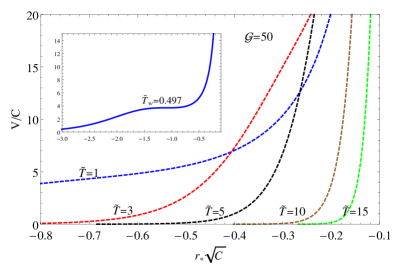
Figure 4: Effective potential with zero wavenumber for $\mathcal{G}=1$ (left panel) and $\mathcal{G}=50$ (right panel) in the regime of intermediate and high temperatures. We also show the potential for $\widetilde{T}=\widetilde{T}_{w}$ in the inset.

The curves for the potential at low temperatures are displayed in Fig. 5. In this regime the potential presents a well and a barrier, with the height of the barrier depending on the temperature. Here we present the results for selected values of temperature such that the maximum value of the potential is equal to the mass of the zero-temperature spectrum displayed in Table 1 and plotted as horizontal lines in this figure. We did this analysis for $\mathcal{G}=1$ (left panel) and $\mathcal{G}=50$ (right panel). Our intention is always to compare with the results at zero temperature obtained in Sec. 2. From Fig. 5 we see that the potential well becomes deeper with the decreasing of the temperature, and this behaviour is the same obtained for scalar glueballs and vector mesons in Refs. Miranda:2009uw ; Mamani:2013ssa . For example, it is possible to have five bound states if the temperature is smaller than $\widetilde{T}=0.121$ (on the left panel of this figure). But since the width of the potential is finite, these bound states have a finite lifetime, and the way they decay depends on the energy they have. For a fixed value of temperature, the higher exited states decay faster that the lower exited states. A careful observation of Fig. 5 shows how the potential (5) is deformed in the regime of low temperatures.

It is known from special relativity that $k_{\mu}k^{\mu}=-m^{2}_{s}$. In the case of a wavevector with a vanishing spatial part, this result reduces to $\omega^{2}=m^{2}_{s}$. This means that, at zero temperature, the frequency is equal to the mass and the potential is shown in Fig. 1. However, in the finite-temperature case, the Lorentz symmetry is broken and such a relation is no longer valid, i.e., $k_{\mu}k^{\mu}\neq-m^{2}_{s}$. As a consequence of it, the frequency acquires an imaginary part that is related to the lifetime of the bound states. This result is supported by the form of the potential in Fig. 5.

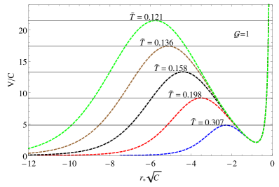
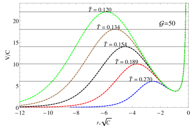
Figure 5: Potential with zero wavenumber for low temperatures for $\mathcal{G}=1$ (left panel) and $\mathcal{G}=50$ (right panel). It is evident how the potential is deformed with the temperature.

From these results is more evident the conclusion that the dimensionless gluon condensate has a strong influence on the low exited states and the higher exited states are less sensitive to this parameter as can be seen by comparing the temperatures in both panels in Fig. 5.

To finish the analysis of the effective potential we write the potential close the boundary in its asymptotic form

$$V=\frac{3}{4z^{2}}+\frac{6\,G^{2}}{C}z^{4}+\cdots\left(\frac{3}{2z^{2}}+8Gz^{2}+\cdots\right)z^{4}\pi^{4}T^{4}+\cdots,$$ (42)

where the ellipses represent higher order contributions in the temperature and holographic coordinate. Or as a functions of the tortoise coordinate this result becomes

$$\begin{split}V=&\frac{3}{4r_{*}^{2}}+\frac{6\,G^{2}}{C}r_{*}^{4}+\cdots\\ &+\left(\frac{9}{5r_{*}^{2}}-\frac{24\,G^{2}}{5C}r_{*}^{4}+\cdots\right)r_{*}^{4}\pi^{4}T^{4}+\cdots,\end{split}$$ (43)

as before, the ellipses represent subleading contributions. In this result is more evident the contribution of the temperature to deform the potential. Differently from the zero temperature case, if we set $\mathcal{G}=0$ we still have bound states at finite temperature, the last term in Eq. (43) guarantee the existence of a potential well.

3.5 Retarded Green function

To find the real-time response in the dual field theory, we need the retarded Green function. The AdS/CFT dictionary allows us to find the correlation functions in the boundary field theory in its Euclidean version Gubser:1998bc ; Witten:1998qj . A prescription to find two-point correlation functions was proposed in Ref. Son:2002sd , and such a prescription is equivalent to the on-shell action re-normalization strategy as developed in Skenderis:2002wp (see also the references therein). It is important to point out that the scalar field $S(x,z)$ satisfies specific boundary conditions: Dirichlet at the AdS boundary and incoming wave at the horizon. These two boundary conditions guarantee that the poles of the retarded Green function are precisely the black-hole QNM spectrum. Here we obtain the two-point function following Ref. Son:2002sd .

Let us start by writing the action (3) in the form

$$\begin{split}\mathcal{S}=&\int dx^{5}\sqrt{-g}e^{-\Phi}S(x,z)\bigg{[}\frac{e^{\Phi}}{\sqrt{-g}}\partial_{m}\left(e^{-\Phi}\sqrt{-g}g^{mn}\partial_{n}\right)\\ &-m_{X}^{2}\bigg{]}S(x,z)-\int dx^{4}e^{-\Phi}\sqrt{-g}g^{zz}S(x,z)\partial_{z}S(x,z)\bigg{|}_{z_{0}}^{z_{h}},\end{split}$$ (44)

where $z_{0}$ is a point close to the boundary and $z_{h}$ is the position of the event horizon. Since the equation of motion is satisfied, the first term in Eq. (44) is zero. Hence, the on-shell action reduces to the surface term

$$\mathcal{S}_{\text{on-shell}}=-\int dx^{4}e^{-\Phi}\sqrt{-g}\,g^{zz}S(x,z)\partial_{z}S(x,z)\bigg{|}_{z_{0}}^{z_{h}}.$$ (45)

After introducing the Fourier transform (26) and decomposing the field as $S(k,z)=S_{0}(k)S_{k}(z)$, where $k$ is the four-momentum, the on-shell action (45) can be written as

$$\mathcal{S}_{\text{on-shell}}=\int\frac{dk^{4}}{(2\pi)^{4}}S_{0}(-k)\mathcal{F}(k,z)S_{0}(k)\bigg{|}_{z_{0}}^{z_{h}},$$ (46)

where

$$\mathcal{F}(k,z)=-e^{-\Phi}\sqrt{-g}\,g^{zz}S_{-k}(z)\partial_{z}S_{k}(z).$$ (47)

This is similar to the result obtained in Ref. Son:2002sd , with the main differences being the presence of the dilaton and the fact that (47) is related to a massive field in the bulk.

Now the asymptotic solutions for the field $S_{k}(z)$, which satisfies an equation of motion in Fourier space identical to Eq. (27), need to be found. Here we also write the generic asymptotic expansion of the solution for a massive scalar bulk field close to the boundary Skenderis:2002wp ,

$$S_{k}(z)=z^{4-\Delta}\left(1+\cdots\right)+z^{4}\left(1+\cdots\right),$$ (48)

where $\Delta$ is the conformal dimension of the operator dual to the scalar field $S$, and the ellipses mean subleading terms. Then, it is possible to write the field as $S_{k}(z)=z^{4-\Delta}f_{k}(z)$, where the function $f_{k}(z)$ satisfies the condition

$$\lim_{z_{0}\to 0}f_{k}(z_{0})=1.$$ (49)

After replacing Eq. (48) into Eq. (47) and using Eq. (49) it follows

$$\mathcal{F}(k,z)=-e^{-\Phi}\sqrt{-g}\,g^{zz}\,z^{4-\Delta}f_{-k}(z)\partial_{z}\left[z^{4-\Delta}f_{k}(z)\right].$$ (50)

We use this result to obtain the retarded Green function following the prescription of Ref. Son:2002sd ,

$$G^{R}(k)=-2\mathcal{F}(k,z).$$ (51)

In order to get the asymptotic solution for the bulk scalar field $S(k,z)$, we use the results of the asymptotic solutions close to the boundary, Eqs. (34) and (35), together with the relations

$$\begin{split}S(k,z)&=e^{-B}\psi(k,z)=\\ &e^{-(3A+\Phi)/2}\left[\mathfrak{A}^{\scriptscriptstyle{(-)}}(\omega,\mathbf{q})\psi^{(2)}(z)+\mathfrak{B}^{\scriptscriptstyle{(-)}}(\omega,\mathbf{q})\psi^{(1)}(z)\right].\end{split}$$ (52)

Now it is easy to get the explicit expression for $f_{k}(z)$ from the relation $S(k,z)=S_{0}(z)\,z^{4-\Delta}\,f_{k}(z)$,

$$f_{k}(z)=z^{1/2}e^{-\Phi/2}\left(\psi^{(2)}(z)+\frac{\mathfrak{B}^{\scriptscriptstyle{(-)}}(\omega,\mathbf{q})}{\mathfrak{A}^{\scriptscriptstyle{(-)}}(\omega,\mathbf{q})}\psi^{(1)}(z)\right),$$ (53)

where we have used $\Delta=3$ and $S_{0}(k)=\mathfrak{A}^{\scriptscriptstyle{(-)}}(\omega,\mathbf{q})$ to guarantee the condition (49). Finally, by using Eqs. (50), (51) and (52), it is obtained the Green function

$$\begin{split}G^{R}(\omega,\mathbf{q})=&2(3c_{2}+2d)\\ &+12\,d\log\left[\frac{z_{0}}{z_{h}}\right]+6\frac{\mathfrak{B}^{\scriptscriptstyle{(-)}}(\omega,\mathbf{q})}{\mathfrak{A}^{\scriptscriptstyle{(-)}}(\omega,\mathbf{q})}+\cdots,\end{split}$$ (54)

where the ellipses denote power corrections in $z_{0}$. After a renormalization process Skenderis:2002wp we take the limit $z_{0}\to 0$ to extract the finite part of (54). The imaginary part of such a result is related to the spectral function (SPF), which is given by

$$\mathcal{R}(\omega,\mathbf{q})=-2\,\text{Im}G^{R}(\omega,\mathbf{q})=-12\,\text{Im}\frac{\mathfrak{B}^{\scriptscriptstyle{(-)}}(\omega,\mathbf{q})}{\mathfrak{A}^{\scriptscriptstyle{(-)}}(\omega,\mathbf{q})}.$$ (55)

It is worth mentioning that the retarded Green function could be obtained using the prescription presented in Ref. Iqbal:2008by . The authors used the canonical momentum associated to the massive scalar field to get this quantity, and showed that their result is consistent with the prescription presented in Ref. Son:2002sd , at least for a massless scalar field. Here we also used the prescription of the canonical momentum for a massive scalar field and obtain the same result as Eq. (54). In the next subsection we present the numerical results for the spectral function (55) and an analysis of its dependence with the temperature and dimensionless gluon condensate.

3.6 Spectral function

3.6.1 General procedure

Here we make a brief summary of the general procedure to obtain the SPFs in holographic QCD. In the present case, the spectral function is given by Eq. (55). The next step is to express the coefficients $\mathfrak{B}^{\scriptscriptstyle{(\pm)}}(\omega,\mathbf{q})$ and $\mathfrak{A}^{\scriptscriptstyle{(\pm)}}(\omega,\mathbf{q})$ in terms of the asymptotic solutions of $\psi$ close to the boundary, as obtained in Sec. 3.3. The idea is to write the solutions and their derivatives as

$$\begin{split}\psi^{\scriptscriptstyle{(a)}}(z)&=\psi^{\scriptscriptstyle{(-)}}(z)\mathfrak{C}^{\scriptscriptstyle{(a)}}+\psi^{\scriptscriptstyle{(+)}}(z)\mathfrak{D}^{\scriptscriptstyle{(a)}},\quad\\ \partial_{z}\psi^{\scriptscriptstyle{(a)}}(z)&=\partial_{z}\psi^{\scriptscriptstyle{(-)}}(z)\mathfrak{C}^{\scriptscriptstyle{(a)}}+\partial_{z}\psi^{\scriptscriptstyle{(+)}}(z)\mathfrak{D}^{\scriptscriptstyle{(a)}},\qquad(a=1,2),\end{split}$$ (56)

where $a=1$ ($a=2$) stands for the normalizable (non-normalizable) solutions. In matrix form, Eq. (56) reads

$$\left(\begin{array}[]{cc}\psi^{\scriptscriptstyle{(a)}}(z)\\ \partial_{z}\psi^{\scriptscriptstyle{(a)}}(z)\end{array}\right)=\left(\begin{array}[]{cc}\psi^{\scriptscriptstyle{(-)}}(z)&\quad\psi^{\scriptscriptstyle{(+)}}(z)\\ \partial_{z}\psi^{\scriptscriptstyle{(-)}}(z)&\quad\partial_{z}\psi^{\scriptscriptstyle{(+)}}(z)\end{array}\right)\left(\begin{array}[]{cc}\mathfrak{C}^{\scriptscriptstyle{(a)}}\\ \mathfrak{D}^{\scriptscriptstyle{(a)}}\end{array}\right).$$ (57)

The aim of this procedure is to get expressions for the coefficients $\mathfrak{D}^{\scriptscriptstyle{(a)}}$ and $\mathfrak{C}^{\scriptscriptstyle{(a)}}$ as functions of the asymptotic solutions. Hence, inverting the matrix product (57) we get the desired result. To be more specific, we are looking for the ratio

$$\frac{\mathfrak{D}^{\scriptscriptstyle{(2)}}}{\mathfrak{D}^{\scriptscriptstyle{(1)}}}=\frac{\psi^{\scriptscriptstyle{(2)}}\partial_{z}\psi^{\scriptscriptstyle{(-)}}-\psi^{\scriptscriptstyle{(-)}}\,\partial_{z}\psi^{\scriptscriptstyle{(2)}}}{\psi^{\scriptscriptstyle{(1)}}\partial_{z}\psi^{\scriptscriptstyle{(-)}}-\psi^{\scriptscriptstyle{(-)}}\,\partial_{z}\psi^{\scriptscriptstyle{(1)}}},$$ (58)

since there is a connection between the coefficients $\mathfrak{D}^{\scriptscriptstyle{(1)}}$, $\mathfrak{D}^{\scriptscriptstyle{(2)}}$ and $\mathfrak{B}^{\scriptscriptstyle{(-)}}$, $\mathfrak{A}^{\scriptscriptstyle{(-)}}$, given by

$$\frac{\mathfrak{B}^{\scriptscriptstyle{(-)}}}{\mathfrak{A}^{\scriptscriptstyle{(-)}}}=-\frac{\mathfrak{D}^{\scriptscriptstyle{(2)}}}{\mathfrak{D}^{\scriptscriptstyle{(1)}}}.$$ (59)

With the analytic expressions in hand, we use the asymptotic solutions (34) and (35) as “initial” conditions and solve numerically the Schrödinger-like equation (28) from a point close to the boundary $z=z_{\epsilon}$ up to a point close to the horizon $z_{nh}=z_{h}-z_{\epsilon}$, where $z_{\epsilon}$ is a sufficiently small positive number, e.g., $z_{\epsilon}=0.001$.

3.6.2 Numerical results

Here we present and discuss some numerical results obtained following the general procedure explained previously. Firstly, we calculate the spectral functions by setting $\mathbf{q}=0$. This means that the spatial components of the momentum are neglected, so that the four-momentum is given by $k^{\mu}=(\omega,\mathbf{0})$. Hence, the bound states in the field theory do not present spatial displacement.

Figure 6 shows the numerical results for the spectral function in the low temperatures regime for $\mathcal{G}=1$ (left panel) and $\mathcal{G}=50$ (right panel).

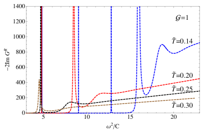
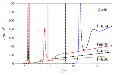
Figure 6: Spectral functions with zero wavenumber in the low-temperature regime for $\mathcal{G}=1$ (left panel) and $\mathcal{G}=50$ (right panel). The number of peaks decreases with the temperature in both cases.

Each curve in a given panel is drawn for a given temperature, as specified in the figure. The curves show several sharpen peaks, and the numerical data around each peak fit well a Breit-Wigner function Fujita:2009ca ; Miranda:2009uw ; Colangelo:2009ra ; Mamani:2013ssa ; Bartz:2016ufc

$$\mathfrak{R}(\omega,\mathbf{0})=\frac{\mathcal{A}\,\omega^{\,\mathfrak{b}}}{\left(\omega-{\omega}_{\scriptscriptstyle{0}}\right)^{2}+\Gamma^{2}}\,,$$ (60)

where $\omega_{\scriptscriptstyle{0}}$ is the position of the peak, $\Gamma$ is the half-width of the curve around the peak, and $\mathcal{A}$ and $\mathfrak{b}$ are constants that can be determined by fitting the numerical data in each case. The peaks are interpreted as quasiparticle states.

The position of each curve peak in Fig. 6 is related to the mass of the corresponding quasiparticle state, while the half-width of the peak is related to the inverse of the quasiparticle lifetime. For instance, in the case $\mathcal{G}=1$ the mass at zero temperature, cf. Table 1, for the fundamental state is $m^{2}=4.84\,C$, and it is possible to get the position of the first peak at $\omega^{2}_{\scriptscriptstyle{0}}=4.78\,C$ for the finite temperature $\widetilde{T}=0.2$. Repeating the same comparison in the case $\mathcal{G}=50$ we get $m^{2}=5.99\,C$ and $\omega^{2}_{\scriptscriptstyle{0}}=5.90\,C$ for $\widetilde{T}=0.2$. The difference between $m^{2}$ and $\omega_{0}^{2}$ depends on the temperature for fixed $\mathcal{G}$, i.e., $\Delta m^{2}(\widetilde{T})=m^{2}-\omega^{2}_{\scriptscriptstyle{0}}$. Note that this difference is positive for nonzero temperature. However, at zero temperature the spectral function reduces to delta functions with peaks located at the values of the masses presented in Table 1. In such a limit the difference is zero, i.e., $\Delta m^{2}(0)=0$. When the temperature is introduced the peaks acquire a width as it can be seen in Fig.6. As the temperature increases the width of the peaks increases while the position of the peaks are shifted. We also see the number of peaks decreasing as the temperature increases, signalling the melting of the quasiparticle states.

In Ref. Fujita:2009ca the SPFs for scalar mesons were obtained by using the soft-wall model. The position of the first peak obtained for $\widetilde{T}=0.22$ is at $\omega^{2}_{\scriptscriptstyle{0}}=5.85\,C$. In order to compare to our results, we have calculated the SPFs for this temperature, but we do not show the corresponding graphics here. For $\mathcal{G}=1$ the first peak is localized at $\omega^{2}_{\scriptscriptstyle{0}}=4.75\,C$, while for $\mathcal{G}=50$ it is localized at $\omega^{2}_{\scriptscriptstyle{0}}=5.85\,C$. From these results we observe, again, that the results of the soft-wall model are obtained when the value of the parameter $\mathcal{G}$ is large, just as we observed when the zero-temperature spectrum was calculated, cf. Sec. 2.4.

Additionally, the results shown in Fig. 6 are in agreement with the results obtained from the effective potential in Fig. 5. For instance, in the analysis of the potential it was shown the possible existence of two quasiparticle states for $\widetilde{T}=0.2$ in both cases, $\mathcal{G}=1$ and $\mathcal{G}=50$. This is also supported by the SPFs where there are two peaks for the same temperature. The effect of the parameter $\mathcal{G}$ shows up in shifting the position, height, and width of the peaks (see Fig. 7). In other words, the position, height and width of the peaks are functions of $\widetilde{T}$ and $\mathcal{G}$ too, i.e., $\omega_{\scriptscriptstyle{0}}(\widetilde{T},\mathcal{G})$ and $\Gamma(\widetilde{T},\mathcal{G})$.

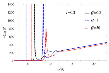
Figure 7: The spectral functions with zero wavenumber for $\mathcal{G}=0.2$, $\mathcal{G}=1$ and $\mathcal{G}=50$. These results were obtained for $\widetilde{T}=0.2$.

It is noticed that the parameter $\mathcal{G}$ shifts $\omega_{\scriptscriptstyle{0}}$ to more energetic states, while the width of the peak increases. To finish the analysis of the SPFs we consider a finite spatial momentum in the above results, i.e., $\mathbf{q}\neq 0$. Hence, the quasiparticle states have spatial displacement and therefore become more energetic. The results for this case are presented in Fig. 8 for $\mathcal{G}=1$ (left panel) and $\mathcal{G}=50$ (right panel). The addition of spatial momentum shifts the position of the peaks to more energetic states, and the half-widths also increase as the spatial momentum increases. This means that more energetic states, i.e., quasiparticles with higher momenta, have shorter lifetime and therefore they melt faster than the low energy states.

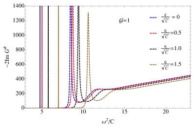
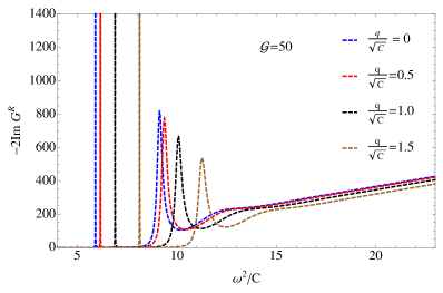
Figure 8: Spectral functions with different wavenumber values for $\mathcal{G}=1$ (left panel) and $\mathcal{G}=50$ (right panel), in both cases we set $\widetilde{T}=0.2$.

4 Quasinormal modes

In this section we present the results for the spectrum of black-hole quasinormal modes (QNMs) associated to the scalar field $S(x,z)$. The field backreaction on the black-hole geometry is neglected, so that the scalar field is considered as a probe field.

4.1 Power series method

The standard procedure to use the power series method is to transform the second-order eigenvalue problem, characterized by a dependence in $\omega^{2}$, into a differential equation which depends linearly in $\omega$ Horowitz:1999jd . To do that we introduce the following transformation into the Schrödinger-like equation (28)

$$\psi(z)=e^{-i\omega r_{*}}\varphi(z).$$ (61)

After replacing $dz/dr_{*}=-f(z)$ and simplifying, the following equation shows up

$$f(z)\,\varphi^{\prime\prime}(z)+\big{[}2i\omega+f^{\prime}(z)\big{]}\varphi^{\prime}(z)-\frac{V(z)}{f(z)}\,\varphi(z)=0,$$ (62)

where $V(z)$ is given by Eq. (31) and $\varphi(z)$ is a regular function in the interval $[0,z_{h}]$. As in previous sections, we use the wave function behavior near the horizon to label the two independent solutions of Eq. (62) by $\varphi^{(+)}$ (the outgoing wave) and $\varphi^{(-)}$ (the ingoing wave). Now we write the solution for $\varphi^{(-)}$ as a power series expansion around the horizon $z=z_{h}$,

$$\varphi^{\scriptscriptstyle{(-)}}(z)=\sum_{n=0}^{\infty}\,a^{\scriptscriptstyle{(-)}}_{n}\left(1-\frac{z}{z_{h}}\right)^{n},$$ (63)

where the coefficients $a_{n}$ are functions of the parameters of the model and, by convention, we set $a_{0}=1$. The spectrum of QN frequencies is obtained by imposing Dirichlet condition at the boundary, i.e., $\varphi^{\scriptscriptstyle{(-)}}(0)=0$, which is equivalent to solve the following recursive equation

$$\sum_{n=0}^{\infty}\,a^{\scriptscriptstyle{(-)}}_{n}(\omega,q,T,C,G)=0.$$ (64)

This method, first employed in Ref. Horowitz:1999jd , works well for large AdS black holes, i.e., for high temperatures. For low temperatures the numerical convergence gets poor, as it was previously noticed in holographic QCD models for scalar glueballs and vector mesons Miranda:2009uw ; Mamani:2013ssa .

4.2 Breit-Wigner method

As commented previously, it is known that the power series method is not reliable to find QN frequencies in the regime of low temperatures. In such a regime, however, the form of the effective potential (cf. Sec. 3.4) allow us to apply a resonance method to obtain the black-hole QN frequencies. In this subsection we use the Breit-Wigner (resonance) method to calculate the frequencies associated to the scalar-field perturbations. This method was applied for the very first time in Ref. Berti:2009wx to compute QNMs of small Schwarzschild-AdS black holes. In the context of holographic QCD this numerical method was previously applied in Refs. Miranda:2009uw ; Mamani:2013ssa .

Now we make a brief summary of the Breit$-$Wigner method; see Refs. Berti:2009wx ; Miranda:2009uw ; Mamani:2013ssa and references therein for details. Firstly, we write the normalizable solution $\psi^{\scriptscriptstyle{(1)}}$ of the Schrödinger-like equation (28), in the neighborhood of the horizon, as

$$\begin{split}\psi^{\scriptscriptstyle{(1)}}&=\mathfrak{C}^{\scriptscriptstyle{(1)}}e^{-i\omega r_{*}}+\mathfrak{D}^{\scriptscriptstyle{(1)}}e^{+i\omega r_{*}}\\ &=\alpha\,(\omega)\cos(\omega r_{*})-\beta\,(\omega)\sin(\omega r_{*})\,.\end{split}$$ (65)

The ingoing-wave boundary condition at the horizon requires the vanishing of the coefficient $\mathfrak{D}^{\scriptscriptstyle{(1)}}$. This means that, for $\omega$ close to the QN frequency, we might approximate it as $\mathfrak{D}^{\scriptscriptstyle{(1)}}\sim(\omega-\omega_{\scriptscriptstyle{\text{QNM}}})$, where $\omega_{\scriptscriptstyle{\text{QNM}}}=\omega_{\scriptscriptstyle{R}}-i\,\omega_{\scriptscriptstyle{I}}$. Notice also that, from Eq. (65), $\mathfrak{C}^{\scriptscriptstyle{(1)}}=\mathfrak{D}^{{\scriptscriptstyle{(1)}}\,*}$. Taking this information into consideration we obtain

$$\alpha^{2}+\beta^{2}=4\,\mathfrak{C}^{\scriptscriptstyle{(1)}}\,\mathfrak{D}^{\scriptscriptstyle{(1)}}\approx\text{const.}\times\left[(\omega-\omega_{\scriptscriptstyle{R}})^{2}+\omega_{\scriptscriptstyle{I}}^{2}\right],$$ (66)

where $\omega$ is a real parameter. Hence, the real par of $\omega$ can be obtained by minimizing Eq. (66). In turn, the imaginary part of the frequency is obtained by fitting a parabola to Eq. (66). Alternatively it is possible to obtain the imaginary part of the frequency using the following formulas Berti:2009wx ; Miranda:2009uw ; Mamani:2013ssa

$$\omega_{\scriptscriptstyle{I}}=-\frac{\alpha}{\partial_{\omega}\beta}=\frac{\beta}{\partial_{\omega}\alpha}.$$ (67)

In the numerical analysis below, we take into consideration the value of the imaginary part obtained using these two procedures.

4.3 Pseudo-spectral method

The pseudo-spectral method boyd:2001 is used here to solve the linear eigenvalue problem (62). In this method, the regular solution of Eq. (62) is expanded in terms of cardinal functions $C_{j}(z)$. To do that we first make the substitution $\varphi(z)=(z/z_{h})^{3/2}\,g(z)$, such that $g(z)$ is a regular function in the interval $[0,z_{h}]$. The differential equation for $g(z)$, which follows from Eq. (62), can be written in the form

$$\begin{split}&\lambda_{2}(z,q,T,C,G)\,g^{\prime\prime}(z)+\lambda_{1}(z,\omega,q,T,C,G)\,g^{\prime}(z)\\ &+\lambda_{0}(z,\omega,q,T,C,G)\,g(z)=0,\end{split}$$ (68)

where $\lambda_{2},\lambda_{1}$ and $\lambda_{0}$ are linear polynomials in $\omega$. Now we expand the regular function $g(z)$ as

$$g(z)=\sum_{j=0}^{N}\,g(z_{j})\,C_{j}(2z/z_{h}-1),$$ (69)

where $C_{j}(2z/z_{h}-1)$ are the Chebyshev polynomials, and the collocation points are chosen to be the Chebyshev-Gauss-Lobatto grid boyd:2001 :

$$z_{j}=\frac{z_{h}}{2}\left[1-\cos\left(\frac{j\,\pi}{N}\right)\right].$$ (70)

By substituting (69) into (62) it gives the matrix form of the eigenvalue problem,

$$(A+\omega\,B)\cdot\vec{g}=0,$$ (71)

where $A$ and $B$ are $(N+1)\times(N+1)$ matrices and $\vec{g}$ is a $(N+1)-$dimensional vector with components $g_{j}=g(z_{j})$, $j=0,\,1,...,N$. It is not difficult to implement numerically a code to solve Eq. (71).

It is worth mentioning that the pseudo-spectral method inevitably leads to the emergence of spurious solutions that do not have any physical meaning. To eliminate the spurious solutions we use the fact that the relevant QN frequencies do not depend on the number of Chebyshev polynomials being considered in Eq. (69).

4.4 Numerical results

Here we present and discuss the numerical results for the QN frequencies obtained with the use of the foregoing methods. Firstly, in Fig. 9 we display the overlap of the results obtained using the power series, pseudo-spectral and Breit-Wigner methods for different values of the parameter $\mathcal{G}$ and setting $q=0$. The results of the real and imaginary parts of the QN frequency for $\mathcal{G}=1$ are displayed in the top panels. In this figure the numerical results for the fundamental mode ($n=0$) and $\widetilde{T}^{2}\ll 1$ were obtained with the Breit-Wigner method, since the power series method has a poor convergence in this regime. The opposite occurs as the temperature increases: the Breit-Wigner method has a poor convergence while the power series method has a good one for high temperatures. Such an overlap of results obtained with both methods, in the intermediate regime of temperatures, is only achieved in the case of the fundamental mode ($n=0$). For higher modes ($n\geq 1$), there are some values of the temperature for example, $0.04\leq\widetilde{T}^{2}\leq 0.08$, for which none of these two methods provides solutions. To fill these empty regions of the spectrum, we use the pseudo-spectral method, which has a good convergence from the low- to the high-temperature regimes. For some values in the intermediate regime of temperatures all the employed methods work well and it is possible to compare the numerical results obtained using the three methods.

In the left panels of Fig. 9, we present the real part of the QN frequencies as a function of the temperature. We observe that $\widetilde{\omega}_{R}$ approaches the values displayed in Table 1, i.e., the spectrum at zero temperature, $\widetilde{\omega}^{2}_{\scriptscriptstyle{R}}=(4.05\,n+5.17)$ for $\mathcal{G}=1$ and $\widetilde{\omega}^{2}_{\scriptscriptstyle{R}}=(4.00\,n+5.99)$ for $\mathcal{G}=50$, with $n=0,\,1,\,2,...\,$. We also observe a smooth transition between the characteristic behaviours of low to high temperature regimes. In particular, $\widetilde{\omega}_{R}$ scales linearly with $\widetilde{T}$ for high values of the temperature, i.e., $\widetilde{\omega}_{R}\propto\widetilde{T}$. It is important to point out that, in the low temperature regime, the QN frequencies may be interpreted as quasiparticle states, since in this case the quality factor is greater than one, i.e., $Q=\omega_{R}/(2\omega_{I})\gg 1$.

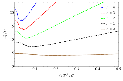
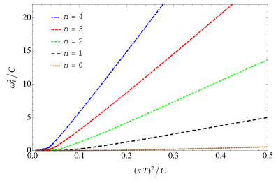
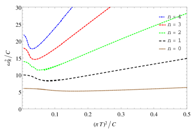
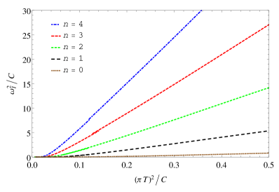
Figure 9: The first five QN frequencies obtained using the Breit-Wigner, power series, and pseudo-spectral methods. The top panels show the results obtained for $\mathcal{G}=1$, while the bottom panels show the results for $\mathcal{G}=50$.

In comparison to the real part, the imaginary part of the QN frequencies has a different behavior as a function of the temperature: it increases monotonically with the temperature, cf. the right panels in Fig. 9. In the limit of zero temperature, the imaginary part of the frequencies becomes zero, which means that the lifetime $\tau=1/\omega_{I}$ of the (quasi)particle states becomes arbitrarily large. For intermediate temperatures, $\widetilde{\omega}_{I}$ follows the power law $\widetilde{\omega}_{I}\propto\widetilde{T}^{\alpha}$, where the exponent $\alpha$ can be obtained by fitting the numerical results, while for high temperatures it grows linearly with the temperature.

Additionally, we plot on the complex plane $\widetilde{\omega}_{R}\times\widetilde{\omega}_{I}$ the numerical results obtained with the pseudo-spectral method, see Fig. 10. It is worth mentioning that in the case without dilaton, i.e., for, $\mathcal{G}=0$, the results are identical to those found in Ref. Nunez:2003eq . We may observe in Fig. 10 and also in Table 2 the changes in the structure of poles as a function of the parameter $\mathcal{G}$.

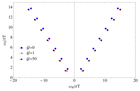
Figure 10: The the numerical results obtained using the pseudo-spectral method for selected values of the parameter $\mathcal{G}$.

	$\mathcal{G}=0$		$\mathcal{G}=1$		$\mathcal{G}=50$
$n$	$\omega_{\scriptscriptstyle{R}}/\pi T$	$\omega_{\scriptscriptstyle{I}}/\pi T$	${\omega}_{\scriptscriptstyle{R}}/\pi T$	${\omega}_{\scriptscriptstyle{I}}/\pi T$	${\omega}_{\scriptscriptstyle{R}}/\pi T$	${\omega}_{\scriptscriptstyle{I}}/\pi T$
0	$\pm 2.19882$	1.75953	$\pm 2.50343$	1.33438	$\pm 2.90009$	1.41878
1	$\pm 4.21190$	3.77488	$\pm 4.59205$	3.32799	$\pm 4.80058$	3.41043
2	$\pm 6.21554$	5.77725	$\pm 6.66143$	5.34384	$\pm 6.79148$	5.43619
3	$\pm 8.21716$	7.77808	$\pm 8.72617$	7.37164	$\pm 8.82048$	7.47670
4	$\pm 10.21806$	9.77847	$\pm 10.79386$	9.40469	$\pm 10.87444$	9.51944
5	$\pm 12.21861$	11.77870	$\pm 12.86690$	11.43744	$\pm 12.94509$	11.55560

Table 2: Numerical results of the first six quasinormal frequencies obtained using the pseudo-spectral method for $\widetilde{q}=0$ and selected values of temperature, by setting $\mathcal{G}=0$, $\mathcal{G}=1$ and $\mathcal{G}=50$.

For completeness we compare the results obtained using the three numerical methods employed in this work. In Table 3 we display some selected values of the QN frequencies. We observe that the Breit$-$Wigner and the pseudo-spectral methods work well for low temperatures, while the power series method has a poor convergence in this regime. Moreover, we observe that the Breit$-$Wigner method no longer works well as the temperature increases, whereas the power series, in contrast, has a good convergence for high temperatures. It is interesting to note that the pseudo-spectral method has a good convergence for all the temperatures in Table 3. Hence, the pseudo$-$spectral method is an alternative to both the Breit$-$Wigner and the power series methods. In general, the application of each method depends on the subject in which the research is focused. Finally, we realized that the convergence of these methods gets poor as the overtone number increases, $n=2,3,\cdots\,$.

	Breit-Wigner		Power Series		Pseudo-spectral
$\widetilde{T}^{2}$	$\widetilde{\omega}_{\scriptscriptstyle{R}}^{2}$	$\widetilde{\omega}_{\scriptscriptstyle{I}}^{2}$	$\widetilde{\omega}_{\scriptscriptstyle{R}}^{2}$	$\widetilde{\omega}_{\scriptscriptstyle{I}}^{2}$	$\widetilde{\omega}_{\scriptscriptstyle{R}}^{2}$	$\widetilde{\omega}_{\scriptscriptstyle{I}}^{2}$
0.080	5.57034	1.33179$\times 10^{-3}$	5.54109	8.11086$\times 10^{-4}$	5.54446	1.23705$\times 10^{-3}$
0.075	5.60471	6.77532$\times 10^{-4}$	5.59656	3.86904$\times 10^{-4}$	5.59037	6.48688$\times 10^{-4}$
0.060	5.74268	3.02717$\times 10^{-5}$	5.75693	3.16718$\times 10^{-5}$	5.74187	3.01802$\times 10^{-5}$
0.030	5.94323	4.34800$\times 10^{-15}$	-	-	5.94323	4.34811$\times 10^{-15}$
0.020	5.97205	1.36357$\times 10^{-19}$	-	-	5.97205	1.08006$\times 10^{-26}$
0.010	5.98859	2.27076$\times 10^{-19}$	-	-	5.98859	1.93069$\times 10^{-27}$

Table 3: Numerical results of the first quasinormal mode for $\widetilde{q}=0$, $\mathcal{G}=50$ and selected values of temperature.

4.5 Comments on the imaginary part of the QN frequencies

To finish this section we consider some interesting features about the imaginary part of the QN frequencies. In particular, we are interested here in the relation between the equilibration timescale $\tau\propto 1/\omega_{I}$ and the temperature of the dual thermal field theory. Let us start with the relation between the imaginary part of the frequency and the radius of the event horizon, $r_{+}$. In the case of the global Schwarzschild-AdS black hole, it was found in Ref. Horowitz:1999jd that the imaginary part of the scalar-field QN frequency scales with the horizon area for small black holes, i.e., $\omega_{I}\propto\mathcal{A}$, where $\mathcal{A}$ is the area of the black-hole event horizon. Moreover, in a five-dimensional spacetime, the area of a spherical region of radius $r_{+}$ is such that $\mathcal{A}\propto r_{+}^{3}$. This behavior was also confirmed with the use of the Breit-Wigner method in Ref. Berti:2009wx for the scalar-field perturbations (see Ref. Wang:2014eha for an extension of these results to arbitrary dimensions). In the case of large black holes, the imaginary part of the QN frequency scales with the horizon radius, $\omega_{I}\propto r_{+}$. Hence, we may construct an interpolation function which recovers the asymptotic behaviors of $\omega_{I}$. One possibility is

$${\omega}_{I}=\frac{a_{1}\,r_{+}^{3}}{b_{1}+c_{1}\,r_{+}^{2}},$$ (72)

where the constants $a_{1}$, $b_{1}$ and $c_{1}$ may be determined by fitting this function to the numerical results Horowitz:1999jd .

The foregoing discussion is valid for Schwarzschild AdS black holes with spherical geometry. Now, we address a similar analysis for the planar AdS black hole, which is the case we are dealing with in this work. As a matter of fact, our numerical results displayed in Fig. 9 show a linear behavior in the regime of large temperatures, $\widetilde{\omega}_{I}\propto\widetilde{T}$. This relation, in turn, is no longer valid in the regime of low temperatures. However, we know (from Fig. 9) that the imaginary part of the QN frequencies vanishes in the zero temperature limit, so that the relation must be in the form $\widetilde{\omega}_{I}\propto\widetilde{T}^{\alpha}$, where $\alpha$ must be a positive number. Then we construct an interpolation function as

$$\widetilde{\omega}_{I}=\frac{a\,\widetilde{T}^{\alpha}+b\,\widetilde{T}^{\alpha+1}}{c+\,\widetilde{T}^{\alpha-1}},$$ (73)

where the constants may be determined by fitting this function with our numerical results. Hence, the best fit we have found in the interval of temperatures $0.01\leq\widetilde{T}^{2}\leq 0.5$ is for the values: $a=95.0\times 10^{-3}$, $b=1.37$, $c=15.3\times 10^{-4}$ and $\alpha=7.60$. This fit was done for the case $\mathcal{G}=1$.

5 Dispersion relations

Here we study the momentum dependence of the QN frequencies for selected values of the temperature. These are the dispersion relations $\{\omega_{R}(q),\omega_{I}(q)\}$ for the scalar field.

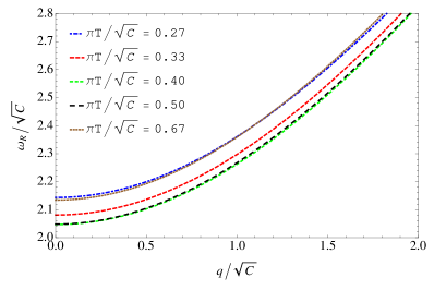
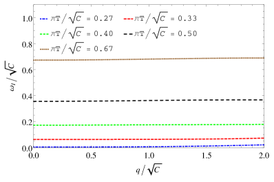
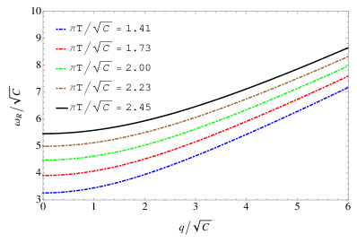
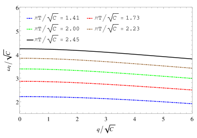
Figure 11: Dispersion relations for low temperatures (top panels), intermediate and high temperatures (bottom panels) for $\mathcal{G}=1$.

The dispersion relations for the first five QN frequencies, for selected values of temperature and setting $\mathcal{G}=1$, are displayed in Fig. 11. The results for low temperatures are displayed in the top panels, while the results for intermediate and high temperatures are displayed in the bottom panels of the same figure. The obtained frequencies for low temperatures are consistent with the results presented in Sec. 3.6, where the real part of the frequency, i.e., the location of the peaks of the SPFs, increases with the wavenumber, for the same temperature, cf. Fig. 6. Moreover, the imaginary part of the frequency, i.e., the width of the peaks in Fig. 6, also increases, but very slowly, with the wavenumber. This behaviour holds for low temperatures, where quasiparticle excitations are present in the quark-gluon plasma.

The results for intermediate and high temperatures are displayed in the bottom panels of Fig. 11. The real part of the frequencies grows with the wavenumber, while the imaginary part decreases. It is worth pointing out that previous studies in the literature have calculated QN frequencies of massive scalar fields without a dilaton field, and the results have a similar behavior for the imaginary part of the frequencies, i.e., $\omega_{I}$ decreasing with $q$ (see for instance Ref. Nunez:2003eq ). In general, for intermediate and large temperatures, this kind of behaviour seems to be an universal property and is shared by QNMs in several gravitational theories (see, e.g., the reviews of Refs. Berti:2009kk ; Konoplya:2011qq and the references therein).

A second particular case is shown in Fig. 12, where we plot the QN frequencies as functions of the normalized wavenumber $\widetilde{q}$ for $\mathcal{G}=50$. By comparing the Figs. 11 and  12, we observe that the real part of the frequencies calculated for $\mathcal{G}=50$ is larger than the one calculated for $\mathcal{G}=1$ (for the same low temperature). The same is true for the imaginary part of the frequencies, $\omega_{I}(\mathcal{G}=50)>\omega_{I}(\mathcal{G}=1)$, which means that the thermalization timescales $\tau=1/\omega_{I}$ become smaller as the value of the parameter $\mathcal{G}$ increases (see also Table 4). Observing carefully the top right panel of Fig. 12 we realized that for $\widetilde{T}\geq 0.40$ the imaginary part of the frequency decreases slightly, and this is different from the corresponding result for $\mathcal{G}=1$. On the other hand, for higher values of temperature, the behavior of the imaginary part of the QN frequencies is the opposite, $\omega_{I}(\mathcal{G}=50)<\omega_{I}(\mathcal{G}=1)$, which means that the thermalization timescales are shorter for small $\mathcal{G}$ (see also Table 5).

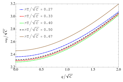
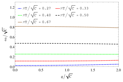
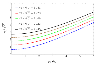
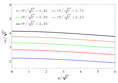
Figure 12: Dispersion relations for low temperatures (top panels), intermediate and high temperatures (bottom panels) for $\mathcal{G}=50$.

To explicitly verify the dependence of the QN frequencies on the temperature we show in Tables 4 and 5 some selected numerical results for a fixed wavenumber value $\widetilde{q}=1$, and the same two values of parameter $\mathcal{G}$ of Figs. 11 and 12. The dependence on the temperature is seen by comparing the two tables, while the dependence on the values of the parameter $\mathcal{G}$ is seen within each table.

	$\mathcal{G}=1$		$\mathcal{G}=50$
$\widetilde{T}$	$\widetilde{\omega}_{\scriptscriptstyle{R}}$	$\widetilde{\omega}_{\scriptscriptstyle{I}}$	$\widetilde{\omega}_{\scriptscriptstyle{R}}$	$\widetilde{\omega}_{\scriptscriptstyle{I}}$
0.27	2.36056	0.00611	2.56318	0.02563
0.33	2.29729	0.06309	2.50387	0.11104
0.40	2.26243	0.17505	2.48310	0.24863
0.50	2.26746	0.36195	2.52008	0.46387
0.67	2.35912	0.68080	2.66534	0.80273

Table 4: Numerical results of the first quasinormal mode for $\widetilde{q}=1$ and low temperatures.

	$\mathcal{G}=1$		$\mathcal{G}=50$
$\widetilde{T}$	$\widetilde{\omega}_{\scriptscriptstyle{R}}$	$\widetilde{\omega}_{\scriptscriptstyle{I}}$	$\widetilde{\omega}_{\scriptscriptstyle{R}}$	$\widetilde{\omega}_{\scriptscriptstyle{I}}$
1.41	3.44958	2.20297	3.82511	2.19533
1.73	4.07448	2.84548	4.42452	2.78078
2.00	4.62865	3.36980	4.95030	3.27206
2.23	5.12904	3.82111	5.42478	3.70372
2.45	5.58760	4.22248	5.86061	4.09311

Table 5: Numerical results of the first quasinormal mode for $\widetilde{q}=1$ and high temperatures.

6 Final remarks and conclusion

In this work we have considred the effects of the gluon condensate in the spectrum and melting of scalar mesons in holographic QCD. Additionally, in the gravitational background, we determined the spectrum of QNMs and explore the dependence of such a spectrum on the parameter associated with the gluon condensate. The effects of the gluon condensate were introduced by considering a quartic dilaton in the UV and quadratic in the IR (in order to guarantee confinement and linear Regge trajectories). The results obtained show that the spectrum at zero temperature is sensitive to the value of the energy scale $G$ associated with the condensate. For large values of this parameter we obtain the same spectrum as obtained in the original soft-wall model applied to the case of scalar mesons. On the other hand, when this parameter is zero we recover the problem of an AdS spacetime with constant dilaton field. In this case the conformal symmetry is restored and the spectrum becomes continuum.

The results are more interesting when the gravitational background contains a black hole, since the presence of the black hole implies in a dual field theory at finite temperature. In this case the conformal symmetry is broken by the dilaton and by the temperature. Differently from the zero temperature case, even in the case $G=0$ and the results show a discrete spectrum because the potential has a well due to finite temperature. Our results also show that the potential well depends directly on the dimensionless parameters $\mathcal{G}$ and $\widetilde{T}$. These parameters deform the potential in such a way that there are more trapped quasiparticle states at low temperatures, where the potential has wells (cf. Fig. 5). These results are supported nicely by the spectral functions (cf. 6). In the low-temperature regime, we observe the presence of peaks in the spectral functions, and such peaks disappear when the temperature increases, characterizing the melting of the scalar mesons. We also observe that higher excited quasiparticle states melt faster than low excited states for the same temperature. These effects are enhanced when spatial momentum is taken into account.

We complement this work by calculating the spectrum of black-hole quasinormal modes associated to the scalar-field perturbations. The numerical results show a finite real part of the frequencies in the limit of zero temperature, while the imaginary part becomes zero (cf. Fig. 9). In this limit the QNMs become normal modes. As an additional analysis we have used three numerical techniques to calculate the spectrum, and from a comparison, we realized that they work well in a determinate regime of temperatures and can be used for specific purposes. At the end we present the numerical results and a discussion on the dispersion relations. In all the results obtained in this work we observe the relevance of the parameter $\mathcal{G}$, and how important is to take it into account when studying the melting of scalar mesons in a holographic model for QCD.

- (1) E. V. Shuryak, The QCD vacuum, hadrons and the superdense matter, World Sci. Lect. Notes Phys. 71, 1 (2004); [World Sci. Lect. Notes Phys. 8, 1 (1988)].
- (2) B. Lucini and M. Panero, Prog. Part. Nucl. Phys. 75, 1 (2014).
- (3) M. A. Shifman, A. I. Vainshtein and V. I. Zakharov, Nucl. Phys. B 147, 385 (1979).
- (4) Y. Kim, I. J. Shin and T. Tsukioka, Prog. Part. Nucl. Phys. 68, 55 (2013).
- (5) J. Erlich, Contemp. Phys. 56, no. 2, 159 (2015).
- (6) J. M. Maldacena, Int. J. Theor. Phys. 38, 1113 (1999) [Adv. Theor. Math. Phys. 2, 231 (1998)].
- (7) S. S. Gubser, I. R. Klebanov and A. M. Polyakov, Phys. Lett. B 428, 105 (1998).
- (8) E. Witten, Adv. Theor. Math. Phys. 2, 253 (1998).
- (9) C. Csaki and M. Reece, JHEP 0705, 062 (2007).
- (10) A. Karch, E. Katz, D. T. Son and M. A. Stephanov, Phys. Rev. D 74, 015005 (2006).
- (11) U. Gursoy and E. Kiritsis, JHEP 0802, 032 (2008).
- (12) U. Gursoy, E. Kiritsis and F. Nitti, JHEP 0802, 019 (2008).
- (13) M. Asakawa, T. Hatsuda and Y. Nakahara, Prog. Part. Nucl. Phys. 46, 459 (2001).
- (14) M. Asakawa, T. Hatsuda and Y. Nakahara, Nucl. Phys. A 715, 863 (2003) [Nucl. Phys. Proc. Suppl. 119, 481 (2003)].
- (15) E. Witten, Adv. Theor. Math. Phys. 2 (1998) 505.
- (16) D. T. Son and A. O. Starinets, JHEP 0209, 042 (2002).
- (17) G. Policastro, D. T. Son and A. O. Starinets, JHEP 0209, 043 (2002).
- (18) G. Policastro, D. T. Son and A. O. Starinets, JHEP 0212, 054 (2002).
- (19) J. Noronha and G. S. Denicol, arXiv:1104.2415 [hep-th].
- (20) M. P. Heller, R. A. Janik, M. Spalinski and P. Witaszczyk, Phys. Rev. Lett. 113, no. 26, 261601 (2014).
- (21) R. A. Janik, “AdS/CFT for the early stages of heavy ion collisions,” Nucl. Phys. A 931, 176 (2014).
- (22) E. Berti, V. Cardoso and A. O. Starinets, Class. Quant. Grav. 26, 163001 (2009).
- (23) R. A. Konoplya and A. Zhidenko, Rev. Mod. Phys. 83, 793 (2011).
- (24) L. Da Rold and A. Pomarol, JHEP 0601, 157 (2006).
- (25) T. Gherghetta, J. I. Kapusta and T. M. Kelley, Phys. Rev. D 79, 076003 (2009).
- (26) J. Erlich, E. Katz, D. T. Son and M. A. Stephanov, Phys. Rev. Lett. 95, 261602 (2005).
- (27) A. Ballon-Bayona, H. Boschi-Filho, L. A. H. Mamani, A. S. Miranda and V. T. Zanchin, Phys. Rev. D 97, no. 4, 046001 (2018).
- (28) C. P. Herzog, Phys. Rev. Lett. 98, 091601 (2007).
- (29) A. Vega and I. Schmidt, Phys. Rev. D 78, 017703 (2008).
- (30) P. Colangelo, F. De Fazio, F. Giannuzzi, F. Jugeau and S. Nicotri, Phys. Rev. D 78, 055009 (2008).
- (31) D. Li and M. Huang, JHEP 1311, 088 (2013).
- (32) S. S. Gubser, A. Nellore, S. S. Pufu and F. D. Rocha, Phys. Rev. Lett. 101, 131601 (2008).
- (33) K. A. Olive et al. [Particle Data Group], Chin. Phys. C 38, 090001 (2014).
- (34) G. Boyd and D. E. Miller, hep-ph/9608482.
- (35) O. Andreev, Phys. Rev. D 76, 087702 (2007).
- (36) C. A. Ballon Bayona, H. Boschi-Filho, N. R. F. Braga and L. A. Pando Zayas, Phys. Rev. D 77, 046002 (2008).
- (37) A. S. Miranda, C. A. Ballon Bayona, H. Boschi-Filho and N. R. F. Braga, JHEP 0911, 119 (2009).
- (38) L. A. H. Mamani, A. S. Miranda, H. Boschi-Filho and N. R. F. Braga, JHEP 1403, 058 (2014).
- (39) S. P. Bartz and T. Jacobson, Phys. Rev. D 94, 075022 (2016).
- (40) K. Skenderis, Class. Quant. Grav. 19, 5849 (2002).
- (41) N. Iqbal and H. Liu, Phys. Rev. D 79, 025023 (2009).
- (42) P. K. Kovtun and A. O. Starinets, Phys. Rev. D 72, 086009 (2005).
- (43) M. Fujita, T. Kikuchi, K. Fukushima, T. Misumi and M. Murata, Phys. Rev. D 81, 065024 (2010).
- (44) P. Colangelo, F. Giannuzzi and S. Nicotri, Phys. Rev. D 80, 094019 (2009).
- (45) M. Cheng et al., Phys. Rev. D 74, 054507 (2006).
- (46) G. T. Horowitz and V. E. Hubeny, Phys. Rev. D 62, 024027 (2000).
- (47) E. Berti, V. Cardoso and P. Pani, Phys. Rev. D 79, 101501 (2009).
- (48) J. P. Boyd, Chebyshev and Fourier spectral methods, Courier Dover Publications (2001).
- (49) M. Wang and C. Herdeiro, Phys. Rev. D 89, no. 8, 084062 (2014).
- (50) A. Nunez and A. O. Starinets, Phys. Rev. D 67, 124013 (2003).