Wasserstein Gradients for the Temporal Evolution of
Probability Distributions

Abstract

Many studies have been conducted on flows of probability measures, often in terms of gradient flows. We utilize a generalized notion of derivatives with respect to time to model the instantaneous evolution of empirically observed one-dimensional distributions that vary over time and develop consistent estimates for these derivatives. Employing local Fréchet regression and working in local tangent spaces with regard to the Wasserstein metric, we derive the rate of convergence of the proposed estimators. The resulting time dynamics are illustrated with time-varying distribution data that include yearly income distributions and the evolution of mortality over calendar years.

Key words and phrases: Time-varying density functions, Wasserstein metric, Dynamics of income distributions, Evolution of human mortality.

1 Introduction

There exists a sizeable literature on flows of probability measures, often described in terms of gradient flows (Ambrosio et al., 2008; Santambrogio, 2017). However, the statistical modeling of the instantaneous evolution of observed distributions that are indexed by time has not yet been explored. Figure 1 shows an example of time-indexed densities, which correspond to demographic age-at-death distributions from 1936 to 2010 in the US, for females and males respectively. Motivated by this and similar data, we study temporal flows for one-dimensional probability distributions.

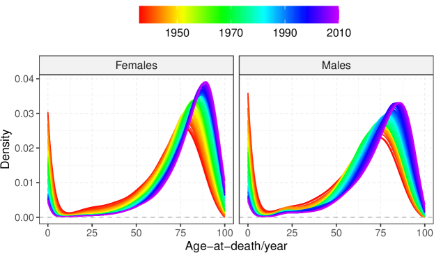
Figure 1: Time-varying densities of age-at-death (in years) for the US from 1936 to 2010.

Recently, there has been intensive interest in comparing distributions with the Wasserstein distance, both in theory and applications (e.g. Bolstad et al., 2003; Bigot et al., 2017; Galichon, 2017; Cazelles et al., 2018; Bigot et al., 2019), and in visualization (e.g. Delicado and Vieu, 2017). In the one-dimensional case that we consider here, it is well known that the Wasserstein transport can also be expressed in terms of quantile functions (Hoeffding, 1940; Zhang and Müller, 2011; Chowdhury and Chaudhuri, 2016).

Our goal is to develop statistical models that reflect instantaneous evolution of such temporal flows of distributions. Starting with the Monge-Kantorovich problem (e.g., Ambrosio, 2003; Villani, 2003, 2008), given two probability measures $p_{1}$ and $p_{2}$, one aims to transport the pile of mass distributed as in $p_{1}$ to that as in $p_{2}$ while minimizing the transport cost. The transport map attaining the minimum transport cost defines the optimal transport from $p_{1}$ to $p_{2}$. Based on such optimal transport maps, basic concepts such as tangent bundles and exponential and logarithmic maps in Riemannian manifolds can be generalized to the space of univariate probability distributions endowed with the Wasserstein distance, which form a quasi-Riemannian manifold (e.g., Ambrosio et al., 2008; Bigot et al., 2017; Zemel and Panaretos, 2019). The log map, defined as the difference between the optimal transport and identity maps, captures the direction and distance of each small element of mass along the order-preserving transport from the starting probability measure to the target measure and can be used to quantify the change between the two probability measures. Hence, we utilize temporal derivatives of log maps, the Wasserstein temporal gradients, to model the instantaneous temporal evolution of distributions. For this purpose, we harness local Fréchet regression (Petersen and Müller, 2019a) to first smooth the observed probability measures over time due to the discrepancy between the true conditional Fréchet mean and the observed distributions and then estimate the Wasserstein temporal gradients by difference quotients based on the local Fréchet regression estimates.

The Wasserstein temporal gradients that we target are introduced in Section 2, with estimation and asymptotic theory in Section 3. In Section 4, we discuss implementation details, followed by a simulation study. Applications are demonstrated in Section 5 for longitudinal household income and human mortality data.

2 Preliminaries

2.1 Optimal Transport in the Wasserstein Space

Given a compact interval $\mathcal{D}$ in $\mathbb{R}$, we focus on the Wasserstein space $\mathcal{W}=\mathcal{W}(\mathcal{D})$ of distributions on $\mathcal{D}$ (for which second moments are finite), endowed with the $\mathcal{L}^{2}$-Wasserstein distance $d_{W}$. This metric is related to the solution of Monge’s optimal transport problem (Villani, 2003) and has repeatedly been rediscovered, with examples including Mallow’s distance (Mallows, 1972), earth mover’s distance (Rubner et al., 1997) or quantile normalization (Bolstad et al., 2003).

Specifically, the $\mathcal{L}^{2}$-Wasserstein distance between any $p_{1},p_{2}\in\mathcal{W}$ is the square root of

$$d^{2}_{W}(p_{1},p_{2})=\inf_{g\#p_{1}=p_{2}}\int_{\mathcal{D}}[x-g(x)]^{2}\ \mathrm{d}p_{1}(x),$$ (1)

where $g\#p$ is a push-forward measure such that $g\#p(A)=p(\{x:g(x)\in A\})$, for any measurable function $g\colon\mathbb{R}\rightarrow\mathbb{R}$, distribution $p\in\mathcal{W}$ and set $A\subseteq\mathbb{R}$. It is well known (e.g., Cambanis et al., 1976) that if $p_{1}$ is atomless, the minimum in (1) is attained at the optimal transport map $\Upsilon_{p_{1},p_{2}}=F^{-1}_{2}\circ F_{1}$ from $p_{1}$ to $p_{2}$, and is $d^{2}_{W}(p_{1},p_{2})=\int_{0}^{1}[F^{-1}_{1}(u)-F^{-1}_{2}(u)]^{2}\ \mathrm{d}u$. Here, $F_{l}$ and $F^{-1}_{l}$ are the cumulative distribution function and quantile function of $p_{l}$ for $l=1,2$, where cumulative distribution functions are considered to be right continuous and quantile functions to be left continuous. A distribution $p$ is atomless if it has a continuous cumulative distribution function.

Basic concepts of Riemannian manifolds can be analogously defined in the Wasserstein space $\mathcal{W}$ based on optimal transport maps (e.g., Ambrosio et al., 2008; Bigot et al., 2017; Zemel and Panaretos, 2019). Suppose that $p_{0}$ is an atomless reference probability measure in $\mathcal{W}$. The tangent space at $p_{0}$ is defined as (Equation (8.5.1), Ambrosio et al., 2008)

$$\mathscr{T}_{p_{0}}={\overline{\{\eta(\Upsilon_{p_{0},p}-{\rm id}):p\in\mathcal{W},\ \eta>0\}}}^{\mathcal{L}^{2}_{p_{0}}},$$

where $\mathcal{L}^{2}_{p_{0}}=\mathcal{L}^{2}_{p_{0}}(\mathcal{D})$ is the Hilbert space of $p_{0}$-square-integrable functions on $\mathcal{D}\subset\mathbb{R}$, with inner product $\langle\cdot,\cdot\rangle_{p_{0}}$ and norm $\|\cdot\|_{p_{0}}$; we reserve the notations without subscripts $\langle\cdot,\cdot\rangle$ and $\|\cdot\|$ for the the inner product and norm corresponding to the Lebesgue measure. Due to the atomlessness of $p_{0}$, the tangent space $\mathscr{T}_{p_{0}}$ is a subspace of $\mathcal{L}^{2}_{p_{0}}$ equipped with the same inner product and induced norm. The exponential map $\mathrm{Exp}_{p_{0}}:\mathscr{T}_{p_{0}}\rightarrow\mathcal{W}$ is then defined by

$$\mathrm{Exp}_{p_{0}}g=(g+{\rm id})\#p_{0},\quad\text{for }g\in\mathscr{T}_{p_{0}}.$$

Although the exponential map here is not a local homeomorphism as in Riemannian manifolds (Ambrosio et al., 2004), any $p\in\mathcal{W}$ can be recovered from $p_{0}$ by $\mathrm{Exp}_{p_{0}}(\Upsilon_{p_{0},p}-{\rm id})$, which motivates the definition of the inverse of the exponential map, i.e., the logarithmic map $\mathrm{Log}_{p_{0}}:\mathcal{W}\rightarrow\mathscr{T}_{p_{0}}$,

$$\mathrm{Log}_{p_{0}}p=\Upsilon_{p_{0},p}-{\rm id},\quad\text{for }p\in\mathcal{W}.$$

The tangent vector given by log maps quantifies the difference between $p_{0}$ and $p$. Indeed, $\|\mathrm{Log}_{p_{0}}p\|_{p_{0}}=d_{W}(p_{0},p)$. Furthermore, the difference between optimal transport maps and the identity map reveals how mass is transported between distributions provided that the order is preserved. Specifically, given $x\in\mathcal{D}$, if $\Upsilon_{p_{1},p_{2}}(x)>x$ (respectively, $\Upsilon_{p_{1},p_{2}}(x)<x$), then $x$ should be moved to the right (respectively, left) to $\Upsilon_{p_{1},p_{2}}(x)$ in order to keep its rank, i.e., $F_{2}(\Upsilon_{p_{1},p_{2}}(x))=F_{1}(x)$.

2.2 Wasserstein Temporal Gradients

Let $(T,P)$ be a pair of random elements in $\mathcal{T}\times\mathcal{W}$ with joint distribution $\mathcal{F}$, where $\mathcal{T}\subseteq\mathbb{R}$ is the time domain. We assume

1. $P$ is atomless almost surely.

Note that $\mathbb{E}[d^{2}_{W}(P,p)\mid T=t]\leq{\rm diam}(\mathcal{D})^{2}<\infty$ for all $p\in\mathcal{W}$ and $t\in\mathcal{T}$. Since the Wasserstein space $\mathcal{W}$ is a Hadamard space (Kloeckner, 2010), there exists a unique minimizer of $\mathbb{E}[d^{2}_{W}(P,\cdot)\mid T=t]$ (Sturm, 2003). Thus, the conditional Fréchet mean $\mu_{\oplus}(t)$ of $P$ given $T=t$ is well-defined; specifically,

$$\mu_{\oplus}(t)=\operatorname*{argmin}_{p\in\mathcal{W}}M(p,t),\quad\text{with }M(p,t)\coloneqq\mathbb{E}[d^{2}_{W}(P,p)\mid T=t],$$

and the quantile function of $\mu_{\oplus}(t)$ is given by $F^{-1}_{\mu_{\oplus}(t)}(\cdot)=\mathbb{E}[F^{-1}_{P}(\cdot)\mid T=t]$, where $F^{-1}_{P}$ is the quantile function of $P$.

To model the instantaneous temporal evolution of probability distributions, we are aiming to generalize the notion of derivatives, which are used to quantify the instantaneous change of differentiable real-valued functions, to the scenario of temporal distribution flows. As discussed in Section 2.1, log maps quantify the discrepancy between two probability distributions. We note that the atomlessness of $\mu_{\oplus}(t)$ is guaranteed by (A1). Hence, a measure of instantaneous temporal evolution of distributions, the Wasserstein temporal gradient at time $t\in\mathcal{T}$ can be defined by

$$V_{t} =\lim_{\Delta\rightarrow 0}\frac{\mathrm{Log}_{\mu_{\oplus}(t)}\mu_{\oplus}(t+\Delta)}{\Delta}$$ (2)

$$=\lim_{\Delta\rightarrow 0}\frac{F^{-1}_{\mu_{\oplus}(t+\Delta)}\circ F_{\mu_{\oplus}(t)}-{\rm id}}{\Delta}$$

$$=\frac{\partial F^{-1}_{\mu_{\oplus}(t)}}{\partial t}\circ F_{\mu_{\oplus}(t)},\quad{\mu_{\oplus}(t)\text{-a.e.}},$$

provided that the bivariate function $(t,u)\mapsto F^{-1}_{\mu_{\oplus}(t)}(u)$ is differentiable with respect to $t$. Here, $F_{\mu_{\oplus}(s)}$ and $F^{-1}_{\mu_{\oplus}(s)}$ are the cumulative distribution function and quantile function of $\mu_{\oplus}(s)$ for $s\in\mathcal{T}$. If there exists $g\in\mathcal{L}^{1}(\mathcal{T})$ such that $d_{W}(\mu_{\oplus}(s),\mu_{\oplus}(t))\leq\int_{s}^{t}g(x)\ \mathrm{d}x$, then $\mu_{\oplus}$ is an absolutely continuous curve in the Wasserstein space, and $V_{t}$ is also referred to as the velocity vector of $\mu_{\oplus}$ (Ambrosio et al., 2004).

Example 1.

For $t\in\mathcal{T}$, let $\mu_{\oplus}(t)=\mathcal{N}_{[0,1]}(\zeta_{t},\upsilon_{t}^{2})$ be a truncated Gaussian distribution on the interval $[0,1]$. Then the Wasserstein temporal gradient at $t$ is

$$V_{t}(x) =\zeta_{t}^{\prime}+(x-\zeta_{t})\frac{\upsilon_{t}^{\prime}}{\upsilon_{t}}$$

$$\quad-\upsilon_{t}\frac{F_{\mu_{\oplus}(t)}(x)\left[\frac{\upsilon_{t}^{\prime}}{\upsilon_{t}}+\left(\frac{\zeta_{t}}{\upsilon_{t}}\right)^{\prime}\right]\varphi\left(\frac{1-\zeta_{t}}{\upsilon_{t}}\right)+(1-F_{\mu_{\oplus}(t)}(x)\left(\frac{\zeta_{t}}{\upsilon_{t}}\right)^{\prime}\varphi\left(\frac{-\zeta_{t}}{\upsilon_{t}}\right)}{\varphi\circ\Phi^{-1}\left(F_{\mu_{\oplus}(t)}(x)\Phi\left(\frac{1-\zeta_{t}}{\upsilon_{t}}\right)+(1-F_{\mu_{\oplus}(t)}(x))\Phi\left(\frac{-\zeta_{t}}{\upsilon_{t}}\right)\right)},$$

where $F_{\mu_{\oplus}(t)}(x)=[\Phi((x-\zeta_{t})/\upsilon_{t})-\Phi(-\zeta_{t}/\upsilon_{t})]/[\Phi((1-\zeta_{t})/\upsilon_{t})-\Phi(-\zeta_{t}/\upsilon_{t})]$, $\Phi$ and $\varphi$ are the cumulative distribution function and density of standard normal distributions, respectively, and we use the notation $g_{t}^{\prime}=(\mathrm{d}/\mathrm{d}t)g_{t}=(\mathrm{d}/\mathrm{d}t)g(t)$ for a function $g$. Densities and Wasserstein temporal gradients of $\mathcal{N}_{[0,1]}(\zeta_{t},\upsilon_{t}^{2})$ with different values of $\zeta_{t}$ and $\upsilon_{t}$ are shown in Figure 2.

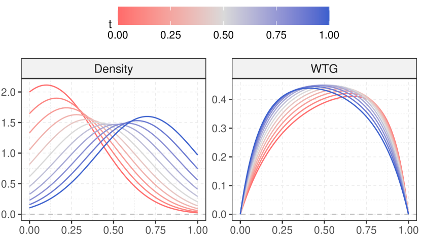
(a) $\zeta_{t}=0.1+0.6t$, $\upsilon_{t}\equiv 0.3$.

(b) $\zeta_{t}=0.1+0.8(t-0.5)^{2}$, $\upsilon_{t}=0.3-0.1t$.

Figure 2: Densities and Wasserstein temporal gradients of $\mu_{\oplus}(t)=\mathcal{N}_{[0,1]}(\zeta_{t},\upsilon_{t}^{2})$, for $t\in[0,1]$.

Example 2.

For $t\in\mathcal{T}$, let $\mu_{\oplus}(t)$ be atomless distributions in a location-scale family with location and scale parameters being $\xi_{t}$ and $\varsigma_{t}$, respectively. Specifically, the cumulative distribution function of $\mu_{\oplus}(t)$ is given by $x\mapsto G((x-\xi_{t})/\varsigma_{t})$, where $G\colon\mathbb{R}\rightarrow[0,1]$ is a template cumulative distribution function. Then the Wasserstein temporal gradient at $t\in\mathcal{T}$ is

$$V_{t}(x)=\xi_{t}^{\prime}+(x-\xi_{t})\frac{\varsigma_{t}^{\prime}}{\varsigma_{t}}.$$

For a real-valued differentiable function $g:\mathcal{T}\rightarrow\mathbb{R}$,

$$\frac{\ \mathrm{d}F_{\mu_{\oplus}(t)}(g(t))}{\ \mathrm{d}t}=0\quad\text{if and only if}\quad g^{\prime}(t)=V_{t}(g(t)).$$

Thus, comparing the actual flow $g^{\prime}(t)$ for a given longitudinal trajectory $g(t)$ with the optimal flow $V_{t}(g(t))$ provides insights into how the rank of $g(t)$ changes at each time $t$. If $g^{\prime}(t)>V_{t}(g(t))$ (respectively, $g^{\prime}(t)<V_{t}(g(t))$), then $\frac{\ \mathrm{d}}{\ \mathrm{d}t}F_{\mu_{\oplus}(t)}(g(t))$ is positive (respectively, negative), i.e., the rank of $g(t)$ increases (respectively, decreases) instantaneously at time $t$.

3 Estimation and Theory

3.1 Distribution Estimation

In practice, distributions are usually not fully observed. This creates an additional challenge for the implementation of the Wasserstein temporal gradients. This issue can be addressed, for example, by estimating cumulative distribution functions (e.g., Aggarwal, 1955; Read, 1972; Falk, 1983; Leblanc, 2012), or estimating quantile functions (e.g., Parzen, 1979; Falk, 1984; Yang, 1985; Cheng and Parzen, 1997) of the underlying distributions from which the observed data are sampled. Note that with any quantile function estimator $\widehat{F}^{-1}$ (respectively, cumulative distribution function estimator $\widehat{F}$), the corresponding cumulative distribution function (respectively, quantile function) can be obtained by right (respectively, left) continuous inversion,

$$\widehat{F}(x)=\sup\{u\in[0,1]:\widehat{F}^{-1}(u)\leq x\},\quad\text{for }x\in\mathbb{R},$$

$$\quad\quad\quad\quad\text{ respectively, }\widehat{F}^{-1}(u)=\inf\{x\in\mathcal{D}:\widehat{F}(x)\geq u\},\quad\text{for }u\in(0,1).$$

Alternatively, one can first estimate densities (Panaretos and Zemel, 2016; Petersen and Müller, 2016) and then obtain the cumulative distribution functions and quantile functions by integration and inversion.

Suppose $\{(T_{i},P_{i})\}_{i=1}^{n}$ are $n$ independent realizations of $(T,P)$. Available observations are samples of independent measurements $\{X_{ij}\}_{j=1}^{m_{i}}$ generated from $P_{i}$, respectively, where $m_{i}$ are the sample sizes which may vary across distributions $P_{i}$, for $i=1,\ldots,n$. Note that the observed data $X_{ij}$ result from two independent random mechanisms: The first of these generates independently and identically distributed pairs $(T_{i},P_{i})$; the second generates samples of observations $\{X_{ij}\}_{j=1}^{m_{i}}$ according to each distribution $P_{i}$, i.e., $X_{ij}\sim P_{i}$ independently.

For a given distribution $p\in\mathcal{W}$, with a cumulative distribution function estimate $\widehat{F}$ obtained by any estimation method based on a random sample generated from $p$, we denote by $\widehat{p}=\pi(\widehat{F})$ the distribution associated with $\widehat{F}$. We make the following assumption on the discrepancy of the estimated and true probability distributions for the theoretical analysis of the Wasserstein temporal gradient estimation.

1. For any distribution $p\in\mathcal{W}$, with nonnegative decreasing sequence $\alpha_{m}=o(1)$ as $m\rightarrow\infty$, the corresponding estimate $\widehat{p}$ based on a sample of size $m$ generated from $p$ satisfies

   $$\begin{gathered}\sup_{p\in\mathcal{W}}\mathbb{E}[d^{2}_{W}(\widehat{p},p)]=O(\alpha_{m}).\end{gathered}$$

We note that this assumption can be easily satisfied. For example, the density estimator proposed by Panaretos and Zemel (2016) satisfies (D1) with $\alpha_{m}=m^{-1/2}$. If only considering the distributions in $\mathcal{W}$ with densities satisfying

$$\begin{gathered}\sup_{x\in{\mathrm{supp}(f_{p})}}\max\{f_{p}(x),1/f_{p}(x),|f_{p}^{\prime}(x)|\}\leq C,\text{ uniform across }p,\end{gathered}$$

where $f_{p}$ is the density function of a distribution $p\in\mathcal{W}$, $\mathrm{supp}(f_{p})=\mathcal{D}$ is the support of $p$ and $C>0$ is a constant, then the empirical measure satisfies (D1) with $\alpha_{m}=m^{-1}$.

In order to deal with the estimation of $n$ distributions simultaneously, we also require

1. There exists a sequence $m=m(n)$ such that $\min_{1\leq i\leq n}\{m_{i}\}\geq m$ and $m\rightarrow\infty$ as $n\rightarrow\infty$.

3.2 Estimation of Wasserstein Temporal Gradients

We assume that for each $i=1,\ldots,n$, we obtain an estimate $\widehat{F}_{P_{i}}$ of the cumulative distribution function of $P_{i}$ by one of the methods discussed in Section 3.1 from the observed data $\{X_{ij}\}_{j=1}^{m_{i}}$. Denote by $\widehat{P}_{i}=\pi(\widehat{F}_{P_{i}})$ the distribution associated with $\widehat{F}_{P_{i}}$. Since the discrepancy $\mathbb{E}[d^{2}_{W}(P_{i},\mu_{\oplus}(T_{i}))\mid T_{i}]$ between the random distributions $P_{i}$ and the conditional Fréchet means $\mu_{\oplus}(T_{i})$ does not vanish as $n\rightarrow\infty$, difference quotients based on the estimated distributions $\widehat{P}_{i}$ are not directly suitable as an estimate of Wasserstein temporal gradients.

Accordingly, we utilize local Fréchet regression (Petersen and Müller, 2019a) to smooth the distributions $\{\widehat{P}_{i}\}$ over time, which yields consistent estimates of $\mu_{\oplus}(t)$, for any $t\in\mathcal{T}$. Following Petersen and Müller (2019a), we define the localized Fréchet mean by

$$\nu_{\oplus}(t)=\operatorname*{argmin}_{p\in\mathcal{W}}L_{h}(p,t),\quad\text{with }L_{h}(p,t)=\mathbb{E}[w(T,t,h)d^{2}_{W}(P,p)].$$ (3)

Here, $w(s,t,h)=K_{h}(s-t)[\kappa_{2}(t)-\kappa_{1}(t)(s-t)]/\sigma_{0}^{2}(t)$, where $\kappa_{z}(t)=\mathbb{E}[K_{h}(T-t)(T-t)^{z}]$, for $z=0,1,2$, $\sigma_{0}^{2}(t)=\kappa_{0}(t)\kappa_{2}(t)-\kappa_{1}(t)^{2}$, $K_{h}(\cdot)=K(\cdot/h)/h$, $K$ is a smoothing kernel, i.e., a density function symmetric around zero, and $h=h(n)>0$ is a bandwidth sequence. If assuming the distributions $P_{i}$ are fully observed, setting $\widehat{w}(s,t,h)=K_{h}(s-t)[\widehat{\kappa}_{2}(t)-\widehat{\kappa}_{1}(t)(s-t)]/\widehat{\sigma}_{0}^{2}(t)$, where $\widehat{\kappa}_{z}(t)={n}^{-1}\sum_{i=1}^{n}K_{h}(T_{i}-t)(T_{i}-t)^{z}$, for $z=0,1,2$, and $\widehat{\sigma}_{0}^{2}(t)=\widehat{\kappa}_{0}(t)\widehat{\kappa}_{2}(t)-\widehat{\kappa}_{1}(t)^{2}$, an oracle local Fréchet regression estimate is

$$\widetilde{\nu}_{\oplus}(t)=\operatorname*{argmin}_{p\in\mathcal{W}}\widetilde{L}_{n}(p,t),\quad\text{with }\widetilde{L}_{n}(p,t)={n}^{-1}\sum_{i=1}^{n}\widehat{w}(T_{i},t,h)d^{2}_{W}(P_{i},p).$$ (4)

In practice, we usually only observe random samples of measurements $X_{ij}$ generated from $P_{i}$. Replacing $P_{i}$ with the corresponding estimates $\widehat{P}_{i}$ as discussed in Section 3.1, a data-based local Fréchet regression estimate is

$$\widehat{\nu}_{\oplus}(t)=\operatorname*{argmin}_{p\in\mathcal{W}}\widehat{L}_{n}(p,t),\quad\text{with }\widehat{L}_{n}(p,t)={n}^{-1}\sum_{i=1}^{n}\widehat{w}(T_{i},t,h)d^{2}_{W}(\widehat{P}_{i},p).$$ (5)

For simplicity, we assume for theoretical analysis that the support of the marginal density $f_{T}$ of $T$, i.e., $\mathcal{T}=\{t\in\mathbb{R}:f_{T}(t)>0\}$, is connected. Let $\mathcal{T}^{\circ}$ be the interior of $\mathcal{T}$. Furthermore, we require the following assumptions for the asymptotic analysis of the weights $w(T,t,h)$ and $\widehat{w}(T_{i},t,h)$ in $\nu_{\oplus}(t)$ and $\widehat{\nu}_{\oplus}(t)$, respectively.

1. The kernel $K$ is a probability density function, symmetric around zero and continuous on $[-1,1]$, such that $K(x)=0$, for all $|x|>1$.

2. The marginal density $f_{T}$ of $T$ exists and is continuous on $\mathcal{T}$ and twice continuously differentiable on $\mathcal{T}^{\circ}$. The second-order derivative $f_{T}^{\prime\prime}$ is bounded, $\sup_{t\in\mathcal{T}^{\circ}}|f_{T}^{\prime\prime}(t)|<\infty$.

For any $t\in\mathcal{T}^{\circ}$, with the local Fréchet regression estimate $\widehat{\nu}_{\oplus}(t)$ as per (5) and some small $\Delta>0$, an estimate of the Wasserstein temporal gradient $V_{t}$ in (2) is then given by

$$\begin{gathered}\widehat{V}_{t,\Delta}=\frac{F^{-1}_{\widehat{\nu}_{\oplus}(t+\Delta)}\circ F_{\widehat{\nu}_{\oplus}(t)}-{\rm id}}{\Delta},\end{gathered}$$ (6)

where $F_{\widehat{\nu}_{\oplus}(s)}$ and $F^{-1}_{\widehat{\nu}_{\oplus}(s)}$ are the cumulative distribution function and quantile function of $\widehat{\nu}_{\oplus}(s)$ for $s\in\mathcal{T}$.

3.3 Parallel Transport

Note that the true and estimated Wasserstein temporal gradients lie in different tangent spaces; specifically, $V_{t}\in\mathscr{T}_{\mu_{\oplus}(t)}$ and $\widehat{V}_{t,\Delta}\in\mathscr{T}_{\widehat{\nu}_{\oplus}(t)}$. To quantify the estimation discrepancy of $\widehat{V}_{t,\Delta}$, an expedient tool is parallel transport, which is commonly used for manifold-valued data (e.g., Yuan et al., 2012; Lin and Yao, 2018; Petersen and Müller, 2019b; Chen et al., 2020). For two probability measures $p_{1},p_{2}\in\mathcal{W}$, a parallel transport operator $\Gamma_{p_{1},p_{2}}\colon\mathcal{L}^{2}_{p_{1}}\rightarrow\mathcal{L}^{2}_{p_{2}}$ is defined by

$$\Gamma_{p_{1},p_{2}}g=g\circ F^{-1}_{1}\circ F_{2},\quad\text{for }g\in\mathcal{L}^{2}_{p_{1}},$$

where $F_{2}$ and $F^{-1}_{1}$ are the cumulative distribution function of $p_{2}$ and quantile function of $p_{1}$, respectively.

Note that since $p_{1}$ and $p_{2}$ are atomless, the tangent spaces satisfy $\mathscr{T}_{p_{k}}\subset\mathcal{L}^{2}_{p_{k}}$ for $k=1,2$, and the parallel transport operator $\Gamma_{p_{1},p_{2}}|_{\mathscr{T}_{p_{1}}}$ restricted to the tangent space $\mathscr{T}_{p_{1}}$ defines the parallel transport between tangent spaces $\mathscr{T}_{p_{1}}$ and $\mathscr{T}_{p_{2}}$. Furthermore, the parallel transport operator $\Gamma_{p_{2},p_{1}}$ from $\mathcal{L}^{2}_{p_{2}}$ to $\mathcal{L}^{2}_{p_{1}}$ is the adjoint operator of $\Gamma_{p_{1},p_{2}}$, i.e., $\langle\Gamma_{p_{1},p_{2}}g_{1},g_{2}\rangle_{p_{2}}=\langle g_{1},\Gamma_{p_{2},p_{1}}g_{2}\rangle_{p_{1}}$. Thus, the discrepancy between functions $g_{1}\in\mathscr{T}_{p_{1}}$ and $g_{2}\in\mathscr{T}_{p_{2}}$ can be quantified by $\|\Gamma_{p_{2},p_{1}}g_{2}-g_{1}\|_{p_{1}}$.

3.4 Asymptotic Theory

As discussed in Section 3.3, in order to justify $\|\Gamma_{\widehat{\nu}_{\oplus}(t),\mu_{\oplus}(t)}\widehat{V}_{t,\Delta}-V_{t}\|_{\mu_{\oplus}(t)}$ as a measure of estimation discrepancy of $\widehat{V}_{t,\Delta}$, we require the atomlessness of $\mu_{\oplus}(t)$ and $\widehat{\nu}_{\oplus}(t)$. The former follows from (A1). However, the latter is not guaranteed in general. For theoretical derivations, we instead consider an atomless variant $\widecheck{\nu}_{\oplus}(t)$ of $\widehat{\nu}_{\oplus}(t)$, which is defined as follows. Suppose $\min\mathcal{D}=x_{0}<x_{1}<\dots<x_{B}=\max\mathcal{D}$ is an equidistant grid on $\mathcal{D}$ with increment $b$. Then the cumulative distribution function of $\widecheck{\nu}_{\oplus}(t)$ is given by $F_{\widecheck{\nu}_{\oplus}(t)}(x)=F_{\widehat{\nu}_{\oplus}(t)}(x_{l-1})+b^{-1}(x-x_{l-1})[F_{\widehat{\nu}_{\oplus}(t)}(x_{l})-F_{\widehat{\nu}_{\oplus}(t)}(x_{l-1})]$, for $x\in[x_{l-1},x_{l})$; $F_{\widecheck{\nu}_{\oplus}(t)}(x)=0$ and 1 for $x<x_{0}$ and $x\geq x_{B}$, respectively. We assume that $b=b(n)$ is a positive sequence such that $b\rightarrow 0$ as $n\rightarrow\infty$. Hence, an estimate of the Wasserstein temporal gradient at time $t$ based on $\widecheck{\nu}_{\oplus}(s)$ with $s\in\mathcal{T}$ is given by

$$\begin{gathered}\widecheck{V}_{t,\Delta}=\frac{F^{-1}_{\widecheck{\nu}_{\oplus}(t+\Delta)}\circ F_{\widecheck{\nu}_{\oplus}(t)}-{\rm id}}{\Delta}.\end{gathered}$$

To obtain the convergence rate of $\widecheck{V}_{t,\Delta}$, we also require the following assumption.

1. The bivariate function $(t,u)\mapsto F^{-1}_{\mu_{\oplus}(t)}(u)$ is twice differentiable and $(t,u)\mapsto\partial^{2}F^{-1}_{\mu_{\oplus}(t)}(u)/(\partial t\partial u)$ is continuous with respect to $u$. There exists a constant $C>0$ such that $\sup_{x\in\mathcal{D}}f_{\mu_{\oplus}(t)}(x)\leq C$, $\int_{0}^{1}\sup_{t\in\mathcal{T}}|\partial^{2}F^{-1}_{\mu_{\oplus}(t)}(u)/\partial t^{2}|^{2}\ \mathrm{d}u\leq C$, and $\sup_{t\in\mathcal{T},\,u\in(0,1)}|\partial^{2}F^{-1}_{\mu_{\oplus}(t)}(u)/(\partial t\partial u)|\leq C$.

We take $\Delta=h$; this choice, together with suitable values for $h$, $b$ and $\Delta$, will lead to Wasserstein temporal gradient estimates $\widecheck{V}_{t,\Delta}$ with an asymptotic rate of convergence that matches the well-known optimal rate of derivative estimation for nonparametric regression for the case of real-valued responses assuming twice continuous differentiability of the regression function. This optimal rate is for example achieved by derivative estimates based on local polynomial fitting (Müller, 1987; Fan and Gijbels, 1996).

Theorem 1.

Assume (A1)–(A2), (D1)–(D2) and (R1)–(R2). With $\Delta=h$, if $h\rightarrow 0$, $nh^{3}\rightarrow\infty$, $bh^{-1}\rightarrow\infty$, and $\alpha_{m}h^{-1}\rightarrow 0$,

$$\left\|\Gamma_{\widecheck{\nu}_{\oplus}(t),\mu_{\oplus}(t)}\widecheck{V}_{t,\Delta}-V_{t}\right\|_{\mu_{\oplus}(t)}$$

$$\quad=\left\|\frac{F^{-1}_{\widecheck{\nu}_{\oplus}(t+h)}-F^{-1}_{\widecheck{\nu}_{\oplus}(t)}}{h}-\frac{\partial F^{-1}_{\mu_{\oplus}(t)}}{\partial t}\right\|$$

$$\quad=O\left({h}\right)+O_{p}\left((nh^{3})^{-1/2}\right)+O\left(bh^{-1}\right)+O_{p}\left((\alpha_{m}h^{-1})^{1/2}\right).$$

Furthermore, with $h\sim n^{-1/{5}}$, $b=O(n^{-{2/5}})$ and $\alpha_{m}=O(n^{-{3/5}})$,

$$\left\|\Gamma_{\widecheck{\nu}_{\oplus}(t),\mu_{\oplus}(t)}\widecheck{V}_{t,\Delta}-V_{t}\right\|_{\mu_{\oplus}(t)}=O_{p}\left(n^{-{1/5}}\right).$$ (7)

Proofs are in the appendix.

4 Implementation and Simulations

There are two tuning parameters for implementation of Wasserstein temporal gradients, namely the bandwidth $h$ involved in the local Fréchet regression as per (5) and the time increment $\Delta$ used in the difference quotient estimator as per (6). As suggested by the theoretical analysis in Section 3.4, we take $\Delta=h$ in practice. We choose the bandwidth $h$ by leave-one-out cross validation, where the objective function to be minimized is the mean discrepancy between the local Fréchet regression estimates and the observed distributions; specifically,

$$h=\operatorname*{argmin}_{h^{\prime}}n^{-1}\sum_{i=1}^{n}d^{2}_{W}(\widehat{\nu}_{\oplus h^{\prime}}^{-i}(T_{i}),\widehat{P}_{i}),$$

where $\widehat{\nu}_{\oplus h^{\prime}}^{-i}(T_{i})$ is the local Fréchet regression estimate of $\mu_{\oplus}(T_{i})$ obtained with bandwidth $h^{\prime}$ based on the sample excluding the $i$th pair $(T_{i},\widehat{P}_{i})$, i.e.,

$$\widehat{\nu}_{\oplus h^{\prime}}^{-i}(T_{i})=\operatorname*{argmin}_{p\in\mathcal{W}}\frac{1}{n-1}\sum_{i^{\prime}\neq i}\widehat{w}(T_{i^{\prime}},T_{i},h^{\prime})d^{2}_{W}(\widehat{P}_{i^{\prime}},p),$$

and $\widehat{P}_{i}$ is the estimate of $P_{i}$ based on the observed measurements $\{X_{ij}\}_{j=1}^{m_{i}}$ as discussed in Section 3.1. In practice, we replace leave-one-out cross validation by 10-fold cross validation when $n>30$.

We generated data for simulations as follows:

1. Set $\mu_{\oplus}(t)=\mathcal{N}_{[0,1]}(\zeta_{t},\upsilon_{t}^{2})$, a truncated Gaussian distribution on $[0,1]$ with $\zeta_{t}=(t-0.2)(t-0.5)(t-0.9)+0.2$ and $\upsilon_{t}=0.15+0.03\sin(2\pi t)$.

2. Sample $a_{i}\sim\mathrm{Unif}\{\pm 10\pi,\pm 11\pi,\ldots,\pm 14\pi\}$ and $T_{i}\sim\mathrm{Unif}[0,1]$ independently, for $i=1,\ldots,n$. Set $P_{i}=g_{a_{i}}\#\mu_{\oplus}(T_{i})$, where $g_{a}(x)=x-|a|^{-1}\sin(ax)$ with $a\in\mathbb{R}\backslash\{0\}$ and $x\in\mathbb{R}$.

3. Draw an independently and identically distributed sample $\{X_{ij}\}_{j=1}^{m}$ of size $m$ from each of the distributions $\{P_{i}\}_{i=1}^{n}$.

Four cases were considered with $n\in\{50,200\}$ and $m\in\{25,500\}$. We simulated 500 runs for each pair $(n,m)$. To evaluate the performance of the Wasserstein temporal gradient estimate based on the local Fréchet regression as per (6), we computed the integrated error (IE) for given $t\in[0,1]$; specifically,

$$\begin{gathered}\mathrm{IE}(n,m,t)=\left\|\frac{F^{-1}_{\widehat{\nu}_{\oplus}(t+\Delta)}-F^{-1}_{\widehat{\nu}_{\oplus}(t)}}{\Delta}-\frac{\partial}{\partial t}F^{-1}_{\mu_{\oplus}(t)}\right\|.\end{gathered}$$ (8)

The results are summarized in the boxplots of IEs in Figure 3. It can be seen that the estimation error decreases as $n$ or $m$ increases.

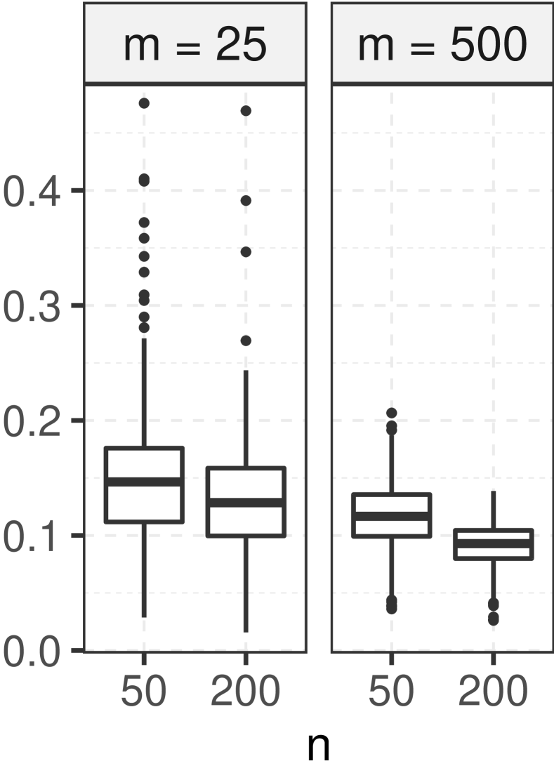
(a) $t=0.25$.

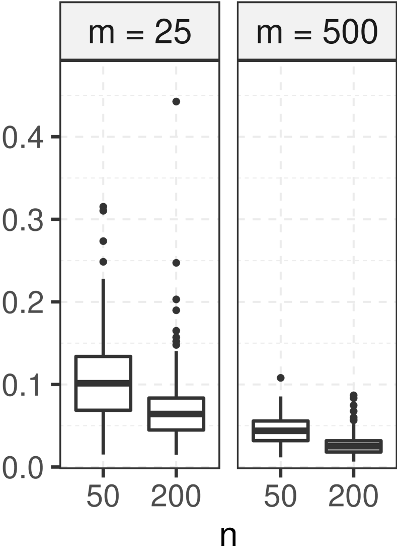
(b) $t=0.5$.

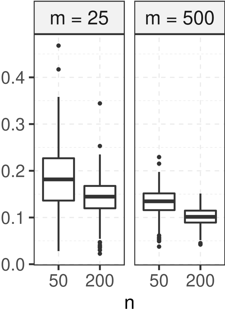
(c) $t=0.75$.

Figure 3: Boxplots of the integrated errors (IEs) as per (8) of the 500 runs for $t\in\{0.25,0.5,0.75\}$ and each $(n,m)$.

5 Applications

In this section, we will demonstrate the proposed Wasserstein gradients for time-dependent household income and human mortality data. As mentioned before, the underlying densities are practically never known and need to be estimated from data that they generate. In the household income and mortality examples, the data are reported in the form of histograms, respectively life tables. Our methods can be applied in a straightforward way to histogram data; specifically we estimate the densities by applying a smoothing step, e.g., using local linear regression. For local Fréchet regression, we use the Epanechnikov kernel function $K(t)=0.75(1-t^{2})\mathbf{1}_{[-1,1]}(t)$ and choose smoothing bandwidths $h$ by cross validation.

5.1 Household Income Data

Many studies have been conducted on income distribution and inequality (Jones, 1997; Heathcote et al., 2010), since this is a major measure of economic equality/inequality. The evolution of income distributions over time is of particular interest as it provides quantification of the directions in which income inequality is evolving. The US Census Bureau provides histogram data of US household income over calendar years from 1994 to 2016, available at https://census.gov. To make incomes of different years comparable, adjustments for inflation have been made, using the year 2000 as baseline for constant dollars.

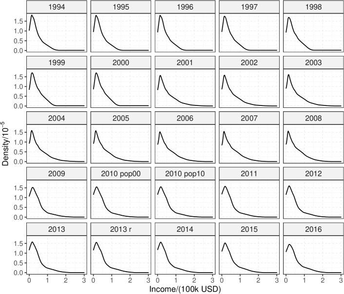
Figure 4: Densities of US household incomes for 1994–2016, where “2010 pop00” and “2010 pop10” represent the distribution of 2010 based on the population census of 2000 and 2010, respectively, and “2013” and “2013 r” represent the distributions on previous and redesigned questionnaires, respectively.

We focus on incomes less than $$300,000$. The data require some preprocessing, as the width of the histogram bins changed between 2000 and 2001; for 2010, due to census changes, two datasets are available based on both census 2010 and 2000 populations; for 2013, two sets of data are also available and one of them is based on a redesigned questionnaire which has been used since then. To mitigate against these changes, which potentially introduce artificial variation, we divided the whole period into four parts: 1994–2000, 2001–2010, 2010–2013 and 2013–2016. Although another change of bin width occurred between 2008 and 2009, we keep the entire period 2001–2010 in order to cover the financial crisis of 2008 well within the time interval. The densities constructed by smoothing the histogram data are shown in Figure 4, where “2010 pop00”, “2010 pop10”, “2013” and “2013 r” represents the income distribution of 2010 based on the population census of 2000 and 2010, and of 2013 based the previous and redesigned questionnaires, respectively.

Figure 4 reveals not much variation in the income distributions over time except around 2008. The estimated Wasserstein temporal gradients as per (6) (with bandwidths $h=1.99$, 1.55, 1.50 and 1.50 years for the four periods, respectively, chosen by cross validation, see Section 4 and time increment $\Delta=h$) demonstrate how the income of poor, middle-class and rich households evolved for the four periods in Figure 5. The Wasserstein temporal gradients for the ending years of each period cannot be well estimated due to the relative large value of $\Delta$, and hence the results for 2000, “2010 pop00”, “2013” and 2016 are not displayed. Since the local Fréchet regression has increased variance near endpoints, the estimated Wasserstein temporal gradients on the two ends of each period are somewhat unreliable.

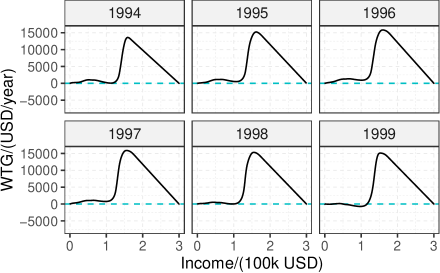
(a) 1994–1999.

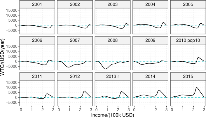
(b) 2001–2015.

Figure 5: Estimates of the Wasserstein temporal gradients (solid curves) as per (6) for US household income distribution flows for 1994–1999 and 2001–2015. Positive values indicate an increasing trend; negative values indicate a decreasing trend.

It can be seen in Figure 5 that for the period 1994–1999, incomes of households at the same percentile levels increased almost throughout, except for relatively poor households whose incomes tended to decrease in 1999. Incomes of households earning more than $150,000 per year increased much faster than the other incomes. For the second period 2001–2010, the economic status of the lower and middle earners was stable in the first three years, rose in 2004–2006, and then declined starting in 2007. Higher incomes declined until 2002, and beginning in 2003, a divide manifested itself in the higher income levels: The lower tier of higher incomes was associated with declining income, whereas the higher tier was associated with increasing income, except for 2007 and 2008. Note that in 2007 and 2008, all household incomes tended to decrease, coinciding with the financial crisis. For the last two periods, it can be seen that household incomes gradually recovered from the crisis. While top incomes above 240,000 US dollars always gained, households with relatively low incomes did not recover until around 2014.

5.2 Human Mortality Data

The analysis of mortality data across countries and species has found interest in demography and statistics (Carey et al., 1992; Chiou and Müller, 2009; Ouellette and Bourbeau, 2011; Hyndman et al., 2013; Shang and Hyndman, 2017). Of particular interest is how the distribution of age-of-death evolves over time. The Human Mortality Database (http://www.mortality.org) provides data of yearly life tables for 37 countries, from which the distributions of ages-at-death in terms of histograms can be extracted.

We focus on ages-at-death in the age interval $[0,100]$ (in years) and take Russia, Sweden and the United States as three examples. The densities obtained by smoothing the histogram data for females and males separately are shown in Figures 6, 7 and 1, respectively. It can been seen that densities of mortality and their changes vary across these three countries, which is partly due to the different domains in terms of calendar years during which country-specific mortality has been recorded, which goes much further into the past for Sweden than for the other countries. Estimates of the Wasserstein temporal gradients have been obtained with bandwidths $h$ chosen by cross validation as discussed in Section 4 per gender and country (see Table 1 for details) and $\Delta=h$.

Table 1: Bandwidths used in the local Fréchet regression for the age-at-death distributions.

	Russia	Sweden	USA
Females	1.87	2.09	2.40
Males	1.66	1.78	2.52

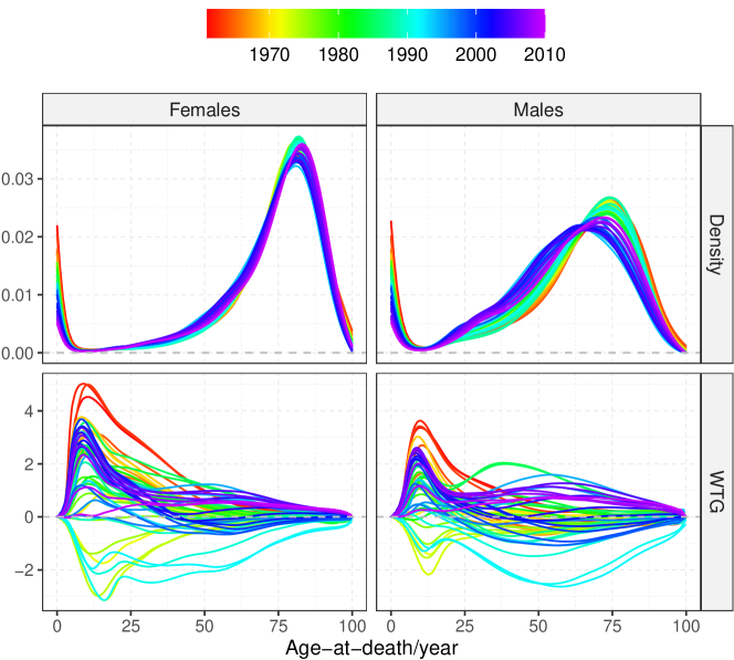
Figure 6: Top: Time-varying densities of age-at-death (in years) with females in the left column and males in the right column for Russia from 1961 to 2010. Bottom: Estimates of the (unit-free) Wasserstein temporal gradients of the age-at-death (in years) distributions from 1961 to 2010, where positive values indicate increasing trend and negative values indicate decreasing trend.

For Russia, the densities of ages-at-death from 1961 to 2010 are shown in the top two panels in Figure 6. The age-at-death distributions are quite different between females and males; female adults tend to live longer than males. The estimates of the Wasserstein temporal gradients for 1961–2010 for Russia are shown in the bottom two panels in Figure 6, and were obtained based on data from 1959 to 2014; the estimated gradients for the first and last two years were excluded due to boundary effects. Between 1970 and 2000, the movement of mortality to higher ages and thus longer life was interrupted, with a lot of variation during this period, and resumed only in the 2000s, where substantial improvement occurs in children’s mortality. In the 1990s, there was a remarkable reversal in the trend of longevity increase, as the estimates of the Wasserstein temporal gradients were negative for those years, especially for young females and mid-age males.

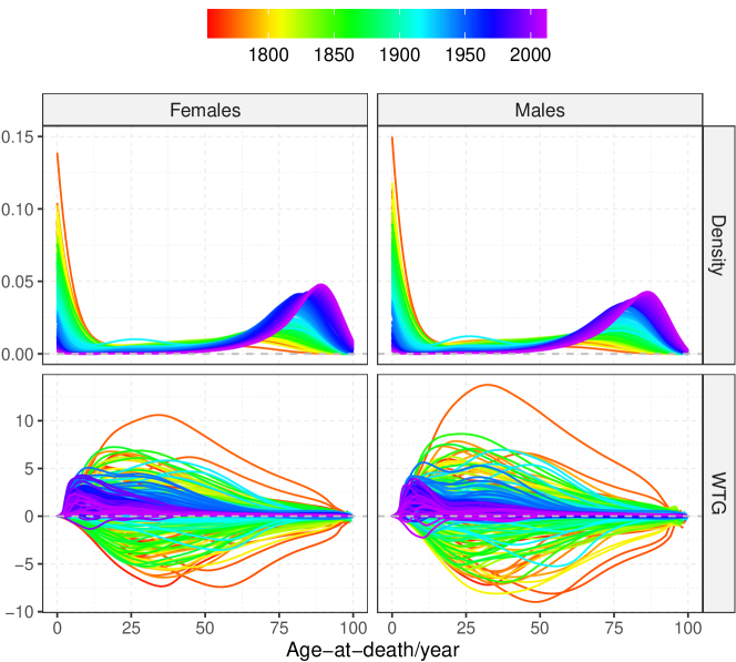
Figure 7: Top: Time-varying densities of age-at-death (in years) with females in the left column and males in the right column for Sweden from 1754 to 2012. Bottom: Estimates of the (unit-free) Wasserstein temporal gradients for the distributions of age-at-death (in years) distributions from 1754 to 2012, where positive values indicate increasing trend; negative values indicate decreasing trend.

For Sweden, as shown in Figure 7, the densities of ages-at-death of females and males are quite similar, indicating a general increase in longevity over the years. The estimated Wasserstein temporal gradients for Sweden in Figure 7 from 1754 to 2012, which are obtained based on data from 1751 to 2016, show some volatility in the age-at-death distributions for both females and males, especially before 1950. Compared to Russia, the evolution of the age-at-death distributions in Sweden is more balanced—years where the distribution moves to the left (right) are followed by years with a rightward (leftward) movement in the distribution. The Wasserstein temporal gradients for Sweden vary in a much larger range than Russia, which is partly due to the inclusion of early calendar years, where the variation of mortality from year to year was much larger, compared to more recent calendar years. For example, the top orange curve for 1773 demonstrates a massive increasing trend in life span for both females and males while the bottom orange curves for 1770–1771 demonstrate a strongly decreasing trend.

For the US, the age-at-death distributions are somewhat similar across genders. The estimates of the Wasserstein temporal gradients from 1936 to 2010 obtained based on data from 1933 to 2015 for the US in Figure 8 indicate that age-at-death distributions tend to move to the right in almost all years, suggesting increasing longevity. However, for several of the years since the 1980s, reversals can be found for both females and males. A major reversal can be found for the males from young adults to middle age during 1983–1987. This puzzling reversal has been attributed to drug use (e.g., Case and Deaton, 2015).

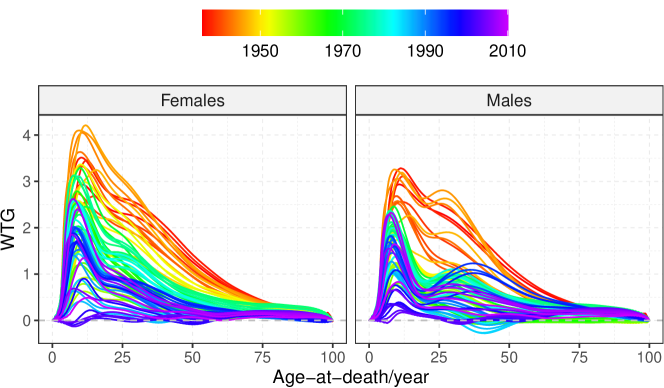
Figure 8: Estimates of the (unit-free) Wasserstein temporal gradients of the age-at-death (in years) distributions for the US from 1936 to 2010, with females on the left and males on the right. Positive values indicate increasing trend; negative values indicate decreasing trend.

Appendix Appendix: Derivation of Theorem 1

For $t\in\mathcal{T}$, we define

$$q_{t}(\cdot) =\mathbb{E}\left[w(T,t,h)F^{-1}_{P}(\cdot)\right],$$

$$\overline{q}_{t}(\cdot) =n^{-1}\sum_{i=1}^{n}w(T_{i},t,h)F^{-1}_{P_{i}}(\cdot),$$

$$\widetilde{q}_{t}(\cdot) =n^{-1}\sum_{i=1}^{n}\widehat{w}(T_{i},t,h)F^{-1}_{P_{i}}(\cdot),$$

$$\widehat{q}_{t}(\cdot) =n^{-1}\sum_{i=1}^{n}\widehat{w}(T_{i},t,h)\widehat{F}^{-1}_{P_{i}}(\cdot),$$

where $F^{-1}_{P}$, $F^{-1}_{P_{i}}$ and $\widehat{F}^{-1}_{P_{i}}$ are the quantile functions of $P$, $P_{i}$ and $\widehat{P}_{i}$, respectively. Considering any fixed $t\in\mathcal{T}^{\circ}$, we will show that

$$\left\|\frac{q_{t+h}-q_{t}}{h}-\frac{\partial F^{-1}_{\mu_{\oplus}(t)}}{\partial t}\right\|=O(h).$$ (A.1)

For $q_{t}$, we will show that with sufficiently small $h$,

$$\partial q_{t}(u)/\partial u>0,\quad\text{for all }u\in(0,1),$$ (A.2)

i.e., $q_{t}$ is a quantile function, whence we will show that

$$\left\|F^{-1}_{\widehat{\nu}_{\oplus}(t)}-q_{t}\right\|\leq\left\|\widehat{q}_{t}-q_{t}\right\|.$$ (A.3)

Hence,

$$\left\|\frac{F^{-1}_{\widehat{\nu}_{\oplus}(t+h)}-F^{-1}_{\widehat{\nu}_{\oplus}(t)}}{h}-\frac{q_{t+h}-q_{t}}{h}\right\|$$

$$\quad\leq h^{-1}\left(\left\|F^{-1}_{\widehat{\nu}_{\oplus}(t+h)}-q_{t+h}\right\|+\left\|F^{-1}_{\widehat{\nu}_{\oplus}(t)}-q_{t}\right\|\right)$$

$$\quad\leq h^{-1}\left(\left\|\widehat{q}_{t+h}-q_{t+h}\right\|+\left\|\widehat{q}_{t}-q_{t}\right\|\right).$$

Furthermore, we will show that

$$\left\|\widehat{q}_{t+h}-\widetilde{q}_{t+h}\right\| =O_{p}\left((\alpha_{m}h)^{1/2}\right),$$ (A.4)

$$\left\|\widetilde{q}_{t+h}-\overline{q}_{t+h}\right\| =O_{p}\left((nh)^{-1/2}\right),$$

$$\left\|\overline{q}_{t+h}-q_{t+h}\right\| =O_{p}\left((nh)^{-1/2}\right).$$

Similar results hold when replacing $t+h$ with $t-h$. We note that for all $t\in\mathcal{T}$, $\|F^{-1}_{\widecheck{\nu}_{\oplus}(t)}-F^{-1}_{\widehat{\nu}_{\oplus}(t)}\|\leq b$, a.s. In conjunction with the atomlessness of $\mu_{\oplus}(t)$ and $\widecheck{\nu}_{\oplus}(t)$, taking $\Delta=h$ yields

$$\left\|\Gamma_{\widecheck{\nu}_{\oplus}(t),\mu_{\oplus}(t)}\widecheck{V}_{t,\Delta}-V_{t}\right\|_{\mu_{\oplus}(t)}$$

$$\quad=\left\|\frac{F^{-1}_{\widecheck{\nu}_{\oplus}(t+h)}-F^{-1}_{\widecheck{\nu}_{\oplus}(t)}}{h}-\frac{\partial F^{-1}_{\mu_{\oplus}(t)}}{\partial t}\right\|$$

$$\quad=O({h})+O_{p}\left((nh^{3})^{-1/2}\right)+O(bh^{-1})+O_{p}\left((\alpha_{m}h^{-1})^{1/2}\right),$$

whence (7) follows with $h\sim n^{-1/5}$, $b=O(n^{-2/5})$ and $\alpha_{m}=O(n^{-3/5})$. Next, we will prove (A.1)–(A.4), respectively.

For any given $t_{0}\in\mathcal{T}^{\circ}$, there exists $\rho>0$ such that $[t_{0}-\rho,t_{0}+\rho]\subset\mathcal{T}$. We note that under (R1) and (R2), as $h\rightarrow 0$, it holds for $z\in\{0,1\}$ that

$$\mathbb{E}\left[K_{h}(T-t)(T-t)^{2z}\right]=h^{2z}\left[f_{T}(t)\mathcal{K}_{1,2z}+O(h^{2})\right],$$ (A.5)

$$\mathbb{E}\left[K_{h}(T-t)(T-t)^{2z+1}\right]=h^{2z+2}\left[f_{T}^{\prime}(t)\mathcal{K}_{1,2z+2}+o(1)\right],$$

$$\mathbb{E}\left[K_{h}(T-t)|T-t|^{2z+1}\right]=O(h^{2z+1}),$$

$$\mathbb{E}\left[K_{h}(T-t)(T-t)^{z}\right]^{2}=O(h^{2z-1}),$$

where $\mathcal{K}_{k,l}=\int_{-1}^{1}K(s)^{k}s^{l}\ \mathrm{d}s$, for $k,l\in\mathbb{N}$ and the $O$ and $o$ terms are uniform in $t\in[t_{0}-\rho,t_{0}+\rho]$. For the following proofs, we define $\kappa_{z}^{+}(t)=\mathbb{E}[K_{h}(T_{i}-t)|T_{i}-t|^{z}]$ and $\widehat{\kappa}_{z}^{+}(t)=n^{-1}\sum_{i=1}^{n}[K_{h}(T_{i}-t)|T_{i}-t|^{z}]$, for $z=0,1,2,3$.

Proof of (A.1).

Applying a Taylor expansion yields

$$\left\|\frac{q_{t+h}-q_{t}}{h}-\frac{\partial F^{-1}_{\mu_{\oplus}(t)}}{\partial t}\right\|$$

$$\quad\leq\frac{1}{2h}\left[\mathbb{E}\left|w(T,t+h,h)(T-t)^{2}\right|+\mathbb{E}\left|w(T,t,h)(T-t)^{2}\right|\right]$$

$$\qquad\times\left[\int_{0}^{1}\sup_{t^{\prime}\in\mathcal{T}}\left|\frac{\partial^{2}F^{-1}_{\mu_{\oplus}(t^{\prime})}(u)}{\partial{t^{\prime}}^{2}}\right|^{2}\ \mathrm{d}u\right]^{1/2}.$$

Under (R1) and (R2), for $z=0,1,2,3$, it follows from similar arguments to (LABEL:eq:kmomRate) that as $h\rightarrow 0$,

$$\mathbb{E}\left|w(T,t+h,h)(T-(t+h))^{z}\right|$$

$$\quad\leq\frac{\kappa_{2}(t+h)\kappa_{z}^{+}(t+h)+|\kappa_{1}(t+h)|\kappa_{z+1}^{+}(t+h)}{\sigma_{0}^{2}(t+h)}=O(h^{z}).$$

Hence,

$$\mathbb{E}\left|w(T,t+h,h)(T-t)^{2}\right|$$

$$\quad=\mathbb{E}\left|w(T,t+h,h)(T-(t+h))^{2}\right|+2h\mathbb{E}\left|w(T,t+h,h)(T-(t+h))\right|$$

$$\qquad+h^{2}\mathbb{E}\left|w(T,t+h,h)\right|$$

$$\quad=O(h^{2}).$$

Similarly, $\mathbb{E}|w(T,t,h)(T-t)^{2}|=O(h^{2})$. In conjunction with (A2), (A.1) follows. ∎

Proof of (A.2).

We note that by (LABEL:eq:kmomRate) and (A2),

$$\sup_{u\in(0,1)}\left|\frac{\partial q_{t}(u)}{\partial u}-\frac{\partial F^{-1}_{\mu_{\oplus}(t)}(u)}{\partial u}\right|$$

$$\quad\leq\mathbb{E}\left|w(T,t,h)(T-t)\right|\sup_{t^{\prime}\in\mathcal{T},\,u\in(0,1)}\left|\frac{\partial^{2}F^{-1}_{\mu_{\oplus}(t^{\prime})}(u)}{\partial{t^{\prime}}\partial u}\right|$$

$$\quad=O(h),$$

and that

$$\inf_{u\in(0,1)}\frac{\partial F^{-1}_{\mu_{\oplus}(t)}(u)}{\partial u}=\left(\sup_{x\in\mathcal{D}}f_{\mu_{\oplus}(t)}(x)\right)^{-1}\geq C^{-1}>0.$$

Thus, with sufficiently small $h$, $\partial q_{t}(u)/\partial u>0$, for all $u\in(0,1)$. ∎

Proof of (A.3).

$$\left\|\widehat{q}_{t}-q_{t}\right\|^{2}-\left\|F^{-1}_{\widehat{\nu}_{\oplus}(t)}-q_{t}\right\|^{2}=\left\|\widehat{q}_{t}-F^{-1}_{\widehat{\nu}_{\oplus}(t)}\right\|^{2}+2\left\langle\widehat{q}_{t}-F^{-1}_{\widehat{\nu}_{\oplus}(t)},F^{-1}_{\widehat{\nu}_{\oplus}(t)}-q_{t}\right\rangle.$$

If $\langle\widehat{q}_{t}-F^{-1}_{\widehat{\nu}_{\oplus}(t)},F^{-1}_{\widehat{\nu}_{\oplus}(t)}-q_{t}\rangle<0$, then there exists $u\in(0,1)$ such that

$$\left\|uq_{t}+(1-u)F^{-1}_{\widehat{\nu}_{\oplus}(t)}-\widehat{q}_{t}\right\|^{2}-\left\|F^{-1}_{\widehat{\nu}_{\oplus}(t)}-\widehat{q}_{t}\right\|^{2}$$

$$\quad=u^{2}\left\|F^{-1}_{\widehat{\nu}_{\oplus}(t)}-q_{t}\right\|^{2}+2u\left\langle\widehat{q}_{t}-F^{-1}_{\widehat{\nu}_{\oplus}(t)},F^{-1}_{\widehat{\nu}_{\oplus}(t)}-q_{t}\right\rangle<0,$$

which contradicts the fact that $F^{-1}_{\widehat{\nu}_{\oplus}(t)}=\operatorname*{argmin}_{F^{-1}}n^{-1}\sum_{i=1}^{n}\widehat{w}(T_{i},t,h)\|\widehat{F}^{-1}_{P_{i}}-F^{-1}\|^{2}=\operatorname*{argmin}_{F^{-1}}\|\widehat{q}_{t}-F^{-1}\|^{2}$, where the minimization is over all the quantile functions of distributions in $\mathcal{W}$. Therefore, $\langle\widehat{q}_{t}-F^{-1}_{\widehat{\nu}_{\oplus}(t)},F^{-1}_{\widehat{\nu}_{\oplus}(t)}-q_{t}\rangle\geq 0$, whence (A.3) follows. ∎

Proof of (A.4).

Under (R1)–(R2) and (D1)–(D2),

$$\mathbb{E}\left(\left\|\widehat{q}_{t+h}-\widetilde{q}_{t+h}\right\|^{2}\right)$$

$$\leq\mathbb{E}\left(\frac{1}{n}\sum_{i=1}^{n}\widehat{w}(T_{i},t+h,h)^{2}\left\|\widehat{F}^{-1}_{P_{i}}-F^{-1}_{P_{i}}\right\|^{2}\right)$$

$$=\mathbb{E}\left[\frac{1}{n}\sum_{i=1}^{n}\widehat{w}(T_{i},t+h,h)^{2}\mathbb{E}\left(\left\|\widehat{F}^{-1}_{P_{i}}-F^{-1}_{P_{i}}\right\|^{2}\mid T_{i},P_{i}\right)\right]$$

$$\leq\mathrm{const.}\alpha_{m}\mathbb{E}\left[\frac{1}{n}\sum_{i=1}^{n}\widehat{w}(T_{i},t+h,h)^{2}\right]$$

$$\leq\mathrm{const.}\frac{\alpha_{m}}{h}\mathbb{E}\left[\frac{1}{n}\sum_{i=1}^{n}\left(\frac{\widehat{\kappa}_{2}(t+h)-\widehat{\kappa}_{1}(t+h)(T_{i}-(t+h))}{\widehat{\sigma}_{0}^{2}(t+h)}\right)^{2}K_{h}(T_{i}-(t+h))\right]$$

$$=\mathrm{const.}\alpha_{m}h^{-1}\mathbb{E}\left[\frac{\widehat{\kappa}_{2}(t+h)^{2}\widehat{\kappa}_{0}(t+h)-\widehat{\kappa}_{2}(t+h)\widehat{\kappa}_{1}(t+h)^{2}}{\widehat{\kappa}_{2}(t+h)\widehat{\kappa}_{0}(t+h)-\widehat{\kappa}_{1}(t+h)^{2}}\right]$$

$$=\mathrm{const.}\alpha_{m}h^{-1}\mathbb{E}\left[\widehat{\kappa}_{2}(t+h)\right]$$

$$=\mathrm{const.}\frac{\alpha_{m}}{h}\kappa_{2}(t+h)$$

$$\leq\mathrm{const.}\alpha_{m}h,$$

whence $\|\widehat{q}_{t+h}-\widetilde{q}_{t+h}\|=O_{p}((\alpha_{m}h)^{1/2})$.

Next, we observe that

$$\left\|\widetilde{q}_{t+h}-\overline{q}_{t+h}\right\| \leq\sup_{u\in(0,1)}\frac{1}{n}\sum_{i=1}^{n}\left|\left(\widehat{w}(T_{i},t+h,h)-w(T_{i},t+h,h)\right)F^{-1}_{P_{i}}(u)\right|$$

$$\leq\left(\max_{x\in\mathcal{D}}|x|\right)\frac{1}{n}\sum_{i=1}^{n}\left|\widehat{w}(T_{i},t+h,h)-w(T_{i},t+h,h)\right|$$

$$\leq\left(\max_{x\in\mathcal{D}}|x|\right)\left(|\widehat{\kappa}_{0}(t+h)|\left|\frac{\widehat{\kappa}_{2}(t+h)}{\widehat{\sigma}_{0}^{2}(t+h)}-\frac{\kappa_{2}(t+h)}{\sigma_{0}^{2}(t+h)}\right|\right.$$

$$\quad+\left.|\widehat{\kappa}_{1}^{+}(t+h)|\left|\frac{\widehat{\kappa}_{1}(t+h)}{\widehat{\sigma}_{0}^{2}(t+h)}-\frac{\kappa_{1}(t+h)}{\sigma_{0}^{2}(t+h)}\right|\right).$$

We note that

$$\mathbb{E}\left[K_{h}(T-(t+h))(T-(t+h))^{z}\right]^{2}=O(h^{2z-1}).$$ (A.6)

In conjunction with (LABEL:eq:kmomRate) and Taylor expansion,

$$\widehat{\kappa}_{0}(t+h)=\kappa_{0}(t+h)+O_{p}\left((nh)^{-1/2}\right),$$

$$\widehat{\kappa}_{1}^{+}(t+h)=\kappa_{1}^{+}(t+h)+O_{p}\left(h(nh)^{-1/2}\right),$$

$$\left|\frac{\widehat{\kappa}_{2}(t+h)}{\widehat{\sigma}_{0}^{2}(t+h)}-\frac{\kappa_{2}(t+h)}{\sigma_{0}^{2}(t+h)}\right|=O_{p}\left((nh)^{-1/2}\right),$$

$$\left|\frac{\widehat{\kappa}_{1}^{+}(t+h)}{\widehat{\sigma}_{0}^{2}(t+h)}-\frac{\kappa_{1}^{+}(t+h)}{\sigma_{0}^{2}(t+h)}\right|=O_{p}\left(h^{-1}(nh)^{-1/2}\right),$$

whence we have $\|\widetilde{q}_{t+h}-\overline{q}_{t+h}\|=O_{p}((nh)^{-1/2})$.

Lastly, we observe that

$$\left\|\overline{q}_{t+h}-q_{t+h}\right\|$$

$$\quad\leq\frac{\kappa_{2}(t+h)}{\sigma_{0}^{2}(t+h)}\frac{1}{n}\sum_{i=1}^{n}\left\|K_{h}(T_{i}-(t+h))F^{-1}_{P_{i}}-\mathbb{E}\left[K_{h}(T-(t+h))F^{-1}_{P}\right]\right\|$$

$$\qquad+\frac{h|\kappa_{1}(t+h)|}{\sigma_{0}^{2}(t+h)}\frac{1}{n}\sum_{i=1}^{n}\left\|K_{h}(T_{i}-(t+h))\frac{T_{i}-(t+h)}{h}F^{-1}_{P_{i}}\right.$$

$$\qquad-\left.\mathbb{E}\left[K_{h}(T-(t+h))\frac{T-(t+h)}{h}F^{-1}_{P}\right]\right\|$$

$$\quad=O_{p}\left((nh)^{-1/2}\right),$$

which follows from (A.6) and the boundedness of $\mathcal{D}$. ∎

References

- Aggarwal (1955) Aggarwal, O. P. (1955). Some minimax invariant procedures for estimating a cumulative distribution function. Annals of Mathematical Statistics 26 450–463.
- Ambrosio (2003) Ambrosio, L. (2003). Optimal transport maps in Monge-Kantorovich problem. arXiv preprint math/0304389 .
- Ambrosio et al. (2004) Ambrosio, L., Gigli, N. and Savaré, G. (2004). Gradient flows with metric and differentiable structures, and applications to the Wasserstein space. Atti Accad. Naz. Lincei Cl. Sci. Fis. Mat. Natur. Rend. Lincei (9) Mat. Appl 15 327–343.
- Ambrosio et al. (2008) Ambrosio, L., Gigli, N. and Savaré, G. (2008). Gradient Flows: in Metric Spaces and in the Space of Probability Measures. Springer.
- Bigot et al. (2019) Bigot, J., Cazelles, E. and Papadakis, N. (2019). Penalization of barycenters in the Wasserstein space. SIAM Journal on Mathematical Analysis 51 2261–2285.
- Bigot et al. (2017) Bigot, J., Gouet, R., Klein, T. and López, A. (2017). Geodesic PCA in the Wasserstein space by convex PCA. Annales de l’Institut Henri Poincaré, Probabilités et Statistiques 53 1–26.
- Bolstad et al. (2003) Bolstad, B. M., Irizarry, R. A., Åstrand, M. and Speed, T. P. (2003). A comparison of normalization methods for high density oligonucleotide array data based on variance and bias. Bioinformatics 19 185–193.
- Cambanis et al. (1976) Cambanis, S., Simons, G. and Stout, W. (1976). Inequalities for when the marginals are fixed. Probability Theory and Related Fields 36 285–294.
- Carey et al. (1992) Carey, J. R., Liedo, P., Orozco, D. and Vaupel, J. (1992). Slowing of mortality rates at older ages in large Medfly cohorts. Science 258 457–461.
- Case and Deaton (2015) Case, A. and Deaton, A. (2015). Rising morbidity and mortality in midlife among white non-Hispanic Americans in the 21st century. Proceedings of the National Academy of Sciences 112 15078–15083.
- Cazelles et al. (2018) Cazelles, E., Seguy, V., Bigot, J., Cuturi, M. and Papadakis, N. (2018). Geodesic PCA versus log-PCA of histograms in the Wasserstein space. SIAM Journal on Scientific Computing 40 B429–B456.
- Chen et al. (2020) Chen, Y., Lin, Z. and Müller, H.-G. (2020). Wasserstein regression. arXiv preprint arXiv:2006.09660 .
- Cheng and Parzen (1997) Cheng, C. and Parzen, E. (1997). Unified estimators of smooth quantile and quantile density functions. Journal of Statistical Planning and Inference 59 291–307.
- Chiou and Müller (2009) Chiou, J.-M. and Müller, H.-G. (2009). Modeling hazard rates as functional data for the analysis of cohort lifetables and mortality forecasting. Journal of the American Statistical Association 104 572–585.
- Chowdhury and Chaudhuri (2016) Chowdhury, J. and Chaudhuri, P. (2016). Nonparametric depth and quantile regression for functional data. arXiv preprint arXiv:1607.03752 .
- Delicado and Vieu (2017) Delicado, P. and Vieu, P. (2017). Choosing the most relevant level sets for depicting a sample of densities. Computational Statistics 32 1083–1113.
- Falk (1983) Falk, M. (1983). Relative efficiency and deficiency of kernel type estimators of smooth distribution functions. Statistica Neerlandica 37 73–83.
- Falk (1984) Falk, M. (1984). Relative deficiency of kernel type estimators of quantiles. Annals of Statistics 12 261–268.
- Fan and Gijbels (1996) Fan, J. and Gijbels, I. (1996). Local Polynomial Modelling and its Applications. Chapman & Hall, London.
- Galichon (2017) Galichon, A. (2017). A survey of some recent applications of optimal transport methods to econometrics. The Econometrics Journal 20 C1–C11.
- Heathcote et al. (2010) Heathcote, J., Perri, F. and Violante, G. L. (2010). Unequal we stand: An empirical analysis of economic inequality in the United States, 1967–2006. Review of Economic dynamics 13 15–51.
- Hoeffding (1940) Hoeffding, W. (1940). Masstabinvariante Korrelationstheorie. Schriften des Mathematischen Instituts und des Instituts für Angewandte Mathematik der Universität Berlin 5 181–233.
- Hyndman et al. (2013) Hyndman, R. J., Booth, H. and Yasmeen, F. (2013). Coherent mortality forecasting: the product-ratio method with functional time series models. Demography 50 261–283.
- Jones (1997) Jones, C. I. (1997). On the evolution of the world income distribution. The Journal of Economic Perspectives 11 19–36.
- Kloeckner (2010) Kloeckner, B. (2010). A geometric study of Wasserstein spaces: Euclidean spaces. Annali della Scuola Normale Superiore di Pisa-Classe di Scienze 9 297–323.
- Leblanc (2012) Leblanc, A. (2012). On estimating distribution functions using Bernstein polynomials. Annals of the Institute of Statistical Mathematics 64 919–943.
- Lin and Yao (2018) Lin, Z. and Yao, F. (2018). Intrinsic Riemannian functional data analysis. arXiv preprint arXiv:1812.01831 .
- Mallows (1972) Mallows, C. L. (1972). A note on asymptotic joint normality. Annals of Statistics 43 508–515.
- Müller (1987) Müller, H.-G. (1987). Weighted local regression and kernel methods for nonparametric curve fitting. Journal of the American Statistical Association 82 231–238.
- Ouellette and Bourbeau (2011) Ouellette, N. and Bourbeau, R. (2011). Changes in the age-at-death distribution in four low mortality countries: A nonparametric approach. Demographic Research 25 595–628.
- Panaretos and Zemel (2016) Panaretos, V. M. and Zemel, Y. (2016). Amplitude and phase variation of point processes. Annals of Statistics 44 771–812.
- Parzen (1979) Parzen, E. (1979). Nonparametric statistical data modeling. Journal of the American Statistical Association 74 105–121.
- Petersen and Müller (2016) Petersen, A. and Müller, H.-G. (2016). Functional data analysis for density functions by transformation to a Hilbert space. Annals of Statistics 44 183–218.
- Petersen and Müller (2019a) Petersen, A. and Müller, H.-G. (2019a). Fréchet regression for random objects with Euclidean predictors. Annals of Statistics 47 691–719.
- Petersen and Müller (2019b) Petersen, A. and Müller, H.-G. (2019b). Wasserstein covariance for multiple random densities. Biometrika 106 339–351.
- Read (1972) Read, R. (1972). The asymptotic inadmissibility of the sample distribution function. Annals of Mathematical Statistics 43 89–95.
- Rubner et al. (1997) Rubner, Y., Guibas, L. J. and Tomasi, C. (1997). The earth mover’s distance, multi-dimensional scaling, and color-based image retrieval. In Proceedings of the ARPA image understanding workshop, vol. 661. 668.
- Santambrogio (2017) Santambrogio, F. (2017). Euclidean, metric, and Wasserstein gradient flows: an overview. Bulletin of Mathematical Sciences 7 87–154.
- Shang and Hyndman (2017) Shang, H. L. and Hyndman, R. J. (2017). Grouped functional time series forecasting: An application to age-specific mortality rates. Journal of Computational and Graphical Statistics 26 330–343.
- Sturm (2003) Sturm, K.-T. (2003). Probability measures on metric spaces of nonpositive curvature. Heat Kernels and Analysis on Manifolds, Graphs, and Metric Spaces (Paris, 2002) 338 357–390.
- Villani (2003) Villani, C. (2003). Topics in Optimal Transportation. American Mathematical Society.
- Villani (2008) Villani, C. (2008). Optimal Transport: Old and New, vol. 338. Springer Science & Business Media.
- Yang (1985) Yang, S.-S. (1985). A smooth nonparametric estimator of a quantile function. Journal of the American Statistical Association 80 1004–1011.
- Yuan et al. (2012) Yuan, Y., Zhu, H., Lin, W. and Marron, J. (2012). Local polynomial regression for symmetric positive definite matrices. Journal of the Royal Statistical Society: Series B (Statistical Methodology) 74 697–719.
- Zemel and Panaretos (2019) Zemel, Y. and Panaretos, V. M. (2019). Fréchet means and Procrustes analysis in Wasserstein space. Bernoulli 25 932–976.
- Zhang and Müller (2011) Zhang, Z. and Müller, H.-G. (2011). Functional density synchronization. Computational Statistics and Data Analysis 55 2234–2249.