Traveling Wave Solutions to Fifth- and Seventh-order Korteweg-de Vries Equations: Sech and Cn Solutions

Abstract

In this paper we review the physical relevance of a Korteweg-de Vries (KdV) equation with higher-order dispersion terms which is used in the applied sciences and engineering. We also present exact traveling wave solutions to this generalized KdV equation using an elliptic function method which can be readily applied to any scalar evolution or wave equation with polynomial terms involving only odd derivatives. We show that the generalized KdV equation still supports hump-shaped solitary waves as well as cnoidal wave solutions provided that the coefficients satisfy specific algebraic constraints.

Analytical solutions in closed form serve as benchmarks for numerical solvers or comparison with experimental data. They often correspond to homoclinic orbits in the phase space and serve as separatrices of stable and unstable regions. Some of the solutions presented in this paper correct, complement, and illustrate results previously reported in the literature, while others are novel.

I Introduction

Motivated by the work of Malfliet, Hereman, and collaborators Bald ; Malf1 ; Malf2 ; Malf3 we will apply an elliptic function method to a nonlinear dispersive seventh-order KdV equation which, in general, takes the form

$$u_{t}+auu_{x}+bu_{3x}+cu_{5x}+du_{7x}=0,$$ (1)

with real constant coefficients, and where $u_{nx}=\frac{{\partial}^{n}u}{{\partial}x^{n}}$ for positive integer $n$.

The generalized Korteweg-de Vries (KdV) equation (1) has been widely used in the applied sciences and engineering. The case $c=d=0$ corresponds to the ubiquitous KdV equation, KdV describing, for example, shallow water waves and ion-acoustic waves in plasmas. In this paper we do not discuss this well-studied case. The case $c\neq 0,\,d=0$ was discussed by Hasimoto Has for shallow water waves near some critical value of surface tension, and also was investigated numerically in studies of magneto-acoustic as well as hydrodynamic waves in a cold collision-free plasma by Kawahara Kawa5 , Kakutani and Ono Kaku , respectively. For completeness, we will present the cnoidal (cn) and sech solutions for the KdV equation with a fifth-order dispersion term. The paper focuses on (1) when both higher-order dispersive terms are present ($c\neq 0,\,d\neq 0),$ for which some new results are presented. The nature and relevance of the dispersive terms depends on the physical context or application. Such applications include shallow water waves, electrical pulses in transmission lines, waves in plasmas, etc.

As illustrated by Craig et al. Craig for Boussinesq and KdV equations, the inclusion of the next higher order in the equations may turn an ill-posed problem into a well-posed one. Pomeau et al. Pom investigated if (1), viewed as a perturbed KdV equation, would still possess a well-localized solitary wave solution and how higher-order terms would affect their stability. They showed that the solution is no longer strictly localized but develops an infinite oscillating tail which was already observed independently by Kawahara Kawa5 and experimentally verified by Nagashima Naga1 in a transmission line with a large number of inductors and capacitors. Eq. (1) was also derived by Rosenau using a quasi-continuous formalism that included higher order discrete effects Ros1 ; Ros2 .

Closed-form analytic solutions of (1) were first obtained by Ma Ma using a trial function method. He found a solitary wave solution with a $\mathrm{sech}^{6}$-term which, unfortunately, does not satisfy the PDE due to misprints as pointed out by Duffy and Parkes Duffy . Later, Parkes et al. Parkes and Yang Yang introduced recursive methods to find exact solutions to KdV-type equations with any number of odd derivatives but the solutions were not written explicitly. Many researchers Ros1 ; Ros2 ; Dai ; Hunter83 ; Her85 ; Her86 ; Kud3 ; Manc have found solitary waves solutions to the fifth-order KdV equation or analyzed their stability Andrade . In general, most of the solutions found were written in terms of hyperbolic or exponential functions, with the exception of the cnoidal $({\rm cn})$ waves for the transmission line (when $b=d=0$ in (1)) derived by Yamamoto and Takizawa, Yama7 and the periodic solutions computed by Kano and Nakayama, Kano4 and Khater et al. Khater For the full fifth-order equation Huang et al. Huang found ${\rm sech}^{4}$-solutions but concluded incorrectly there are no explicit solutions of type $D+A\,\mathrm{cn}^{4}(Bx-Ct;k^{2})$ unless $k^{2}=1.$ In fact, the contrary is true for Parkes et al. Parkesbis have found periodic solutions using $\mathrm{sn}$- and $\mathrm{cn}$-function methods, and Mancas Manc has obtained explicit solutions when $k^{2}=\frac{1}{2}$ using an elliptic function method.

Some of the solutions presented in this paper correct, complement, and illustrate results previously reported in the literature. To our knowledge, the general cn-solutions given in Sects. IV.1 and IV.2 are new.

Solutions in closed analytical form serve as benchmarks for numerical solvers Kalischetal ; Simpson and comparison with experimental data. From a dynamical systems perspective, closed-form solutions play an important role in studies of bifurcations of traveling wave solutions Longetal ; Lietal . Usually, hump-type solutions correspond to homoclinic orbits, kink-type solutions to heteroclinic orbits (also called connecting orbits), and periodic traveling waves to periodic orbits in phase space. When available, such exact solutions describe the separatrices which separate stable and unstable regions in the phase space. Finally, exact solutions evaluated at $t=0$ have been used as the initial conditions $u(x,0)$ to test various perturbation methods Arora ; Din ; Dinbis ; Din2bis applied to (1).

Eq. (1) can be written in Hamiltonian form Drazin as

$$u_{t}=\frac{\partial}{\partial x}\left(\frac{\delta\mathcal{H}}{\delta u}\right),$$ (2)

where $\frac{\delta}{\delta u}$ is the variational derivative and

$$\mathcal{H}=-\frac{a}{6}u^{3}+\frac{b}{2}{u_{x}}^{2}-\frac{c}{2}{u_{2x}}^{2}+\frac{d}{2}{u_{3x}}^{2}$$ (3)

is the Hamiltonian. The Hamiltonian expresses the conserved energy density because the energy integral $\mathcal{I}=\int_{-\infty}^{\infty}\mathcal{H}dx$ does not change with time.

Eq. (1) can be re-scaled using the transformations $u(x,t)=AU(X,T)$ with $X=Bx$, $T=Ct$. For $A=-\frac{b^{2}}{ac}$, $B=\epsilon\sqrt{-\frac{b}{c}}$, $C=-\frac{b^{2}\epsilon}{c}\sqrt{-\frac{b}{c}}$, $\epsilon=\pm 1$ with $bc<0,$ one obtains the non-dimensional equation

$$U_{T}+UU_{X}+U_{3X}-U_{5X}+\alpha U_{7X}=0,$$ (4)

with $\alpha=\frac{bd}{c^{2}}.$ The fifth-order KdV equation corresponds to the case $d=0$, which implies $\alpha=0$. To find traveling wave solutions to (4) we use the ansatz $U(\xi)=U(X-\text{v}T)$, where v is the velocity of a unidirectional wave traveling in the positive $X$ direction. After one integration with respect to $\xi$ one obtains a first integral,

$$\text{v}U-\frac{1}{2}U^{2}-U_{2\xi}+U_{4\xi}-\alpha U_{6\xi}={\mathcal{C}},$$ (5)

where ${\mathcal{C}}$ is an integration constant. Eq. (5) is a conservation law in the traveling frame of reference. The first term is proportional to the mass density; the remaining terms express the mass flux. After multiplication of (5) with $U_{\xi}$ and integration one gets

$$\frac{\text{v}}{2}U^{2}-\frac{1}{6}U^{3}-\frac{1}{2}{U_{\xi}}^{2}-\frac{1}{2}{U_{2\xi}}^{2}+U_{\xi}U_{3\xi}-\alpha\left(\frac{1}{2}{U_{3\xi}}^{2}-U_{2\xi}U_{4\xi}+U_{\xi}U_{5\xi}\right)-{\mathcal{C}}U+{\mathcal{D}}=0,$$ (6)

which, upon substitution of ${\mathcal{C}}$ from (5), leads to a second conservation law:

$$\frac{\text{v}}{2}U^{2}-\!\frac{1}{3}U^{3}+\!\frac{1}{2}{U_{\xi}}^{2}-\!U_{\xi}U_{3\xi}+\!\frac{1}{2}{U_{2\xi}}^{2}-\!UU_{2\xi}+\!UU_{4\xi}+\!\alpha\left(U_{\xi}U_{5\xi}-\!U_{2\xi}U_{4\xi}+\!\frac{1}{2}{U_{3\xi}}^{2}-\!UU_{6\xi}\right)={\mathcal{D}},$$ (7)

where ${\mathcal{D}}$ is also a constant of integration. The first term is proportional to the momentum density; the remaining terms express the momentum flux.

II Elliptic Function Method

To seek analytic solutions of (5) we use an elliptic function method which can be readily applied to any scalar evolution or wave equation with polynomial terms involving only odd derivatives. We assume that $U$ has a polynomial expansion of the form

$$U(\xi)=\sum_{i=0}^{N}A_{i}Y(\xi)^{i},$$ (8)

with constant coefficients $A_{i},$ and where $Y(\xi)$ satisfies the equation

$${Y_{\xi}}^{2}=\sum_{i=0}^{3}a_{i}Y(\xi)^{i}\equiv Q_{3}(Y).$$ (9)

To determine the highest exponent $(N)$, we substitute $U(\xi)=Y(\xi)^{N}$ into (5), with the even derivatives given by $Y_{n\xi}=Y^{\frac{n+2}{2}}$ from (9), and equate the highest powers of $Y$. They occur in the highest order term ($U_{6\xi}$ for the seventh-order equation or $U_{4\xi}$ for the fifth-order equation), and the nonlinear term $(U^{2})$. Doing so, $Y^{N+3}=Y^{2N}$ yields $N=3$ (seventh-order case) and $Y^{N+2}=Y^{2N}$ yields $N=2$ (fifth-order case). To cover both cases at once, we set $N=3$ in the computations below. Based on (8), it suffices to set $A_{3}=\alpha=0$ to get the results for $N=2.$

III Sech Solutions

To obtain solitary wave solutions we require that $Y=0$ is a double root of $Q_{3}(Y).$ This condition is achieved by choosing zero boundary conditions, $Y,Y_{\xi},Y_{2\xi}\rightarrow 0$ as $|\xi|\rightarrow\infty$. These conditions are met when $a_{0}=a_{1}=0$ in (9). Hence,

$${Y_{\xi}}^{2}=a_{2}Y^{2}+a_{3}Y^{3}=Y^{2}(a_{2}+a_{3}Y),$$ (10)

with solitary wave solution

$$Y(\xi)=-\frac{a_{2}}{a_{3}}\,\mathrm{sech}^{2}\left[\frac{1}{2}\sqrt{a_{2}}(\xi-\xi_{0})\right],\quad a_{2}>0,\;a_{3}\neq 0,$$ (11)

where $\xi_{0}$ is an arbitrary constant. Now, (8) must be substituted into (5). To do so, we first differentiate $U(\xi)$ from (8) with respect to $\xi$ and substitute ${Y_{\xi}}^{2}$ from (10) together with all higher order derivatives, $Y_{2\xi}$ through $Y_{6\xi},$ to express all the even derivatives of $U$ as polynomials in $Y$. The explicit expressions of the derivatives of $U$ are given in the Appendix. Next, we substitute the derivatives (A.1) into (5) to obtain the sixth-degree polynomial $\sum_{i=0}^{6}r_{i}Y(\xi)^{i},$ which must vanish identically. The expressions for the coefficients $r_{i}$ are given in (A.1). The equations, $r_{i}=0,$ must be solved for the $A_{i}$ in terms of the $a_{i},\alpha$ and v, some of which become constrained. The integration constants $\mathcal{C}$ and $\mathcal{D}$ typically depend on v.

III.1 Sech solutions for the fifth-order KdV equation

To compute sech solutions for (4) with $\alpha=0$, we set $A_{3}=0$ since $N=2$ in (8) and discard $r_{5}$ and $r_{6}$. With regard to (A.1), solving $r_{2}=r_{3}=r_{4}=0$ gives

$$A_{0}=\text{v}-\frac{31}{507}-\frac{7}{507}p(10+p),\;A_{1}=-\frac{70}{13}a_{3}(1-p),\;A_{2}=105{a_{3}}^{2},$$ (12)

where $p=13a_{2}$.

Solving $r_{0}=r_{1}=0,$ after substituting these coefficients, yields

$$p=1,\;\;\mathcal{C}=\frac{\text{v}^{2}}{2}-\frac{2^{3}\,3^{4}}{13^{4}}.$$ (13)

From (13), $A_{0}=\text{v}-\frac{36}{169}$ and $A_{1}$ = 0. According to (11), we then get

$$U(\xi)=\text{v}-\frac{36}{169}+\frac{105}{169}\,\mathrm{sech}^{4}\left[\frac{1}{2\sqrt{13}}(\xi-\xi_{0})\right],$$ (14)

where v is arbitrary.

Replacing $\xi$ by $X-\text{v}T$ and converting (14) into the original variables yields

$$u(x,t)=\frac{b^{2}}{ac}\left\{\frac{36}{169}-\text{v}-\frac{105}{169}\,\mathrm{sech}^{4}\left[\frac{1}{2\sqrt{13}}\left(\delta_{1}+\sqrt{-\frac{b}{c}}(x+\frac{b^{2}\text{v}}{c}t)\right)\right]\right\},$$ (15)

which satisfies (1) when $d=0$. This solution represents a family of solitary waves that travel to the right when $\frac{\text{v}}{c}<0$, and to the left otherwise, while shifting up or down on the vertical axis as v changes. For an unshifted wave $(A_{0}=0)$, one gets $\text{v}=\frac{36}{169}\approx 0.2130.$ Setting $\delta_{1}=0$, (15) then simplifies into

$$u(x,t)=-\frac{105\,b^{2}}{169\,ac}\,\mathrm{sech}^{4}\left[\frac{1}{2\sqrt{13}}\left(\sqrt{-\frac{b}{c}}(x+\frac{36\,b^{2}}{169\,c}t)\right)\right],$$ (16)

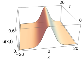
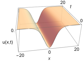
Figure 1: Solution (16) for (a)  $a=b=-c=1$ (hump), and (b)  $a=\frac{9}{10}$, $b=-\frac{11}{10}$, $c=\frac{41}{40}$ (dip).

which appeared earlier in the literature Hunter83 ; Her85 ; Her86 . Fig. 1 illustrates solution (16) for $a=b=-c=1,$ and $a=\frac{9}{10}$, $b=-\frac{11}{10}$, and $c=\frac{41}{40},$ resulting in a hump and a dip, respectively.

III.2 Sech solutions for the seventh-order KdV equation

To find sech solutions for (4) using the expressions in (A.1), we first solve $r_{3}=r_{4}=r_{5}=r_{6}=0$, yielding

$$A_{0}=\text{v}-\frac{231}{50}{a_{2}}^{2}-22\alpha{a_{2}}^{3}+\frac{(334)7^{2}-(681)5^{3}\alpha}{(262)5^{5}\alpha^{2}}+\frac{231(49-500\alpha)a_{2}}{(262)5^{3}\alpha},$$

$$A_{1}=\frac{231(3a_{3})}{(262)5^{3}\alpha}\left[49-50\alpha\left(10-131a_{2}\right)-(524)5^{3}\alpha^{2}{a_{2}}^{2}\right],$$ (17)

$$A_{2}=\frac{231}{10}(3a_{3})^{2}\left(1-50\alpha a_{2}\right),\;\;A_{3}=-385\alpha(3a_{3})^{3}.$$

After substituting these coefficients into $r_{1}=r_{2}=0,$ we must distinguish between two cases: $a_{2}^{+}=\frac{100}{2159},\,\alpha^{+}=\frac{2159}{10^{4}}$ and $a_{2}^{-}=\frac{50}{769},\,\alpha^{-}=\frac{769}{2500}$. Furthermore, $r_{0}=0$ determines the integration constant $\mathcal{C}=\frac{1}{2}A_{0}\left(2\text{v}-A_{0}\right)$ which for the respective cases becomes $\mathcal{C}^{+}=\frac{\text{v}^{2}}{2}-\frac{(5)71^{2}\,10^{7}}{17^{4}\,127^{4}}$ and $\mathcal{C}^{-}=\frac{\text{v}^{2}}{2}-\frac{(2)3^{4}\,10^{8}}{769^{4}}.$

III.2.1 Case $(a_{2}^{+},\,\alpha^{+})$

In this case, system (III.2) gives

$$A_{0}=\text{v}-\frac{(71)10^{4}}{17^{2}127^{2}},\;A_{1}=0,\,A_{2}=-\frac{231}{20}(3a_{3})^{2},\,\mathrm{and}\;\;A_{3}=-\frac{(17)(77)(127)}{(2)10^{3}}(3a_{3})^{3}.$$ (18)

Substituting (11) into (8) yields

$$U(\xi)=\text{v}-\frac{(71)10^{4}}{17^{2}127^{2}}+\frac{(385)3^{3}10^{2}}{17^{2}127^{2}}\,\mathrm{sech}^{4}\eta\,(1+\mathrm{sech}^{2}\eta),$$ (19)

where $\eta=\frac{5(\xi-\xi_{0})}{\sqrt{2159}}$. Eq. (19), in which v and $\xi_{0}$ are arbitrary constants, solves (5) provided $\alpha=\frac{2159}{10^{4}}$ and $\mathcal{C}=\mathcal{C}^{+}$. Converting (19) into the original variables yields

$$u(x,t)= \frac{b^{2}}{17^{2}\,127^{2}ac}\Bigg{\{}(71)10^{4}-17^{2}127^{2}\text{v}-(385)3^{3}10^{2}\,\mathrm{sech}^{4}\left[\frac{5}{\sqrt{2159}}\left(\delta_{1}+\sqrt{-\frac{b}{c}}(x+\frac{b^{2}\text{v}}{c}t)\right)\right]$$ (20)

$$\left\{1+\mathrm{sech}^{2}\left[\frac{5}{\sqrt{2159}}\left(\delta_{1}+\sqrt{-\frac{b}{c}}(x+\frac{b^{2}\text{v}}{c}t)\right)\right]\right\}\Bigg{\}},$$

where both the velocity v and phase constant $\delta_{1}$ are arbitrary. Solution (20) satisfies (1) provided $d=\frac{2159\,c^{2}}{10^{4}\,b}.$ When $A_{0}=0$ the wave speed becomes $\text{v}^{+}=\frac{(71)\,10^{4}}{17^{2}\,127^{2}}\approx 0.1523$ and $\mathcal{C}^{+}=0.$ Physically, this means that the solitary wave solution is not shifted on the vertical axis but tends to zero as $|x|\rightarrow\infty$. Furthermore, for $\delta_{1}=0$ and v replaced by $\text{v}^{+},$ (20) simplifies into

$$u(x,t)= -\,\frac{(385)3^{3}10^{2}\,b^{2}}{17^{2}\,127^{2}ac}\,\mathrm{sech}^{4}\left[\frac{5}{\sqrt{2159}}\sqrt{-\frac{b}{c}}\left(x+\frac{(71)\,10^{4}\,b^{2}}{17^{2}\,127^{2}\,c}t\right)\right]$$ (21)

$$\left\{1+\mathrm{sech}^{2}\left[\frac{5}{\sqrt{2159}}\sqrt{-\frac{b}{c}}\left(x+\frac{(71)\,10^{4}\,b^{2}}{17^{2}\,127^{2}\,c}t\right)\right]\right\}.$$

III.2.2 Case $(a_{2}^{-},\,\alpha^{-})$

For this case, system (III.2) becomes

$$A_{0}=\text{v}-\frac{(18)\,10^{4}}{769^{2}},\;\;A_{1}=0,\;\;A_{2}=0,\;\;\mathrm{and}\;\;A_{3}=-\frac{(77)\,(769)}{500}(3a_{3})^{3}.$$ (22)

Upon substitution of (11) into (8), one gets

$$U(\xi)=\text{v}-\frac{(18)\,10^{4}}{769^{2}}+\frac{(154)\,3^{3}\,5^{3}}{769^{2}}\,\mathrm{sech}^{6}\chi,$$ (23)

where $\chi=\frac{5(\xi-\xi_{0})}{\sqrt{1538}}$. Eq. (23), in which v and $\xi_{0}$ are arbitrary constants, solves (5) provided $\alpha=\frac{769}{2500}$ and $\mathcal{C}=\mathcal{C}^{-}$. In the original variables (23) reads

$$u(x,t)=\frac{b^{2}}{769^{2}ac}\left\{(18)10^{4}-\!769^{2}\text{v}-\!(154)3^{3}5^{3}\,\mathrm{sech}^{6}\left[\!\frac{5}{\sqrt{1538}}\left(\delta_{2}+\!\!\sqrt{-\frac{b}{c}}(x+\!\frac{b^{2}\text{v}}{c}t)\right)\right]\right\},$$ (24)

where both v and $\delta_{2}$ are arbitrary. Solution (24) satisfies (1) provided $d=\frac{769\,c^{2}}{2500\,b}$.

Setting $A_{0}=0$ fixes the wave speed $\text{v}^{-}=\frac{(18)\,10^{4}}{769^{2}}\approx 0.3044$ and $\mathcal{C}^{-}=0$. The solitary wave with speed $\text{v}^{-}$ approaches zero as $|x|\rightarrow\infty$. Setting $\delta_{2}=0$ and replacing v by $\text{v}^{-},$ further simplifies (24) into

$$\begin{array}[]{l}u(x,t)=-\,\frac{(154)3^{3}5^{3}\,b^{2}}{769^{2}\,ac}\,\mathrm{sech}^{6}\left[\frac{5}{\sqrt{1538}}\sqrt{-\frac{b}{c}}\left(x+\frac{(18)\,10^{4}\,b^{2}}{769^{2}\,c}t\right)\right].\end{array}$$ (25)

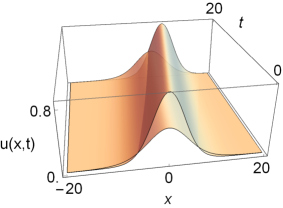
Figure 2: Comparison of solutions (21) (short and wide) and (25) (tall and narrow).

Fig. 2 shows solutions (21) and (25) for $a=b=-c=1,$ resulting in $d=\frac{2159}{10^{2}}$ and $d=\frac{769}{2500},$ respectively. Solitary wave (25) has approximately twice the speed, twice the height, and three-quarters the width of solitary wave (21). Setting $a=\frac{9}{10}$, $b=-\frac{11}{10}$, and $c=\frac{41}{40}$ would lead to a similar picture (not shown) with two dips instead of two humps.

IV Cnoidal Wave Solutions

To obtain cnoidal wave solutions we require that $Y_{\xi}=0$ when $Y=0$ which implies that $Q_{3}(Y)$ should have only one zero root, $Y_{1}=0,$ and two distinct real roots, $Y_{2}$ and $Y_{3}$. This requires that $a_{0}=0.$ Under these assumptions (9) becomes

$${Y_{\xi}}^{2}=a_{1}Y+a_{2}Y^{2}+a_{3}Y^{3}=Y(a_{1}+a_{2}Y+a_{3}Y^{2}),$$ (26)

which can be factored as

$${Y_{\xi}}^{2}=-a_{3}Y(Y_{2}-Y)(Y_{3}+Y).$$ (27)

The solution of (27) is the cnoidal wave KdV

$$Y(\xi)=Y_{2}\,\mathrm{cn}^{2}\left[\frac{1}{2}\sqrt{-a_{3}(Y_{2}+Y_{3})}(\xi-\xi_{0});k\right],$$ (28)

where $\mathrm{cn}(\theta;k)$ is the Jacobi elliptic function with modulus $k=\sqrt{\frac{Y_{2}}{Y_{2}+Y_{3}}}$ and $\xi_{0}$ an arbitrary constant. By equating the coefficients of (26) with (27) we identify the roots, $Y_{2}=-\frac{a_{2}+\sqrt{\Omega}}{2a_{3}},\,Y_{3}=\frac{a_{2}-\sqrt{\Omega}}{2a_{3}},$ with discriminant and modulus given by

$$\Omega={a_{2}}^{2}-4a_{1}a_{3}>0,\quad k=\sqrt{\frac{1}{2}\left(1+\frac{a_{2}}{\sqrt{\Omega}}\right)}.$$ (29)

Thus, the solution of (26) becomes

$$Y(\xi)=-\frac{1}{2}\left(\frac{a_{2}+\sqrt{\Omega}}{a_{3}}\right)\,\mathrm{cn}^{2}\left[\frac{1}{2}\sqrt[4]{\Omega}(\xi-\xi_{0});\sqrt{\frac{1}{2}\left(1+\frac{a_{2}}{\sqrt{\Omega}}\right)}\right],\;\;a_{3}\neq 0.$$ (30)

The expressions of the derivatives of $U$, after substitution of ${Y_{\xi}}^{2}$ from (26) together with all higher order derivatives, are given in (A.2). Substituting these derivatives into (5) results in a sixth-degree polynomial $\sum_{i=0}^{6}s_{i}Y(\xi)^{i},$ which must identically vanish since the powers of $Y(\xi)$ are independent for varying $\xi$. The expressions for the coefficients $s_{i}$ are given in (A.2). The equations, $s_{i}=0,$ are then solved for the $A_{i}$ in terms of the $a_{i},\alpha,$ and $\text{v},$ some of which become constrained. The integration constant ${\mathcal{C}}$ depends on v. Instead of doing this in full generality, we consider special cases corresponding to PDEs of physical relevance.

IV.1 Cn solutions for the fifth-order KdV equation

We now compute cn solutions for (4) with $\alpha=0$. Since $N=2$ in (8), we set $A_{3}=\alpha=0$ in (A.2), discarding $s_{5}$ and $s_{6}.$ Solving $s_{2}=s_{3}=s_{4}=0$ yields the expansion coefficients

$$A_{0}=\text{v}-\frac{31}{507}+42a_{1}a_{3}-\frac{7}{507}p(10+p),\;\;A_{1}=-\frac{70}{13}a_{3}(1-p),\;\;A_{2}=105{a_{3}}^{2},$$ (31)

where $p=13a_{2}$. Solving $s_{1}=s_{0}=0,$ after inserting these coefficients, gives

$$\begin{array}[]{ll}&a_{1}=-\,\frac{(1-p)\left(31+31p+10p^{2}\right)}{117(13a_{3})\left(7+5p\right)},\\ &\mathcal{C}=\frac{7\left[(63)13^{4}\text{v}^{2}-124(677)\right]+5p\left\{42\left[(3)13^{4}\text{v}^{2}-3658\right]-5p\left[9(31)(47)+161p(2-p)\left(2-2p-p^{2}\right)-(9)13^{4}\text{v}^{2}\right]\right\}}{(18)13^{4}(7+5p)^{2}}.\end{array}$$ (32)

Substituting $a_{1}$ from (32) into (29) gives

$$\Omega=\frac{(2+p)\left(62-31p+5p^{2}\right)}{3^{2}13^{2}(7+5p)},\;\;k=\frac{\sqrt{2}}{2}\sqrt{1+3p\sqrt{\frac{7+5p}{(2+p)(62-31p+5p^{2})}}}.$$ (33)

Finally, substituting $a_{1}$ into (31), and these coefficients with (28) into (8), yields

$$U(\xi) = -\,\frac{7(31-13^{2}\text{v})+5p(43-13^{2}\text{v})+35p^{2}(1-p)}{13^{2}(7+5p)}$$ (34)

$$+\,\frac{35}{676}(p+13\sqrt{\Omega})\,\mathrm{cn}^{2}(\eta;k)\big{[}4(1-p)+3(p+13\sqrt{\Omega})\,\mathrm{cn}^{2}(\eta;k)\big{]},$$

where $\eta=\frac{1}{2}\sqrt[4]{\Omega}(\xi-\xi_{0})$ with $\Omega$ and $k$ in (33). Note that for $p=1$, (33) yields $\Omega=\frac{1}{169},k=1,$ and the cnoidal wave (34) becomes the solitary wave (14). Converting (34) into the original variables gives

$$u(x,t) = \frac{b^{2}}{ac}\left\{\frac{7(31-13^{2}\text{v})+5p(43-13^{2}\text{v})+35p^{2}(1-p)}{13^{2}(7+5p)}\right.$$ (35)

$$\left.-\frac{35}{676}(p+13\sqrt{\Omega})\,\mathrm{cn}^{2}(\zeta;k)\big{[}4(1-p)+3(p+13\sqrt{\Omega})\,\mathrm{cn}^{2}(\zeta;k)\big{]}\right\},$$

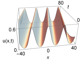
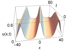
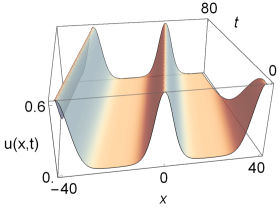
Figure 3: Solution (35) for $a=b=-c=1$,   (a)  $p=0,$ (b)  $p=\frac{3}{4},$ and (c)  $p=\frac{9}{10}.$

where $\zeta=\frac{1}{2}\sqrt[4]{\Omega}\left[\delta_{1}+\sqrt{-\frac{b}{c}}\left(x+\frac{b^{2}\text{v}}{c}t\right)\right]$, satisfies (1) with $d=0$. Eq. (35) expresses a new two-parameter family of solutions since both v and $p$ are arbitrary. Only the solution with $\text{v}=\frac{128}{507}\approx 0.2525$ and $p=0$ yielding $k=\frac{\sqrt{2}}{2}$ has been reported in the literature Manc . As before, we plot the solutions corresponding to $A_{0}=0$ yielding $\text{v}=\frac{217+5p\left[43+7p(1-p)\right]}{169(7+5p)}$. Fig. 3 shows solution (35) for $a=b=-c=1$, with $p=0,\,\frac{3}{4},$ and $\frac{9}{10}$ for which $\text{v}=\frac{31}{169}\approx 0.1834,\,\frac{137(179)}{(43)\,2^{4}\,13^{2}}\approx 0.2109$, and $\frac{6359}{(299)\,10^{2}}\approx 0.2127,$ respectively. The cnoidal waves spread out more as $p$ increases. As $p$ approaches one the cnoidal wave turns into solitary wave (14) with speed $\text{v}=\frac{36}{169}\approx 0.2130$.

IV.2 Cn solutions for the seventh-order KdV equation

To find cnoidal wave solutions for (4) using the expressions in (A.2), we first solve $s_{3}=s_{4}=s_{5}=s_{6}=0$, yielding

$$A_{0}=\text{v}-\frac{231}{50}{a_{2}}^{2}-22\alpha{a_{2}}^{3}+\frac{33}{25}q(7-50\alpha a_{2})+\frac{(334)7^{2}-(681)5^{3}\alpha}{(262)5^{5}\alpha^{2}}+\frac{231(49-500\alpha)a_{2}}{(262)5^{3}\alpha},$$

$$A_{1}=\frac{(77)3^{2}a_{3}}{(262)5^{3}\alpha}\left[49-50\alpha\left(10-131a_{2}\right)-(262)5^{3}\alpha^{2}\left(2{a_{2}}^{2}+q\right)\right],$$ (36)

$$A_{2}=\frac{231}{10}(3a_{3})^{2}\left(1-50\alpha a_{2}\right),\;\;A_{3}=-385\alpha(3a_{3})^{3},$$

where $q=9a_{1}a_{3}.$

Upon substitution of these coefficients into $s_{2}=0,$ we obtain a complicated equation (not shown) of fourth degree in both $\alpha$ and $a_{2}$ and quadratic in $q$. Likewise, $s_{1}=0$ yields an equation of fifth degree in both $\alpha$ and $a_{2}$ and quadratic in $q,$ and $s_{0}=0,$ which would determine ${\mathcal{C}}$, becomes of degree six in both $\alpha$ and $a_{2}$ and cubic in $q$. Inspired by the results in Sect. IV.1, we illustrate the solution procedure for $a_{2}=0.$ The numerical treatment of the general case $(a_{2}\neq 0)$ would be similar but very cumbersome.

For $a_{2}=0,$ from $s_{1}=0$ and $s_{2}=0$ we get

$$6(167)7^{4}-\!125\alpha\left\{3(2017)7^{2}-\alpha\left[(227)6^{2}\,5^{3}-\!77{\tilde{q}}\left(441-\!500\alpha(9-4{\tilde{q}}\alpha)\right)\right]\right\}=0,$$

$$3(37)(2671)7^{2}\!-\!500\alpha\left\{6(101)317\!-\!\alpha\left[6(331)5^{3}\!+\!77{\tilde{q}}\left(147\!-\!250\alpha(6\!-\!{\tilde{q}}\alpha)\right)\right]\right\}=0,$$ (37)

respectively, where ${\tilde{q}}=131q=9(131)a_{1}a_{3}.$

Solving (IV.2) numerically yields the following four real solutions for the couples $({\tilde{q}},\alpha)$: $(-2.4191,0.3075),\,(-1.2262,0.2158),\,(2.2502,1.6115)$, and $(5.6486,0.1912)$. Setting $a_{2}=0$ in (29) gives $\Omega=-4a_{1}a_{3}=-\frac{4{\tilde{q}}}{9(131)}>0$ and $k=\frac{\sqrt{2}}{2},$ requiring ${\tilde{q}}<0$. Using $q=\frac{{\tilde{q}}}{131},$ only

$$(q_{1},\alpha_{1})=(-0.0185,0.3075)\;\;{\rm and}\;\;(q_{2},\alpha_{2})=(-0.0094,0.2158)$$ (38)

will lead to real solutions. We label the solutions below accordingly.

Finally, substituting (IV.2) with $a_{2}=0$ into (8) gives two solutions

$$U_{i}(\xi) = {\text{v}+\frac{231}{25}q_{i}-\frac{681}{2(131)5^{2}\alpha_{i}}+\frac{(167)7^{2}}{(131)5^{5}\alpha_{i}^{2}}}$$ (39)

$$+\,{\frac{(77)3^{2}a_{3}}{(262)5^{3}\alpha_{i}}\Big{(}49-500\alpha_{i}-(262)5^{3}q_{i}{\alpha_{i}}^{2}\Big{)}}Y_{i}(\xi)$$

$$+\,{\frac{231}{10}(3a_{3})^{2}}Y_{i}(\xi)^{2}-{385\alpha_{i}(3a_{3})^{3}}Y_{i}(\xi)^{3},$$

where

$$Y_{i}(\xi)=-\,\frac{\sqrt{-q_{i}}}{3a_{3}}\,\mathrm{cn}^{2}\left[\frac{\sqrt[4]{-q_{i}}}{\sqrt{6}}\Big{(}\xi-\xi_{0}\Big{)};\frac{\sqrt{2}}{2}\right],\;q_{i}<0,\;i=1,2.$$ (40)

In the original variables,

$$u_{i}(x,t) = -\,\frac{b^{2}}{ac}\left\{\text{v}+\frac{231}{25}q_{i}-\frac{681}{2(131)5^{2}\alpha_{i}}+\frac{(167)7^{2}}{(131)5^{5}\alpha_{i}^{2}}\right.$$ (41)

$$\left.-\,{\frac{(231)\sqrt{-q_{i}}}{(262)5^{3}\alpha_{i}}\Big{(}49-500\alpha_{i}-(262)5^{3}q_{i}{\alpha_{i}}^{2}\Big{)}}\,\mathrm{cn}^{2}\left[\zeta_{i};\frac{\sqrt{2}}{2}\right]\right.$$

$$\left.-\,{\frac{231q_{i}}{10}}\,\mathrm{cn}^{4}\left[\zeta_{i};\frac{\sqrt{2}}{2}\right]-\,{385\alpha_{i}q_{i}\sqrt{-q_{i}}}\,\mathrm{cn}^{6}\left[\zeta_{i};\frac{\sqrt{2}}{2}\right]\right\},\;q_{i}<0,\;i=1,2,$$

where $\zeta_{i}=\frac{\sqrt[4]{-q_{i}}}{\sqrt{6}}\left[\delta_{i}+\sqrt{-\frac{b}{c}}\left(x+\frac{b^{2}\text{v}}{c}t\right)\right]$, satisfying (1) provided $d=d_{i}=\frac{c^{2}\alpha_{i}}{b},$ and with $(q_{i},\alpha_{i})$ given in (38). Ignoring the phase constant $\delta_{i}$, each solution in (41) defines a one-parameter family of solutions since v is arbitrary. To our knowledge, solutions of type (41) have not been reported in the literature. To remove the constant term in (41), we set $\text{v}_{i}=\frac{375\alpha_{i}\left[227-131(154)q_{i}\alpha_{i}\right]-(334)\,7^{2}}{(262)\,5^{5}\alpha_{i}^{2}}$, and from $(\ref{qialphaicn7thKdV})$ we then have $\text{v}_{1}\approx 0.2973$ and $\text{v}_{2}\approx 0.1391$, respectively. These solutions are presented in Fig. 4 for $a=b=-c=1$.

V Discussion and Conclusions

In this paper we surveyed the origin and applications of a KdV equation with higher-order dispersive terms. Specific members of this parameterized family of equations describe shallow water waves, electrical pulses in transmission lines, magneto-acoustic and hydrodynamic waves in plasmas, etc. Using an elliptic function method, we computed hump-type solitary waves and cnoidal wave solutions which can be used in bifurcation analyses and as benchmarks for both numerical solvers and perturbation methods.

Some of the solutions presented in this paper correct, complement, and illustrate results previously reported in the literature. Solution (20) was missed by Ma Ma but later computed by Duffy and Parkes Duffy . Solution (24) is equivalent to a solution reported by Ma Ma . However, solution (6) on p. 222 in Ma’s paper Ma should have read

$$u(x,t)=-\frac{519750\,b^{2}}{769^{2}\,ac}\,\mathrm{sech}^{6}\left\{\sqrt{-\frac{25\,b}{1538\,c}}\left[x-\left(aE-\frac{180000\,b^{2}}{769^{2}\,c}\right)t-\xi_{0}\right]\right\}+E,$$ (42)

where $E$ and $\xi_{0}$ are arbitrary constants. To convert (42) into (24), set $E=\frac{b^{2}}{769^{2}\,ac}\left(180000-769^{2}\,\text{v}\right)$ and $\delta_{2}=\sqrt{-\frac{b}{c}}\,\xi_{0}.$

Solutions (20) and (24) to (1) are the only polynomial solutions involving the sech-function. Both require that the coefficients in (1) satisfy specific algebraic relations. Application of the tanh- or sech-method Bald to (4) results in expressions which are equivalent to (19) and (23) as verified with the Mathematica package PDESpecialSolutions.m BaldSoft . To our knowledge, solutions (35) and (41) are novel although a special case of (35) had been reported Manc . Solutions as complicated as (35) and (41) are beyond the present capabilities of PDESpecialSolutions.m.

Finally, all solutions reported in this paper have been verified with Mathematica which uses the square of the modulus (denoted by $k$ in this paper) of the Jacobi elliptic functions.

Figures

.

.

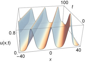
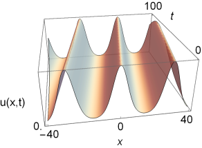
Figure 4: Solution (41) for $a=b=-c=1$ for (a)  $q_{1}=-0.0185,\,\alpha_{1}=0.3075,\,\text{v}_{1}=0.2973,$ and (b)  $q_{2}=-0.0094,\,\alpha_{2}=0.2158,\,\text{v}_{2}=0.1391.$

Appendix A

A.1 Formulas needed to compute sech solutions

$$U_{2\xi}=\frac{Y}{2}\left[2A_{1}a_{2}+\left(8A_{2}a_{2}+3A_{1}a_{3}\right)Y+2\left(5A_{2}a_{3}+9A_{3}a_{2}\right)Y^{2}+21A_{3}a_{3}Y^{3}\right],$$

$$U_{4\xi}=\frac{Y}{2}\left[2A_{1}{a_{2}}^{2}+a_{2}\left(32A_{2}a_{2}+15A_{1}a_{3}\right)Y+\left(130A_{2}a_{2}a_{3}+15A_{1}{a_{3}}^{2}+162A_{3}{a_{2}}^{2}\right)Y^{2}\right.$$

$$\left.\;\;\;\;\;\;\;\;\;+105a_{3}\left(A_{2}a_{3}+5A_{3}a_{2}\right)Y^{3}+378A_{3}{a_{3}}^{2}Y^{4}\right],$$ (A.1)

$$U_{6\xi}=\frac{Y}{4}\left[4A_{1}{a_{2}}^{3}+2{a_{2}}^{2}\left(128A_{2}a_{2}+63A_{1}a_{3}\right)Y+4a_{2}\left(665A_{2}a_{2}a_{3}+105A_{1}{a_{3}}^{2}\right.\right.$$

$$\left.\left.\;\;\;\;\;\;\;\;\;+A_{3}{(27a_{2})}^{2}\right)Y^{2}+21a_{3}\left(290A_{2}a_{2}a_{3}+15A_{1}{a_{3}}^{2}+962A_{3}{a_{2}}^{2}\right)Y^{3}\right.$$

$$\left.\;\;\;\;\;\;\;\;\;+105(6a_{3})^{2}\left(A_{2}a_{3}+10A_{3}a_{2}\right)Y^{4}+770A_{3}(3a_{3})^{3}Y^{5}\right].$$

$$r_{0}=\frac{A_{0}}{2}(2\text{v}-A_{0})-\mathcal{C},$$

$$r_{1}=A_{1}\left[\text{v}-A_{0}-a_{2}(1-a_{2}+\alpha{a_{2}}^{2})\right],$$

$$r_{2}=-\frac{A_{1}}{2}\left[A_{1}+3a_{3}\left(1-5a_{2}+21\alpha{a_{2}}^{2}\right)\right]+A_{2}\left[\text{v}-A_{0}-4a_{2}\left(1-4a_{2}+16\alpha{a_{2}}^{2}\right)\right],$$

$$r_{3}=A_{1}\left[\frac{15}{2}{a_{3}}^{2}(1-14\alpha a_{2})-A_{2}\right]-5A_{2}a_{3}\left(1-13a_{2}+133\alpha{a_{2}}^{2}\right)$$

$$\;\;\;\;\;\;\;+A_{3}\left[\text{v}-A_{0}-9a_{2}\left(1-9a_{2}+81\alpha{a_{2}}^{2}\right)\right],$$ (A.2)

$$r_{4}=-A_{1}\left(A_{3}+\frac{315}{4}\alpha{a_{3}}^{3}\right)-\frac{{A_{2}}}{2}\left[A_{2}-105{a_{3}}^{2}\left(1-29\alpha a_{2}\right)\right]$$

$$\;\;\;\;\;\;\;-\frac{21}{2}A_{3}a_{3}\left(1-25a_{2}+481\alpha{a_{2}}^{2}\right),$$

$$r_{5}=-A_{2}\left[A_{3}+35\alpha{(3a_{3})}^{3}\right]+21A_{3}{(3a_{3})}^{2}\left(1-50\alpha a_{2}\right),$$

$$r_{6}=-\frac{A_{3}}{2}\left[A_{3}+385\alpha(3a_{3})^{3}\right].$$

A.2 Formulas needed to compute cn solutions

$$U_{2\xi}=\frac{1}{2}\left[A_{1}a_{1}+2\left(A_{1}a_{2}+3A_{2}a_{1}\right)Y+\left(3A_{1}a_{3}+8A_{2}a_{2}+15A_{3}a_{1}\right)Y^{2}\right.$$

$$\left.\;\;\;\;\;\;\;\;\;+2\left(5A_{2}a_{3}+9A_{3}a_{2}\right)Y^{3}+21A_{3}a_{3}Y^{4}\right],$$

$$U_{4\xi}=\frac{1}{2}\left\{a_{1}\left(A_{1}a_{2}+3A_{2}a_{1}\right)+\left[A_{1}\left(2{a_{2}}^{2}+9a_{1}a_{3}\right)+30A_{2}a_{1}a_{2}+45A_{3}{a_{1}}^{2}\right]Y\right.$$

$$\left.\;\;\;\;\;\;\;\;\;+\left[15a_{2}(A_{1}a_{3}+13A_{3}a_{1})+4A_{2}(8{a_{2}}^{2}+21a_{1}a_{3})\right]Y^{2}\right.$$

$$\left.\;\;\;\;\;\;\;\;\;+\left[5a_{3}(3A_{1}a_{3}+26A_{2}a_{2})+9A_{3}(18a_{2}^{2}+41a_{1}a_{3})\right]Y^{3}\right.$$

$$\left.\;\;\;\;\;\;\;\;\;+105{a_{3}}(A_{2}a_{3}+5A_{3}a_{2})Y^{4}+378A_{3}{a_{3}}^{2}Y^{5}\right\},$$

$$U_{6\xi}=\frac{1}{4}\left\{a_{1}\left[2A_{1}{a_{2}}^{2}+3a_{1}(3A_{1}a_{3}+10A_{2}a_{2}+15A_{3}a_{1})\right]\right.$$ (A.3)

$$\left.\;\;\;\;\;\;\;\;\;+4\left[A_{1}a_{2}\left(27a_{1}a_{3}+{a_{2}}^{2}\right)+63a_{1}\left(A_{2}(2a_{1}a_{3}+{a_{2}}^{2})+5A_{3}a_{1}a_{2}\right)\right]Y\right.$$

$$\left.\;\;\;\;\;\;\;\;\;+2\left[4A_{2}a_{2}\left(339a_{1}a_{3}+32{a_{2}}^{2}\right)+63a_{1}a_{3}(2A_{1}a_{3}+45A_{3}a_{1})\right.\right.$$

$$\left.\left.\;\;\;\;\;\;\;\;\;+21{a_{2}}^{2}(3A_{1}a_{3}+95A_{3}a_{1})\right]Y^{2}\right.$$

$$\left.\;\;\;\;\;\;\;\;\;+4\left[35A_{2}a_{3}\left(27a_{1}a_{3}+19{a_{2}}^{2}\right)+729A_{3}{a_{2}}^{3}+3a_{2}a_{3}(35A_{1}a_{3}+1941A_{3}a_{1})\right]Y^{3}\right.$$

$$\left.\;\;\;\;\;\;\;\;\;+21a_{3}\left[2a_{2}(145A_{2}a_{3}+481A_{3}a_{2})+3a_{3}(5A_{1}a_{3}+393A_{3}a_{1})\right]Y^{4}\right.$$

$$\left.\;\;\;\;\;\;\;\;\;+105{(6a_{3})}^{2}(A_{2}a_{3}+10A_{3}a_{2})Y^{5}+770A_{3}(3a_{3})^{3}Y^{6}\right\}.$$

$$s_{0}=\frac{A_{0}}{2}(2\text{v}-A_{0})-\mathcal{C}$$

$$\;\;\;\;\;\;\;\;\;-\frac{a_{1}}{2}\left[A_{1}\left(1-a_{2}+\alpha{a_{2}}^{2}+\frac{9}{2}\alpha a_{1}a_{3}\right)-3A_{2}a_{1}\left(1-5\alpha a_{2}\right)+\frac{45}{2}A_{3}\alpha{a_{1}}^{2}\right],$$

$$s_{1}=A_{1}\left[\text{v}-A_{0}-a_{2}(1-a_{2}+\alpha{a_{2}}^{2}+27\alpha a_{1}a_{3})+\frac{9}{2}a_{1}a_{3}\right]$$

$$\;\;\;\;\;\;\;\;\;-3a_{1}\left[A_{2}\left(1-5a_{2}+21\alpha({a_{2}}^{2}+2a_{1}a_{3})\right)-\frac{15}{2}A_{3}a_{1}(1-14\alpha a_{2})\right],$$

$$s_{2}=-\frac{A_{1}}{2}\left[A_{1}+3a_{3}\left(1-5a_{2}+21\alpha({a_{2}}^{2}+2a_{1}a_{3})\right)\right]$$

$$\;\;\;\;\;\;\;\;\;+A_{2}\left[\text{v}-A_{0}-4a_{2}(1-4a_{2}+16\alpha{a_{2}}^{2})+6a_{1}a_{3}(7-113\alpha a_{2})\right]$$

$$\;\;\;\;\;\;\;\;\;-\frac{15}{2}A_{3}a_{1}\left[1-a_{2}(13-133\alpha a_{2})+189\alpha a_{1}a_{3}\right],$$ (A.4)

$$s_{3}=A_{1}\left[\frac{15}{2}{a_{3}}^{2}(1-14\alpha a_{2})-A_{2}\right]-5A_{2}a_{3}\left[1-13a_{2}+7\alpha(19{a_{2}}^{2}+27a_{1}a_{3})\right]$$

$$\;\;\;\;\;\;\;\;\;+A_{3}\left[\text{v}-A_{0}-9a_{2}\left(1-9a_{2}+81\alpha{a_{2}}^{2}+647\alpha a_{1}a_{3}\right)+\frac{369}{2}a_{1}a_{3}\right],$$

$$s_{4}=-A_{1}(A_{3}+\frac{315}{4}\alpha{a_{3}}^{3})-\frac{A_{2}}{2}\left[A_{2}-105{a_{3}}^{2}(1-29\alpha a_{2})\right]$$

$$\;\;\;\;\;\;\;-\frac{21}{2}A_{3}a_{3}\left[1-25a_{2}+481\alpha{a_{2}}^{2}+\frac{1179}{2}\alpha a_{1}a_{3}\right],$$

$$s_{5}=-A_{2}\left[A_{3}+35\alpha{(3a_{3})}^{3}\right]+21A_{3}{(3a_{3})}^{2}\left(1-50\alpha a_{2}\right),$$

$$s_{6}=-\frac{A_{3}}{2}\left[A_{3}+385\alpha(3a_{3})^{3}\right].$$