Examining the neutrino option
Abstract
The neutrino option is a scenario where the electroweak scale, and thereby the Higgs mass, is generated simultaneously with neutrino masses in the seesaw model. This occurs via the leading one loop and tree level diagrams matching the seesaw model onto the Standard Model Effective Field Theory. We advance the study of this scenario by determining one loop corrections to the leading order matching results systematically, performing a detailed numerical analysis of the consistency of this approach with Neutrino data and the Standard Model particle masses, and by examining the embedding of this scenario into a more ultraviolet complete model. We find that the neutrino option remains a viable and intriguing scenario to explain the origin of observed particle masses.
1 Introduction
The origin of the Higgs potential and the observed neutrino masses are two outstanding questions unanswered by the Standard Model (SM). The smallness of neutrino masses compared to the masses of the quarks and Electroweak gauge bosons can be naturally accommodated in the Seesaw model Minkowski:1977sc ; GellMann:1980vs ; Mohapatra:1979ia ; Yanagida:1980xy ; Schechter:1980gr . In this approach, the neutrino-quark mass hierarchy follows from a separation of the scale (denoted ) associated with a lepton number violating sector leading to neutrino masses, compared to the Electroweak scale () associated with the remaining SM field content.
If the Seesaw model generates neutrino masses, the sensitivity of the Higgs mass term to can lead to a curious tuning of Lagrangian parameters. Such parameter tuning can be avoided – if the Majorana mass scale and couplings are of a particular form Vissani:1997ys ; Brivio:2017dfq . For the same region of parameter space, the Seesaw model can be a phenomenologically viable boundary condition for the Higgs potential, while supplying an origin for the Electroweak scale as a descendent from the scale Brivio:2017dfq . What leads to the Higgs phase of the SM in this case, is Fermi statistics in the leading one loop matching contribution from the seesaw model to the SM potential terms. This matching necessarily occurs while Neutrino masses are generated by the leading tree level matching, as the Majorana states are integrated out. This is the “neutrino option” for generating neutrino masses and the Higgs potential.
The purpose of this paper is to examine this scenario in more numerical and theoretical detail than Ref. Brivio:2017dfq and to illustrate how this scenario can be embedded in more concrete Ultraviolet (UV) models.111As this paper was being drafted, the neutrino option was embedded in a classically conformal UV physics scenario by Brdar et al Brdar:2018vjq . We discuss this interesting proposal in some detail and extend it to include gravitational interactions. We consider the minimal case that can lead to a successful lower energy neutrino phenomenology with two heavy Majorana states leading to two massive light neutrinos.
The outline of this paper is as follows. In Section 2 we define our notation and conventions for the Seesaw model and the leading tree level matching onto the Standard Model Effective Field Theory (SMEFT). In Section 3 we develop the theoretical framework to study the neutrino option at next to leading order (NLO) accuracy, determining the relevant one loop matching into the seesaw model, and discuss the one loop running of the neutrino parameters. In Section 4 we report numerical results fixing the low scale neutrino parameters and Higgs mass as inputs, and determine the parameter required at the matching scale for the scenario to be self consistent. In Section 5 we examine and extend the embedding of the neutrino option into a classically (i.e. massless particle spectrum at leading order) conformal UV completion, as recently proposed by Brdar et al Brdar:2018vjq . We discuss the cut off scale in this particular UV embedding and the potential to avoid fine tuning. We briefly comment on the possibility that this UV framework can simultaneously provide a Dark Matter candidate, and in Section 6 we conclude.
2 Theoretical framework
The physics of the SM is such that global lepton number conservation can provide an accidental symmetry protection mechanism for the Higgs potential terms. The operator dimension in the SM, or the SMEFT operator expansion leads to the association of an operators dimension being even (odd) if is even (odd)deGouvea:2014lva ; Kobach:2016ami due to the nature of the SM field content. Here and are the baryon and lepton number violation of the operator considered. is of even dimension with . Lepton number carrying fields, associated with the mass scale , either couple in pairs to , or with a dimensionful coupling expected to be proximate to , if parameter tuning is avoided. Tree level exchanges leading to then have a cancellation of the introduced dependence (up to ratios of couplings). The coupling of lepton number violating fields also takes place through the portal interaction (+ h.c.). A heavy scale associated with lepton number violating fields leads to an inverse dependence on this scale at tree level, starting with the () dimension five Weinberg operator, due to these interactions222Note that in models with multiple BSM scales, such as the well-known inverse seesaw model Mohapatra:1986aw ; Mohapatra:1986bd ; Bernabeu:1987gr , it is possible to make distinct from the quantity that controls the lepton number violation. In this case the latter can be naturally very small and suppress the Wilson coefficients multiplicatively, while allowing lower values of ( TeV).. The minimal scenario of this form is the Seesaw model of neutrino mass generation. An expectation is that small neutrino masses result, made only smaller by any small couplings to heavy particles. Simultaneously, additive contributions to the Higgs mass parameter appear at one loop . These loop corrections are not forbidden, as lepton number is an accidental symmetry.
The basic pattern of mass scales associated with the Electroweak scale, Higgs mass and neutrino masses can then be
| (1) |
and the Seesaw model parameter space and , which leads to and , is particularly interesting.333For related results see Ref. Davoudiasl:2014pya ; Casas:1998cf ; Casas:1999cd ; Bambhaniya:2016rbb .
This is the pattern of masses expected when the neutrino option is used to generate the Higgs potential. The idea is to use a UV boundary condition to generate the Higgs potential and an effective Electroweak scale. The smallness of the Higgs mass parameter is linked to the small neutrino masses and a set of approximate symmetries: global lepton number and scale invariance. For the latter, an expansion around the approximately scale invariant limit of the SM444In this work we use scale invariance and conformal invariance interchangeably as we are considering tree level effects of this symmetry, see Refs. Callan:1970ze ; Coleman:1970je for foundational discussions. Ref. Bardeen:1995kv is the first reference, to our knowledge, discussing the use of scale invariance to address the Hierarchy problem. Scale invariance is of course anomalous Capper:1974ic , but still useful to consider in this manner., incorporating the soft breaking of approximate scale invariance feeding into the Higgs potential due to the scale is done. (In the limit , .) We stress however, that the excitation of the Higgs field is not the dilaton of spontaneously broken scale invariance in this approach.
The motivation to consider this possible origin of the Electroweak scale is largely supplied by current experimental results. Neutrino’s are known to be massive states, requiring an extension of the SM. It is natural to consider the effects of extending the SM to generate Neutrino masses on the Higgs. Generating the Higgs potential around the scales probed by LHC, with partner states associated with the multiplets of an approximate stabilizing symmetry (such as SUSY), or through lowering the effective Planck scale, is now subject to increasingly severe experimental bounds.555For a good discussion on the theoretical challenges of generating the Higgs potential around the scale in composite models, see Ref. Bellazzini:2014yua . Conversely, the neutrino option uses the running of the Higgs potential parameters in conjunction with threshold matchings required for Neutrinos to have mass when generating the Higgs potential. This occurs at scales far above the observed Higgs mass and generates an effective Electroweak scale with scant experimental evidence of any stabilizing symmetry.666In such a scenario, technical fine tuning can be avoided, while new states are absent at the LHC. It is also possible that an experimental signature of new scalar states could exist in exceptional regions of parameter space. We discuss this possibility in Section 5.4. The advantage of this approach is that a simple spectra of new physics states, motivated out of the experimental fact that neutrino’s are massive can lead to the observed "mexican-hat" potential at lower scales, once the Higgs potential is run down using the Renormalization Group Equations (RGE) of the SM. A bare value of is required, in addition to the threshold matching contribution to from the seesaw model. This is the main result of this paper’s numerical study. As the Higgs is not a pseudo-Goldstone boson of any symmetry – a bare parameter is also not forbidden.
2.1 The SMEFT
We study the neutrino option in the SMEFT Buchmuller:1985jz ; Grzadkowski:2010es , where the SM is extended with higher dimensional operators to capture the low energy limit of the seesaw model
| (2) |
Here are suppressed by powers of the Majorana scale , that acts as the cut-off, and the are the Wilson coefficients. Our SM notation is consistent with the SMEFT review Brivio:2017vri except for the modified notation for the Higgs potential terms
| (3) | |||||
and the star superscript is generally reserved for complex conjugation on bosonic quantities. Here the bare parameters are . In a classical conformal limit for the mass spectrum of the SM (with non conformal renormalized couplings) while is unconstrained. For the Weinberg operator Weinberg:1979sa ; Wilczek:1979hc we use the notation
| (4) |
Our spinor conventions are that the superscript corresponds to a charge conjugated Dirac four-component spinor with in the chiral basis for the we use. Chiral projection and do not commute so we fix notation that denotes a doublet lepton field chirally projected and subsequently charge conjugated.
2.2 Seesaw model
We use the notation and conventions of Refs. Broncano:2002rw ; Elgaard-Clausen:2017xkq for the Seesaw model. In the Seesaw model, the SM Lagrangian field content is extended with right handed singlet fields with vanishing charges. As these are singlet fermion fields they have Majorana mass terms Majorana:1937vz of the form
| (5) |
where the charge conjugate of is . We define a field satisfying the Majorana condition as in its mass eigenstate basis as Bilenky:1980cx ; Broncano:2002rw
| (6) |
With this choice, all Majorana phases shifted into the effective couplings and the relevant terms in the UV Lagrangian are
| (7) |
Here runs over the heavy Majorana states (), while runs over the SM lepton flavors. This formulation of the Seesaw model is mathematically equivalent to the formulation where
| (8) |
In this case, the Lagrangian is reduced using the charge conjugation identities and the Majorana condition for the field . Comparing calculations in these two formulations beyond tree level uncovers an interesting subtlety in using the Wick expansion, which is discussed in the Appendix.
2.2.1 matching
is a matrix, related to the physical light neutrino masses and mixings via matching onto the Weinberg operator
| (9) |
Expanding the Higgs field around its classical background field gives
and are the mass eigenstates of the light neutrinos . The matrix rotates the neutrinos from their weak eigenstates to their mass eigenstates. Similarly, the matrix rotates between the charged lepton weak and mass eigenstates. These rotations are not the same in general, leading to physical effects due to an overlap matrix being present in the lepton doublet field . This is the Pontecorvo-Maki-Nakagawa-Sakata (PMNS) matrix Pontecorvo:1957cp ; Maki:1962mu defined as
| (10) |
The three eigenvectors in form a basis for the field , as they diagonalize , a Hermitian positive matrix defined over . As the physical effects of the matrix come about due to the relative orientation of the eigenvectors defining and , we can choose the eigenvectors of such that as a basis for this space, so long as no physical conclusions depend on this choice. We use the parameterization
| (11) |
where .
The matrix has two non-zero eigenvalues in the case we consider. The lightest neutrino is massless, which is consistent with experimental results, and the mass eigenstates are labeled in descending order of mixing with the flavor eigenstate. With a Normal Hierarchy (NH) in masses one has then , while for an Inverted Hierarchy (IH) one has . The two remaining masses are related to the squared mass differences defined in Refs. Gonzalez-Garcia:2014bfa ; Esteban:2016qun as777This notation can be related to that of the PDG with for NH/IH.
| (12) |
The notation is such that is the largest mass splitting eigenvalue in the case of either mass ordering. for a NH and for an IH.
2.2.2 Casas-Ibarra parameterization for
The parameter can be written as a function of the light neutrino masses, the PMNS angles and phases, and the heavy Majorana masses , using the Casas-Ibarra parameterization Casas:2001sr . This is a general result whose derivation makes use of the relations in the previous section. In our case, it reads888The factor follows from the conventions chosen above.
| (13) | ||||
| (14) |
for the normal and inverted hierarchy respectively. The matrix is orthogonal and can be parameterized as
| (15) |
so that the rightmost sub-block is orthogonal. The values of dictate the relation between measured low energy neutrino parameters and the Lagrangian parameters. Large values of correspond to parameter space where the and are related as
| (16) |
The eigenvalues of result from a significant degree of cancellation between Lagrangian parameters as a result of this condition being enforced. Interestingly, the latter emerges naturally if the Majorana states , are assumed to form a pseudo-Dirac pair, thereby imposing an approximate lepton number conservation Ibarra:2011xn . In the absence of such a symmetry, however, these relations are not invariant under the RGE of the theory, and therefore represent tuned solutions. To keep the discussion general, in the following we restrict to values .
3 Phenomenology of the neutrino option at NLO
Integrating out the states at one loop gives a threshold matching to the SMEFT Lagrangian parameters proportional to and . These threshold matchings are used to generate the Higgs potential in the neutrino option, so a consistent treatment of the corrections at one loop order is of interest. A more complete treatment of this matching than Ref. Brivio:2017dfq at next to leading order includes all corrections which result from Fig. 1 and the inclusion of the effects of the running of the Weinberg operator. It is also necessary to utilize an alternative numerical strategy than pursued in Ref.Brivio:2017dfq to increase the numerical stability of the results. We first develop a consistent NLO framework for studying the neutrino option in this section.
3.1 One loop matching
The one loop matching of the seesaw model onto the SMEFT is given by equating
| (17) |
for fixed initial () and final () states at the scale , and solving for the resulting SMEFT parameters. This determines the Wilson coefficients of the higher dimensional operators and defines contributions to the SM couplings due to matching boundary conditions.
We calculate in dimension regularization with , and use subtraction. The counterterms renormalize the theories separately on each side of the matching equations, but finite one loop matching results remain.

When matching the propagators used are canonically normalized. The first diagram in Fig. 1a leads to a non-canonical field. A canonical normalization condition can be satisfied by performing a finite renormalization field redefinition of the form
| (18) |
for the matrix element in Eqn.(17). Here the and superscripts correspond to the un-renormalized and renormalized fields respectively in the on-shell matrix elements in the seesaw model, and
| (19) |
We have expanded in where is the value of the Higgs mass parameter before threshold matching and have fixed due to the state which will be taken on-shell in the threshold matching. Similarly Fig. (1)b leads to a non-canonical kinetic term for which is restored with the finite renormalization field redefinition
| (20) |
where
| (21) |
Similarly the non-canonical kinetic term for is restored with the finite renormalization field redefinition where
| (22) |
The three point interactions coupling to the SM are corrected at one loop. For example, one of the interaction terms has the one loop correction
| (23) |
where
| (24) |
Note that this diagram violates lepton number. The corrections for the remaining three point interactions are similar and these (numerically small) effects are required for a complete one loop treatment of the matching of the seesaw model into the SMEFT. The threshold corrections to the SM Higgs potential are999Here we correct an intermediate result in Ref. Brivio:2017dfq . We thank Vedran Brdar for pointing out the correction.
| (25) | ||||
| (26) |
where is the -th row of . Restricting to the case of 2 massive right-handed neutrinos: in the degenerate limit and evaluating at the thresholds to be consistent with the extraction of the threshold correction from the effective potential in 101010See Refs. Casas:1998cf ; Casas:1999cd for related results in the effective potential approach., the result takes the form
| (27) | ||||
| (28) |
In the more general case, we sum the contributions for evaluated at , that for evaluated at to be consistent and the mixed term in evaluated at (where both fields are still dynamical), obtaining:
| (30) |
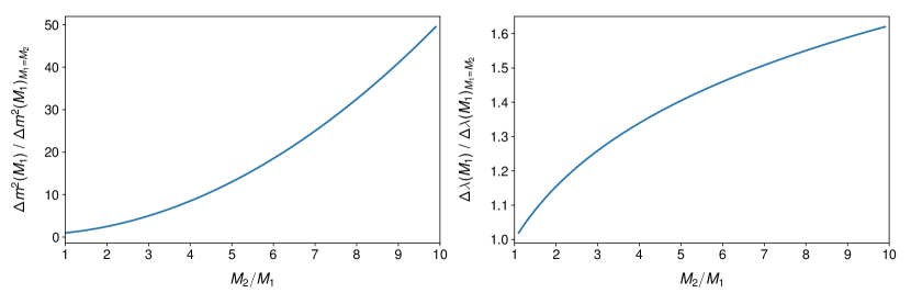
Fig. 2 shows how the thresholds change assuming relative to the degenerate case, as a function of . For definiteness we have fixed and , but the variation has little dependence on this choice.
The net effect of a consistent one loop matching to the seesaw scenario () gives the SMEFT at the matching scale with the Wilson coefficients
with summed over the active states, when each mass eigenstate Majorana field is integrated out. and are the tree level masses of the states. The potential after the one loop matching is given by
| (32) |
We do not assume that hierarchies among the , or significant effects due to their orientation in flavour space in order to enhance the importance of these one loop corrections. Further, we assume is negligible as we are considering a classically scaleless mass spectrum. In the numerical results presented we absorb the correction to into the leading order parameters as a result and neglect the correction to .111111The one loop results given here can be compared to some overlap with past results in the literature given in Refs. Grimus:1989pu ; Grimus:2002nk ; Dev:2012sg ; Fernandez-Martinez:2015hxa . We adopt this approach as these corrections are smaller than the remaining numerical uncertainties in the RGE evolution of the SMEFT parameters.
3.2 Running
The SM potential parameters are compared to measured values run to the scale . For the RGE of the SM we use results from Appendix B of Ref. Buttazzo:2013uya and evaluate the running of as a coupled system, using the RGE computed at loops. The results in Ref. Buttazzo:2013uya allow numerical studies of the order for (without dependence) and up to for .
3.3 Neutrino parameter running
The seesaw model matched onto is compared to the values of masses and mixing angles extracted at after running the seesaw parameters with one loop RGE evolution of the Weinberg operator.121212Here a hat superscript indicates a experimentally measured quantity. The RGEs of the coefficient are extracted from Refs. Babu:1993qv ; Antusch:2001ck . Below the scale the neutrino parameters do not run significantly, as we have explicitly verified.
The RGE of the coefficient is Babu:1993qv ; Antusch:2001ck :
| (33) | ||||
The Yukawa coupling normalization is . In this limit, there is no mixing between the different entries of and the individual elements run according to
| (34) |
Comparing the extracted eigensystem of at any given scale to experimental results in parameter scans is numerically unstable. Using the -functions of the measurable neutrino parameters themselves reduces this numerical uncertainty. We use the results in Ref. Casas:1999tg for a generic parameterization131313Corrected by a factor of three reported in Ref. Antusch:2001ck . of the measurable parameters extracted from . For a normal hierarchy141414These expressions have been derived from the general parameterization in Ref. Casas:1999tg imposing . The case for inverted hierarchy can be inferred analogously, choosing . with two nonzero masses, the results in Ref. Casas:1999tg reduce to
| (35) | ||||
| (36) | ||||
| (37) | ||||
| (38) |
Here we have used the notation
| (39) |
The remaining RGEs are
| (40) | ||||
| (41) | ||||
| (42) |
where denotes the corresponding entry of the matrix defined in Eq. (11).
Ref. Casas:1999tg defined the running of three unphysical phases, that are added to the definition of the rotation such that
| (43) |
This approach is convenient as the field redefinitions that reduce the phases of the PMNS matrix to the minimal set must be re-imposed at each scale . The functions of the unphysical phases are
| (44) | ||||
| (45) | ||||
| (46) |
We have verified analytically that
| (47) |
The running of neutrino parameters depends on . In the numerical results, these are fixed to their value at neglecting yet higher order running effects. Although the running of the neutrino parameters was studied for completeness in the numerical results shown, we confirm past results that find the neutrino parameters do not run in a numerically significant manner. We have verified that the dependence on the top quark mass in the numerical running of the neutrino parameters is a negligible effect when scanning parameter space.
4 Numerical strategy and results
Consistency of the neutrino option explaining the Higgs potential and Neutrino masses is dictated by choosing a subset of inputs among
| (48) |
and predicting the remaining quantity(ies). In Ref. Brivio:2017dfq a consistency test was formulated where was fixed, and it was shown that parameters can be chosen such that can be approximately reproduced. It was observed that significant numerical instability is present in this approach. It is necessary to avoid an asymptotic value of being used as an input for numerical precision. In a consistency test, any mismatch between a predicted value of a parameter, and an observed value can be accommodated by an extended scenario where the Neutrino option is embedded in a UV theory. Only the parameter can receive further classical tree level contributions without breaking a symmetry or adding field content to the scenario. For these reasons, in this paper we formulate a consistency test where are fixed as inputs, and the required is then compared to .
4.1 Numerical inputs
We enforce that the low energy neutrino parameters taken from the global fit in Ref. Esteban:2016qun
| Normal Hierarchy | Inverted Hierarchy | |||
| best fit | range | best fit | range | |
| 0.441 | 0.385 – 0.635 | 0.587 | 0.393 – 0.640 | |
| 0.02166 | 0.01934 – 0.02392 | 0.02179 | 0.01953 – 0.02408 | |
| 0.306 | 0.271 –0.345 | 0.306 | 0.271 – 0.345 | |
| 261 | 0 – 360 | 277 | 145 – 391 | |
| 7.50 | 7.03 – 8.09 | 7.50 | 7.03 – 8.09 | |
| 2.524 | 2.407 – 2.643 | -2.514 | (-2.635) – (-2.399) | |
and given in Table. 1 are reproduced.
The SM parameters are extracted from Ref. Buttazzo:2013uya solving the reported integral equations for the input parameters at the indicated loop order. The light bottom and Yukawa’s, , are matched at tree level as higher order corrections are negligible. The value of is extracted from Eqn. 60 of Ref. Buttazzo:2013uya which includes higher order QCD corrections.
To these SM results we add the effects of the seesaw model as matched onto the SMEFT. The results in Ref. Elgaard-Clausen:2017xkq characterize the tree level matching of the seesaw model onto the SMEFT up to sub-leading order ( corrections) but we restrict our attention to the matching onto in this work.
| best fit | range | |
|---|---|---|
| [GeV-2] | 1.1663787 | |
| 0.1185 | ||
| [GeV] | 91.1875 | |
| [GeV] | 80.387 | |
| [GeV] | 125.09 | |
| [GeV] | 173.2 | 171 – 175 |
| [GeV] | 4.18 | |
| [GeV] | 1.776 |
| tree | 1-loop | 2-loop | |
|---|---|---|---|
| 0.1291 | 0.1276 | 0.1258 | |
| [GeV] | 125.09 | 132.288 | 131.431 |
| 0.451 | 0.463 | 0.461 | |
| 0.653 | 0.6435 | 0.644 | |
| —— 1.22029 —— | |||
| 0.995 | 0.946 | 0.933 | |
| 0.024 | - | - | |
| 0.0102 | - | - | |
The are required to reproduce the observed neutrino masses and mixings. The range of values for compatible with this condition is determined scanning the low energy parameter space with a sample of 1000 points randomly selected within the allowed ranges for given in Table 1.
Each point determined represents a boundary condition at for the neutrino parameters’ RGE (Eqns. (35) - (46)). For each of them it is then possible to determine the running quantities via the Casas-Ibarra parameterization (Eqns. (13), (14)) and consequently the threshold corrections , as a function of the lightest Majorana mass (Eqns. (30), (3.1)). The parameter of the Casas-Ibarra parameterization is varied at every point and chosen as a random complex with . Four independent scans are performed; assuming either normal or inverted neutrino mass hierarchy and either degenerate () or nearly-degenerate () states.151515We do not consider cases where as a different numerical treatment would be required in this case. The choice of nearly-degenerate Majorana states can be consistent with resonant leptogenesis Pilaftsis:2003gt .
The values of that are compatible with the measured , are then determined. These are the solutions to the SM RGE system Buttazzo:2013uya with the matching conditions in Table 2 (right) fixed at . We consider RGEs with with order () matching and three benchmark values for GeV.
We then compare the results obtained in these steps. Unlike in Ref. Brivio:2017dfq , for the sake of generality we allow here for a term in the scalar potential. The neutrino option is then realized for values of (, ) that satisfy simultaneously
| (49a) | ||||
| (49b) | ||||
4.2 Case GeV and normal neutrino mass hierarchy
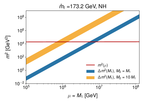
The results of the analysis are shown in Figs. 3, 4 for the case of normal neutrino mass hierarchy and . Fig. 3 shows (red line) vs. for degenerate states (blue band) and for (orange band). Eqn. (49a) is satisfied in the region where the bands overlap with the RGE curve: for the degenerate case we find161616Note that numerical subtleties of scanning parameter space using the Casas-Ibarra parameterization are known, see Ref. Casas:2010wm for a discussion. Exceptional parameter space can possibly exist outside the results shown, which are inferred from the numerical procedure above. The shown regions are expected to determine the bulk of the allowed parameter space.
| (50) | ||||||
while for lower values of are allowed. For the benchmark the viable mass region is
| (51) | ||||||
and intermediate values are possible for . Notably, has negligible dependence on both and . Therefore the range
| (52) |
is a general prediction of the neutrino option. Specific assumptions about the neutrino mass ordering and refine this range as detailed in Figure 6.
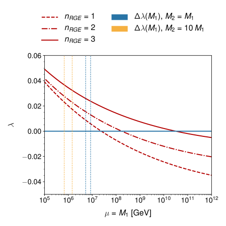
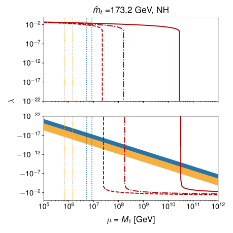
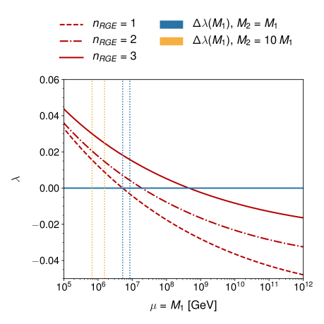
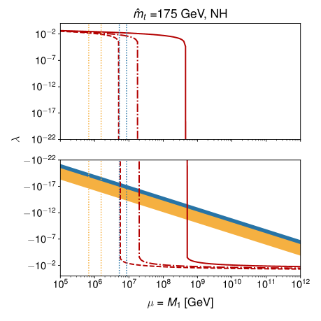
Fig. 4 shows vs , both in linear (left) and log scale (right). For reference, the regions in Eqns. (50), (51) are marked with blue and orange dotted vertical lines. Within these energy windows the threshold correction is always negative and very small, while the SM running curve is positive and . For the neutrino option to be realized it is then necessary that
| (53) |
4.3 Varying and other benchmark assumptions
Assuming an inverted neutrino mass hierarchy and taking different values of the top quark mass leads to qualitatively similar figures and has a modest impact on the numerical results. The main conclusions, i.e. the identification of the mass range in Eq. (52) and the necessity of a bare term in the Lagrangian, are general and emerge in all the benchmarks considered.
Note that the 3-loop RGE accuracy is crucial for establishing the condition as, for instance, an analysis restricted to does admit solutions of Eqns. (49) with Brivio:2017dfq . This is shown explicitly in Fig. 5, that reports the matching results for the parameter obtained with GeV. In this case, the dashed curve matches directly the threshold corrections band in the region where Eqn. (49a) is satisfied. This is consistent with what was observed in Ref. Brivio:2017dfq .
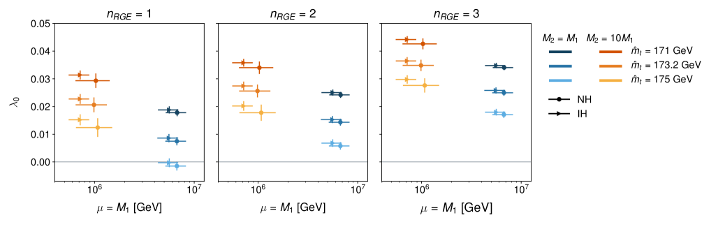
The values of (, ) where the neutrino option can be realized for each of the setups considered are summarized in Fig. 6. Varying either or mainly impacts , with larger and smaller giving a smoother running curve and consequently requiring larger values of in the matching. Choosing the inverse neutrino mass hierarchy rigidly results in slightly lower and slightly larger . This is easily understood as follows: in the IH case the neutrino masses are larger, which leads to larger (Eqn. (14)). The matching relation in Eqn. (49a) selects then a lower region compared to the NH case. Because is larger there, this has the indirect consequence of requiring a larger . Finally, the threshold correction is very sensitive to the relative size of the Majorana masses (see Fig. 2). Larger lead to lower being selected and, by the argument above, this indirectly requires larger . This explains the relative position of the blue and orange crosses in Fig. 6. The correction does not play any significant role in the numerical analysis as it is always for all the setups considered.
5 UV embeddings
The numerical results of Section 4 (see also Ref. Brivio:2017dfq ; Brdar:2018vjq ) show that a threshold matching defining a boundary condition for in the seesaw model can be consistent with the lower scale Higgs mass measured experimentally. This conclusion is robust against using in the results presented. As the coefficient of is dimensionful, this modifies the usual concerns of the Electroweak scale Hierarchy problem into an alternate framework.
For this framework to be embedded into a theoretically successful UV completion requires a UV scenario that can generate the Majorana scale used. This needs to occur in a manner that does not lead to other, larger, threshold matching conditions. Further, the threshold matching to the parameter, parametrically can be vanishingly small due to integrating out the Majorana Neutrino, as in order to separate the Majorana mass scale from the effective observed Electroweak scale. As a direct result, a small matching effect for can be subdominant to other UV boundary effects Brivio:2017dfq , or even a bare parameter, which is not forbidden by a symmetry. Explaining the origin of the required in a UV scenario would also advance the embedding of this theoretical framework in a more complete UV scenario.
5.1 The conformal UV embedding of the neutrino option of Ref. Brdar:2018vjq
Recently a UV framework for the Majorana scale generation was put forth in Ref. Brdar:2018vjq that addresses most of these theoretical challenges. The idea is to extend the SM with a set of scalar fields to generate the Majorana scale spontaneously by satisfying a Gildener-Weinberg Gildener:1976ih condition. The conformal UV completion of the neutrino option (hereafter the ) of Ref. Brdar:2018vjq is defined as
| (54) |
Here , are real singlet scalar fields, and has an odd charge under a symmetry Brdar:2018vjq .171717 It is interesting to note the consistency of the field content of this scenario with the the new minimal standard model of Ref. Davoudiasl:2004be . The latter does not examine a classically scale invariant starting point of parameter space, and is motivated out of minimality in addressing outstanding experimental deficiencies of the SM. The new minimal standard model does not utilize the neutrino option to generate the Higgs potential in the parameter space discussed in Ref. Davoudiasl:2004be , but can be considered to be a parameter space variant of the scenario considered here and proposed in Ref. Brdar:2018vjq . The running of the parameters leads to the condition
| (55) |
being satisfied, which leads to the spontaneous breaking of scale invariance once perturbative corrections are included in the Coleman-Weinberg (CW) potential Coleman:1973jx . is identified as the pseudo-Goldstone boson of broken scale invariance, the dilaton Salam:1969rq ; Salam:1970qk . also experiences a large breaking of its Goldstone nature by the coupling which has entries to the only other fields that are pure singlets, i.e. . The spontaneous breaking of scale invariance gives
| (56) |
and the mass spectrum is Gildener:1976ih ; Brdar:2018vjq
| (57) |
The interaction terms of the seesaw model can be written as in Eqn. (7) with all CP violating phases shifted to effective couplings and real diagonal entries in a mass matrix. This is conveniently done while by introducing states, defining a rotated diagonal coupling matrix . (The mass matrix in Eqn. (7) is in the diagonal mass basis with the prime superscripts dropped.) Using this notation the result in Eqn. (56) explicitly depends on the potential parameters through
| (58) |
and it is required that for physical solutions.The remaining contribution to the effective potential is given by Gildener:1976ih ; Brdar:2018vjq
| (59) |
and the relation between and is
| (60) |
An additional threshold contribution to of the form
| (61) |
is present, and the first term in this expression must dominate for the correct sign to be obtained for . The following set of consistency conditions are required to hold Brdar:2018vjq
| (62) |
The parameter space examined in Ref. Brdar:2018vjq is consistent with these conditions and such that
| (63) |
5.2 Extending the conformal neutrino option
Define a conformal transformation to be a smooth transformation of the metric
| (64) |
that preserves the causal structure of the theory. Further define the conformal weight of the scalar fields of the theory, collectively denoted , to be . A classically conformal UV embedding of the neutrino option requires some further extension due to the existence of gravity. First, this is because the scalar fields Klein-Gordon equations do not satisfy conformal invariance, until gravitational interactions are included. Second, the existence of the Planck scale itself is an explicit scale in the complete Lagrangian, calling into question the conformal starting point, and possibly leading to fine tuning.
Addressing the first challenge is straightforward. The leading interaction terms with gravity can be considered and fixed to specific classical values. Using a mostly positive metric convention the action is given by
Here is the Ricci scalar, is the reduced Planck mass, and . Note the scalar kinetic terms flip sign due to the adopted metric convention. At this stage the theory is necessarily non-renormalizable as the interaction terms represent an infinite tower of higher dimensional operators characterizing the interactions of the graviton with the dynamical field content. Eqn. (5.2) can be studied directly by expanding the metric around flat space in terms of the dynamical graviton field as which makes it clear that the Lagrangian term represents a the tower of higher dimensional operators. This set of interactions are dependent on the background field values and at large field values a large mixing of the scalar degrees of freedom with scalar modes of (non-canonically normalized) gravity results. The identification of the scale in the CW potential defined in field space, with particle masses leading to the threshold corrections of the neutrino option, ties together running in field space and the running in energy of the theory, that are formally distinct.
The effects of the non-minimal interactions with gravity are more easily studied by performing a transformation from the Jordan frame in Eqn. (5.2) to the Einstein frame of the theory. Taking and
| (66) |
as a further conformal transformation takes the theory to canonical form. The relevant results to study the higher dimensional operators generated already exist in the literature in Refs. Burgess:2010zq ; Bezrukov:2010jz . One finds the expression
| (67) | |||||
We are interested in the possible relation between the values of the parameters in the scalar potential in the CNO and the effects of the higher dimensional operators in Eqn. (67). Although expanding in small field values leads to a series of power corrections to potential terms, setting a lower bound on allowed coupling parameter space (when parameter tuning is avoided), we find the values of parameters examined in Ref. Brdar:2018vjq are still viable.
5.3 Possible fine tuning
Addressing the consistency of the Planck scale with a conformal embedding of the neutrino option is less straightforward. On the one hand, the required boundary values of the SM couplings at the Planck scale, including , are expected to be generated in a consistent UV theory which includes quantum gravity.181818The construction of such a theory is beyond the scope of this work, placing this paper in good company. The demand for such an embedding is reinforced by the fact that the SM interactions have Landau poles above the Planck scale. It is natural to speculate that a UV fixed point can appear in such a theory Weinberg1978 . If such a conformal field theory in the UV has an interacting fixed point, then the arguments of Ref. Tavares:2013dga imply that this scenario can be subject to fine tuning.
Here we review the relevant results of Ref. Tavares:2013dga to make the potential issue clear. The idea is that a contribution to the scalar two point function will be generated by the transition in the running behavior of the coupling constants of the theory. Consider the contribution to the scalar two point function determined by an approximately conformal field theory in position space following Ref. Tavares:2013dga
| (68) |
The scale is a non perturbative scale characterizing the changing in the running of the coupling constants from the IR free to UV fixed point behavior, that is assumed. This scale is not associated with a particle mass. Even so, the key point of Ref. Tavares:2013dga is that by assuming non-analytic dependence on the scale in the function , threshold matchings proportional to are generated for . We agree that the results of Ref. Tavares:2013dga follow from this assumed non-analytic dependence on . As the function is fundamentally non-perturbative it is not possible to draw strong conclusions about its analytic, or non-analytic form, without an explicit UV theory and non-perturbative study.
In the case at hand, we can examine if sensitivity to the scale for might already be present using perturbative methods. The presence of higher dimensional operators in Eqn. (67) indicates this theory is UV incomplete and the presence of the scale in Eqn (5.2) calls into question the starting assumption of conformal invariance. This theory does have a cut off scale associated with . The cut off scale is background field dependent Bezrukov:2010jz but given by Han:2004wt ; Burgess:2009ea ; Barbon:2009ya . The cut off scale comes from unitarity violation generated by the scattering diagram of the scalar multiplet coupled to gravity, while the singlet scalar fields do not introduce this cut off dependence Huggins:1987ea . Fundamentally this cut off scale stems from the interaction term . The conformal transformation in Eqn. (66) used to eliminate taking the theory to the Einstein frame results in a tower of higher dimensional operators effecting the CW potential as non-renormalizable classical potential terms.191919The effect of such operators on the effective potential is cogently discussed in Ref. Andreassen:2014eha . No contribution to is generated by such operators when expanding the effective potential through the particle thresholds leading to the SM. An inverse dependence on the scale is present breaking conformal symmetry explicitly.
In effective field theory, non-analytic behavior is usually associated with propagating long distance states of the theory, associated with the poles dictating the properties of the -matrix. Threshold matchings come about due to fixing that the IR limit of -matrix elements are reproduced when transitioning through a particle threshold. Non-perturbative matchings can be present, such as the effects of a multi-pole expansion due to underlying structure, which EFT can also be used to represent. Such effects introduce an inverse dependence on a heavy scale when integrated out, as the multi-pole expansion is a perturbative expansion in ratios of Compton wavelengths.202020See the SMEFT review Brivio:2017vri for more discussion.
The usual rules of EFT also dictate that a dimension two operator such as should be considered to have a dimensionful parameter . If this is the case, then this approach to the Hierarchy problem has severe fine tuning associated with it. Associating this cut off scale with physical particle masses, one does obtain large contributions to the operator . When not associating this cut off scale with physical particle masses, if a threshold contribution to is still generated, this would be consistent with the arguments in Ref. Tavares:2013dga . However, in this case, the cut-off scale is a sign that the effective field theory is smoothly transitioning from a linear SMEFT description to a non-linear EFT description Burgess:2014lza due to the Higgs field mixing with the scalar component of gravity. This mixing introduces non-linearities into the EFT description that require a different description of asymptotic states above and below the cut off scale. No particles are integrated out at this scale and the resulting background field dependent matching contributions across this threshold do not lead to a large shift in the Higgs mass at low field values. Extrapolating through this scale to large field values is subject to uncertainties due to introduced UV dependence, as the power counting of the EFT breaks down, but these effects do not necessarily generate a severe fine tuning of the Higgs mass parameter.
5.4 Comment on exceptional parameter space and Dark Matter
The set of consistency conditions given in Eqn. (5.1) can be satisfied if alternate parameter space is adopted than considered in Ref. Brdar:2018vjq . The field content and Lagrangian involving the scalar field coupled to the SM is the minimal singlet scalar field Dark Matter model Silveira:1985rk ; McDonald:1993ex ; Burgess:2000yq . It is interesting to lower the mass of the scalar to the scale for this reason using such alternate parameter space. The model parameter space with scale exotic scalar states can potentially provide a successful Dark Matter candidate. Viable parameter space for this model’s Dark Matter candidate has recently been highly constrained, see Refs. Cline:2013gha ; Athron:2017kgt ; Athron:2018ipf . The remaining viable parameter space can be consistent with Eqn. (5.1) at the cost of introducing small, technically natural, scalar couplings. In particular, the allowed resonance region of parameter space where can be chosen consistent with the constraints in Refs. Cline:2013gha ; Athron:2017kgt ; Athron:2018ipf while a "FIMP" scenario Hall:2009bx is present leading to a successful Dark matter relic density satisfying Bernal:2017kxu
| (69) |
In addition, as the scalar is a pseudo-Goldstone boson, ; a scattering channel is always kinematically open that depletes the relic abundance of . A straightforward calculation yields
| (70) |
For the exceptional parameter space to be viable, it is also necessary that additional Gildener-Weinberg Gildener:1976ih conditions discussed in Ref. Brdar:2018vjq must not be satisfied, to avoid spontaneously breaking scale invariance at scales other than . Finally, due to the presence of the scalar , and the self interactions of the field, the viability of the model is dependent on a nontrivial thermal history and also the balance of freeze-in and freeze out effects. We leave a detailed investigation of this possibility to a future publication.
6 Conclusions
In this paper, we have examined the neutrino option, where the Electroweak scale is generated simultaneously with neutrino masses. We have examined the numerical consistency of this scenario using one, two and three loop RGE equations for the SM, and one loop running of the Weinberg operator. We have developed a consistent NLO framework for such studies by determining the full set of () one loop corrections to the leading tree level matching. We have identified the requirement of a parameter at the matching scale and confirmed previous results that indicate that this scenario predicts Majorana states around the scales . We have also extended the conformal neutrino option scenario of Brdar et.al. Brdar:2018vjq to include the leading couplings to gravity. The conformal neutrino option necessarily includes a cut off scale due to scalar-graviton mixing. Nevertheless, we have also argued that this cut off scale does not result in a large fine tuning unless it is an indication of a UV-completion with Planck scale states, and in addition this cut off scale can be directly interpretted as a sign of a transition to a non-linear EFT set up around the Planck scale with no new states. It is far from obvious that calculable Planck scale threshold corrections to the Higgs mass can be demonstrated in this case. Overall, our results strongly support further investigations of the neutrino option and its conformal UV embedding being pursued.
Extensions to the Standard Model motivated out of the experimental requirement of neutrino mass generation remarkably remain an option to address the Hierarchy problem.
Acknowledgements.
MT and IB acknowledge generous support from the Villum Fonden and partial support by the Danish National Research Foundation (DNRF91) through the Discovery centre. We thank E. Bjerrum-Bohr, J. Bourjaily, J. Cline, A. Denner, W. Goldberger, H. Haber, A. Manohar, H. Murayama, S. Patil, P. Perez, S. Petcov, W. Skiba and J. Valle for useful discussions and comments.Appendix A Evaluating correlation functions in alternate Seesaw model formulations
Evaluating correlation functions when examining the neutrino option can be subtle due to the presence of a Majorana field. Feynman rules for Majorana particles exist in Ref. Denner:1992vza ; Denner:1992me ; Dreiner:2008tw , but subtleties can still remain, as we illustrate in this Appendix. Consider evaluating a vacuum expectation value of a correlation function using Wick’s theorem PhysRev.80.268 and comparing the results using the Lagrangians , . The interaction terms of , are classically identical,
Now consider evaluating using . Wick’s theorem gives
| (71) | |||||
Due to the presence of a Majorana field, one can use the transformation
| (72) |
before the contractions in Wick’s theorem are evaluated when considering the "self square" interaction terms , , also present in the time-ordered exponential. These transformations follow from transposing the interaction Lagrangian, and the Fermi-statistics of the fermionic field operators. Transposition of the Lagrangian is justified as the individual Lagrangian terms are invariant under the (compact Euclideanized ) Lorentz group, and the global . Although this transformation still allows the Majorana field to be contracted defining a two point function, as the correlation functions
no additional contribution to the sum of the time ordered product in Wick’s theorem results. These allowed transformations do lead to further contractions when considering other matrix elements, such as the three point and four point functions evaluated in this work, when using . A careful use of the Feynman rules of Refs. Denner:1992vza ; Denner:1992me still evaluates the correlation function in each case only using non-zero correlation functions , .
On the other hand, using and neglecting such "self square" interaction terms, directly gives
| (73) |
In this case, the "self square" of the manifestly charge symmetric interaction Lagrangian terms include
| (74) |
Using the charge conjugation identities, transposing the total Lagrangian, and Fermi-statistics gives
Using a manifestly charge symmetric interaction Lagrangian results in the additional contributions of this form, due to these allowed manipulations when evaluating the Wick expansion. An additional overall factor of two results evaluating , which brings the results obtained using , into agreement. A sign of the need to perform transformations of this form in evaluating the Wick expansion is the presence of non-zero contributions
| (75) |
These terms do not have a simple expression in terms of a charge conjugation matrix and gamma matrices, but indicate a transposition is required to evaluate the spin sum in some terms in the Wick expansion. On the other hand, when considering the three point function, the presence of the and fields leads to a direct evaluation of the Wick expansion in the formulation. Judiciously utilizing the transposition transformations can simplify various calculations when using or .
References
- (1) V. Brdar, Y. Emonds, A. J. Helmboldt, and M. Lindner, The Conformal UV Completion of the Neutrino Option, arXiv:1807.11490.
- (2) P. Minkowski, at a Rate of One Out of Muon Decays?, Phys. Lett. B67 (1977) 421–428.
- (3) M. Gell-Mann, P. Ramond, and R. Slansky, Complex Spinors and Unified Theories, Conf. Proc. C790927 (1979) 315–321, [arXiv:1306.4669].
- (4) R. N. Mohapatra and G. Senjanovic, Neutrino Mass and Spontaneous Parity Violation, Phys. Rev. Lett. 44 (1980) 912.
- (5) T. Yanagida, Horizontal Symmetry and Masses of Neutrinos, Prog. Theor. Phys. 64 (1980) 1103.
- (6) J. Schechter and J. W. F. Valle, Neutrino Masses in SU(2) x U(1) Theories, Phys. Rev. D22 (1980) 2227.
- (7) F. Vissani, Do experiments suggest a hierarchy problem?, Phys. Rev. D57 (1998) 7027–7030, [hep-ph/9709409].
- (8) I. Brivio and M. Trott, Radiatively Generating the Higgs Potential and Electroweak Scale via the Seesaw Mechanism, Phys. Rev. Lett. 119 (2017), no. 14 141801, [arXiv:1703.10924].
- (9) A. de Gouvea, J. Herrero-Garcia, and A. Kobach, Neutrino Masses, Grand Unification, and Baryon Number Violation, Phys. Rev. D90 (2014), no. 1 016011, [arXiv:1404.4057].
- (10) A. Kobach, Baryon Number, Lepton Number, and Operator Dimension in the Standard Model, Phys. Lett. B758 (2016) 455–457, [arXiv:1604.05726].
- (11) R. N. Mohapatra, Mechanism for Understanding Small Neutrino Mass in Superstring Theories, Phys. Rev. Lett. 56 (1986) 561–563.
- (12) R. N. Mohapatra and J. W. F. Valle, Neutrino Mass and Baryon Number Nonconservation in Superstring Models, Phys. Rev. D34 (1986) 1642. [,235(1986)].
- (13) J. Bernabeu, A. Santamaria, J. Vidal, A. Mendez, and J. W. F. Valle, Lepton Flavor Nonconservation at High-Energies in a Superstring Inspired Standard Model, Phys. Lett. B187 (1987) 303–308.
- (14) H. Davoudiasl and I. M. Lewis, Right-Handed Neutrinos as the Origin of the Electroweak Scale, Phys. Rev. D90 (2014), no. 3 033003, [arXiv:1404.6260].
- (15) J. A. Casas, V. Di Clemente, and M. Quiros, The Effective potential in the presence of several mass scales, Nucl. Phys. B553 (1999) 511–530, [hep-ph/9809275].
- (16) J. A. Casas, V. Di Clemente, A. Ibarra, and M. Quiros, Massive neutrinos and the Higgs mass window, Phys. Rev. D62 (2000) 053005, [hep-ph/9904295].
- (17) G. Bambhaniya, P. Bhupal Dev, S. Goswami, S. Khan, and W. Rodejohann, Naturalness, Vacuum Stability and Leptogenesis in the Minimal Seesaw Model, Phys. Rev. D95 (2017), no. 9 095016, [arXiv:1611.03827].
- (18) C. G. Callan, Jr., S. R. Coleman, and R. Jackiw, A New improved energy - momentum tensor, Annals Phys. 59 (1970) 42–73.
- (19) S. R. Coleman and R. Jackiw, Why dilatation generators do not generate dilatations?, Annals Phys. 67 (1971) 552–598.
- (20) W. A. Bardeen, On naturalness in the standard model, in Ontake Summer Institute on Particle Physics Ontake Mountain, Japan, August 27-September 2, 1995, 1995.
- (21) D. M. Capper and M. J. Duff, Trace anomalies in dimensional regularization, Nuovo Cim. A23 (1974) 173–183.
- (22) B. Bellazzini, C. Csaki, and J. Serra, Composite Higgses, Eur. Phys. J. C74 (2014), no. 5 2766, [arXiv:1401.2457].
- (23) W. Buchmüller and D. Wyler, Effective Lagrangian Analysis of New Interactions and Flavor Conservation, Nucl.Phys. B268 (1986) 621–653.
- (24) B. Grzadkowski, M. Iskrzynski, M. Misiak, and J. Rosiek, Dimension-Six Terms in the Standard Model Lagrangian, JHEP 1010 (2010) 085, [arXiv:1008.4884].
- (25) I. Brivio and M. Trott, The Standard Model as an Effective Field Theory, arXiv:1706.08945.
- (26) S. Weinberg, Baryon and Lepton Nonconserving Processes, Phys.Rev.Lett. 43 (1979) 1566–1570.
- (27) F. Wilczek and A. Zee, Operator Analysis of Nucleon Decay, Phys. Rev. Lett. 43 (1979) 1571–1573.
- (28) A. Broncano, M. B. Gavela, and E. E. Jenkins, The Effective Lagrangian for the seesaw model of neutrino mass and leptogenesis, Phys. Lett. B552 (2003) 177–184, [hep-ph/0210271]. [Erratum: Phys. Lett.B636,332(2006)].
- (29) G. Elgaard-Clausen and M. Trott, On expansions in neutrino effective field theory, JHEP 11 (2017) 088, [arXiv:1703.04415].
- (30) E. Majorana, Teoria simmetrica dell’elettrone e del positrone, Nuovo Cim. 14 (1937) 171–184.
- (31) S. M. Bilenky, J. Hosek, and S. T. Petcov, On Oscillations of Neutrinos with Dirac and Majorana Masses, Phys. Lett. 94B (1980) 495–498.
- (32) B. Pontecorvo, Mesonium and anti-mesonium, Sov. Phys. JETP 6 (1957) 429. [Zh. Eksp. Teor. Fiz.33,549(1957)].
- (33) Z. Maki, M. Nakagawa, and S. Sakata, Remarks on the unified model of elementary particles, Prog. Theor. Phys. 28 (1962) 870–880.
- (34) M. C. Gonzalez-Garcia, M. Maltoni, and T. Schwetz, Updated fit to three neutrino mixing: status of leptonic CP violation, JHEP 11 (2014) 052, [arXiv:1409.5439].
- (35) I. Esteban, M. C. Gonzalez-Garcia, M. Maltoni, I. Martinez-Soler, and T. Schwetz, Updated fit to three neutrino mixing: exploring the accelerator-reactor complementarity, JHEP 01 (2017) 087, [arXiv:1611.01514].
- (36) J. A. Casas and A. Ibarra, Oscillating neutrinos and muon —> e, gamma, Nucl. Phys. B618 (2001) 171–204, [hep-ph/0103065].
- (37) A. Ibarra, E. Molinaro, and S. T. Petcov, Low Energy Signatures of the TeV Scale See-Saw Mechanism, Phys. Rev. D84 (2011) 013005, [arXiv:1103.6217].
- (38) W. Grimus and H. Neufeld, Radiative Neutrino Masses in an SU(2) X U(1) Model, Nucl. Phys. B325 (1989) 18–32.
- (39) W. Grimus and L. Lavoura, One-loop corrections to the seesaw mechanism in the multi-Higgs-doublet standard model, Phys. Lett. B546 (2002) 86–95, [hep-ph/0207229].
- (40) P. S. B. Dev and A. Pilaftsis, Minimal Radiative Neutrino Mass Mechanism for Inverse Seesaw Models, Phys. Rev. D86 (2012) 113001, [arXiv:1209.4051].
- (41) E. Fernandez-Martinez, J. Hernandez-Garcia, J. Lopez-Pavon, and M. Lucente, Loop level constraints on Seesaw neutrino mixing, JHEP 10 (2015) 130, [arXiv:1508.03051].
- (42) D. Buttazzo, G. Degrassi, P. P. Giardino, G. F. Giudice, F. Sala, A. Salvio, and A. Strumia, Investigating the near-criticality of the Higgs boson, JHEP 12 (2013) 089, [arXiv:1307.3536].
- (43) K. S. Babu, C. N. Leung, and J. T. Pantaleone, Renormalization of the neutrino mass operator, Phys. Lett. B319 (1993) 191–198, [hep-ph/9309223].
- (44) S. Antusch, M. Drees, J. Kersten, M. Lindner, and M. Ratz, Neutrino mass operator renormalization revisited, Phys. Lett. B519 (2001) 238–242, [hep-ph/0108005].
- (45) J. A. Casas, J. R. Espinosa, A. Ibarra, and I. Navarro, General RG equations for physical neutrino parameters and their phenomenological implications, Nucl. Phys. B573 (2000) 652–684, [hep-ph/9910420].
- (46) A. Pilaftsis and T. E. J. Underwood, Resonant leptogenesis, Nucl. Phys. B692 (2004) 303–345, [hep-ph/0309342].
- (47) J. A. Casas, J. M. Moreno, N. Rius, R. Ruiz de Austri, and B. Zaldivar, Fair scans of the seesaw. Consequences for predictions on LFV processes, JHEP 03 (2011) 034, [arXiv:1010.5751].
- (48) E. Gildener and S. Weinberg, Symmetry Breaking and Scalar Bosons, Phys. Rev. D13 (1976) 3333.
- (49) H. Davoudiasl, R. Kitano, T. Li, and H. Murayama, The New minimal standard model, Phys. Lett. B609 (2005) 117–123, [hep-ph/0405097].
- (50) S. R. Coleman and E. J. Weinberg, Radiative Corrections as the Origin of Spontaneous Symmetry Breaking, Phys. Rev. D7 (1973) 1888–1910.
- (51) A. Salam and J. A. Strathdee, Nonlinear realizations. 1: The Role of Goldstone bosons, Phys. Rev. 184 (1969) 1750–1759.
- (52) A. Salam and J. A. Strathdee, Nonlinear realizations. 2. Conformal symmetry, Phys. Rev. 184 (1969) 1760–1768.
- (53) C. P. Burgess, H. M. Lee, and M. Trott, Comment on Higgs Inflation and Naturalness, JHEP 07 (2010) 007, [arXiv:1002.2730].
- (54) F. Bezrukov, A. Magnin, M. Shaposhnikov, and S. Sibiryakov, Higgs inflation: consistency and generalisations, JHEP 01 (2011) 016, [arXiv:1008.5157].
- (55) S. Weinberg, Critical Phenomena for Field Theorists, pp. 1–52. Springer US, Boston, MA, 1978.
- (56) G. Marques Tavares, M. Schmaltz, and W. Skiba, Higgs mass naturalness and scale invariance in the UV, Phys. Rev. D89 (2014), no. 1 015009, [arXiv:1308.0025].
- (57) T. Han and S. Willenbrock, Scale of quantum gravity, Phys. Lett. B616 (2005) 215–220, [hep-ph/0404182].
- (58) C. P. Burgess, H. M. Lee, and M. Trott, Power-counting and the Validity of the Classical Approximation During Inflation, JHEP 09 (2009) 103, [arXiv:0902.4465].
- (59) J. L. F. Barbon and J. R. Espinosa, On the Naturalness of Higgs Inflation, Phys. Rev. D79 (2009) 081302, [arXiv:0903.0355].
- (60) S. R. Huggins and D. J. Toms, One Graviton Exchange Interaction of Nonminimally Coupled Scalar Fields, Class. Quant. Grav. 4 (1987) 1509.
- (61) A. Andreassen, W. Frost, and M. D. Schwartz, Consistent Use of Effective Potentials, Phys. Rev. D91 (2015), no. 1 016009, [arXiv:1408.0287].
- (62) C. P. Burgess, S. P. Patil, and M. Trott, On the Predictiveness of Single-Field Inflationary Models, JHEP 06 (2014) 010, [arXiv:1402.1476].
- (63) V. Silveira and A. Zee, Scalar phantoms, Phys. Lett. 161B (1985) 136–140.
- (64) J. McDonald, Gauge singlet scalars as cold dark matter, Phys. Rev. D50 (1994) 3637–3649, [hep-ph/0702143].
- (65) C. P. Burgess, M. Pospelov, and T. ter Veldhuis, The Minimal model of nonbaryonic dark matter: A Singlet scalar, Nucl. Phys. B619 (2001) 709–728, [hep-ph/0011335].
- (66) J. M. Cline, K. Kainulainen, P. Scott, and C. Weniger, Update on scalar singlet dark matter, Phys. Rev. D88 (2013) 055025, [arXiv:1306.4710]. [Erratum: Phys. Rev.D92,no.3,039906(2015)].
- (67) GAMBIT Collaboration, P. Athron et al., Status of the scalar singlet dark matter model, Eur. Phys. J. C77 (2017), no. 8 568, [arXiv:1705.07931].
- (68) P. Athron, J. M. Cornell, F. Kahlhoefer, J. Mckay, P. Scott, and S. Wild, Impact of vacuum stability, perturbativity and XENON1T on global fits of and scalar singlet dark matter, arXiv:1806.11281.
- (69) L. J. Hall, K. Jedamzik, J. March-Russell, and S. M. West, Freeze-In Production of FIMP Dark Matter, JHEP 03 (2010) 080, [arXiv:0911.1120].
- (70) N. Bernal, M. Heikinheimo, T. Tenkanen, K. Tuominen, and V. Vaskonen, The Dawn of FIMP Dark Matter: A Review of Models and Constraints, Int. J. Mod. Phys. A32 (2017), no. 27 1730023, [arXiv:1706.07442].
- (71) A. Denner, H. Eck, O. Hahn, and J. Kublbeck, Feynman rules for fermion number violating interactions, Nucl. Phys. B387 (1992) 467–481.
- (72) A. Denner, H. Eck, O. Hahn, and J. Kublbeck, Compact Feynman rules for Majorana fermions, Phys. Lett. B291 (1992) 278–280.
- (73) H. K. Dreiner, H. E. Haber, and S. P. Martin, Two-component spinor techniques and Feynman rules for quantum field theory and supersymmetry, Phys. Rept. 494 (2010) 1–196, [arXiv:0812.1594].
- (74) G. C. Wick, The Evaluation of the Collision Matrix, Phys. Rev. 80 (1950) 268–272. [,592(1950)].