The Great Wall of SDSS galaxies

Abstract

An enhancement in the number of galaxies as function of the redshift is visible on the SDSS Photometric Catalogue DR 12 at z=0.383. This over-density of galaxies is named the Great Wall. This variable number of galaxies as a function of the redshift can be explained in the framework of the luminosity function for galaxies. The differential of the luminosity distance in respect to the redshift is evaluated in the framework of the LCDM cosmology.

Keywords: galaxy groups, clusters, and superclusters; large scale structure of the Universe Cosmology

1 Introduction

We review some early works on the ” CfA2 Great Wall”, which is the name that was introduced by [1] to classify an enhancement in the number of galaxies as a function of the redshift that is visible in the Center for Astrophysics (CfA) redshift survey [2]. The evaluation of the two point correlation function was done by [3] on the three slices of the CfA redshift survey. A careful analysis was performed on Sloan Digital Sky Survey (SDSS) DR4 galaxies by [4] : the great wall was detected in the range $0.07<z<0.09$. The substructures, the morphology and the galaxy contents were analyzed by [5, 6] and the luminosities and masses of galaxies were discussed in the framework of SDSS-III’s Baryon Oscillation Spectroscopic Survey (BOSS) [7]. The theoretical explanations for the Great Wall include an analysis of the peculiar velocities, see [8, 9], the nonlinear fields of the Zel’dovich approximation, see [10, 11, 12], and the cosmology of the Great Attractor, see [13]. The layout of the rest of this paper is as follows. In Section 2, we introduce the LCDM cosmology and the luminosity function for galaxies. In Section 3, we introduce the adopted catalog for galaxies and the theoretical basis of the maximum for galaxies as function of the redshift.

2 Preliminaries

This section introduces an approximate luminosity distance as a function of the redshift in LCDM and derives the connected differential. The Schechter luminosity function for galaxies is reviewed.

2.1 Adopted cosmology

Some useful formulae in $\Lambda$CDM cosmology can be expressed in terms of a Padé approximant. The basic parameters are: the Hubble constant, $H_{0}$, expressed in $\mathrm{km\,s^{-1}\,Mpc^{-1}}$, the velocity of light, $c$, expressed in $\mathrm{km\,s^{-1}}$, and the three numbers $\Omega_{\rm M}$, $\Omega_{K}$, and $\Omega_{\Lambda}$, see [14] for more details. In the case of the Union 2.1 compilation, see [15], the parameters are $H_{0}=69.81\mathrm{km\,s^{-1}\,Mpc^{-1}}$, $\Omega_{\rm M}=0.239$ and $\Omega_{\Lambda}=0.651$. To have the luminosity distance, $D_{L}(z;H_{0},c,\Omega_{\rm M},\Omega_{\Lambda})$, as a function of the redshift only, we apply the minimax rational approximation, which is characterized by the two parameters $p$ and $q$. We find a simplified expression for the luminosity distance, $D_{L,6,2}$, when $p=6$ and $q=2$

$$D_{L,6,2}=\frac{ND}{0.284483+0.153266\,z+0.0681615\,{z}^{2}}$$ (1)

$$\quad for\quad 0.001<z<4\quad,$$

where

$$ND=-0.0017+1221.80\,z+1592.35\,{z}^{2}+504.386\,{z}^{3}$$

$$+85.8574\,{z}^{4}+0.41684\,{z}^{5}+0.186189\,{z}^{6}\quad,$$ (2)

The inverse of the above function, i.e. the redshift $z_{6,2}$ as function of the luminosity distance, is

$$z_{6,2}=3.3754\,10^{-5}D_{{L}}-0.46438+{2.1625\times 10^{-14}}\times$$

$$\,\sqrt{2.4363\,10^{18}{D_{{L}}}^{2}+{3.9538\times 10^{23}}\,D_{{L}}+{4.6114\times 10^{26}}}\quad.$$ (3)

2.2 Luminosity function for galaxies

We used the Schechter function, see [16], as a luminosity function (LF) for galaxies

$$\Phi(L)dL=(\frac{\Phi^{*}}{L^{*}})(\frac{L}{L^{*}})^{\alpha}\exp\bigl{(}{-\frac{L}{L^{*}}}\bigr{)}dL\quad,$$ (4)

here $\alpha$ sets the slope for low values of luminosity, $L$, $L^{*}$ is the characteristic luminosity and $\Phi^{*}$ is the normalisation. The equivalent distribution in absolute magnitude is

$$\Phi(M)dM=0.921\Phi^{*}10^{0.4(\alpha+1)(M^{*}-M)}\exp\bigl{(}{-10^{0.4(M^{*}-M)}}\bigr{)}dM\quad,$$ (5)

where $M^{*}$ is the characteristic magnitude as derived from the data. The scaling with $h$ is $M^{*}-5\log_{10}h$ and $\Phi^{*}~{}h^{3}~{}[Mpc^{-3}]$.

3 The photometric maximum

This section models the Great Wall that is visible on the SDSS Photometric Catalogue DR 12. It also evaluates the theoretical number of galaxies as a function of the redshift.

3.1 The SDSS data

We processed the SDSS Photometric Catalogue DR 12, see [17], which contains 10450256 galaxies (elliptical + spiral) with redshift. In the following we will use the generic term galaxies without distinction between the two types, elliptical and spiral. The number of galaxies for an area in redshift of $0.025\times 0.025$ of the u-band is reported in Figure 1 as a contour plot and in Figure 2 as a cut along a line.

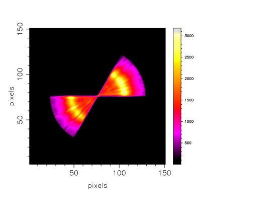
Figure 1: Contour for the number of galaxies (u-band) for areas of $0.025\times 0.025$.

Figure 2: The number of galaxies (u-band) along a line for areas of $0.025\times 0.025$.

3.2 The theory

The flux, $f$, is

$$f=\frac{L}{4\pi r^{2}}\quad,$$ (6)

where $r$ is the luminosity distance. The luminosity distance is

$$r=D_{L,6,2}\quad,$$ (7)

and the relationship between $dr$ and $dz$ is

$$dr=\frac{N}{D}dz\quad,$$ (8)

where

$$N=74813.67+10.9263\,{z}^{7}+49.05768\,{z}^{6}+2642.64259\,{z}^{5}$$

$$+16024.51314\,{z}^{4}+54307.16663\,{z}^{3}+127258.486\,{z}^{2}+$$

$$195005.8564\,z\quad,$$ (9)

and

$$D=\left({z}^{2}+2.248575472\,z+4.173664398\right)^{2}\quad.$$ (10)

The joint distribution in z and f for the number of galaxies is

$$\frac{dN}{d\Omega dzdf}=\frac{1}{4\pi}\int_{0}^{\infty}4\pi r^{2}dr\Phi(L;L^{*},\sigma)\delta\bigl{(}z-(z_{6,2})\bigr{)}\delta\bigl{(}f-\frac{L}{4\pi r^{2}}\bigr{)}\quad,$$ (11)

where $\delta$ is the Dirac delta function, $\Phi(L;L^{*},\sigma)$ has been defined in equation (4) and $z_{6,2}$ has been defined in equation (3). The explicit version is

$$\frac{dN}{d\Omega dzdf}=\frac{NN}{DD}\quad,$$ (12)

where

$$NN=644.3\,\left(z+1.058\right)^{4}\left(z-0.000001412\right)^{4}\times$$

$$\left({z}^{2}+4.889\,z+13.34\right)^{4}\left({z}^{2}-3.708\,z+464.6\right)^{4}\times$$

$${{\rm e}^{{\frac{{\it AA}}{{{\it BB}}^{2}{\it L^{*}}}}}}\left({\frac{CC}{{{\it BB}}^{2}{\it L^{*}}}}\right)^{\alpha}\times$$

$${\it\Phi^{*}}\,\left(z+0.5328\right)\left({z}^{2}+5.047\,z+7.9141\right)$$

$$\left({z}^{2}+0.7\,z+7.011\right)\left({z}^{2}-1.79\,z+231.58\right)\quad,$$ (13)

$$CC=f\left(z+1.058\right)^{2}\left(z-0.0000014124\right)^{2}\times$$

$$\left({z}^{2}+4.889\,z+13.343\right)^{2}\left({z}^{2}-3.708\,z+464.6\right)^{2}$$ (14)

$$DD=\left({z}^{2}+2.248\,z+4.173\right)^{6}{\it L^{*}}$$ (15)

$$AA=-93.76\,f{z}^{12}-419.8\,f{z}^{11}-86945.4\,f{z}^{10}$$

$$-701622.4\,f{z}^{9}-22679411\,f{z}^{8}-239083307\,f{z}^{7}$$

$$-1430432291\,f{z}^{6}-4912205831\,f{z}^{5}$$

$$+\left(4.540788\,\alpha\,{\it L^{*}}-10191896880\,f\right){z}^{4}+$$

$$\left(20.4206\,\alpha\,{\it L^{*}}-10524532830\,f\right){z}^{3}+\left(60.862\,\alpha\,{\it L^{*}}-4037704632\,f\right){z}^{2}$$

$$+\left(85.22\,\alpha\,{\it L^{*}}+11406.2\,f\right)z+79.098\,\alpha\,{\it L^{*}}-0.008055\,f\quad,$$ (16)

$$BB={z}^{2}+2.2485\,z+4.173\quad.$$ (17)

Figure 3 presents the number of galaxies that are observed in SDSS DR 12 as a function of the redshift for a given window in flux, in addition to the theoretical curve.

Figure 3: The galaxies of SDSS DR 12 (u-band) with $400\,L_{\odot}/Mpc^{2}\leq f\leq 5\,10^{7}\,L_{\odot}/Mpc^{2}$ are organized by frequency versus distance (empty circles) and the error bar is given by the square root of the frequency. The maximum frequency of the observed galaxies is at $z=0.38$. The full line is the theoretical curve that is generated by $\frac{dN}{d\Omega drdf}$ as given by the application of the Schechter LF, which is Equation (12), and the theoretical maximum is at $z=0.382$. The parameters are $L^{*}=2.038\,10^{10}L_{\odot}$ and $\alpha$ =-0.9  .

The theoretical number of galaxies is reported in Figure 4 as a function of the flux and redshift, and is reported in Figure 5 as a function of $\alpha$ and redshift.

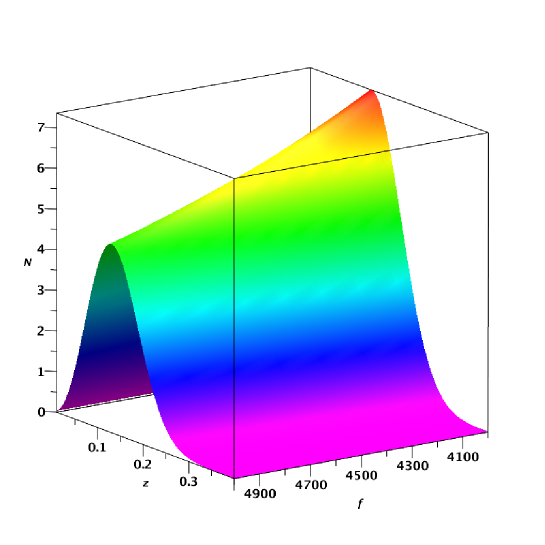
Figure 4: The theoretical number of galaxies divided by 1000 as a function of redshift and flux is expressed in $L_{\odot}/Mpc^{2}$. The parameters are $L^{*}=2.038\,10^{10}L_{\odot}$, $\alpha$ =-0.9 and $\frac{\Phi^{*}}{Mpc^{-3}}=0.038$  .

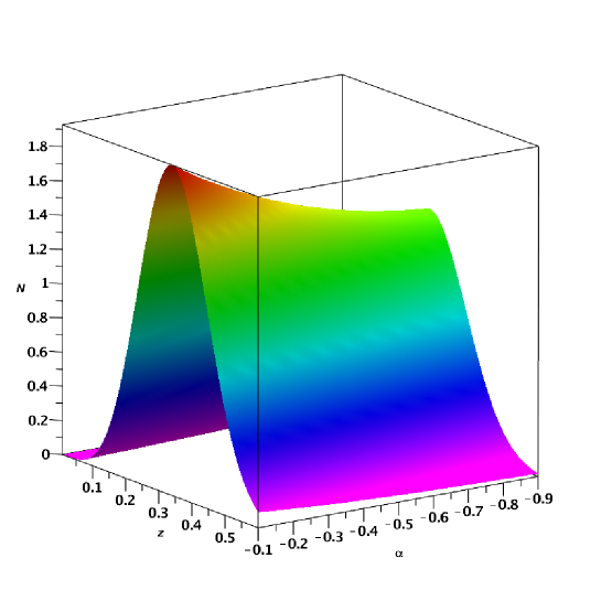
Figure 5: The theoretical number of galaxies divided by 100000 as a function of $\alpha$ and redshift when $L^{*}=2.038\,10^{10}L_{\odot}$, $f=1000\,L_{\odot}/Mpc^{2}$, and $\frac{\Phi^{*}}{Mpc^{-3}}=0.038$  .

The total number of galaxies comprised between a minimum value of flux, $f_{min}$, and a maximum value of flux $f_{max}$, for the Schechter LF can be computed through the integral

$$\frac{dN}{d\Omega dz}=\int_{f_{min}}^{f_{max}}\frac{NN}{DD}\,df\quad.$$ (18)

This integral has a complicated analytical solution in terms of the Whittaker function $M_{\kappa,\mu}\left(z\right)$, see [18]. Figure 6 reports all of the galaxies of SDSS DR12 and also the theoretical curve.

Figure 6: All of the galaxies of the SDSS DR12 catalog (u-band) are organized in frequencies versus spectroscopic redshift. The error bar is given by the square root of the frequency (Poisson distribution). The maximum frequency of all observed galaxies is at $z=0.383$. The full line is the theoretical curve generated by $\frac{dN}{d\Omega dz}(z)$ as given by the numerical integration of Eq. (18) with $L^{*}=2.038\,10^{10}L_{\odot}$, $\alpha=-0.9$ and $\frac{\Phi^{*}}{Mpc^{-3}}=0.038$  .

A theoretical surface/contour of the Great Wall is displayed in Figure 7

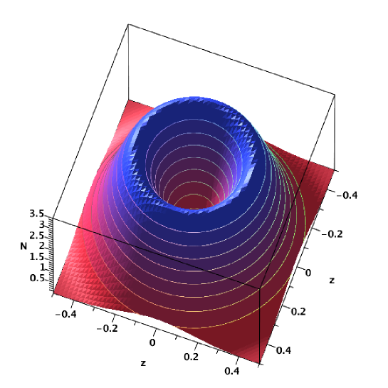
Figure 7: Theoretical surface/contour of the number of all the galaxies divided by 1000000 as a function of redshift. Parameters as in Figure 6.

4 Conclusions

$\Lambda$CDM cosmology

In this paper, we use the framework of $\Lambda$CDM cosmology with parameters $H_{0}=69.81\mathrm{km\,s^{-1}\,Mpc^{-1}}$, $\Omega_{\rm M}=0.239$ and $\Omega_{\Lambda}=0.651$. A relationship for the luminosity distance is derived using the method of the minimax approximation when $p=6$ and $q=2$, see equation (2.1). The inverse relationship, the redshift as function of the luminosity function is derived in equation (3).

The Great Wall

The enhancement in the number of galaxies as a function of the redshift for the SDSS Photometric Catalogue DR 12, which is at $z=0.383$, is here modeled by the theoretical equation (12) that is derived in the framework of the Schechter LF for galaxies and the $\Lambda$CDM cosmology . Figure 6 reports the observed maximum in the number of galaxies and also the theoretical curve. These results are in agreement with a catalog of photometric redshift of $\approx$ 3000000 SDSS DR8 galaxies made by [19] : their Figure 9 bottom reports that the count of elliptical galaxies has a peak at $z\approx 0.37$ when the spirals galaxies conversely peaks at $z\approx 0.08$.

References

• [1] Geller M J and Huchra J P 1989 Mapping the universe Science 246, 897
• [2] de Lapparent V, Geller M J and Huchra J P 1989 The luminosity function for the CfA redshift survey slices ApJ  343, 1
• [3] Ramella M, Geller M J and Huchra J P 1992 The distribution of galaxies within the ’Great Wall’ ApJ  384, 396
• [4] Deng X F, He J Z, He C G and et al 2007 The Sloan Great Wall from the SDSS Data Release 4 Acta Physica Polonica B 38, 219
• [5] Einasto M, Tago E, Saar E and et al 2010 The Sloan great wall. Rich clusters A&A  522 A92 (Preprint 1007.4492)
• [6] Einasto M, Liivamägi L J, Tempel E and et al 2011 The Sloan Great Wall. Morphology and Galaxy Content ApJ  736 51 (Preprint 1105.1632)
• [7] Einasto M, Lietzen H, Gramann M and et al 2017 BOSS Great Wall: morphology, luminosity, and mass A&A  603 A5 (Preprint 1703.08444)
• [8] dell’Antonio I P, Bothun G D and Geller M J 1996 Peculiar Velocities for Galaxies in the Great Wall.I.The Data AJ 112, 1759
• [9] dell’Antonio I P, Geller M J and Bothun G D 1996 Peculiar Velocities for Galaxies in the Great Wall.II.Analysis AJ 112, 1780
• [10] Zel’dovich Y B 1970 Gravitational instability: An approximate theory for large density perturbations. A&A  5, 84
• [11] Shandarin S F 2009 The origin of ‘Great Walls’ Journal of Cosmology and Astroparticle Physic 2 031 (Preprint 0812.4771)
• [12] Shandarin S F 2011 The multi-stream flows and the dynamics of the cosmic web Journal of Cosmology and Astroparticle Physic 5 015 (Preprint 1011.1924)
• [13] Valkenburg W and Bjælde O E 2012 Cosmology when living near the Great Attractor MNRAS  424, 495 (Preprint 1203.4567)
• [14] Zaninetti L 2016 Pade approximant and minimax rational approximation in standard cosmology Galaxies 4(1), 4 ISSN 2075-4434 URL http://www.mdpi.com/2075-4434/4/1/4
• [15] Suzuki N, Rubin D, Lidman C, Aldering G, Amanullah R, Barbary K and Barrientos L F 2012 The Hubble Space Telescope Cluster Supernova Survey. V. Improving the Dark-energy Constraints above z greater than 1 and Building an Early-type-hosted Supernova Sample ApJ  746 85
• [16] Schechter P 1976 An analytic expression for the luminosity function for galaxies. ApJ  203, 297
• [17] Alam S, Albareti F D, Allende Prieto C and et al 2015 The Eleventh and Twelfth Data Releases of the Sloan Digital Sky Survey: Final Data from SDSS-III ApJS 219 12 (Preprint 1501.00963)
• [18] Olver F W J e, Lozier D W e, Boisvert R F e and Clark C W e 2010 NIST handbook of mathematical functions. (Cambridge: Cambridge University Press. )
• [19] Paul N, Virag N and Shamir L 2018 A catalog of photometric redshift and the distribution of broad galaxy morphologies Galaxies 6(2)