SVD update methods for large matrices and applications

Abstract

We consider the problem of updating the SVD when augmenting a “tall thin” matrix, i.e., a rectangular matrix $A\in\mathbb{R}^{m\times n}$ with $m\gg n$. Supposing that an SVD of $A$ is already known, and given a matrix $B\in\mathbb{R}^{m\times n^{\prime}}$, we derive an efficient method to compute and efficiently store the SVD of the augmented matrix $[AB]\in\mathbb{R}^{m\times(n+n^{\prime})}$. This is an important tool for two types of applications: in the context of principal component analysis, the dominant left singular vectors provided by this decomposition form an orthonormal basis for the best linear subspace of a given dimension, while from the right singular vectors one can extract an orthonormal basis of the kernel of the matrix. We also describe two concrete applications of these concepts which motivated the development of our method and to which it is very well adapted.

1 Introduction

The singular value decomposition $A=U\Sigma V^{T}$ of a matrix $A\in\mathbb{R}^{m\times n}$ is a useful and important tool in many applications and there exist algorithms and even toolboxes to perform this task numerically. Indeed, the matrices $U$, $V$, obtained in the decomposition give valuable information about $A$ in a compressed way: the singular vectors, the columns of the matrix $U$, give best low dimensional approximations of the subspace generated by the columns of $A$, while the matrix $V$ reliably detects the kernel of the matrix $A$ and therefore is the method of choice for numerical rank detection, see [1, 2].

In many applications, specifically in video processing or in the multivariate versions of Prony’s method, the full matrix $A$ is not known from the beginning, but is built by successively adding columns or blocks of columns; these added blocks can correspond to new measurements or can just be determined by the algorithm itself. What these applications have in common is that the columns of the matrices are large, i.e., $m\gg n$. This calls for reliable and efficient update algorithms for a matrix whose SVD is already known. Such an algorithm, due to Businger [3], is described in [4], however this algorithm, more precisely its transposed version to add columns, then assumes that $m\leq n$ which means that it adds mostly redundant columns. In [5], Brand more recently gave a fast algorithm to update few dominant singular values of an augmented matrix which was used, for example, to perform background elimination in videos [6]. Brand’s method is based on an efficient way to perform rank $1$ modifications, see [5, Sections 3 and 4.1], hence it would proceed columnwise to add a full block. In this paper, we give an algorithm that adds the columns simultaneously to a “tall and thin” matrix, but always computes the full SVD in an efficient way, and point out the connections to PCA based video analysis and Prony’s method.

In the latter, the main numerical problem in the algorithms presented in [7, 8] is to determine reliably the nullspaces of sequences of matrices that are generated by successively adding blocks of columns. Adding these columns corresponds to extending a symmetric H–basis for an ideal, and treating them in a symmetric way and not attaching them in some order is of great importance for the numerical performance of such algorithms. In other words, we have to determine the nullspaces of sequences

$$B_{0},\quad[B_{0}\,B_{1}],\quad[B_{0}\,B_{1}\,B_{2}],\dots,$$

where, depending on the algorithm used, $B_{j}$ can be a single column or a block of several columns. Clearly, the rank of these matrices is increasing which is, however, not captured by a naive application of Matlab’s rank command to the augmented matrices. Since numerical rank computations are usually based on a singular value decomposition (SVD) of the matrix, we aim for a method which uses an already existing SVD of a given matrix $A_{k}$ to compute the SVD of the column augmented $A_{k+1}=[A_{k}\,B_{k}]$ in an efficient, numerically stable and reliable way.

Though the concrete method we develop and investigate here is new, the problem itself has been considered before. Indeed, Updating methods for rank revealing factorizations have been considered by Stewart [9] in a very similar context, namely for the MUSIC algorithm [10] that solves Prony’s problem in one variable in the context of multisource radar signal processing. Other approaches for updating SVD and QR algorithm can be found in [11] and [12], respectively. Incremental methods for dominant singular subspaces were also considered in [13], where only some dominant singular vectors were computed. In contrast to that, our approach aims to always compute the full thin SVD of the matrix which is especially needed for kernel computations.

The layout of the paper is as follows. In Section 2 we present our method to update the SVD and analyze its computational cost. Section 3 presents a corresponding thresholding strategy, which is designed ensure that increasing ranks are detected properly. Section 4 presents two applications for which the augmented SVD method is very well suited: to Principal Component Analysis of videos in Subsection 4.3 and to the already mentioned solution of Prony’s problem in several variables, see Subsection 4.4.

2 Updating decompositions – idea and details

We are considering processes that determine matrices $A_{k}\in\mathbb{R}^{d\times n_{k}}$, $k=1,2,\dots$, by the iterative block column extension

$$A_{k+1}=\left[A_{k}\,B_{k}\right],\qquad B_{k}\in\mathbb{R}^{d\times m_{k}},\qquad m_{k}:=n_{k+1}-n_{k},$$ (1)

where $n_{k}\leq d$, usually $n_{k}\ll d$, and want to compute a rank revealing decomposition or an SVD for $A_{k+1}$ in an efficient and numerically stable way from that of $A_{k}$.

We begin with the SVD and adapt an idea to our needs which is referenced in [4], as Businger’s method [3]. The exposition in [4], however, extends a matrix with more rows than columns by adding a further row and it is mentioned in passing that adding of columns can be done by transposition. Then, however, the matrix should have more columns than rows which is not the case in our situation. Nevertheless, the basic idea can be adapted.

To that end, we assume that we already computed a decomposition

$$A_{k}=U_{k}\Sigma_{k}V_{k}^{T},\qquad{\mathop{\rm rank\,}\nolimits}A_{k}=:r_{k}\leq n_{k}\leq d,$$ (2)

with orthogonal matrices

$$U_{k}\in\mathbb{R}^{d\times d},\qquad V_{k}\in\mathbb{R}^{n_{k}\times n_{k}},$$ (3)

and the diagonal matrix

$$\Sigma_{k}=\left[\begin{array}[]{cc}\Sigma_{k}^{\prime}&0_{r_{k}\times(n_{k}-r_{k})}\\ 0_{(d-r_{k})\times r_{k}}&0_{(d-r_{k})\times(n_{k}-r_{k})}\end{array}\right]\in\mathbb{R}^{d\times n_{k}},\qquad\Sigma_{k}^{\prime}\in\mathbb{R}^{r_{k}\times r_{k}},$$ (4)

where $\Sigma_{k}^{\prime}$ has strictly positive diagonal values.

Remark 2.1

Due to (3), the factorization is formally not a “slim” or “economic” decomposition of $A_{k}$. Such a decomposition would be of the form

$$A_{k}=U\Sigma V^{T},\qquad U\in\mathbb{R}^{d\times r_{k}},\,\Sigma\in\mathbb{R}^{r_{k}\times r_{k}},\,V\in\mathbb{R}^{r_{k}\times n_{k}},$$

with all diagonal elements of $\sigma$ being positive.

Note, however, that in (2) the last $d-r_{k}$ columns of $U$ and the last $n_{k}-r_{k}$ columns ov $V$ are irrelevant for the validity of the decomposition, hence it is not unique. We will later describe how to represent one such decomposition with a memory effort that only exceeds that of a thin representation by $r_{k}(r_{k}+n_{k})$ elements. This is negligible in the case when $d\gg n_{k}$ and has the advantage that we always compute a full orthonormal basis of the kernel of $A_{k}$, which was motivated by its importance for the Prony application.

In what follows, we first deduce the updating method in a general fashion and give the numerically efficient implementations of the crucial steps afterwards. To that end, we define in a straightforward way,

$$X:=U_{k}^{T}A_{k+1}\left[\begin{array}[]{cc}V_{k}&0\\ 0&I\end{array}\right]=U_{k}^{T}[A_{k}\,B_{k}]\left[\begin{array}[]{cc}V_{k}&0\\ 0&I\end{array}\right]=\left[\Sigma_{k}\,|\,U_{k}^{T}B_{k}\right]$$

and observe that

$$X=\left[\begin{array}[]{ccc}\Sigma_{k}^{\prime}&0&*\\ 0&0&*\end{array}\right]=\left[\begin{array}[]{ccc}\Sigma_{k}^{\prime}&*&0\\ 0&*&0\end{array}\right]\,P_{k}=:\left[\begin{array}[]{ccc}\Sigma_{k}^{\prime}&Y^{\prime}&0\\ 0&Y&0\end{array}\right]\,P_{k}$$ (5)

for the permutation matrix

$$P_{k}=\left[\begin{array}[]{ccc}I_{r_{k}}&0&0\\ 0&0&I_{n_{k}-r_{k}}\\ 0&I_{m_{k}}&0\end{array}\right]\in\mathbb{R}^{n_{k+1}\times n_{k+1}},$$

that permutes the last $n_{k+1}-r_{k}$ columns. Next, we apply a QR method with column pivoting on the matrix $Y\in\mathbb{R}^{(d-r_{k})\times m_{k}}$, finding a permutation $P\in\mathbb{R}^{m_{k}\times m_{k}}$ and a decomposition

$$Y=\widetilde{Q}\,\left[\begin{array}[]{c}\widetilde{R}\\ 0\end{array}\right]\,P,\qquad\widetilde{Q}\in\mathbb{R}^{(d-r_{k})\times(d-r_{k})},\quad\widetilde{R}\in\mathbb{R}^{m_{k}\times m_{k}},$$ (6)

where, as usually in rank revealing factorizations, column pivoting ensures that the entries of $\widetilde{R}=\left[\tilde{r}_{ij}:i,j=1,\dots,m_{k}\right]$ satisfy

$$|\tilde{r}_{11}|\geq\cdots\geq|\tilde{r}_{m_{k},m_{k}}|\qquad\text{and}\qquad|\tilde{r}_{jj}|\geq|\tilde{r}_{j\ell}|,\quad\ell\geq j,\,j=1,\dots,m_{k}.$$ (7)

Defining the orthogonal matrix

$$Q=\left[\begin{array}[]{cc}I_{r_{k}\times r_{k}}&0\\ 0&\widetilde{Q}\end{array}\right]\in\mathbb{R}^{d\times d},$$

the decomposition (6) yields that

$$Q^{T}\left[\begin{array}[]{c}Y^{\prime}\\ Y\end{array}\right]=\left[\begin{array}[]{c}Y^{\prime}\\ \widetilde{Q}^{T}Y\end{array}\right]=\left[\begin{array}[]{c}Y^{\prime}P^{T}\\ \widetilde{R}\\ 0\end{array}\right]P.$$ (8)

The computation of the matrix $\widetilde{R}$ from (6) is also the starting point for a thresholding algorithm to be described in the next section. Substituting (8) into (5) we then also get

$$Q^{T}X=\left[\begin{array}[]{ccc}\Sigma_{k}^{\prime}&Y^{\prime}P^{T}&0\\ 0&\widetilde{R}&0\\ 0&0&0\end{array}\right]\left[\begin{array}[]{ccc}I_{r_{k}}\\ &P\\ &&I_{n_{k}-r_{k}}\end{array}\right]P_{k}=\left[\begin{array}[]{ccc}\Sigma_{k}^{\prime}&Y^{\prime}P^{T}&0\\ 0&\widetilde{R}&0\\ 0&0&0\end{array}\right]P_{k}^{\prime}P_{k},$$ (9)

with the block diagonal permutation

$$P_{k}^{\prime}:=\left[\begin{array}[]{ccc}I_{r_{k}}&&\\ &P\\ &&I_{n_{k}-r_{k}}\end{array}\right]$$

that satisfies

$$P_{k}^{\prime}P_{k}=\left[\begin{array}[]{ccc}I&&\\ &P\\ &&I\end{array}\right]\left[\begin{array}[]{ccc}I&&\\ &&I\\ &I&\end{array}\right]=\left[\begin{array}[]{ccc}I&&\\ &&P\\ &I&\end{array}\right].$$

Therefore, using the abbreviation $p_{k}:=r_{k}+m_{k}$, $r_{k+1}\leq p_{k}\leq n_{k+1}$, we obtain another upper triangular matrix of relatively small size:

$$Q^{T}X(P_{k}^{\prime}P_{k})^{T}=\left[\begin{array}[]{ccc}\Sigma_{k}^{\prime}&Y^{\prime}P^{T}&0\\ 0&\widetilde{R}&0\\ 0&0&0\end{array}\right]=:\left[\begin{array}[]{cc}R_{k+1}&0\\ 0&0\end{array}\right],\qquad R_{k+1}\in\mathbb{R}^{p_{k}\times p_{k}}.$$ (10)

Next, we compute a singular value decomposition of $R_{k+1}$ as

$$R_{k+1}=\widetilde{U}\,\left[\begin{array}[]{cc}\Sigma_{k+1}^{\prime}&0\\ 0&0\end{array}\right]\widetilde{V}^{T},\qquad\qquad\widetilde{U},\widetilde{V}\in\mathbb{R}^{p_{k}\times p_{k}},\;\Sigma_{k+1}^{\prime}\in\mathbb{R}^{r_{k+1}\times r_{k+1}},$$ (11)

where $\Sigma_{k+1}^{\prime}$ has strictly positive singular values that can be controlled by means of the thresholding strategies in the next section. This also determines the rank $r_{k+1}$ of $A_{k+1}$.

These results can be recombined into an efficient SVD of the $d\times n_{k+1}$ matrix

$$Q^{T} X(P_{k}^{\prime}P_{k})^{T}$$

$$=\left[\begin{array}[]{cc}\widetilde{U}&0\\ 0&I_{d-p_{k}}\\ \end{array}\right]\left[\begin{array}[]{cc}\Sigma_{k+1}^{\prime}&0\\ 0&0_{(d-r_{k+1})\times(n_{k+1}-r_{k+1})}\end{array}\right]\left[\begin{array}[]{cc}\widetilde{V}^{T}&0\\ 0&I_{n_{k+1}-p_{k}}\end{array}\right].$$ (18)

Since $p_{k}=r_{k}+m_{k}\leq n_{k+1}$ with equality iff $r_{k}=n_{k}$, i.e., iff $A_{k}$ has full rank, we can always assume that

$$\widetilde{U},\widetilde{V}\in\mathbb{R}^{n_{k+1}\times n_{k+1}},$$

so that the storage requirement for these matrices is at most $n_{k+1}^{2}$. Note, however, that the matrices in (18) are now patterned in different ways and that only their overall dimensions coincide. Combining all decompositions, finally gives

$$A_{k+1}=U_{k}X\left[\begin{array}[]{cc}V_{k}^{T}&0\\ 0&I\end{array}\right]$$

$$= U_{k}Q\left[\begin{array}[]{cc}\widetilde{U}&0\\ 0&I\end{array}\right]\left[\begin{array}[]{cc}\Sigma_{k+1}^{\prime}&0\\ 0&0\end{array}\right]\left[\begin{array}[]{cc}\widetilde{V}^{T}&0\\ 0&I\end{array}\right]\,P_{k}^{\prime}P_{k}\,\left[\begin{array}[]{cc}V_{k}^{T}&0\\ 0&I\\ \end{array}\right]$$

$$=: U_{k+1}\Sigma_{k+1}V_{k+1}^{T},$$

with the update rules

$$U_{k+1} = U_{k}Q\left[\begin{array}[]{cc}\widetilde{U}&0\\ 0&I\end{array}\right],$$ (23)

$$V_{k+1} = \left[\begin{array}[]{cc}V_{k}&0\\ 0&I\end{array}\right](P_{k}^{\prime}P_{k})^{T}\left[\begin{array}[]{cc}\widetilde{V}&0\\ 0&I\end{array}\right].$$ (28)

The matrices appearing in (23) are all of dimension $d\times d$, the ones used in (28) of dimension $n_{k+1}\times n_{k+1}$.

Remark 2.2

The re-computation of all singular values in (11) is unavoidable since, for example the interlacing property of singular values of an augmented matrix tells us that usually all the singular values will change.

Remark 2.3

Businger’s method as described in [4] and also the efficient methods in [5] treat only the case of adding a single row to the matrix. In the algebraic applications, especially in the multivariate version of Prony’s method, however, it is important to treat the addition of several columns at the same time and treat these columns as symmetric as possible.

Since in the applications we consider, the dimension $d$ and therefore the size of $U_{k}\in\mathbb{R}^{d\times d}$ can be rather large, it is not reasonable to store $U_{k}$ in dense form. Normally, this is done by the aforementioned thin SVD with $U\in\mathbb{R}^{d\times r}$, $\Sigma\in\mathbb{R}^{r\times r}$ and $V\in\mathbb{R}^{r\times n}$, where $r$ is the rank of the matrix $A=U\Sigma V^{T}\in\mathbb{R}^{d\times n}$. The storage requirement for such representations is $dr+r^{2}+rn=r(r+d+n)$ and thus only linear in the dominant direction $d$.

To obtain a similar storage performance and be able to apply fast algorithms, we will store $U_{k}$ as a factorization by means of Householder vectors instead, cf. [2]. Recall that for a vector $y\in\mathbb{R}^{d}$ the Householder reflection matrix $H_{y}=I-2\frac{yy^{T}}{y^{T}y}$ is a symmetric orthogonal matrix that can be used for obtaining the QR factorization. Indeed, since the QR factorization of $Y$ has to annihilate a lot of numbers simultaneously in any step, it is reasonable to perform it by Householder reflections so that

$$Q=\prod_{j=1\uparrow p}(I-y_{j}y_{j}^{T})=:\left(I-y_{1}y_{1}^{T}\right)\cdots\left(I-y_{p}y_{p}^{T}\right),\qquad\|y_{j}\|_{2}=\sqrt{2},\quad j=1,\dots,p,$$ (29)

for some $p\in\mathbb{N}$. Note that we write the noncommutative matrix products in a left-to-right way which means that

$$Q^{T}=\left(I-y_{p}y_{p}^{T}\right)\cdots\left(I-y_{1}y_{1}^{T}\right)=:\prod_{j=p\downarrow 1}(I-y_{j}y_{j}^{T}),$$

which is slight unconventional but convenient.

Lemma 2.4

If $Q$ is the orthogonal matrix from the $QR$ factorization (8), then $p=r_{k+1}-r_{k}$.

Proof:   The decomposition (6) of $Y$ can be written as

$$\widetilde{Q}^{T}YP^{T}=\left[\begin{array}[]{cc}R^{\prime}&*\\ 0&0\end{array}\right],\qquad R^{\prime}\in\mathbb{R}^{p\times p},$$

if the column pivoting terminates after $p$ steps. Hence, by (10),

$$R_{k+1}=\left[\begin{array}[]{ccc}\Sigma_{k}^{\prime}&*&*\\ &R^{\prime}&*\\ &0&0\end{array}\right],$$

and therefore $r_{k+1}={\mathop{\rm rank\,}\nolimits}R_{k+1}=r_{k}+p$ since $r_{k}+p$ diagonal elements of the upper triangular matrix $R_{k+1}$ are nonzero. $\Box$

Since for any orthogonal matrix $U\in\mathbb{R}^{d\times d}$ one has

$$H_{y}U=(I-yy^{T})U=U-y(U^{T}y)^{T}=U\left(I-(U^{T}y)(U^{T}y)^{T}\right)=UH_{U^{T}y},$$

the matrix

$$Q\left[\begin{array}[]{cc}\widetilde{U}&0\\ 0&I\end{array}\right]=\left[\begin{array}[]{cc}\widetilde{U}&0\\ 0&I\end{array}\right]\,\prod_{j=1\uparrow{r_{k+1}-r_{k}}}(I-\tilde{y}_{j}\tilde{y}_{j}^{T})$$

from (23) can be represented by $\widetilde{U}\in\mathbb{R}^{n_{k+1}\times n_{k+1}}$ and the vectors

$$\tilde{y}_{j}:=\left[\begin{array}[]{cc}\widetilde{U}^{T}&0\\ 0&I\end{array}\right]y_{j},\qquad j=1,\dots,r_{k+1}-r_{k}.$$

Hence, if we assume that we already have computed a representation of the form

$$U_{k}=\left[\begin{array}[]{cc}\widetilde{U}_{k}&0\\ 0&I\end{array}\right]\prod_{j=1\uparrow r_{k}}(I-h_{j}h_{j}^{T}),$$ (30)

where we store the Householder vectors as columns of a matrix

$$H_{k}:=\left[h_{1},\dots,h_{r_{k}}\right]\in\mathbb{R}^{d\times r_{k}},$$ (31)

the update rule (23) becomes

$$U_{k+1} = U_{k}Q\left[\begin{array}[]{cc}\widetilde{U}&0\\ 0&I\\ \end{array}\right]$$

$$= \left[\begin{array}[]{cc}\widetilde{U}_{k}&0\\ 0&I\end{array}\right]\prod_{j=1\uparrow r_{k}}(I-h_{j}h_{j}^{T})\,\left[\begin{array}[]{cc}\widetilde{U}&0\\ 0&I\\ \end{array}\right]\prod_{j=1\uparrow r_{k+1}-r_{k}}(I-\tilde{y}_{j}\tilde{y}_{j}^{T})$$

$$= \left[\begin{array}[]{cc}\widetilde{U}_{k}&0\\ 0&I\\ \end{array}\right]\left[\begin{array}[]{cc}\widetilde{U}&0\\ 0&I\\ \end{array}\right]\prod_{j=1\uparrow r_{k}}(I-\tilde{h}_{j}\tilde{h}_{j}^{T})\prod_{j=1\uparrow r_{k+1}-r_{k}}(I-\tilde{y}_{j}\tilde{y}_{j}^{T})$$

$$= \left[\begin{array}[]{cc}\widetilde{U}_{k}&0\\ 0&I\\ \end{array}\right]\left[\begin{array}[]{cc}\widetilde{U}&0\\ 0&I\\ \end{array}\right]\prod_{j=1}^{r_{k+1}}(I-\tilde{h}_{j}\tilde{h}_{j}^{T}),$$

which can be represented by the matrix

$$\widetilde{U}_{k+1}=\left[\begin{array}[]{cc}\widetilde{U}_{k}&0\\ 0&I\\ \end{array}\right]\left[\begin{array}[]{cc}\widetilde{U}&0\\ 0&I\\ \end{array}\right]\in\mathbb{R}^{n_{k+1}\times n_{k+1}}$$ (36)

and the $r_{k+1}$ vectors

$$\tilde{h}_{j}=\left[\begin{array}[]{cc}\widetilde{U}^{T}&0\\ 0&I\end{array}\right]\,\left\{\begin{array}[]{ccl}h_{j},&&j=1,\dots,r_{k},\\ y_{j-r_{k}},&&j=r_{k}+1,\dots,r_{k+1},\end{array}\right.$$ (37)

or, in matrix notation,

$$H_{k+1}=\left[\begin{array}[]{cc}\widetilde{U}^{T}&0\\ 0&I\end{array}\right]\,\left[H_{k},\,y_{1},\dots,y_{r_{k+1}-r_{k}}\right].$$ (38)

The storage requirement for the matrix $H_{k+1}$ on level $k+1$ is therefore $n_{k+1}\,(d+n_{k+1})$ and the computational effort for the update step is $O(n_{k+1}^{3})$ for the matrix-matrix product in (36) plus $O(n_{k+1}^{2}r_{k+1})$ for the product in (37) since the last $d-n_{k+1}$ entries in each column of the product can simply be copied. Thus, we can estimate the computational effort by a total of $O\left(n_{k+1}^{2}(n_{k+1}+r_{k+1})\right)$.

Remark 2.5

Another advantage of storing the matrix $U_{k}$ in Householder factorized form is the fact that it is automatically orthogonal. Especially when the rank remains relatively stable over many iterations, the “loss of orthogonality” described in [5] will not occur so easily.

For the computation of $Y$ we note that, with a proper row partitioning of $B_{k}$, we get

$$\left[\begin{array}[]{c}Y^{\prime}\\ Y\\ \end{array}\right] = U_{k}^{T}B_{k}=\prod_{j=r_{k}\downarrow 1}(I-h_{j}h_{j}^{T})\,\left[\begin{array}[]{cc}\widetilde{U}_{k}^{T}&0\\ 0&I\end{array}\right]\left[\begin{array}[]{c}B_{k,1}\\ B_{k,2}\end{array}\right]$$ (45)

$$= \prod_{j=r_{k}\downarrow 1}(I-h_{j}h_{j}^{T})\,\left[\begin{array}[]{cc}\widetilde{U}_{k}^{T}B_{k,1}\\ B_{k,2}\end{array}\right].$$ (48)

To initialize the procedure for a column vector interpreted as a matrix $A_{1}\in\mathbb{R}^{d\times 1}$, we determine $h_{1}\in\mathbb{R}^{d}$ such that $(I-h_{1}h_{1}^{T})A_{1}=\|A_{1}\|_{F}\,e_{1}$, hence

$$A_{1}=(I-h_{1}h_{1}^{T})\left[\begin{array}[]{c}\|A_{1}\|_{F}\\ 0\end{array}\right],\qquad\|h_{1}\|_{2}=\sqrt{2},$$ (49)

which is a valid SVD of $A_{1}$ with $V=1$ and yields the initialization

$$\widetilde{U}_{1}=[],\qquad H_{1}=h_{1}$$ (50)

We summarize the procedure in Algorithm 1, which computes the SVDs of a series of augmented matrices.

Algorithm 1 Augmented SVD

1:  Given: Matrices $B_{j}\in\mathbb{R}^{d\times m_{j}}$, $j\in\mathbb{N}$, and $A_{1}\in\mathbb{R}^{d\times 1}$.

2:  (Initialization) Determine the Householder vector $h_{1}$ such that (49) is satisfied and set

$$\widetilde{U}_{1}=[],\,\widetilde{V}_{1}=[1],\qquad n_{k}=n_{k}^{\prime}=1,\qquad\Sigma_{k}^{\prime}=[\|A_{1}\|_{F}]\in\mathbb{R}^{1\times 1}$$

as well as $H_{1}=h_{1}$.

3:  for $k=1,2,\dots$ do

4:     Compute $Z=U_{k}^{T}B_{k}$ according to (48) by applying Householder reflections with the columns of $H_{k}$ in reverse order to the matrix $\left[\begin{array}[]{c}\widetilde{U}_{k}^{T}B_{k,1}\\ B_{k,2}\end{array}\right]$.

5:     Compute the QR decomposition with column pivoting:

$$Z_{r_{k}+1:d,:}=QRP,\qquad Q=\prod_{j=1\uparrow p}(I-y_{j}y_{j}^{T})\in\mathbb{R}^{d-r_{k}\times d-r_{k}},$$

and $P\in\mathbb{R}^{m_{k}\times m_{k}}$ is a permutation. Set $h_{j}:=\left[\begin{array}[]{c}0_{r_{k}}\\ y_{j}\end{array}\right]$, $j=1,\dots,p$.

6:     Compute, by means of Algorithm 2, a thresholded singular value decomposition of the upper triangular matrix

$$\left[\begin{array}[]{cc}\Sigma_{k}^{\prime}&Z_{1:n_{k}^{\prime},:}P^{T}\\ &R\end{array}\right]=U\Sigma V^{T}.$$

7:      Define $r_{k+1}:=\max\{j:\sigma_{j}>0\}$ and $\Sigma_{k+1}^{\prime}=\Sigma_{1:r_{k+1},1:r_{k+1}}$.

8:     (Update) Set

$$\widetilde{U}_{k+1} = \left[\begin{array}[]{cc}\widetilde{U}_{k}&0\\ 0&I\end{array}\right]\,U,$$

$$V_{k+1} = \left[\begin{array}[]{cc}V_{k}&0\\ 0&I\end{array}\right]\left[\begin{array}[]{ccc}I_{n_{k}^{\prime}}&0&0\\ 0&0&I_{n_{k}-n_{k}^{\prime}}\\ 0&P^{T}&0\end{array}\right]\left[\begin{array}[]{cc}V&0\\ 0&I\end{array}\right],$$

$$H_{k+1} = \left[\begin{array}[]{cc}U^{T}&0\\ 0&I\end{array}\right]\left[H_{k},\,h_{1},\dots,h_{p}\right].$$

9:  end for

Lemma 2.6

In each step, Algorithm 1 computes an approximate SVD of $A_{k}$, and a precise SVD if $\tau=0$, where the $k$th step requires

$$O\left(n_{k+1}^{3}+dm_{k}(r_{k}+m_{k})\right)$$ (54)

floating point operations and the memory consumption for $A_{k}$ is bounded by $O(n_{k}^{2}+r_{k}d)$.

Proof:   The validity of the algorithm follows from the preceding exposition where the individual steps have been introduced. Let us count the computational effort in the individual steps of the iteration in 3). According to (48) we first compute in 4) a product of an $n_{k}\times n_{k}$ and an $n_{k}\times m_{k}$ matrix, while retaining $B_{k,2}$, which needs $O(n_{k}^{2}m_{k})$ operations, and then $r_{k}$ Householder reflections on a $d\times m_{k}$ matrix, which contributes $O(r_{k}dm_{k})$ flops, hence the total effort is $O\left(m_{k}(n_{k}^{2}+dr_{k})\right)$ flops. According to [2, Algorithm 5.2.1], Householder $QR$ of the $(d-r_{k})\times m_{k}$ matrix $Z_{r_{k}+1:d,:}$ in 5) needs $O\left(m_{k}^{2}(d-r_{k})\right)$ operations. In 6), the computation of $Z_{1:r_{k},:}P^{T}$ requires $O\left(r_{k}m_{k}^{2}\right)$ flops while the SVD itself, as SVD of an upper triangular matrix, can be done in $O\left((r_{k}+m_{k})^{3}\right)$ operations, see Remark 3.6. Since $\widetilde{U}_{k}$ and $V_{k}$ are $n_{k}\times n_{k}$ matrices, the effort for the first two updates in step 8) is another $O\left((n_{k}+m_{k})^{3}\right)=O\left(n_{k+1}^{3}\right)$, while the update of $H_{k+1}$ can be done with at most $O\left(n_{k+1}^{2}(n_{k+1}+r_{k+1})\right)^{2}=O\left(n_{k+1}^{3}\right)$ operations. With the obvious estimate $r_{k}\leq n_{k+1}$ and $m_{k}\leq n_{k+1}$, we can sum up everything to give (54). The memory effort is clear since we only store the $n_{k}\times n_{k}$ matrices $\widetilde{U}_{k}$ and $V_{k}$ and the Householder vectors $H_{k}$ as a $d\times r_{k}$ matrix, see Lemma 2.4. $\Box$

Remark 2.7

The main advantage of Algorithm 1 is that its effort in computation and memory depends only linearly on the column size $d$ which makes tailored for problems where small blocks of large columns are added to a matrix.

Remark 2.8

The complexity of our algorithm is comparable to that of the method proposed by Brand in [5] who reports $O(r_{k}^{3}+dr_{k})$ for an update by a single column, i.e., $m_{k}=1$. The slightly higher $n_{k+1}$ in (54) is reflecting the fact that we always compute the full matrix $V_{k}\in\mathbb{R}^{n_{k}\times n_{k}}$ since it immediately gives a basis for the kernel of the matrix. Note that in the special case of appending a single column to a thin SVD of a full rank matrix, our estimate coincides with the one from [5], but is slightly better in the case of appending several columns if the rank is increased during this process.

3 Thresholding

Now we attack the problem of choosing a proper threshold level for the upper triangular matrix $\widetilde{R}$ in (6). To that end we assume that a square upper triangular matrix $R\in\mathbb{R}^{n\times n}$ can be partitioned as

$$R=\left[\begin{array}[]{cc}R_{11}&R_{21}\\ 0&R_{22}\end{array}\right],\qquad R_{11}\in\mathbb{R}^{m\times m},\quad R_{22}\in\mathbb{R}^{(n-m)\times(n-m)}.$$ (55)

with

$$|r_{11}|\geq\cdots\geq|r_{mm}|\geq|r_{m+1,m+1}|\geq\cdots\geq|r_{nn}|,$$ (56)

and

$$|r_{jj}|\geq|r_{j,j+1}|\geq\cdots\geq|r_{jn}|,$$ (57)

which is guaranteed in the preceding section by computing a QR decomposition with column pivoting.

Given a threshold $\tau>0$, we want to use information on $R$ to threshold $R$ in such a way that only singular values of $R$ with $\sigma\leq\tau$ are set to zero and that as many of the singular values $>\tau$ as possible are preserved.

To that end, let $R=U\Sigma V^{T}$ denote the singular value decomposition with $\sigma_{1}\geq\cdots\geq\sigma_{n}\geq 0$. As mentioned in [14], the interlacing property of singular values readily implies that

$$\sigma_{m}(R_{11})\leq\sigma_{m}\qquad\sigma_{1}(R_{22})\geq\sigma_{m+1},$$ (58)

so a good separation between the singular values is obtained if $\tau$ is chosen such that $\sigma_{m}(R_{11})$ is large while $\sigma_{1}(R_{22})$ is small. To that end, we first show that the threshold carries over up to a quantity that is linear in the number of thresholded diagonal values.

Lemma 3.1

For any given $m$ the partition (55) satisfies

$$\sigma_{m+1}<\sqrt{\frac{(n-m)(n-m+1)}{2}}\,r_{m+1,m+1}.$$ (59)

Proof:   Since $R_{22}$ contains $\frac{(n-m)(n-m+1)}{2}$ nonzero elements of modulus $\leq r_{m+1,m+1}$, we find that

$$\sigma_{1}^{2}(R_{22})\leq\sum_{j=1}^{n-m}\sigma_{j}^{2}(R_{22})=\|R_{22}\|_{F}\leq r_{m+1,m+1}^{2}\,\frac{(n-m)(n-m+1)}{2}$$

due to (56) and (57), and (59) follows directly from (58). $\Box$

Therefore, if we choose the index $m$ as

$$m=\min\left\{j:|r_{j+1,j+1}|\leq\sqrt{\frac{2}{(n-j)(n-j+1)}}\,\tau\right\}$$ (60)

and pass the matrix

$$\hat{R}=\left[\begin{array}[]{cc}R_{11}&*\\ 0&0\end{array}\right]$$ (61)

to the SVD computation, the above reasoning then shows that $\tau\geq\sigma_{m+1}(R)\geq\cdots\geq\sigma_{n}(R)$ while, by thresholding construction, $\sigma_{m+1}(\hat{R})=\cdots=\sigma_{n}(\hat{R})=0$. In other words, the thresholding applied to $R$ only transforms singular values to zero that fall below the prescribed threshold level.

A reasonable lower estimate for $\sigma_{m}$ based on a lower bound on $|r_{mm}|$ alone is impossible, as the well–known matrix

$$\left[\begin{array}[]{cccc}1&-1&\dots&-1\\ &\ddots&\ddots&\dots\\ &&\ddots&-1\\ &&&1\end{array}\right]\in\mathbb{R}^{n\times n}$$

shows, whose smallest singular value decays exponentially in the matrix dimension $n$ but all of whose diagonal elements are $1$.

A checkable and even computable bound for $\sigma_{k}$ is the following probably well–known fact that we prove for the sake of completeness.

Lemma 3.2

Let $R_{11}=D(I-N)$ where $D={\mathop{\rm diag\,}\nolimits}\left(r_{jj}:j=1,\dots,m\right)$ and $N$ is a nilpotent upper triangular matrix. Then

$$\sigma_{m}(R_{11})\geq r_{mm}\,\left\|\sum_{j=0}^{m-1}N^{j}\right\|_{F}^{-1}.$$ (62)

Proof:   For any $x\neq 0$ we have

$$\|x\|_{2}=\|R_{11}^{-1}R_{11}x\|_{2}\leq\|R_{11}^{-1}\|_{2}\|R_{11}x\|_{2},$$

hence

$$\frac{\|R_{11}x\|_{2}}{\|x\|_{2}}\geq\|R_{11}^{-1}\|_{2}^{-1}\geq\|R_{11}^{-1}\|_{F}^{-1},\qquad x\neq 0,$$

which also holds for the minimum of this expression, which is the smallest singular value $\sigma_{k}(R_{11})$. Using the decomposition $R_{11}=D(I-N)$ we then find that

$$\|R_{11}^{-1}\|_{F}\leq r_{mm}^{-1}\,\left\|\sum_{j=0}^{m-1}N^{j}\right\|_{F},$$

which is (62). $\Box$

The definition of $m$ in (60) then yields that

$$\sqrt{\frac{2}{(n-m)(n-m-1)}}\,\tau<|r_{mm}|,$$

hence

$$\sigma_{m}(R)\geq\sigma_{m}(R_{11})>\sqrt{\frac{2}{(n-m)(n-m-1)}}\left\|\sum_{j=0}^{m-1}N^{j}\right\|_{F}^{-1}\,\tau.$$ (63)

This estimate explains how the conditioning of $R_{11}$ affects the leading $k$ singular values of $R$. In particular, it can happen that the SVD detects further almost kernel elements of $R$ that are not found by the QR decomposition, which is another reason to prefer the SVD to the simpler rank revealing factorizations.

It has to be mentioned that there are improved pivoting strategies, described in [14], but since most of them require the computation of an SVD as an auxiliary tool, it is more efficient to stick with the SVD. Note, however, that clearly

$$\sigma_{1}\geq\sigma_{1}(R_{11})\geq\tau$$

and that the interlacing property of singular values, cf. [2], yields that, after thresholding, the thresholded matrix $\hat{R}$ from (61) satisfies

$$\sigma_{m}(\hat{R})\geq\sigma_{k}(R_{11})>\sigma_{m+1}(\hat{R})=\cdots=\sigma_{n}(\hat{R})=0.$$

The Wielandt–Hoffman theorem for singular values, [2, Theorem 8.6.4], shows that we get a reasonable approximation for the singular values of $\hat{R}=R+E$ for some $E\in\mathbb{R}^{n\times n}$:

$$\sum_{j=1}^{n}\left(\sigma_{j}(R)-\sigma_{j}(\hat{R})\right)^{2}\leq\|R-\hat{R}\|_{F}^{2}<\tau^{2},$$ (64)

which immediately gives following result.

Lemma 3.3

If

$$\sigma_{k}(R_{11})\geq\tau+\sigma$$

then $\sigma_{1}(\hat{R})\geq\cdots\geq\sigma_{k}(\hat{R})>\sigma$, that is, the rank of $\hat{R}$ is observed correctly relative to the threshold $\tau$.

Proof:   Since $\sigma_{k}(\hat{R})\geq\sigma_{k}(R_{11})$ and, by (64),

$$\left|\sigma_{k}(\hat{R})-\sigma_{k}(R)\right|\leq\left(\sum_{j=1}^{n}\left(\sigma_{j}(R)-\sigma_{j}(\hat{R})\right)^{2}\right)^{1/2}\leq\tau,$$

we get that $\sigma_{k}(R^{\prime})>\sigma$ as claimed. $\Box$

The structure of the matrix

$$R_{k+1}=\left[\begin{array}[]{cc}\Sigma_{k}^{\prime}&*\\ 0&\widetilde{R}\end{array}\right]$$

from (10) allows us to draw further conclusions on the singular values of $R_{k+1}$ together with the inductive assumption that $\Sigma_{k}^{\prime}$ results from a thresholding process with threshold level $\tau$ yielding that $(\Sigma_{k}^{\prime})_{jj}\geq\tau$. Adding one column to $\Sigma_{k}^{\prime}$ obtaining the matrix

$$S=\left[\begin{array}[]{cc}\Sigma_{k}^{\prime}&*\\ 0&*\end{array}\right],$$

the interlacing property of singular values yields $\sigma_{n_{k}^{\prime}}(S)\geq\sigma_{n_{k}^{\prime}}(\Sigma_{k}^{\prime})\geq\sigma_{n_{k+1}^{\prime}}(S)$, hence $\sigma_{k}(S)\geq\tau$. By an inductive repetition of this argument it follows that

$$\sigma_{n_{k}^{\prime}}(R_{k+1})\geq\sigma_{n_{k}^{\prime}}(\Sigma_{k}^{\prime})\geq\tau.$$

This reasoning remains unchanged if we decompose $R_{k+1}$ according to the thresholding strategy (60) into

$$R_{k+1}=\left[\begin{array}[]{cc}R_{11}&R_{12}\\ 0&R_{22}\end{array}\right],\qquad R_{11}\in\mathbb{R}^{m\times m}.$$ (65)

Then $m\geq n_{k}^{\prime}$ since all diagonals of $\Sigma_{k}^{\prime}$ exceed $\tau$. Since the above reasoning depends only on adding columns to $\Sigma_{k}^{\prime}$, we can draw the following conclusion.

Lemma 3.4

The thresholded matrix

$$\hat{R}_{k+1}:=\left[\begin{array}[]{cc}R_{11}&R_{12}\\ 0&0\\ \end{array}\right]$$

satisfies $\sigma_{n_{k}^{\prime}}\left(\hat{R}_{k+1}\right)\geq\tau$.

With this information at hand, we can fix our pivoting structure to compute the matrix $\Sigma_{k+1}^{\prime}$ in Algorithm 2.

Algorithm 2 SVD Thresholding

1:  Given: matrix $R_{k+1}$ of the form $\left[\begin{array}[]{cc}\Sigma&*\\ 0&R\end{array}\right]$.

2:  Decompose $R_{k+1}$ according to (65) with the thresholding strategy (60).

3:  Set $R_{22}=0$.

4:  Compute the SVD

$$R_{k+1}^{\prime}=U\left[\begin{array}[]{cc}\Sigma&0\\ 0&0\end{array}\right]V^{T},\qquad\Sigma\in\mathbb{R}^{m\times m},$$

and truncate $\Sigma$ with threshold $\tau$. In other words, write

$$\Sigma=\left[\begin{array}[]{cc}\Sigma_{k+1}^{\prime}&0\\ 0&D\end{array}\right],\qquad\Sigma_{k+1}^{\prime}\in\mathbb{R}^{n_{n+1}^{\prime}\times n_{k+1}^{\prime}},$$

such that all diagonal elements of $\Sigma_{k+1}^{\prime}$ are $\geq\tau$ and all diagonal elements of $D$ are $<\tau$.

Due to the above arguments this strategy has a very important property.

Lemma 3.5

The thresholding strategy is rank increasing, i.e., $r_{k+1}\geq r_{k}$.

Remark 3.6

Computing the SVD of the upper triangular matrix can be done in $O\left((r_{k}+m_{k})^{3}\right)$ operations, see the comments on the R–SVD in [2, Chapter 5.4].

4 Applications and numerical experiments

To motivate and justify the development of the methods in the preceding sections, we finally point out two main applications where they turn out to be useful. Algorithm 1 has been implemented prototypically in octave [1]. The code can be downloaded for checking and verification from

www.fim.uni-passau.de/digitale-bildverarbeitung/forschung/ downloads

All tests and experiments in the following section refer to this software.

4.1 Absolute and relative thresholding

Before we describe a simple experiment and the applications, we must make clear that the thresholding and thus rank detection strategy indicated by Lemma 3.5 is not the usual numerical rank detection strategy as used, for example, by the rank command in octave. There a singular value $\sigma$ of $A\in\mathbb{R}^{m\times n}$, $m\geq n$, is thresholded to zero if $\sigma\leq m\sigma_{1}u$, where $u$ is the unit roundoff that describes the numerical accuracy, cf. [15], and $\sigma_{1}=\|A\|_{2}$ is the largest singular value of $A$. Though this strategy is the only reliable general purpose rank detection one, especially since it is independent of normalization, there is a phenomenon that particularly affects the two applications below: the more the matrix grows, the larger the threshold level becomes and more and more singular values will be thresholded to zero. A direct application of the rank command in the Prony algorithm of [7] even gave decreasing ranks for augmented matrices sometimes. Another simple example would be video analysis: imagine that a still image, even a normalized one, is transmitted over a fairly long period, say $N$ times. Then the respective singular value will be $\sqrt{N}$, where $N$ denotes the number of repetitions, hence the threshold level will grow at least like $N^{3/2}$ and may become so large that standard rank methods will ignore almost any frame, even if it is significantly different. On the other, the computation of the matrix $R$ in Algorithm 2 depends on the singular vectors only, not on the singular values accumulated so far, hence the roundoff errors affecting this matrix would still be independent of $N$ and an absolute threshold will reliably detect the difference, in contrast to a relative one. Taking into account that, by the Wielandt–Hoffman theorem for singular values, cf. [2, Theorem 8.6.4],

$$\sum_{j=1}^{r}\left(\sigma_{j}(A^{\prime})-\sigma_{j}(A)\right)^{2}\leq\|A-A^{\prime}\|_{F}^{2}$$

perturbations of a matrix only affect the singular values in an additive way, it makes sense, especially in the applications below, to use methods that work with an absolute thresholding that sets singular values to zero if they fall below a certain absolute value $\tau$. This is the threshold strategy developed in the preceding section.

4.2 Video analysis

The first application is the computation of principal components for sequential data. Principal Component Analysis is a classical and frequently used technique in signal analysis and (unsupervised) machine learning, cf. [16], and essentially consists of finding the best low dimensional approximation to feature vectors $y_{k}\in\mathbb{R}^{d}$, $k=1,2,\dots,n$. Arranging these features into a matrix $Y\in\mathbb{R}^{d\times n}$, the best low dimensional approximation with respect to the Euclidean norm corresponds to finding a matrix $X\in\mathbb{R}^{d\times n}$ of rank, say $n^{\prime}<n$, such that the Frobenius norm $\|Y-X\|_{F}$ is minimized. This matrix, on the other hand, is obtained by choosing the first $n^{\prime}$ columns of $U$ in the SVD $Y=U\Sigma V^{T}$. Especially in imaging applications, where the features can be the pixel values, color or greyscale, of an image, $d$ can be large and handling or processing the full matrix $Y$ is difficult. Moreover, the features may not all be present at the beginning and storing them first will also cause complications.

Moreover, since the noise level in video images exceeds the unit roundoff error by orders of magnitude, a relatively high absolute threshold $\tau$ in the SVD update is possible and also adds a denoising effect to the computations.

As an example application, we consider PCA analysis to detect moving objects in videos of fixed view cameras. To that end, we consider a set of 594 greyscale images from a webcam viewing the city hall of Passau on February 7, 2016. These images are handled in full $640\times 480$ resolution, yielding a matrix $A\in\mathbb{R}^{307200\times 594}$ of rank $578$ which were read in chunks of $30$ images. The octave implementation of the algorithm worked out of the box with a rate of about 7 frames per second. From the Householder representation, the $p$th singular vectors can be easily and efficiently computed as

$$\left[\begin{array}[]{cc}\widetilde{U}&0\\ 0&I\end{array}\right]\prod_{j=1\uparrow r_{k}}(I-h_{j}h_{j}^{T})\left[\begin{array}[]{c}e_{p}\\ 0\end{array}\right],\qquad p=1,\dots,r_{k}.$$

As a simple example, Fig. 1 shows the dominant singular vector and the fairly irrelevant $473$rd singular vector of the video sequence.

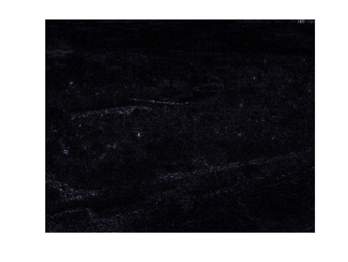
Figure 1: First and $473$rd singular vector of the image sequence

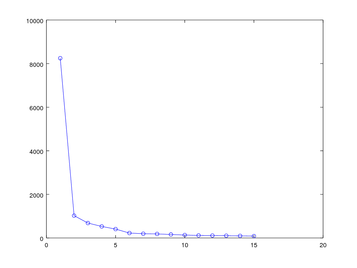
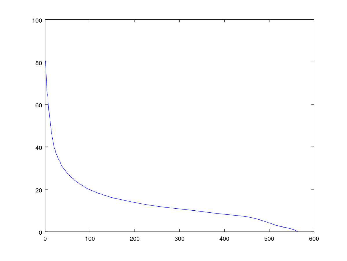
Figure 2: The first $15$ singular values (left) of the image and the remaining ones (right). Note the scaling of the $y$–axis.

Indeed, the singular values decay rapidly. This can be seen in Fig. 2, where we have decomposed the singular values into the dominant 15 and the remaining ones. The L-shape of this curve suggests to cut down to about $20$ singular values and to decompose the sequence by projecting on the first $20$ and on the remaining singular vectors. This essentially removes moving objects from the frames but still maintains more persistent features like shadows and illumination of the scenery which change over time, but in a slower and more persistent way. We show two example frames in Fig. 3 and Fig. 4, where the top left image is the original frame that is decomposed into a “still” image and an image with the “moving” parts. Note that the advantage of our algorithm is that, in contrast to methods like [6] which is based on [13], it allows to compute the projection of the frames to an arbitrary number of singular vectors, once the video is learned properly. Note that the number of relevant singular values can usually only be detected once the SVD is computed.

The original frames and video with the decomposition can also be downloaded for verification from the address given above.

Figure 3: Frame #351, decomposition: Detection of large (boat) and small (bus) moving features at the same time.

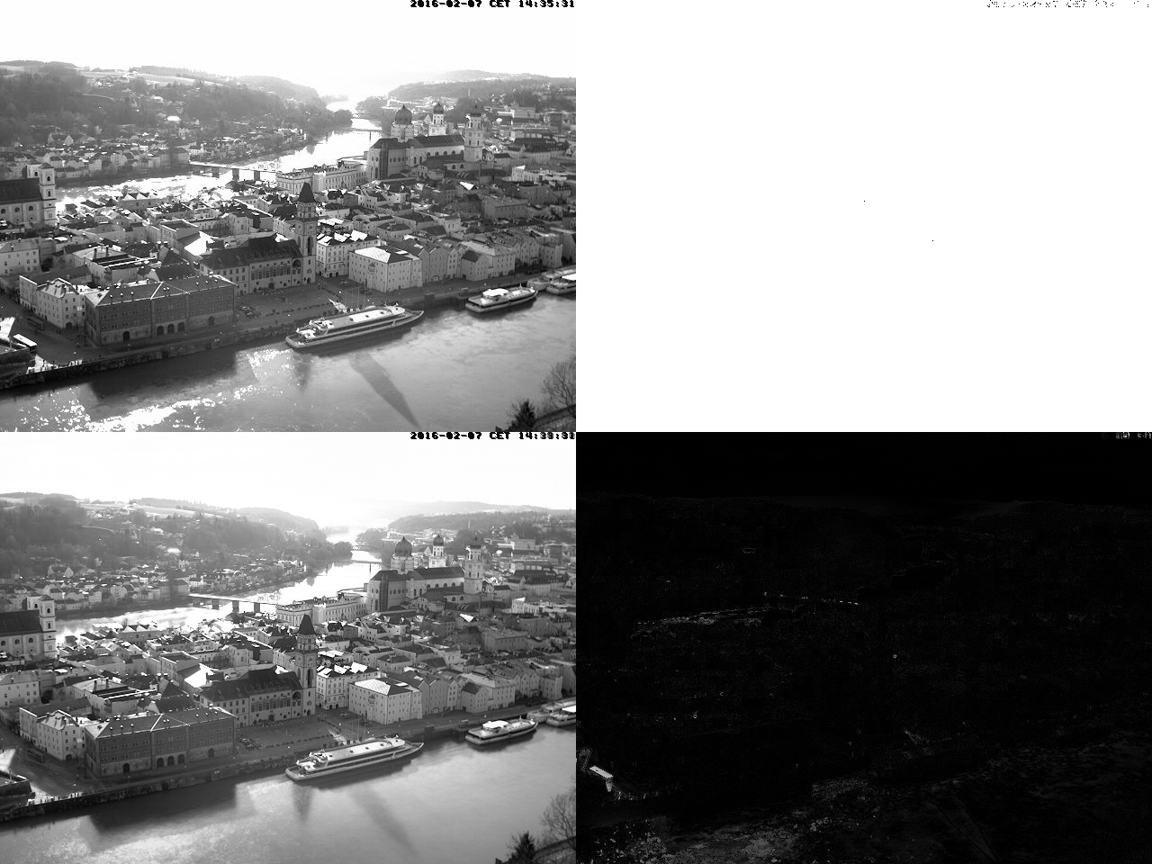
Figure 4: Frame #507, decomposition: Moving objects (bus) and light effects on the water caused by the afternoon sun. Note that the shadows are still reproduced in the “still” image.

4.3 Prony’s problem in several variables

The main motivation for Algorithm 1, however, was the multivariate version of Prony’s method [17] which has attracted some interest recently; besides being interesting by itself, it is the main mathematical problem behind the superresolution concept from [18], which in turn is motivated by studying point spread functions from microscopy. In a nutshell, Prony’s problem can be described as follows: given a function in $s$ variables of the form

$$f(x)=\sum_{\omega\in\Omega}f_{\omega}\,e^{\omega^{T}x},\qquad f_{\omega}\in\mathbb{C},\quad\Omega\subset\left(\mathbb{R}+i(\mathbb{R}/2\pi\mathbb{Z})\right)^{s},\,\#\Omega<\infty,$$ (66)

recover the unknown frequencies $\omega$ from the finite set $\Omega$ as well as the coefficients $f_{\omega}$, $\omega\in\Omega$, from integer samples of $f$, i.e., from $f(A)$, $A\subset\mathbb{Z}^{s}$. Note that the restriction on the imaginary part of the frequencies is required to make the solution unique and the problem well–defined. The main assumption made when solving this problem is sparsity, which means that $\#\Omega$ is small while no other assumptions on $\Omega$ are necessary, though of course the conditioning of the problem will depend on the geometry of $\Omega$.

Though determining $\Omega$ is a nonlinear problem, it can be approached by methods from Numerical Linear Algebra. As pointed out in [7, 8], the Hankel matrices

$$F_{A,B}:=\left[f(\alpha-\beta):\begin{array}[]{c}\alpha\in A\\ \beta\in B\end{array}\right],\qquad A,B\subset\mathbb{N}_{0}^{s},$$ (67)

provide all information about the ideal

$$I_{\Omega}:=\left\{p\in\mathbb{C}[x_{1},\dots,x_{s}]:p(e^{\omega})=0,\,\omega\in\Omega\right\},$$ (68)

provided that $A$ and $B$ are sufficiently rich. Once a basis for $I_{\Omega}$ is determined, the common zeros and therefore the frequencies can be determined by methods from Computer Algebra. In particular, if $A$ is such that the monomials $x^{\alpha}$, $\alpha\in A$ admit interpolation at $e^{\Omega}:=\{e^{\omega}:\omega\in\Omega\}\subset\mathbb{C}^{s}$, then a polynomial belongs to $I_{\Omega}$ if and only if its coefficient vector is in the kernel of $F_{A,B}$. By increasing $B$ in a proper way, one can so construct Gröbner or H–bases for $I_{\Omega}$ with which the computation of the frequencies is reduced to an eigenvalue problem. The main observation from [7, 8] is now as follows.

Theorem 4.1

If $A\subset\mathbb{N}_{0}^{s}$ is sufficiently rich in the sense that

$$\Pi=I_{\Omega}+\mbox{{span}\,}\{(\cdot)^{\alpha}:\alpha\in A\},$$

then, with $F_{A,B}$ as in (67),

1. $[p_{\alpha}:\alpha\in B]\in\ker F_{A,B}$ if and only if $p(x)=\sum p_{\alpha}x^{\alpha}\in I_{\Omega}$.

2. if ${\mathop{\rm rank\,}\nolimits}F_{A,\Gamma_{n}}={\mathop{\rm rank\,}\nolimits}F_{A,\Gamma_{n+1}}$, then $\ker F_{A,\Gamma_{n}}(x)$ is a basis of $I_{\Omega}$, where $\Gamma_{n}:=\{\alpha\in\mathbb{N}_{0}^{s}:|\alpha|\leq n\}$.

These two observations suggest the algorithm to solve Prony’s problem: first find a “good” set $A$ and then build successively the matrices

$$F_{A,\Gamma_{0}},F_{A,\Gamma_{1}},\dots,F_{A,\Gamma_{n}},F_{A,\Gamma_{n+1}},\dots$$

until ${\mathop{\rm rank\,}\nolimits}F_{A,\Gamma_{n}}={\mathop{\rm rank\,}\nolimits}F_{A,\Gamma_{n+1}}$. If

$$F_{A,\Gamma_{k}}=U\Sigma V^{T},$$

then the components of $V$ belonging to zero singular values are, by Theorem 4.1, coefficient vectors of polynomials from the ideal, and once the rank stabilizes, a basis of the ideal has been found from which the set $\Omega$ can be computed. Hence, in contrast to the PCA application before, where the singular vectors in $U$ were of importance, we are now interested in the matrix $V$ and it’s capability to distinguish between the kernel of $F_{A,\Gamma_{k}}$ and its orthogonal complement.

There is one major drawback, however: in several variables, the geometry of $e^{\Omega}$ becomes increasingly relevant and usually, only $\#\Omega$ or an upper bound for it are assumed to be known. The smallest known choice for $A$ that works unconditionally without any further assumptions on $\Omega$ has cardinality $\#\Omega\,\left(\log\#\Omega\right)^{s-1}$ which still grows quite fast for large $s$. Moreover, it is known to be beneficial to oversample, i.e., to choose $A$ larger than needed, cf. [19]. Thus, Algorithm 1 addresses the two main issues here: how to handle large columns in a still efficient way and how to ensure that the rank is controlled well.

References

References

-
[1]
J. W. Eaton, D. Bateman, S. Hauberg,
GNU Octave
version 3.0.1 manual: a high-level interactive language for numerical
computations, CreateSpace Independent Publishing Platform, 2009, ISBN
1441413006.
URL http://www.gnu.org/software/octave/doc/interpreter - [2] G. Golub, C. F. van Loan, Matrix Computations, 3rd Edition, The Johns Hopkins University Press, 1996.
- [3] P. Businger, Algol programming, contribution no. 26. Updating a singular value decomposition, BIT 10 (1970) 376–385.
- [4] A. Björck, Numerical Methods for Least Squares Problems, SIAM, 1996.
- [5] M. Brand, Fast low-rank modifications of the thin singular value decomposition, Linear Algebra Appl. 415 (2006) 20–30.
- [6] P. Rodriguez, B. Wohlberg, Incremental principal component pursuit for video background modeling, J. Math. Imaging Vis. 55 (2016) 1–18.
- [7] T. Sauer, Prony’s method in several variables, Numer. Math. 136 (2017) 411–438, arXiv:1602.02352. doi:10.1007/s00211-016-0844-8.
- [8] T. Sauer, Prony’s method in several variables: symbolic solutions by universal interpolation, J. Symbolic Comput. 84 (2018) 95–112, arXiv:1603.03944. doi:10.1016/j.jsc.2017.03.006.
- [9] G. W. Stewart, Updating a rank–revealing decomposition, SIAM J. Matrix Anal. Appl. 14 (1993) 494–499.
- [10] R. Schmidt, Multiple emitter location and signal parameter estimation, IEEE Transactions on Antennas and Propagation 34 (1986) 276–280.
- [11] J. R. Bunch, C. P. Nielsen, Updating the singular value decomposition, Numer. Math. 31 (1978) 111–129.
- [12] J. W. Daniel, W. B. Gragg, L. Kaufman, G. W. Stewart, Reorthogonalization and stable algorithms for updating the Gram-Schmidt QR factorization, Math. Comp. 30 (1976) 772–795.
- [13] C. G. Baker, K. A. Gallivan, P. Van Dooren, Low-rank incremental methods for computing dominant singular subspaces, Linear Algebra Appl. 436 (2012) 2866–2888.
- [14] S. Chandrasekaran, I. C. F. Ipsen, On rank-revealing factorizations, SIAM J. Matrix Anal. Appl. 15 (1994) 592–622.
- [15] N. J. Higham, Accuracy and stability of numerical algorithms, 2nd Edition, SIAM, 2002.
- [16] T. Hastie, R. Tibshirani, J. Friedman, The Elements of Statistical Learning, 2nd Edition, Springer, 2009.
- [17] C. Prony, Essai expérimental et analytique sur les lois de la dilabilité des fluides élastiques, et sur celles de la force expansive de la vapeur de l’eau et de la vapeur de l’alkool, à différentes températures, J. de l’École polytechnique 2 (1795) 24–77.
- [18] E. J. Candès, C. Fernandez-Granda, Towards a mathematical theory of super-resolution, Comm. Pure Appl. Math. 67 (2012) 906–956.
- [19] D. Batenkov, Stability and super-resolution of generalized spike recovery, Appl. Comput. Harmon. Anal.In press, arXiv:1409.3137v2. doi:10.1016/j.acha.2016.09.004.