Acoustic Propagation in lined ducts with varying cross-section using a Mild-Slope approximation.

Abstract

A modelling of low-frequency sound propagation in slowly varying ducts with smoothly varying lining is proposed leading to an acoustic mild-slope equation analogue to the with mild-slope equation for water waves. This simple 1D Mild Slope Equation is derived by direct application of the Galerkin method. It is shown that the acoustic mild-slope equation can serve as a good alternative to computationally expensive Helmholtz equations to solve such kind of problem. The results from this equation agrees well with FEM based solutions of Helmholtz equation.

I Introduction

The theory of sound propagation in straight ducts with constant impedance type boundary conditions and a homogeneous (stationary) medium is classical and well-established Morse and Ingard (1968). In certain applications the assumption of a straight duct and constant impedance is not valid, and it is therefore of practical interest to consider sound transmission through lined ducts of varying cross-section. A well-known approximation to acoustic propagation in smoothly varying hard wall duct is given by the horn equation Morse and Ingard (1968); Webster (1919), which still is a subject of interest for several applications Rienstra (2005); Gupta et al. (2015). When the smooth variation in duct cross-section is coupled with variable impedance, computationally expensive numerical methods remains the preferred choice. Indeed, although acoustic propagation in slowly varying ducts has been widely investigated for many decades Rienstra (2003); Ovenden and Rienstra (2004); Rienstra (2001); Peake and Cooper (2001); Brambley and Peake (2008); Nayfeh and Telionis (1973); Rienstra and Eversman (2001), efficient approximate equation to solve this problem does not exist yet.

In the context of water waves, to investigate the effect of mild slope water-beds on propagation, a classical tool is the Mild-Slope Equation (MSE) Jung and Suh (2008); Chamberlain (1993); Berkhoff (1976); Booij (1983) . An improved version of this formulation called Modified Mild-Slope Equation (MMSE) Chamberlain and Porter (1995); Liu and Xie (2013); Suh et al. (2005); Liu et al. (2012) was later used to study variety of depth variations such as smooth beds Liu and Xie (2013) and even circular bowl pits Suh et al. (2005). In the following we will use the similarity between water waves on varying bathymetry and acoustic propagation in smoothly varying lined ducts. By this simple analogy an Acoustic Mild Slope Equation (AMSE) is derived by direct application of the classical Galerkin method based on vertical integration used by Berkhoff Berkhoff (1976). An improved form of this equation, termed Modified Acoustic Mild Slope Equation (MAMSE) is also derived. The approximate results obtained from the AMSE and the MAMSE are compared with numerical solutions of Helmholtz Equation and the results are in close agreement. This 1D approximation equation promises easier implementation and computationally efficient way to solve problems of lined ducts with or without slowly varying cross-sections.

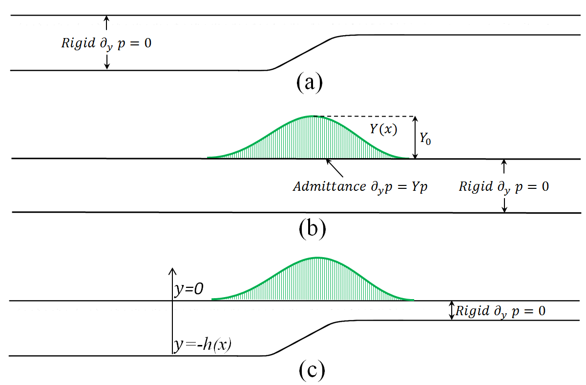
Figure 1: Schematic under investigation, (a) Smoothly varying rigid duct, (b) A lined duct and (c) Lined duct with smoothly varying cross-section.

II Theory

We consider the sound propagation in a 2D channel, see (Fig. 1(b)). The lower wall is rigid while the upper wall is compliant and described by a varying admittance $Y(x)$. When the distances are non-dimensioned by the height of the channel $H$, the Helmholtz equation, governing the propagation of the acoustic pressure $p$, is:

$$\Delta p+{k^{2}}p=0$$ (1)

where $k=\omega H/c_{0}$ is the reduced frequency, $\omega$ is the frequency and $c_{0}$ is the sound velocity. The boundary conditions are $\partial_{n}p=0$ for $y=-h(x)$ and $\partial_{y}p=Yp$ for $y=0$.

For a uniform admittance Y, a solution of the form $p=A\cosh(\alpha(y))\exp(\mathrm{i}(-\omega t+\beta x))$ is searched where $\alpha^{2}=\beta^{2}-k^{2}$ and this leads to the dispersion relation:

$$Y={\alpha}\>\text{tanh}({\alpha{h}})$$ (2)

In the following this equation will be also used for varying $Y$ and $h$ to get a local value $\alpha(x)$. With some manipulations it is possible to obtain a simple 1D equation that explains the three cases depicted in Fig. 1. Indeed, following the same lines as in Chamberlain and Porter (1995), we obtain a 1D acoustic mild slope equation (AMSE) that is written as

$${\nabla_{x}}.{\left({{u_{0}(x)}{\nabla_{x}}{p_{o}}}\right)}+\left(({{\alpha^{2}+k^{2})}{u_{0}(x)}}\right){p_{o}}=0$$ (3)

Where

$$\begin{gathered}{u_{0}}(x)=\int\limits_{-h(x)}^{0}{{w_{0}}^{2}}dy=\frac{1}{{2\alpha^{2}}}\left[{h(x)(\alpha^{2}-Y^{2})+Y}\right]\\ =\frac{1}{{2\alpha}}\left[\frac{(Yh(x))^{\prime}}{(\alpha{h(x)})^{\prime}}\right]\end{gathered}$$ (4)

$$p=p_{0}(x)w_{0}(y;x)$$

and

$$w_{0}(y;x)=\text{sech}{(\alpha{h(x)})}\cosh(\alpha(x)(y+h(x))).$$

Here, the wavenumber $\alpha$ is the real, positive root of the local dispersion relation.

Since its derivation, the MSE has proved to be a very powerful tool to model linear water wave propagation, because in addition to providing information about both refraction and diffraction effects also it was significantly accurate for short water waves as well as long water waves. For acoustics, the AMSE that we propose will be limited to low frequencies where only one mode is propagating in the waveguide. Besides, without lining (for hard wall ducts $Y=0$), the AMSE should be able to recover the classical horn equation Rienstra (2005). Indeed, it is the case: taking the limit of small $Y$ going to zero, the dispersion relation (Eqn. 2) becomes, $Y=\alpha^{2}h(x)$, for $\alpha\ll{\text{1}}$, which implies, $u_{0}(x)=h(x)$. Putting this value in Eqn. (3) we obtain

$$p(x)^{\prime\prime}+\frac{h(x)^{\prime}}{h(x)}p(x)^{\prime}+k^{2}{p(x)}=0$$ (5)

that shows that the AMSE transforms to the classical acoustic horn equation for the hard wall case ($Y\rightarrow 0$).

There had been an extension to MSE which is called the modified mild-slope equation (MMSE) initially derived by Chamberlain and Porter Chamberlain and Porter (1995), in which both the obstacle curvature term related to $\Delta^{2}h$ and the slope-squared term related to $(\Delta{h})^{2}$ are added into the traditional AMSE (Eqn. 3). In the water wave problems, it is shown that this equation is capable of describing known scattering properties of singly and doubly periodic ripple beds, for which the mild-slope equation fails. Retaining a $r(x)$ term we get the Modified Acoustic Mild Slope Equation (MAMSE).

$${\nabla_{x}}.{\left({{u_{0}}{\nabla_{x}}{p_{o}}}\right)}+\left(({{\alpha^{2}+k^{2})}{u_{0}}+r(x)}\right){p_{o}}=0$$ (6)

where

$$\begin{gathered}r(x)=\int_{-h(x)}^{0}{{w_{0}}{\nabla_{x}}^{2}{w_{0}}dy}\,\,\end{gathered}$$ (7)

III Results and Discussions

In this section, the results from the AMSE and the MAMSE are discussed and are compared with solutions of the Helmholtz Equation using Finite Element Method (FEM) based COMSOL.

Among others, a practical realization of the admittance can be done by using small closed tubes of variable lengths $b(x)$ perpendicular to the upper wall. Considering lossless tubes, the admittance can be written as:

$$Y(x,{k})=k\>\tan(k\>b).$$ (8)

In what follows, a variation of the tube length $b(x)$ is selected as

$$b(x)=\frac{b_{0}}{2}(1+cos(\frac{\pi{x}}{{{\text{L}}_{{\text{imp}}}}}))$$ (9)

where ${{\text{L}}_{{\text{imp}}}}$ and $b_{0}$ are the lengths which characterizes the distance and max height over which the admittance varies. Besides, the shape of the obstacle will be given by

$$h(x)=\frac{H_{obs}}{2}(1+cos(\frac{\pi{x}}{{{\text{L}}_{{\text{obs}}}}}))$$ (10)

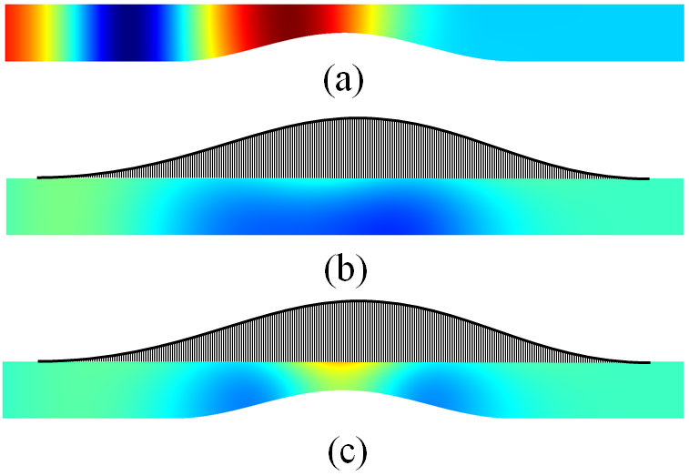
Figure 2: Real Pressure field ($k=0.2\pi$) for three configurations, (a) Smoothly varying rigid duct, (b) A lined duct and (c) Lined duct with smoothly varying cross-section.

III.1 Mild Slope - AMSE

A number of numerical experiments were carried out in order to check the 1D mild-slope equation against the 2D Helmholtz equation. A reference solution will be given by the numerical FEM computation form the Helmholtz equation, where triangular mesh is chosen as finite elements in the computational domain. The Mild-slope equation (Eqn. 3) is discretised using fourth order Runge-Kutta method. In order to minimize the computational time, an explicit wave number formulae is used Farooqui et al. . The numerical accuracy of both models was determined by varying the mesh size. Due to one-dimensionality the mild-slope approximation required lower number of dimensions, a smaller mesh size and it is therefore computationally much cheaper. In the test cases presented, the obstacle heights are chosen such that the horn equation validity Rienstra (2005) of ($kh\ll{1}$, $h^{\prime}\ll{1}$) is verified for the hard cases .

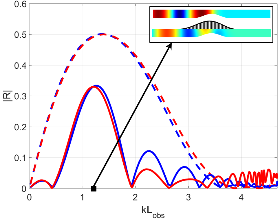
Figure 3: Absolute reflection $|\text{R}|$ from AMSE solutions for Hard duct red (dashed), lined duct red (solid), FEM solutions for Hard duct blue (dashed) and for lined duct blue (solid) for the parameters ${{\text{L}}_{{\text{obs}}}}=3,{{\text{L}}_{{\text{imp}}}}=5,H_{obs}=0.5,H_{obs}^{\prime}=0.26178,Y=0.4645,Y^{\prime}=0.1432$ (Inset at ${\text{k}}{{\text{L}}_{{\text{obs}}}}=1.28$)

Using FEM, 2D Helmholtz Equation was solved to calculate pressure distributions for the three cases shown in Fig. 2. Fig. 2(a), (b) and (c), shows the smoothly-varying hard duct, smoothly-varying impedance and the combination of the two cases, respectively. Although, Fig. 2(c) is the perfect demonstration of application of the AMSE (Eqn. 3), it can also efficiently describe the scattering phenomenon of all these configuations. The comparison of results from AMSE and FEM is shown in Fig. 3. The results shows the variation of absolute reflection coefficient $|\text{R}|$ with the ${\text{k}}{{\text{L}}_{{\text{obs}}}}$, where ${{\text{L}}_{{\text{obs}}}}$ is the length of the obstacle in the duct, which is also referred as length of variation of the duct cross section. AMSE calculations for hard duct (red (dashed)) with $\alpha=0$ (Webster horn equation), is in close agreement with the FEM computations (blue (dashed)), under the accuracy limits of the horn equation ($kh\ll{1}$, $h^{\prime}\ll{1}$) Rienstra (2005). As our range of interest lies under the horn equation regime, the values of $Y$ and $Y^{\prime}$ mentioned in figure captions are their maximum values corresponding $k_{max}=1$. The red (dashed) from AMSE and blue (dashed) from FEM refers to hard duct with an obstacle. They seem to agree well till the Webster limit. This curve corresponds to smoothly varying rigid duct case as depicted in Fig. 2(a). The red (solid) from AMSE solutions and blue (solid) from FEM solutions refers to lined duct with obstacle (Fig. 2(c)). It can be seen that there is significant mismatch between the two from ${\text{k}}{{\text{L}}_{{\text{obs}}}}\geqslant{\text{2}}$. This mismatch would need further insights to be quantified in order to better understand the limits of the AMSE with respect to Helmholtz equation.

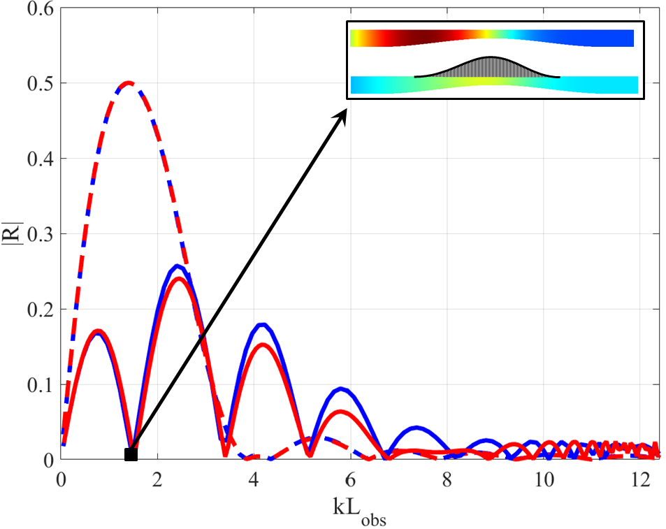
Figure 4: Absolute reflection $|\text{R}|$ from AMSE solutions for Hard duct red (dashed), lined duct red (solid), FEM solutions for Hard duct, blue (dashed) and for lined duct, blue (solid) for the parameters ${{\text{L}}_{{\text{obs}}}}=8,{{\text{L}}_{{\text{imp}}}}=5,H_{obs}=0.5,H_{obs}^{\prime}=0.098175,Y=0.4645,Y^{\prime}=0.1432$ , (Inset at ${\text{k}}{{\text{L}}_{{\text{obs}}}}=1.48$)

Fig. 4 and Fig. 5 shows the variation of absolute reflection coefficient $|\text{R}|$ with ${\text{k}}{{\text{L}}_{{\text{obs}}}}$, for ${{\text{L}}_{{\text{obs}}}}=$ 8 and 10, respectively. On comparison with Fig. 3(b), it can be concluded, that for ${{\text{L}}_{{\text{obs}}}}=$ 8, highly accurate predictions are possible with AMSE, when ${\text{k}}{{\text{L}}_{{\text{obs}}}}\leqslant$ 5. The scaling of Fig. 5 can be obtained re-calculating the result of Fig. 3(b) with $h=0.98$, which yields ${\text{k}}{{\text{L}}_{{\text{obs}}}}\leqslant$ 10. In some cases the solutions from AMSE agrees quite well even beyond the Webster limit. The reason to this behavior is extremely low values of $(Y(x)h(x))^{\prime}$, which aids in extending the proposed limits of AMSE.

Figure 5: Absolute reflection $|\text{R}|$ from AMSE solutions for Hard duct red (dashed), lined duct red (solid), FEM solutions for Hard duct blue (dashed) and for lined duct blue (solid) for the parameters ${{\text{L}}_{{\text{obs}}}}=10,{{\text{L}}_{{\text{imp}}}}=5,H_{obs}=0.98,{\delta}H_{obs}=0.15393,B_{imp}^{\prime}=0.31416$, (Inset at ${\text{k}}{{\text{L}}_{{\text{obs}}}}=1.45$)

III.2 Modified Mild Slope - MAMSE

In the domain of water waves, the scattering of water waves by ripples in a horizontal bed falls outside the scope of the mild-slope equation. $Kirby(1986)$ derived an alternative equation which allowed for a rapidly varying, small-amplitude bedform to be superimposed on a slowly varying component of topography. As explained earlier, the full form of AMSE including the $r(x)$ term is called modified acoustic mild slope equation MAMSE (Eqn. 6).

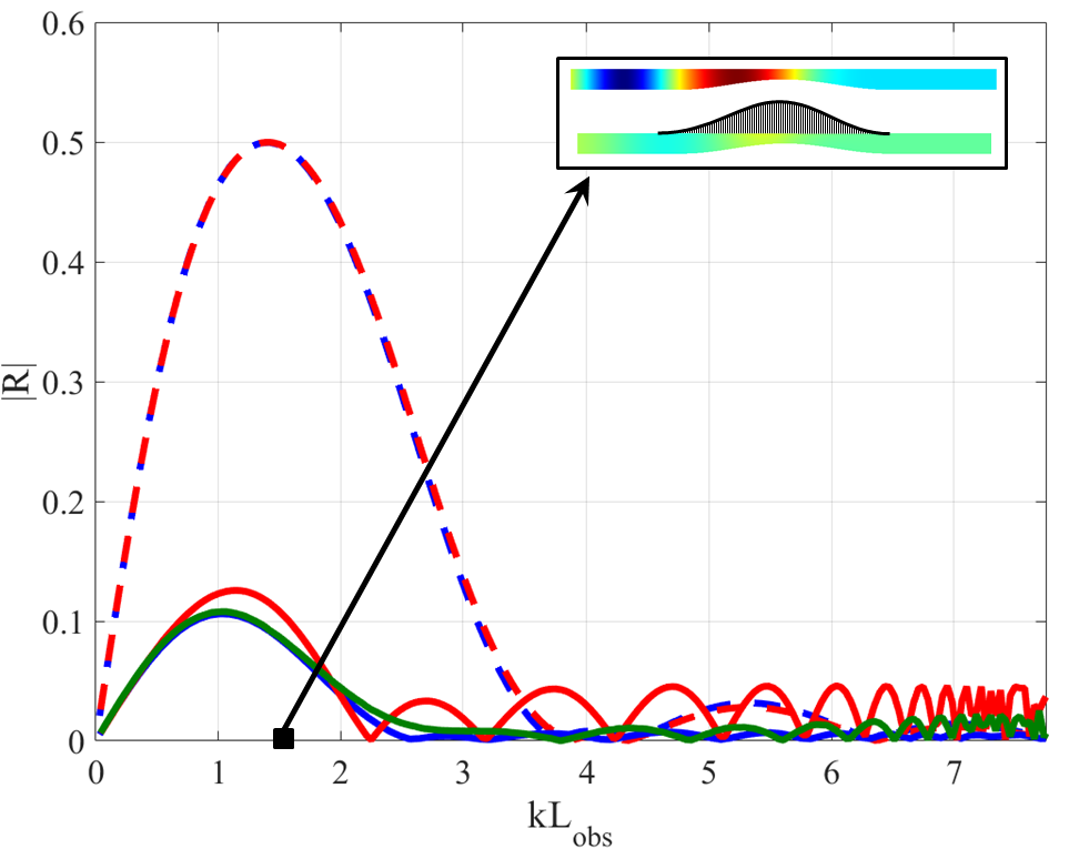
Figure 6: Absolute reflection $|\text{R}|$ from AMSE solutions for Hard duct red (dashed), lined duct red (solid), FEM solutions for Hard duct blue (dashed) and for lined duct blue (solid) and MAMSE solutions for lined duct green (solid) for the parameters , ${{\text{L}}_{{\text{obs}}}}=5,{{\text{L}}_{{\text{imp}}}}=5,H_{obs}=0.5,H_{obs}^{\prime}=0.15708,Y=0.4645,Y^{\prime}=0.1432$, (Inset at ${\text{k}}{{\text{L}}_{{\text{obs}}}}=1.57$)

Fig. 6 shows the variation of absolute reflection coefficient $|\text{R}|$ with ${\text{k}}{{\text{L}}_{{\text{obs}}}}$, for ${{\text{L}}_{{\text{obs}}}}=$ 5. As evident from the figure, the Mild slope equation (red solid) has a limited accuracy range (${\text{k}}{{\text{L}}_{{\text{obs}}}}\leqslant$ 2). Here, the MAMSE (green solid) surpasses the mild-slope limits and is a much better approximation of the FEM solution (blue curve). Although, application of MAMSE is more difficult and computationally expensive, but as in the case discussed, might serve to extend the AMSE limits for broad frequency range.

In addition to extension of AMSE limits, the inclusion of obstacle curvature term related to $\Delta^{2}h$ and the slope-squared term related to $(\Delta{h})^{2}$ helps in improving the accuracy of the solution. For instance, Fig. 7 shows the variation of absolute reflection coefficient $|\text{R}|$ with k, for ${{\text{L}}_{{\text{obs}}}}=$ 5. The results are for a straight duct with just a smoothly varying liner. Here, the MAMSE (green solid) is a much better approximation in terms on the broadband prediction as well as accuracy in comparison to Helmholtz equation.

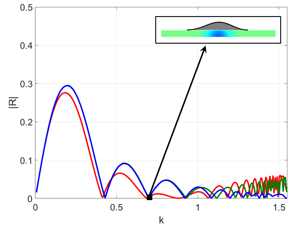
Figure 7: Absolute reflection $|\text{R}|$ from FEM solutions for straight lined duct blue (solid), AMSE solutions for Non-varying lined duct red (solid), and MAMSE solutions for Non-varying lined duct green (solid) for the parameters , ${{\text{L}}_{{\text{imp}}}}=5,Y=0.4645,Y^{\prime}=0.1432$

IV Conclusion

The mild slope equation is a popular tool to model water wave propagation on a mild-slope bed. In analogy with water waves, a one-dimensional mild-slope formulation is proposed in this work to model low-frequency sound propagation in slowly varying ducts with smoothly varying lining. This approximation is derived by direct application of the classical Galerkins method. It is shown that the 1D mild-slope equation is an economical and efficient alternative to computationally expensive and complex 2D Helmholtz equations to solve such kind of problem.

References

- Morse and Ingard (1968) P. M. Morse and K. U. Ingard, Theoretical acoustics (Princeton university press, 1968) chap: Sound waves in Ducts and Rooms, 467–599.
- Webster (1919) A. G. Webster, Proceedings of the National Academy of Sciences 5, 275 (1919).
- Rienstra (2005) S. W. Rienstra, SIAM Journal on Applied Mathematics 65, 1981 (2005).
- Gupta et al. (2015) A. Gupta, K.-M. Lim, and C. H. Chew, Wave Motion 55, 1 (2015).
- Rienstra (2003) S. W. Rienstra, Journal of Fluid Mechanics 495, 157 (2003).
- Ovenden and Rienstra (2004) N. C. Ovenden and S. W. Rienstra, AIAA journal 42, 1832 (2004).
- Rienstra (2001) S. W. Rienstra, Cut-on, cut-off transition of sound in slowly varying flow ducts (Eindhoven University of Technology, Department of Mathematics and Computing Science, 2001).
- Peake and Cooper (2001) N. Peake and A. Cooper, Journal of Sound and Vibration 243, 381 (2001).
- Brambley and Peake (2008) E. Brambley and N. Peake, Journal of Fluid Mechanics 596, 387 (2008).
- Nayfeh and Telionis (1973) A. H. Nayfeh and D. P. Telionis, The Journal of the Acoustical Society of America 54, 1654 (1973).
- Rienstra and Eversman (2001) S. W. Rienstra and W. Eversman, Journal of Fluid Mechanics 437, 367 (2001).
- Jung and Suh (2008) T.-H. Jung and K.-D. Suh, Wave Motion 45, 835 (2008).
- Chamberlain (1993) P. Chamberlain, Wave Motion 17, 267 (1993).
- Berkhoff (1976) J. C. W. Berkhoff, (1976).
- Booij (1983) N. Booij, Coastal Engineering 7, 191 (1983).
- Chamberlain and Porter (1995) P. Chamberlain and D. Porter, Journal of Fluid Mechanics 291, 393 (1995).
- Liu and Xie (2013) H.-W. Liu and J.-J. Xie, Wave Motion 50, 869 (2013).
- Suh et al. (2005) K.-D. Suh, T.-H. Jung, and M. C. Haller, Wave Motion 42, 143 (2005).
- Liu et al. (2012) H.-W. Liu, J. Yang, and P. Lin, Wave Motion 49, 445 (2012).
- (20) M. Farooqui, Y. Aurégan, and V. Pagneux, Submitted to- Journal of Acoustical Society of America- Express Letters .