Density decay and growth of correlations
in the Game of Life
xxx

Abstract

We study the Game of Life as a statistical system on an $L\times L$ square lattice with periodic boundary conditions. Starting from a random initial configuration of density $\rho_{\rm in}=0.3$ we investigate the relaxation of the density as well as the growth with time of spatial correlations. The asymptotic density relaxation is exponential with a characteristic time $\tau_{L}$ whose system size dependence follows a power law $\tau_{L}\propto L^{z}$ with $z=1.66\pm 0.05$ before saturating at large system sizes to a constant $\tau_{\infty}$. The correlation growth is characterized by a time dependent correlation length $\xi_{t}$ that follows a power law $\xi_{t}\propto t^{1/z^{\prime}}$ with $z^{\prime}$ close to $z$ before saturating at large times to a constant $\xi_{\infty}$. We discuss the difficulty of determining the correlation length $\xi_{\infty}$ in the final “quiescent” state of the system. The decay time $t_{\rm q}$ towards the quiescent state is a random variable; we present simulational evidence as well as a heuristic argument indicating that for large $L$ its distribution peaks at a value $t_{\rm q}^{*}(L)\simeq 2\tau_{\infty}\log L$.

Keywords: cellular automata; Game of Life; critical phenomena.

1 Introduction

T he Game of Life (GL) is a cellular automaton proposed in 1970 by Conway [1] and made popular by Gardner [2]. It evolves deterministically in discrete time $t=0,1,2,...$ according to the following rules. On a two-dimensional square lattice, at any instant of time $t$, each site ${\bf{r}}$ may be occupied or empty (occupation number $n_{t}({\bf{r}})=1$ or $n_{t}({\bf{r}})=0$). The sites are often referred to as “cells” and the occupied and empty states are said to correspond to the cell being “alive” and “dead,” respectively. The state of a site ${\bf{r}}$ at time $t+1$ follows deterministically from its own state and the states of its eight neighbors (the Moore neighborhood) at time $t$; the update rule is formulated with the aid of the auxiliary quantity $S_{t}({\bf{r}})\in\{0,1,...,8\}$, defined as the sum at time $t$ of the occupation numbers of the neighbors of ${\bf{r}}$. In terms of this sum Conway’s update rule reads

– if $S_{t}({\bf{r}})\neq 2,3$, then $n_{t+1}({\bf{r}})=0$ ;

– if $S_{t}({\bf{r}})=2$, then $n_{t+1}({\bf{r}})=n_{t}({\bf{r}})$ ;

– if $S_{t}({\bf{r}})=3$, then $n_{t+1}({\bf{r}})=1$,
and is carried out synchronously for all sites.

The qualification “totalistic” is used to indicate that the occupation numbers of the neighboring sites enter the update rule only through their sum. The number of possible totalistic cellular automata based on the Moore neighborhood is equal to $2^{18}$. Several authors [3, 4, 5] have contributed to classifying the automata in this category. Conway noticed that there is (i) a large “supercritical” subclass for which, typically, an initially localized set of living cells will progressively fill the whole available lattice with living cells at some average density; and (ii) the complementary subclass for which no such explosive growth happens.

The GL update rule stated above stemmed from Conway’s attempt to find the most interesting update rule. In physical parlance, this meant that he was trying to be as close as possible to the critical line separating the two subclasses, while refusing to be supercritical.

Interest in the statistical properties of the GL goes back at least to the work of Dresden and Wong [6], who adopted an analytical approach, and that of Schulman and Seiden [7], who incorporated stochasticity in the rules of the game and were followed therein by many later researchers. Much interest in the GL was subsequently generated by Bak et al. [8]. On the basis of their simulation of the effect of small external perturbations repetitively applied to the GL these authors claimed that due to “self-organization” [9, 10] the GL is exactly at  a critical point. This idea has been advanced many times [11, 12, 13, 14, 15, 16], either as a fact or as a hypothesis, but was abandoned following the investigations of, in particular, Bennett and Bourzutschky [17], Hemmingsson [18], Nordfalk and Alstrøm [19], and Blok and Bergersen [20]. Our work confirms, if that was still needed, that the GL is subcritical; however, and as many authors have noted, it is close to criticality. In this study we investigate its near-critical properties while staying strictly within the limits of the original GL: we are interested in deterministic dynamics and do not study any stochastic extensions of the GL, nor subject it to external perturbations.

We will in this work study the GL on a periodic $L\times L$ lattice. letting it start from an arbitrary random initial configuration. It is well-known that under such circumstances the GL, after a transient which may take thousands of time steps, enters a limit cycle, also referred to as a “quiescent” or a “stationary” state. The quiescent state is composed of small independent (i.e. nonoverlapping) groups of living cells that we will call “objects” and that may be static or periodically oscillating (see e.g. [8, 13, 21]). The vast majority of these objects belong to a dozen or so different types with linear sizes in the range from two to five lattice units. The oscillators among them have almost all a period of two time units; oscillators of higher periodicities do exist but are statistically insignificant. Related to the oscillators is the class of objects that are time-periodic modulo a translation in space. In GL jargon these are referred to as “spaceships,” their simplest and foremost example being the “glider.” On dedicated websites (see e.g. [22]) a great deal of attention is paid to these special objects. On a lattice with periodic boundary conditions they may certainly occur during the relaxation process, but their probability of survival into the quiescent state is far too small for them to have an impact on the properties studied in this work.

This paper is organized as follows.

In section 2 we consider the relaxation of the density of living cells to its quiescent state value. The relaxation curve is well-known  [21], but its asymptotic long time decay is subject to finite size effects that have never been reported. The observation of these effects requires strongly improved statistics, presented in section 2. We extract from our simulations the $L$ dependent decay time $\tau_{L}$ associated with the asymptotic density decay. For $L\lesssim 60$ this decay time appears to have the power law behavior $\tau_{L}\propto L^{z}$ with $z\approx 1.66$, whereas after a crossover regime it saturates for $L\gtrsim 180$ to a constant $\tau_{\infty}\approx 1800$.

In section 3 we consider how density pair correlations develop in the course of time. We are not aware of any earlier study of these time dependent correlations. We establish that there is a correlation length $\xi_{t}$ that grows with time as $\xi_{t}\propto t^{1/z^{\prime}}$ and saturates for $t\gtrsim 8000$ to a constant $\xi_{\infty}\approx 50$. Our value for $z^{\prime}$ is close to that of $z$ and we strongly suspect that they are in fact one and the same exponent, the difference being due to some unknown systematic bias in our analysis. At the end of section 3 we emphasize the difficulty of collecting statistics on the correlations in the quiescent state.

In section 4 we consider the probability distribution $P_{L}(t_{\rm q})$ of the decay times $t_{\rm q}$ to quiescent state. It appears that for large $t_{\rm q}$, with very good accuracy, this distribution decays exponentially with decay constant $1/\tau_{L}$. A heuristic argument leads us to conclude that for large $L$ the time $t_{\rm q}^{*}$ at which $P_{L}$ reaches its peak scales as $t_{\rm q}^{*}(L)\propto\log L$. The predicted curve for $t_{\rm q}^{*}(L)$ is in excellent agreement with the simulation data.

In section 5 we discuss our results and compare them to related work in the literature. We address several closely related points of interest and also briefly return to the question of self-organized criticality.

2 Density decay

$L$	$\rho_{L}(\infty)$	$N$000
128	0.028873 $\pm$ 0.000009	100 000
144	0.028828 $\pm$ 0.000027	10 000
160	0.028845 $\pm$ 0.000022	10 000
176	0.028758 $\pm$ 0.000025	10 000
192	0.028771 $\pm$ 0.000012	10 000
208	0.028734 $\pm$ 0.000017	10 000
224	0.028754 $\pm$ 0.000009	10 000
240	0.028711 $\pm$ 0.000018	12 500
256	0.028739 $\pm$ 0.000008	40 000
512	0.028721 $\pm$ 0.000006	40 000
$\infty$	0.028720 $\pm$ 0.000010

Table 1: List of quiescent state densities $\rho_{L}(\infty)$ with $N$ the number of quiescent states having contributed to the average. The last line is our extrapolation to infinite system size, $\lim_{L\to\infty}\rho_{L}(\infty)\equiv\rho^{*}=0.02872(1)$.

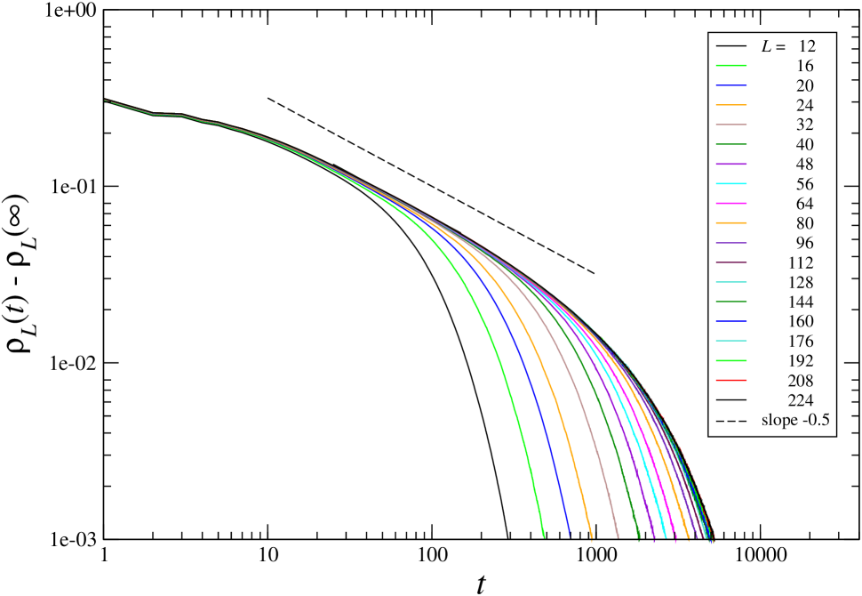
Figure 1: Density difference $\rho_{L}(t)-\rho_{L}(\infty)$ on a log-log scale for values of the system size $L$ that increase from left to right. For $L\gtrsim 100$ the curves become difficult to distinguish from their $L=\infty$ limit. The dashed line has slope $-0.5$.

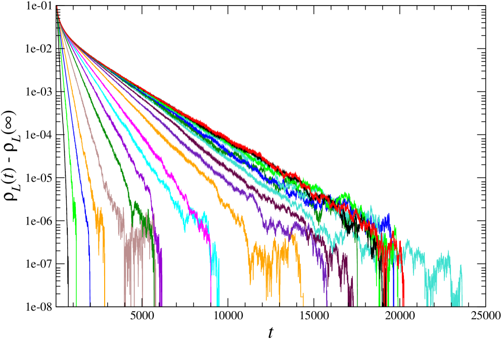
Figure 2: Density difference $\rho_{L}(t)-\rho_{L}(\infty)$ on a linear-log scale. Note that the vertical scale here goes down to much smaller values than in figure 1. The curves are for the same values of $L$ with the same color code as in figure 1. Curves for larger values of $L$ overlap among themselves and with the limit curve, and are not shown.

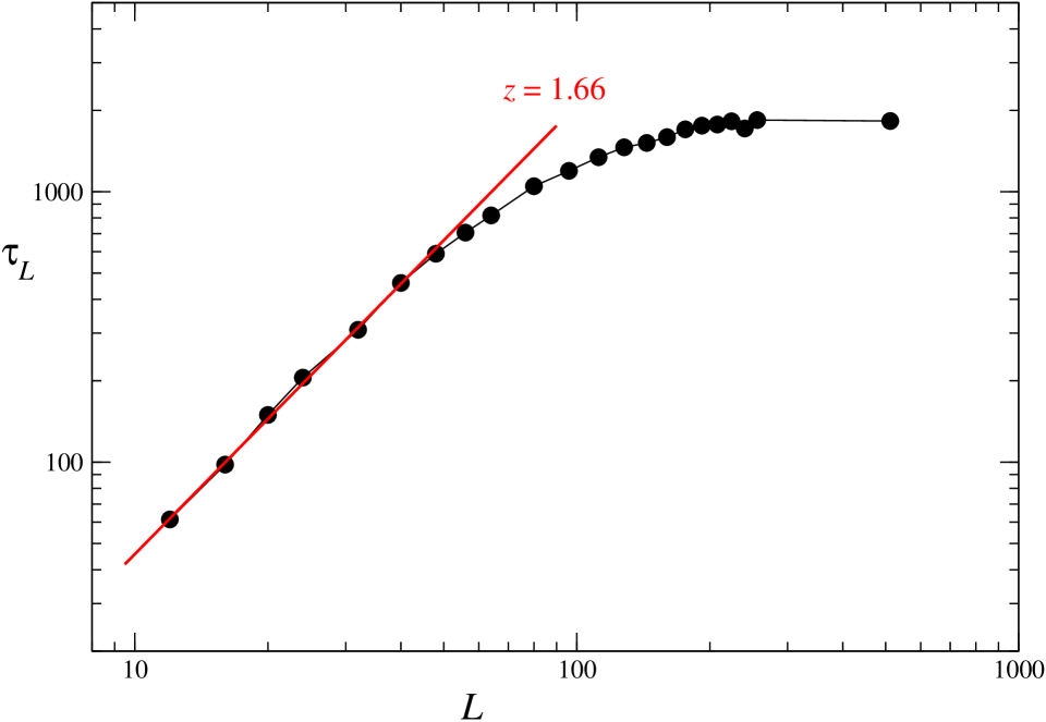
Figure 3: Data points: the relaxation times $\tau_{L}$ extracted from figure 2 shown on a log-log scale. Red line: best linear fit, having a slope $1.66$.

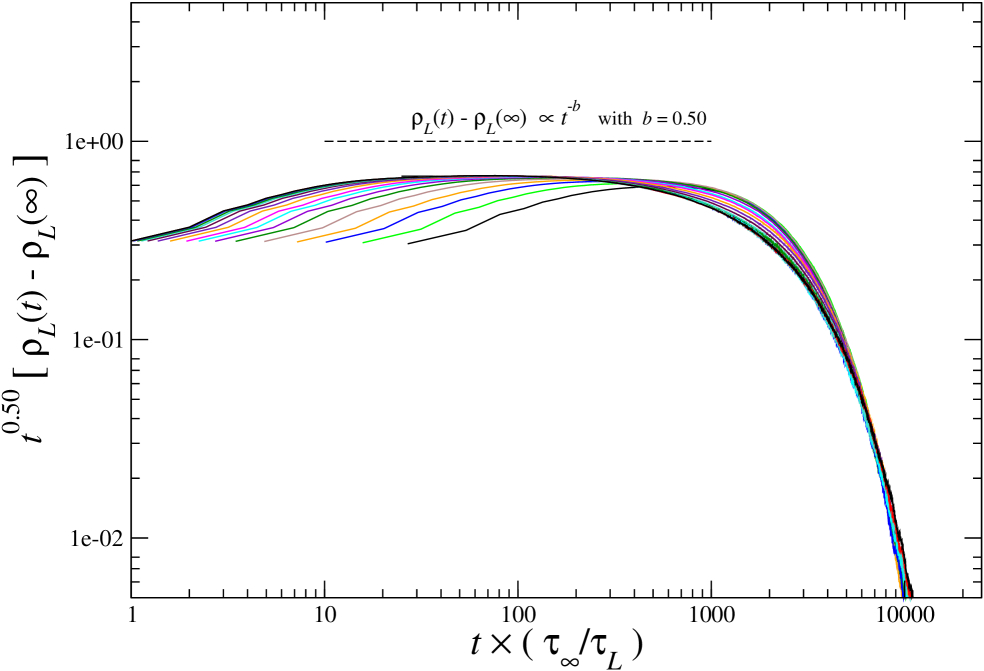
Figure 4: The curves of figure 1 multiplied by $t^{0.50}$ and with the time scaled such that their exponential tails coincide. The values of $L$ and the color code are as in figure 1. The power law regime appears as a plateau (dashed line).

We have simulated the time evolution of the GL on an $L\times L$ lattice for linear system sizes up to $L=512$. The system was started in a random initial configuration (“soup”) of density $\rho_{\rm in}=0.3$, meaning that each site was independently alive with probability $\rho_{\rm in}$ or dead with probability $1-\rho_{\rm in}$. We then observed the decay with time of the density $\rho_{L}(t)\equiv L^{-2}\sum_{{\bf{r}}}\langle n_{t}({\bf{r}})\rangle$, where the angular brackets $\langle\ldots\rangle$ stand for the average over the random initial configurations. Since we wish to analyze the decay of the density difference  $\rho_{L}(t)-\rho_{L}(\infty)$, which is analogous to an order parameter, we have in our simulations first determined the $L$ dependent quiescent state density $\rho_{L}(\infty)$.

2.1 Quiescent state density $\rho_{L}(\infty)$

Table 1 shows our simulation results for the quiescent state density $\rho_{L}(\infty)$ for system sizes from $L=128$ up, together with the number $N$ of quiescent states that contributed to each average. The error bars were obtained from the dispersion among ten subsets of quiescent states. The convergence to the infinite lattice limit $\rho^{*}\equiv\lim_{L\to\infty}\rho_{L}(\infty)$ seems to be at least exponential in $L$, but it is hard to ascertain its rate. The last line of table 1 lists what we feel is the best possible estimate,

$$\rho^{*}=0.02872\pm 0.00001,$$ (2.1)

which is compatible with, and slightly more accurate than, the best earlier determinations [21, 23].

2.2 Density decay at intermediate times

In figure 1, using now the values of the $\rho_{L}(\infty)$ determined above, we show in a log-log plot the decay curves of the density difference $\rho_{L}(t)-\rho_{L}(\infty)$ for various values of $L$. The most prominent feature is that in the large lattice limit the decay curves clearly converge to a limit curve $\rho(t)\equiv\lim_{L\to\infty}\rho_{L}(t)$. There appears to be an interval of almost two decades of intermediate times where the limit curve is close to linear, signaling a power law relation

$$\rho_{L}(t)-\rho_{L}(\infty)\propto t^{-b},\qquad 10\lesssim t\lesssim 1000.$$ (2.2)

The slope of the dashed straight line, drawn for comparison, shows that $b\approx 0.5$.

The steepening of the limit curve at times $t\gtrsim 2000$ indicates the crossover from power law to exponential decay. The GL is therefore subcritical: had it been critical, the power law would have held up to increasingly longer times for increasing $L$.

Bagnoli et al. [21] provide essentially the same limit curve, which they obtained for a lattice size of $320\times 200$ sites, but plot the density, instead of the density difference, as a function of time. For intermediate times such an analysis leads to a good linear fit $\rho(t)\propto t^{-\tilde{b}}$, but with a different exponent $\tilde{b}$ about equal to $\tilde{b}\approx 0.3$; Garcia et al. [24] in later work report $\tilde{b}=0.39\pm 0.04$. Neither work discusses the finite size behavior of this curve, which will be our next object of investigation.

2.3 Density decay for $t\to\infty$

Figure 1 shows that the smaller the lattice size $L$, the earlier the exponential decay sets in. We now proceed to discuss these finite size effects.

Figure 2 presents the same relaxation curves as figure 1, but in a log-linear plot which turns the exponential tails of the decay curves into straight lines. It appears that we have

$$\rho_{L}(t)-\rho_{L}(\infty)\propto{\rm e}^{-t/\tau_{L}}$$ (2.3)

without any extra multiplicative power of time on the RHS. Note that in figure 2 the differences $\rho_{L}(t)-\rho_{L}(\infty)$ go down to values as low as $10^{-6}$, as compared to only $10^{-3}$ in the time regime shown in figure 1. In figure 2 the intermediate power law decay has become nearly indistiguishable in the extreme upper left corner of the graph. The limiting curve is truly exponential only when $\rho(t)-\rho(\infty)$ is of the order of a few thousandths. In order that we obtain good statistics for such small density differences the curves for the largest values of $L$ required the largest computational effort (see table 1): those for $L\geq 144$ are averages over the time evolution of a number $N$ of initial configurations between $10\,000$ and $40\,000$. The curves for the smaller $L$ are averages over at least $100\,000$ initial configurations.

It is easy to extract the asymptotic decay time $\tau_{L}$ for each lattice size $L$ from the linear part of the corresponding decay curve. The $\tau_{L}$ are shown in a log-log plot in figure 3. For moderate $L$ they go up as a power law of $L$, but then saturate at a value $\tau_{\infty}\approx 1800$. Numerically we find

$$\tau_{L}\simeq\left\{\begin{array}[]{ll}AL^{z},&A=1.03,\quad z=1.66\pm 0.04,\\[5.69054pt] \tau_{\infty}=1800\pm 50,\phantom{XXX}&L\to\infty,\\ \end{array}\right.$$ (2.4)

where $z$ is the dynamical exponent. The individual error bars (not indicated) of each data point in figure 3 is chiefly due to the choice of the interval for the linear fit in figure 2. The small scatter in the set of data points is representative for these individual errors. The error bar $\pm 0.04$ in $z$ is due to the variations in slope of the red line still compatible with the data points. The error in $\tau_{\infty}$ is based on what seems a reasonable extrapolation.

Figure 3 shows that deviations from the power law first begin to occur, roughly, for $L\gtrsim 60$. We expect that this length scale also corresponds to a spatial correlation length and will investigate that idea in section 3.

For later reference we show in figure 4 the curves of figure 1 multiplied by the power $t^{b}$ (taking $b=0.50$) and with their time scaled by $\tau_{L}$. As a consequence, the power law regime appears as a plateau and the exponential tails coincide. In the regime of scaled times between roughly $500$ and $5000$ corrections to this finite size scaling are clearly visible; we have not investigated these any further.

3 Time dependent correlation length

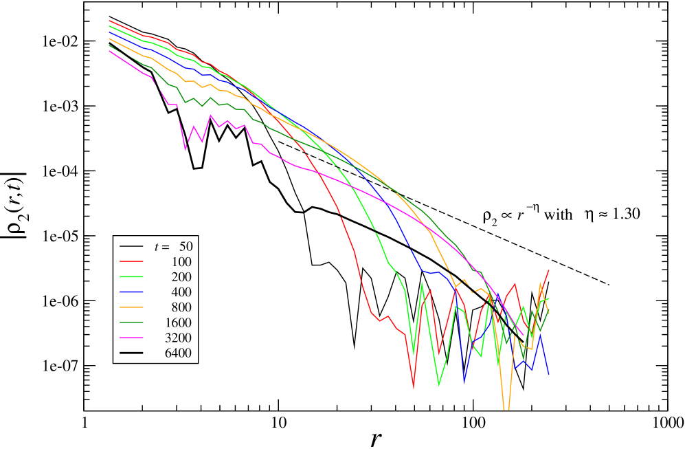
Figure 5: Truncated pair density $\rho_{2}(r,t)$ as a function of the radial distance $r$. The curves are for times $t=50,100,\ldots,6400$. All simulations are for a lattice of $512\times 512$ sites. The curves for the largest times, $t=3200$ and $t=6400$, are averages over $100\,000$ and $50\,000$ configurations, respectively. Those for the smaller times are each on $5000$ configurations. The dashed line has slope $-1.30$ and indicates the power law behavior discernible in an intermediate time regime of each curve before it steepens.

We wish to interpret the length scale identified above as a correlation length and to that end we now investigate the correlations between the occupation numbers on sites a distance $r$ apart. To the best of our knowledge, such correlations have not been studied before.

In the initial configuration the site occupation numbers of distinct sites are uncorrelated. For $t>0$ correlations will develop and we expect that there will be a time dependent correlation length $\xi_{t}$. The system being subcritical, this length must in the large time limit necessarily saturate at some finite constant value $\xi_{\infty}$.

For the simulations that follow we would ideally like to work on an infinite lattice. In practice we have worked on a $512\times 512$ lattice, whose linear size is considerably larger than the range of the expected correlations. We will conclude a posteriori  that for our purposes this lattice size is practically the “thermodynamic limit.”

We have determined the time dependent truncated pair density function

$$\rho_{2}(r,t)\equiv\langle n_{t}(0)n_{t}({\bf{r}})\rangle-\langle n_{t}(0)\rangle^{2}$$ (3.1)

where, as before, $\langle\ldots\rangle$ denotes the average over the random initial ensemble at density $\rho_{\rm in}=0.3$. The notation $\rho_{2}(r,t)$ in (3.1) is meant to include both a translational average and an average over the spatial annulus with $|{\bf{r}}|=r$.

Our interest is in the large $r$ behavior of the pair density and we have checked that circular symmetry sets in quickly for distances $\>\raisebox{-2.15277pt}{$\stackrel{{\scriptstyle\textstyle>}}{{\sim}}$}\>10$ lattice units. To represent $\rho_{2}(r,t)$ we divided the axis of the variable $\log r$ into equal-size bins centered at $r=r_{k}$ where $\log r_{k}=k/10$ for $k=0,1,2,\ldots$. This, combined with the annular average, leads to better statistics for large values of $r$. We have determined $\rho_{2}(r,t)$ for all $k$ such that $r_{k}\leq 180$. Figure 5 shows our raw data for the pair correlation $\rho_{2}(r,t)$, plotted as a function of $r$ for the geometric sequence of times $t=50,100,200,...,6400$. The figure first of all corroborates the expected phenomenon that the range of the correlations increases with time. It warrants numerous comments, that we will make in the four following subsections.

3.1 Correlation decay at intermediate and short distances

In an intermediate spatial range that depends on $t$ the curves show the power law behavior $\rho_{2}(r,t)\propto r^{-\eta}$ with $\eta=1.30\pm 0.10$. Although this intermediate range does not cover more than a decade, its existence again shows that the GL is not far from criticality.

The values of $\rho_{2}(r,t)$ for $r\lesssim 10$ represent short range correlations and are outside of our focus of attention, but we must nevertheless comment on them. The precise shape of $\rho_{2}(r,t)$ in this spatial region is definitely dependent on our choice of binning. The truncated pair density may, and in fact does have zeros on the $r$ axis. For $t=50$ a negative dip in the correlation occurs around $r=27$ and is followed by at least two further oscillations. As $t$ increases, this first dip moves to higher $r$, such that for $t=400$ it is located at $r=95$ and for $t=800$ it has moved out of the range of $r$ covered by our simulations. However, the existence of dips at larger $r$ may still reflect upon the $r$ dependence of the tail visible in the simulation.

For our longest times, $t=3200$ and $t=6400$, the short range structure in $\rho_{2}(r,t)$ is seen to strongly increase. We comment on this in subsection 3.3.

3.2 Correlation decay for $r\to\infty$

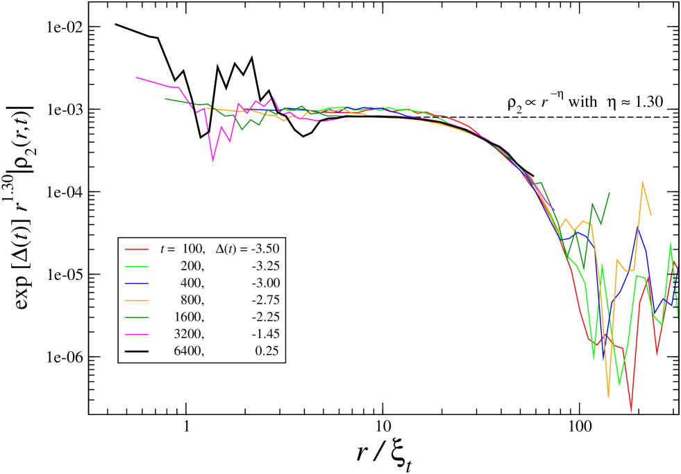
Figure 6: The curves of figure 5 multiplied by $r^{\eta}$ and shifted by $\Delta(t)$, as a function of the scaled coordinate $r/\xi_{t}$. This makes them coincide in the region $20\lesssim r/\xi_{t}\lesssim 80$ where their spatial decay begins to deviate from the power law $r^{-\eta}$.

Figure 6 shows a log-log plot of the data (except the $t=50$ curve) of figure 5 after they have been subjected to a scaling similar to, although more complicated than, the one that led to figure 4. The scaling here consists of the following three operations:

ii(i) Multiplication by the power $r^{1.30}$, which results in the power law regimes appearing as plateaus; the plateau is not very well developed at short times but becomes better visible at later times.

i(ii) Multiplication by a constant ${\rm e}^{\Delta(t)}$ chosen such that all plateaus are at the same common level indicated by the dashed line in the figure.
The “shift” $\Delta(t)$ is determined only up to a constant; we have arbitrarily set $\Delta(5600)=0$ (curve not shown). This shift describes the decay with time of the amplitude of the correlation. One might have expected that ${\rm e}^{-\Delta(t)}$ would be proportional to $\rho^{-2}(t)$, which in many cases in statistical physics is the natural normalization factor for the pair density; this simple normalization does not, however, appear to hold here. We find that for $400\lesssim t\lesssim 2400$ the shift $\Delta(t)$ is roughly linear in $t$.

(iii) Rescaling of the abscissa from $r$ to $r/\xi_{t}$, with the $\xi_{t}$ chosen such that for all curves their initial deviations from the plateau value occur at the same rescaled time. This determines the ratios of the $\xi_{t}$. We observe that there is a good scaling; its mathematically expression is

$$\rho_{2}(r,t)\simeq\frac{{\rm e}^{-\Delta(t)}}{r^{\eta}}\,{\cal G}\left(r/\xi_{t}\right),$$ (3.2)

valid in the time regimes of the power law and of its crossover to a steeper decay. It appears that in the region where the deviations from power law behavior first occur, i.e. for $20\lesssim r/\xi_{t}\lesssim 80$, the scaling function is best approximated not by an exponential but by ${\cal G}(u)=\mbox{cst}\times u\,{\rm e}^{-\kappa u}$. We have fixed the scale of the abscissa in figure 6 by the choice $\kappa=1$.

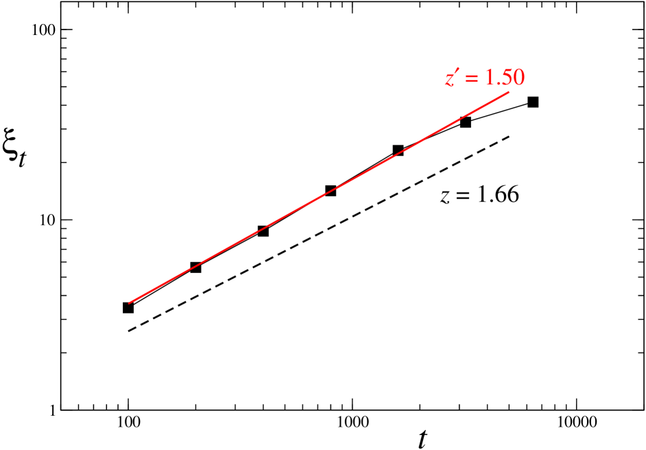
Figure 7: Data points: the correlation length $\xi_{t}$ as a function of time $t$ on a log-log scale. The red line is the best linear fit and has a slope $1/z^{\prime}$ with $z^{\prime}=1.50$, the dashed black line, shown for comparison, has slope $1/z$ with $z=1.66$ as determined in section 2.3.

The resulting values of $\xi_{t}$ are shown on a log-log scale in figure 7. Over most of the range shown there is a linear dependency, indicating the power law relation $\xi_{t}\propto t^{1/z^{\prime}}$. Deviations from this relation begin to occur only for $t=3200$ and become more apparent for $t=6400$. The saturation of $\xi_{t}$ at some finite value $\xi_{\infty}$, although only slow, seems clearly indicated; numerically we estimate

$$\xi_{t}\simeq\left\{\begin{array}[]{ll}B\,t^{1/z^{\prime}},&B=0.12,\qquad z^{\prime}=1.5\pm 0.1,\\[5.69054pt] \xi_{\infty}=50\pm 10,\phantom{XX}&t\to\infty.\end{array}\right.$$ (3.3)

Figure 7 shows for comparison also the straight line corresponding to the exponent value $z=1.66$ found in section 2. The two slopes are visually close to parallel, even though our estimates for the statistical errors in $z$ and $z^{\prime}$ fall short of overlapping.

The essence of our remarks below equation (2.4) about the error bar estimation remains valid here. In the absence of strong indications to the contrary, we adhere to the simplest scenario in which at each time $t$ there is only a single length scale, so that $z^{\prime}=z$. Our error bars reflect the statistical errors but do not take into account any systematic effects that there might be. We tentatively attribute the difference between the two values to a small but unknown systematic bias that we believe most likely affects the analysis of the correlation function, which is less straightforward than that of the density decay.

We note, finally, that the limit value $\xi_{\infty}$ in figure 7 cannot be estimated with the same accuracy as $\tau_{\infty}$ in figure 3.

3.3 Correlations upon the approach of the quiescent state

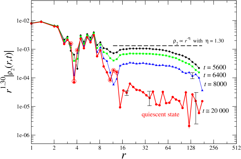
Figure 8: Truncated pair density function for four late times. The time $t=20\,000$ corresponds practically to the quiescent state. Error bars are discussed in the text; a few typical ones have been indicated. For the quiescent state (red curve) the six data points where $\rho_{2}$ is negative have been encircled. All runs were performed for lattice size $L=512$.

We now discuss the evolution of the pair correlation at late times, when the system approaches its quiescent state.

For the $512\times 512$ (essentially infinite) lattice the time decay of the density difference $\rho_{L}(t)-\rho_{L}(\infty)$ starts its crossover to exponential around $t\approx 1000$, but becomes truly exponential only for times as late as several thousand time units. The density $\rho_{L}(t)$ of living cells is then only a few thousandths above the quiescent state value $\rho^{*}=0.02872$.

The nature of the quiescent state has been recalled in the introduction. The small static and periodic objects of which it consists cannot overlap – if two of them were to overlap, they would interact and transform into something else. Therefore the constituents of the quiescent state act as “hard objects” with a typical diameter of the order of a few lattice units. This is a new short distance length scale, which changes the structure of the pair correlation.

Figure 8 shows the pair density (multiplied by the power law $r^{1.30}$) at four different times: $t=5600,\,6400,\,8000,$ and $20\,000$. The curves are averages over a number $N$ of independent systems equal to $N=35\,000,$  $50\,000,$  $20\,000,$ and $35\,000$, respectively. At time $t=20\,000$ (red curve) virtually all systems have reached the quiescent state.

All these runs were performed for lattice size $L=512$. Error bars were determined from the variance of ten subgroups of results. As expected, all error bars increase with $r$. For $t=5600$ and $t=6400$ they remain nevertheless at most of the order of the symbol size over the full range shown. For $t=8000$ they begin to considerably exceed the symbol size when $r\gtrsim 100$.

When the time $t$ is further increased, the curve $\rho_{2}(r,t)$ seemingly becomes a chaotic function of $r$. This appearance is due to two very different effects which we will discuss for $t=20\,000$.

i(i) First, for $r\lesssim 20$ the error bars in the $t=20\,000$ curve are still small, and what looks like a random curve is actually a reproducible structure, generated by the appearance of the new short range length scale. This is well illustrated by the phenomenon that we see happening near $r=12$ for late times. Near this point, the black and green curves begin to develop a dip that gradually deepens (blue curve). Beyond a certain time, $t\approx 9000$, the pair density at $r=12$ goes negative, as signaled by the encircled data points of the red curve.The associated oscillating behavior in space is analogous to that of the pair correlation in a dense liquid; in the present case the atoms are not the individual living cells, but the elementary static or periodic objects into which they have aggregated.

(ii) Secondly, for $r\gtrsim 20$, the randomness in the $t=20\,000$ curve is due to the difficulty of collecting good statistics. In this regime the error bars, some of which have been indicated, increase hugely with $r$ and this part of the curve is not reproducible. The root cause is again the aggregation of living cells into a few types of larger objects; this reduces the effective number of degrees of freedom without reducing the computational requirements, and hence makes averaging less efficient.

The question of whether the GL quiescent state is critical, i.e., has infinite correlation length, is of definite interest. It is from this state that Bak et al. [8] and later authors start in their attempts to show or disprove that the GL is self-organized critical. The present work provides strong indication that for $t\to\infty$ the GL correlation length $\xi_{t}$ tends to a finite  value $\xi_{\infty}$. The state of affairs described above makes clear, however, that it is very hard to track $\xi_{t}$ down in a simulation all the way to the quiescent state, or, in practice, to $t=20\,000$. We briefly return to related questions in section 5.

4 Decay time distribution

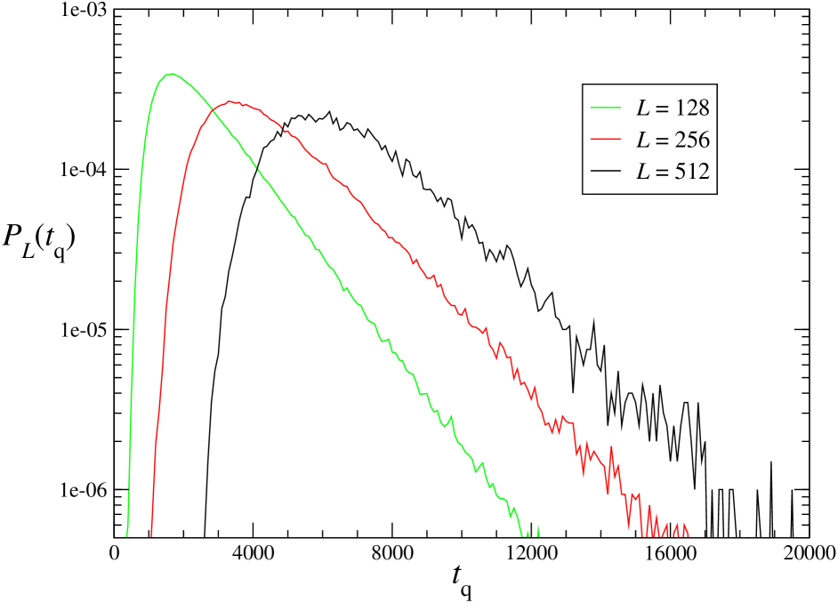
Figure 9: Probability distribution $P_{L}(t_{\rm q})$ of the decay time $t_{\rm q}$ to the quiescent state in systems of linear size $L=128,\,256$, and $512$. The exponential decay of the long time tail is manifest.

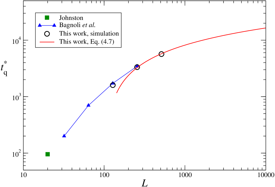
Figure 10: Time $t_{\rm q}^{*}$ for which $P_{L}(t)$ has a maximum, as a function of $L$. The square data point for $L=20$ is due to Johnston [25], the triangular ones for $L=32,\,64,\,128$, and $256$ are due to Bagnoli et al. [21] and have been connected to guide the eye, and the circular ones, for $L=128,\,256$, and $512$, were obtained in this work. The red line is the large $L$ expansion [equation (4.7)] of our heuristic theory.

Let $t_{\rm q}$ denote the random instant of time (the “decay time”) at which the system reaches its quiescent state. This random variable is of course determined by the random initial configuration and we will denote its distribution by $P_{L}(t_{\rm q})$. In this section we discuss how the dynamic exponent $z$ appears in this distribution.

4.1 Simulation data

For system sizes $L=128,\,256$, and $512$ we determined the distribution $P_{L}(t_{\rm q})$ from an ensemble of $900\,000$, $150\,000$, and $20\,000$ initial states, respectively. In figure 9 we present the resulting $P_{L}(t_{\rm q})$. Our results are fully consistent with the early work by Bagnoli et al. [21] for lattices of up to $L=256$, but present-day computational power allows for a much higher precision. It appears that the distribution has a “dead time” during which there is virtually zero probability for the system to reach its quiescent state, followed by a steep rise in this probability, which quickly attains a maximum. Finally, as is clear from figure 9, the curves decay exponentially for large times. It appears that the decay times (that we may call $\tau_{L}^{\prime}$) of the exponential tails are numerically indistinguishable from the $\tau_{L}$ obtained in figure 3. Hence we have from this simulation

$$P_{L}(t_{\rm q})\simeq a_{L}\,{\rm e}^{-t_{\rm q}/\tau_{L}},\qquad t_{\rm q}\to\infty,$$ (4.1)

with decay times $\tau_{L}$ as in equation (2.4).

Bagnoli et al. [21] considered the location $t_{\rm q}^{*}(L)$ where $P_{L}(t_{\rm q})$ peaks and found that in the regime of system sizes they studied it may be described by a power law $t_{\rm q}^{*}(L)\propto L^{\zeta}$ with $\zeta\approx 0.7$ (they denote this $\zeta$ by $z$). In figure 10 we show their data points, as well as our own, for $L=128,\,256$, and $512$. For $L=128$ and $L=256$ our values are seen to virtually coincide with those of Ref. [21]. The data, however, suggest a downward curvature, which is reinforced by our data point at $L=512$. We investigate the large $L$ behavior of this curve in the next subsection.

4.2 Heuristic argument

We construct here for the curve $t_{\rm q}^{*}(L)$ of figure 10 a heuristic argument valid in the limit of asymptotically large $L$, which in practice is attained when $L\gtrsim\xi_{\infty}$. In that limit we expect $t_{\rm q}^{*}(L)$ also to tend to infinity.

At a given time $t$, let us imagine an $L\times L$ lattice divided up into $L^{2}/\xi_{t}^{2}$ blocks of size $\xi_{t}\times\xi_{t}$. Such blocks may be considered as statistically independent, due to not yet having had enough time to interact. Let the function $c_{L}(t)$ indicate the probability at time $t$ that a $\xi_{t}\times\xi_{t}$ block be quiescent. This function is unknown but we certainly expect it to increase with time and be such that $c_{L}(\infty)=1$. Let $Q_{L}(t)$ be the probability at time $t$ that an $L\times L$ system be quiescent. For this to be true, it is necessary that all its $\xi_{t}\times\xi_{t}$ blocks be quiescent, and therefore

$$Q_{L}(t)=c_{L}(t)^{L^{2}/\xi_{t}^{2}}.$$ (4.2)

Whereas mathematically $c_{L}(t)$ and $Q_{L}(t)$ are equivalent, the tacit assumption here is that $c_{L}(t)$ is only weakly $L$ dependent, and that we may exploit this feature.

In practice it is more convenient to work with the function $f_{L}(t)$ defined by

$$Q_{L}(t)={\rm e}^{-L^{2}f_{L}(t)},\qquad f_{L}(t)=\frac{1}{\xi_{t}^{2}}\log\frac{1}{c_{L}(t)}\,,$$ (4.3)

and which is also expected to be only weakly $L$ dependent. Since $c_{L}(t)\to 1$ for $t\to\infty$, we have that $f_{L}(t)\to 0$ in that limit.

Using that $P_{L}(t)=(\mbox{d}/\mbox{d}t)\,Q_{L}(t)$ we get from equation (4.3) the expression

$$P_{L}(t)=-L^{2}f^{\prime}_{L}(t){\rm e}^{-L^{2}f_{L}(t)}.$$ (4.4)

The maximum of $P_{L}(t)$ is the solution of $(\mbox{d}/\mbox{d}t)P_{L}(t)|_{t=t_{\rm q}^{*}}=0$, which gives

$$f_{L}^{\prime\prime}(t_{\rm q}^{*})=L^{2}f_{L}^{\prime 2}(t_{\rm q}^{*}).$$ (4.5)

We compare (4.4) to the findings of our simulation, namely equation (4.1), and obtain after a time integration

$$f_{L}(t)=-\frac{1}{L^{2}}\,\log(1-a_{L}\tau_{L}{\rm e}^{-t/\tau_{L}}),\qquad L\gg\xi_{\infty}\,.$$ (4.6)

In the large $L$ limit $\tau_{L}$ tends to $\tau_{\infty}\approx 1800$, and it appears from the simulation that the ratio $a_{L}/L^{2}$ tends to the fixed value $a_{L}/L^{2}\equiv A\approx 5.2\times 10^{-8}$. Upon inserting (4.6) in the maximum condition (4.5) we obtain

$$t_{\rm q}^{*}(L)=2\tau_{\infty}\log L\,+\,\tau_{\infty}\log A\tau_{\infty}\,.$$ (4.7)

This curve, with the values of $A$ and $\tau_{\infty}$ as stated before, has been presented as the solid red line in figure 10. We see that for $L\gtrsim 256$ it is in excellent agreement with the two data points and provides a credible asymptotic expression for larger $L$.

It should be noted, however, that this is a lowest order approximation, based on the empirical input formula (4.1). We have not pursued the possibility of improving the result by adding higher order correction terms to that formula.

5 Discussion

We have considered the statistics of the Game of Life (GL) on an $L\times L$ square lattice for sizes up to $L=512$. Even though we used no special programming techniques, our accuracy is higher than that of earlier work, which mostly dates back one or two decades.

We have studied finite size effects and established the dependence of the asymptotic density relaxation time $\tau_{L}$ on the system size $L$. We found that in an intermediate range of system sizes $\tau_{L}\propto L^{z}$ with a dynamical exponent $z=1.66\pm 0.04$; and that for system sizes $L\gtrsim 180$ the relaxation time $\tau_{L}$ saturates and approaches the constant value $\tau_{\infty}=1800\pm 50$, independent of system size.

We have performed the first study, to the best of our knowledge, of correlation functions in the GL. We found that when the system relaxes from a random initial state, the large distance decay of the pair density may be characterized by a time dependent correlation length $\xi_{t}$. We found that for an intermediate range of times $\xi_{t}\propto t^{1/z^{\prime}}$ with $z^{\prime}$ close to $z$, whereas for times $t\gtrsim 6000$ there is saturation at a constant value $\xi_{\infty}=50\pm 10$.

Hence there are lattice size independent cutoffs in space and time, exactly as one would expect for a noncritical system. Larger lattices have been considered by several investigators in the past, but sizes larger than $L=512$ are not needed to reach our conclusions.

We briefly add a few more comments on the relation between our results and other work that has been reported in the literature.

Bennett and Bourzutschky [17] obtain a correlation length of $42\pm 3$ lattice distances, which compares favorably with our $\xi_{\infty}=50\pm 10$. Their value is based, essentially, on the penetration length of the density into the system away from a boundary of cells kept alive randomly; we have independently confirmed [26] the length obtained by such a procedure. The relaxation time of $200\pm 10$ time steps reported by same authors [17] is an average  time and refers to the relaxation of external perturbations; it cannot be compared to the asymptotic time $\tau_{\infty}$ of present work.

We have not explored initial densities other than the value $\rho_{\rm in}=0.3$. It appears in simulations [21, 27, 24, 16] that there is an interval $0.15\lesssim\rho_{\rm in}\lesssim 0.75$ for which the density $\rho^{*}$ of the final quiescent state is constant within the accuracy of the simulation. Gibbs and Stauffer [23], in particular, starting from an initial density $\rho_{\rm in}=0.5$, obtained the same quiescent state density $\rho^{*}$ of our equation (2.1) to within at least three decimals of accuracy. The curves $\rho_{L}(t)$ for different initial densities approach each other rapidly (as it seems, exponentially fast in time). This does not prove, but at least suggests, that the exponents associated with this decay are universal with respect to $\rho_{\rm in}$ within the interval in question. We therefore speculate that the asymptotic relation between the length and time scales found in the present work for $\rho_{\rm in}=0.3$ in fact holds in this whole interval of initial densities.

The question of universality may be asked also about the exponents $b$ (for the density; section 2.2) and $\eta$ (for the correlation function; section 3.1). Whereas $z$ and $z^{\prime}$ concern the asymptotic exponential decay (of the density in time, and of the correlation function in space, respectively), the exponents $b$ and $\eta$ refer to intermediate power law regimes. Speculation, therefore, seems more dangerous here. We have no data on $\eta$ for initial densities other than $\rho_{\rm in}=0.30$. As far as $b$ is concerned, simulation of the density decay for different initial densities shows that for $\rho_{\rm in}\lesssim 0.25$ and $\rho_{\rm in}\gtrsim 0.50$ the power law regime becomes too ill-defined to extract an exponent $b$; but that within these limit values there is no obvious variation of $b$ with $\rho_{\rm in}$.

We believe that the various questions touched upon in this discussion leave much room for future research.

References

- [1] E.R. Berlekamp, J.H. Conway, and R.K. Guy, Winning Ways for Your Mathematical Plays Vol. 2 (Academic Press, New York 1982).
- [2] M. Gardner, Scientific American 223 (4) 120; 223 (5) 118; 223 (6) 114 (1970).
- [3] S. Wolfram, Physica D 10 (1984) 1.
- [4] S. Wolfram and N.H. Packard, J. Stat. Phys. 38 (1985) 901.
- [5] D. Eppstein in Game of Life Cellular Automata, Ed. A. Adamatzky (Springer, London, 2010), p. 71.
- [6] M. Dresden and D. Wong, Proc. Nat. Acad. Sci. 72 (1975) 956.
- [7] L.S. Schulman and P.E. Seiden, J. Stat. Phys. 19 (1978) 293.
- [8] P. Bak, K. Chen, and M. Creutz, Nature 342 (1989) 780.
- [9] P. Bak, C. Tang, and K. Wiesenfeld, Phys. Rev. Lett. 59 (1987) 381.
- [10] M. Creutz, Nuclear Physics B (Proc. Suppl.) 26 (1992) 252.
- [11] P. Bak, Physica A 191 (1992) 41.
- [12] P. Alstrøm and J. Leão, Phys. Rev. E 49 (1994) R2507.
- [13] M. Creutz in Some New Directions in Science on Computers, Eds. De Gyan Bhanot, Shiyi Chen, and Philip Seiden (World Scientific, 1997), p. 147.
- [14] K.M. Fehsenfeld, M.A.F. Gomes, and T.R.M. Sales, J. Phys. A 31 (1998) 8417.
- [15] D.L. Turcotte, Rep. Progr. Phys. 62 (1999) 1377.
- [16] A.F. Rozenfeld, K. Laneri, and E.V. Albano, Eur. Phys. J. Special Topics 143 (2007) 3.
- [17] C. Bennett and M.S. Bourzutschky, Nature 350 (1991) 468.
- [18] J. Hemmingsson, Physica D 80 (1995) 151.
- [19] J. Nordfalk and P. Alstrøm, Phys. Rev. E 54 (1996) R1025.
- [20] H.J. Blok and B. Birgersen, Phys. Rev. E 55 (1997) 6249.
- [21] F. Bagnoli, R. Rechtman, and S. Ruffo, Physica A 171 (1991) 249.
-
[22]
http://web.stanford.edu/cdebs/GameOfLife/
http://wwwhomes.uni-bielefeld.de/achim/gol.html
http://www.math.com/students/wonders/life/life.html - [23] P. Gibbs and D. Stauffer, Int. J. Mod. Phys. C 8 (1997) 601.
- [24] J.B.C. Garcia, M.A.F. Gomes, T.I. Jyh, T.I. Ren, and T.R.M. Sales, Phys. Rev. E 48 (1993) 3345.
-
[25]
N. Johnston,
http://www.njohnston.ca/2009/07/the-maximal-lifespan-
of-patterns-in-conways-game-of-life/ - [26] F. Cornu and H.J. Hilhorst, unpunblished.
- [27] K. Malarz, K. Kulakowski, M. Antionuk, M. Grodecki, and D. Stauffer, Int. J. Mod. Phys. C 9 (1998) 449.