Generating Artificial Reference Images for Open Loop Correlation Wavefront Sensors

Abstract

Shack-Hartmann wavefront sensors for both solar and laser guide star adaptive optics (with elongated spots) need to observe extended objects. Correlation techniques have been successfully employed to measure the wavefront gradient in solar adaptive optics systems and have been proposed for laser guide star systems. In this paper we describe a method for synthesising reference images for correlation Shack-Hartmann wavefront sensors with a larger field of view than individual sub-apertures. We then show how these supersized reference images can increase the performance of correlation wavefront sensors in regimes where large relative shifts are induced between sub-apertures, such as those observed in open-loop wavefront sensors. The technique we describe requires no external knowledge outside of the wavefront-sensor images, making it available as an entirely “software” upgrade to an existing adaptive optics system. For solar adaptive optics we show the supersized reference images extend the magnitude of shifts which can be accurately measured from $12\%$ to $50\%$ of the field of view of a sub-aperture and in laser guide star wavefront sensors the magnitude of centroids that can be accurately measured is increased from $12\%$ to $25\%$ of the total field of view of the sub-aperture.

1 Introduction

Adaptive optics (AO) is integral to all next generation solar and Extremely Large Telescope (ELT) class ground based telescopes, including the European solar telescope (EST) (Collados et al., 2013) and the ELT (Davies et al., 2010; Cuby et al., 2010). These telescopes will employ complex AO systems which use tomography and multiple deformable mirrors in order to increase either the corrected field of view (FOV) using multi-conjugate adaptive optics (MCAO) modalities (Davies et al., 2010), or the number of corrected targets ( multi-object adaptive optics (MOAO)) (Cuby et al., 2010).

Extended objects are currently the only source available for wave-front sensors in solar AO (typically solar granulation) and are also present on ELTs due to laser guide star (LGS) elongation. The impact of LGS elongation on AO is the subject of ongoing studies(Thomas et al., 2008; Conan et al., 2009; Gilles & Ellerbroek, 2006; Schreiber et al., 2010; Anugu et al., 2018). Furthermore, the available WFS camera options for first light ELT instruments impose restrictions on the available FOV resulting in truncation, or limited sampling, of the LGS plume. Similarly, for solar AO the effect of how to best use and analyse extended sources in WFSs is the subject of similar studies (Löfdahl, 2010). One solution to the problem of measuring centroids on extended structure for solar AO, proposed by Rimmele & von der Luehe (1990), is the use of correlations in order to accurately measure centroids when observing extended structures. This technique has been employed successfully in a number of solar AO systems, including the Swedish solar telescope (SST) (Scharmer et al., 2002), GREGOR (Soltau et al., 2013) and the new solar telescope (NST) (Cao et al., 2010) and has also been shown to improve LGS WFSs on-sky (Basden et al., 2014).

Correlation technniques are subject to the same noise sources as other centroiding techniques, including all of the noise sources associated with electrical and optical noise. However, there is also another source of noise which correlation techniques are subject to, which most other techniques are not. This extra noise is due to different structure being present in the reference and sub-aperture images which are cross-correlated. This noise term is a source of model error, and in the rest of the paper referred to as model error. Model error is especially relevant in open-loop AO systems, whose WFSs observe the full strength of atmospheric turbulence, not just residuals after a correction has been applied to the wavefront, as is the case for closed loop WFSs.

In this paper we propose a computational solution to model error which employs the use of multiple sub-apertures to generate a “supersized” reference image. This supersized reference image can then be used as the reference image in cross-correlations to reduce the model error, as well as other effects which arise from noise in the reference image. This is shown to improve centoriding accuracy via simulation and allow reliable centroiding for a magnitude of sub-aperture shifts which previously could not be measured.

In order to minimise error sources which are not due to model error the technique described in Townson et al. (2015) was used in order to choose optimal centroiding parameters for estimating the centre of mass (COM) of the correlation images. The simulations were also run in noiseless conditions to only show the effects of model error.

2 Model Error

Model Error is defined here to be noise sources which arise in correlation images from structure which is not present in both the reference and sub-aperture images, this is also referred to as “truncation” for LGSs in night-time AO. An illustration of this is given in Fig. 1.

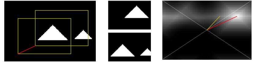
Figure 1: The left part of the figure shows a large, extended, FOV which is sampled by a WFS. The yellow rectangles show the FOVs of a single sub-aperture and a reference sub-aperture. The red line shows the shift between the two images. The middle section of the figure shows the sub-aperture image and the reference image individually. It can be seen that the sub-aperture image has structure which is not present in the reference image. The right part of the figure shows the correlation image from calculating the cross-correlation between the reference image and sub-aperture image. The original shift is shown in red and the measured centroid is shown in yellow. The centroid is displaced from the true image shift by the extra structure present only in the sub-aperture image.

We expect the centroid measurement to correspond to the shift between the sub-aperture image and the reference image. Here the model error can be seen to add a strong signal to the correlation image, which then skews the centroid measurement away from the value of the shift between the two images. The left panel shows the “full” FOV, with the two yellow boxes showing the FOVs of the reference image and the sub-aperture image. The red line indicates the shift between the reference and the sub-aperture image. In the middle panel the reference and sub-aperture images are individually displayed, it can be seen that there is an additional structure in the sub-aperture image which is not present in the reference image. The right panel shows the resulting correlation image from cross-correlating the reference and sub-aperture images. The red line shows the shift between the two images and the yellow line shows the measured centroid of the correlation image. The difference between the centroid and the true image shift is due to model error, and arises from the structure in the correlation image created from the non-common elements between the reference and sub-aperture images. This shifts the centroid estimate towards it and away from the actual value.

The example shown in Fig. 1 shows a highly simplified case where there are only two structure in the whole field. For solar granulation there is structure distributed continuously in all directions, this manifests itself as a high background in the correlation image, with many small peaks distributed across it. In LGS images there is continuous structure along the direction of the laser plume. Although centroiding correlation images which display structure unrelated to the overlap of content common to both images can add noise to the centroid measured there are methods which attempt to minimise the influence of this erroneous structure, such as Townson et al. (2015); Löfdahl (2010). These methods make use of windows and threshold values around the peak of the correlation image to remove the influence of non-common structure.

However, while these methods minimise some of the effects of model error they make no attempt to remove it, leaving it present in the correlation images and still making a contribution to the error in any centroid measurement. Also, for large shifts between sub-aperture and reference images, the overlap region where the peak of the correlation signal is generated is reduced compared to a small shift. This reduction in the area of overlap for the peak of the correlation image increases the noise on the signal in the correlation image, which in turn adds noise to centroids on the correlation image. These effects increase when the relative shift between sub-aperture image and the reference image increases, making the problem greater for open-loop WFSs.

3 Minimising Model Error

We suggest that the structure in every sub-aperture image should be wholly contained in the reference image, this should remove the effect of model error. Sub-aperture images sample different FOVs due to atmospheric turbulence perturbing the path of incoming wavefronts (Roddier, 1981; Shack & Platt, 1971). By combining a set of sub-aperture images, either from a single WFS frame or a temporal sample, a larger FOV can be reconstructed than the FOV contained in any individual sub-aperture image. This larger image now samples the full FOV which all parts of the WFS observe. This generated image can be used as the reference image for correlation WFSing and provide a reference image which includes completely the smaller individual sub-apertures. The supersized reference image can be used with subsequent frames of a WFS, so long as the structure of images in the FOV observed remains unchanged.

Each pixel in the generated reference image will be the result of combining multiple sub-aperture images, reducing noise (Basden et al., 2014). However, for the purposes of this paper we concentrate on the model error aspect of synthesising supersized reference images, especially addressing the “chicken and egg” problem of requiring good image shift measurements in order to generate a supersized reference image which in turn is required to measure image shifts.

Figure 2 illustrates the effect of using a supersized reference image in a correlating WFS in a similar layout to Fig. 1.

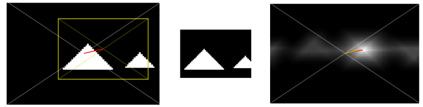
Figure 2: Similarly to Fig. 1 the left part shows a large FOV, with the yellow box highlighting the FOV of a single sub-aperture. The middle region shows just the sub-aperture image, as the reference image is taken to be the full FOV shown in the left part of the figure. The right part shows the correlation image from a cross-correlation of the sub-aperture image with the full FOV. The red line indicates the shift of the sub-aperture and the yellow line shows the measured centroid of the correlation image. There is still a discrepancy between the shift and the centroid measurement, however, this difference is greatly reduced compared to Fig. 1.

Here the full field is used as the reference image, so only one sub-aperture FOV is highlighted with a yellow window. When this sub-aperture is correlated with the full field the resulting correlation image shows similar features to Fig. 1, but the peak of the correlation is much stronger, so the similar structure which adds features to the correlation image have less of an impact on the centroid measurement than it did for Fig. 1. This can be seen through the red and yellow lines overlaid on the correlation image, which correspond to the image shift and centroid measurement respectively. The lines are much closer than they were in Fig. 1, showing the centroid is more accurate. The correlation from the overlap of the larger and smaller triangles is still in the correlation image, biasing the centroid measurement, but it has a reduced effect compared to Fig. 1.

In the next section we go on to describe a method to generate supersized reference images using WFS data, and show results from simulation on both solar granulation and LGS WFS images. However, in order to generate a supersized reference image a set of sub-aperture images must be centroided. This can be an issue in open-loop correlation WFSs and generally for correlation WFSs before the AO loop is closed. Below we describe a method for overcoming this issue.

3.1 Measuring Large Relative Image Shifts

In regimes where the relative shifts between sub-aperture images and reference images is a significant fraction of the FOV of the sub-aperture correlation wavefront sensing fails. Using a supersized reference image can allow for shifts of this magnitude to be accurately measured, however, there is an issue in generating a supersized reference image in this regime where traditional correlation wavefront sensing fails. Also, the centroiding parameters used to measure the location of the peak of a correlation image can add noise to the measured centroids. To minimise noise arising from centroiding parameters we estimate the optimal window and threshold values for a centre of mass on the correlation images using Townson et al. (2015).

Whilst large image shifts exist between some sub-apertures in any particular WFS frame, adjacent sub-apertures usually have small relative shifts due to the continuous structure of turbulence. Indeed, for any chosen sub-aperture in a WFS frame there will be a number of other sub-apertures with similar absolute shifts. Figure 3 shows the absolute shift of each sub-aperture for an $r_{0}$ of $10$\mathrm{cm}$$ in the upper histogram. The lower histogram in Fig. 3 shows the smallest relative shift between each sub-aperture and its closest neighbour for a WFS in the same conditions.

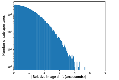
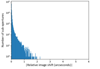
Figure 3: The upper plot shows the distribution in shifts of sub-apertures in a WFS for an $r_{0}$ of $0.10$\mathrm{m}$$. For a typical open-loop solar WFS, shifts larger than $1$\mathrm{\SIUnitSymbolArcsecond}$$ are difficult to measure accurately, leaving a significant number of sub-apertures without a reliable centroid. However, there is nearly always another sub-aperture within this range in the WFS. The lower plot shows the absolute smallest relative shift for all sub-apertures in a WFS. Here there are significantly more pairs of sub-apertures with small relative shifts and a small fraction which have relative shifts above $1$\mathrm{\SIUnitSymbolArcsecond}$$.

If we use a pixel scale of $0.25$\mathrm{\SIUnitSymbolArcsecond}$/\textrm{pixel}$, and a sub-aperture size of 16 pixels, then a shift of $1$\mathrm{\SIUnitSymbolArcsecond}$$ will be the limit of what can be reliably centroided using a traditional correlation, corresponding to roughly $25\%$ of a sub-aperture width. However, by choosing the reference sub-aperture individually for every sub-aperture in the WFS the measured shift can be minimised, reducing the magnitude of shifts measured from the upper part of Fig. 3 to that shown in the lower part. The individual relative measurements can then be “tiled” across the WFS frame and combined to generate the absolute shift of each sub-aperture as shown in Fig. 4(b). The relative shift between sub-aperture $S$ and $R$ in Fig. 4(a) is likely to be large as the sub-apertures have a large physical separation, meaning the measured centroid is likely to have a large error. In Fig. 4(b) the relative shift between sub-aperture $S$ and sub-aperture $R$ can be found by summing the relative shifts between between adjacent sub-apertures, as depicted by the red dotted line. There are many different combinations of sub-apertures that could be combined to calculate the relative shift between $S$ and $R$, giving many estimates of the shift. These can be combined to reduce the error on the shift measurement. This method can be extended to the full WFS frame, using a combination of all pairs of sub-apertures to generate correlation images then fitting the individual sub-aperture shifts and using a least squares type.

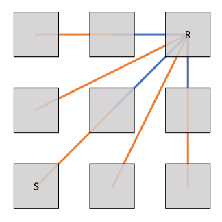
(a) Single reference image

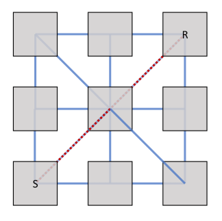
(b) Tiling reference images

Figure 4: A $3\times 3$ grid of sub-apertures with cross-correlations shown for a single reference image 4(a) and using all pairs of sub-apertures 4(b). In 4(a) we see three “good” cross-correlations, shown in blue, where the sub-apertures are adjacent and have relatively small shifts. We also see “bad” cross-correlations in orange. These are drawn for sub-apertures which are not adjacent to the reference image, where the model noise is likely to be larger. 4(b) shows only the adjacent sub-aperture pairs which are cross-correlated using the ‘tiling’ method. Whilst there are still many pairs of sub-apertures which are considered to be “bad” there are also many which are “good”. Every sub-aperture in the WFS frame can be cross-correlated using only “good”, blue, cross-correlations. The absolute shift of each sub-aperture can then can be determined using only information contained in the cross-correlations from adjacent pairs of sub-apertures.

Using a least square fit, which includes every possible pair of sub-apertures in a WFS frame, to estimate the centroids of a set of sub-aperture images mandates every pair of sub-apertures is cross-correlated. While this includes the pairs of sub-apertures with large relative shifts, it also includes all of the larger number of pairs with small relative shifts which can be accurately centroided. This process can be further optimised by adding a weighting function in the least squares fit. Centroid measurements which are large can be given a low weighting, and small measures given a greater weighting. This suppresses the contribution of pairs of sub-apertures with large measured relative shifts, as these are known to include a larger model error. This leaves us with the least squares problem of the form described in Eqn. 1;

$$\left(\begin{array}[]{ccc}w^{0,1}&-w^{0,1}\\ w^{0,2}&&-w^{0,2}\\ &w^{1,2}&-w^{1,2}\end{array}\right)\left(\begin{array}[]{c}\mathbf{R}^{0}\\ \mathbf{R}^{1}\\ \mathbf{R}^{2}\end{array}\right)=\left(\begin{array}[]{ccc}w^{0,1}\\ w^{0,2}\\ w^{1,2}\end{array}\right)\left(\begin{array}[]{ccc}\mathbf{R}^{0,1}\\ \mathbf{R}^{0,2}\\ \mathbf{R}^{1,2}\end{array}\right)^{T},$$ (1)

where $w^{i,j}$ is the weight applied to the centroid of sub-aperture $i$ cross-correlated with sub-aperture $j$, $\mathbf{R}^{i}$ is the absolute shift of sub-aperture $i$ and $\mathbf{R}^{i,j}$ is the relative shift between sub-apertures $i$ and $j$. The values of $\mathbf{R}^{i,j}$ are measured by centroiding the correlation image between the sub-apertures and the weights applied are the inverse of the magnitude of these centroids, such that;

$$w^{i,j}=\frac{1}{|\mathbf{R}^{i,j}|}.$$ (2)

There are other metrics which could be used as a weighting variable for the least squares fit, such as the contrast or sharpness of the individual sub-aperture images or the residuals from a unitary weighted fit. However, using the magnitude of the measured shift is a natural solution to the problem we are trying to solve in that it suppresses the measurements which experience the largest model error. On real AO systems there may be other noise effects which mean a different choice of weighting function would be more appropriate.

3.2 Reference Image Generation

Using the technique described in the Sec. 3.1 a series of sub-aperture images, with large relative shifts, from a WFS can have their individual image shifts measured. The simplest way to synthesise a reference image from WFS images and image shift measurements is to align the individual images using the shift measurements and sum them. This has been implemented before by Basden et al. (2014), where the technique is used to increase the signal to noise ratio (SNR) of the reference image for LGS. However, by keeping all parts of the aligned image rather than cropping to the FOV of a sub-aperture, we can create a supersized reference image. This has the effect of reducing noise in the reference image, in a similar way to Basden et al. (2014), but also offers a solution to model error.

By using all sub-apertures in a WFS frame a supersized reference image can be created which contains no regions which are not sampled by at least one sub-aperture image. The fill factor can be increased further if multiple frames are used together to create a supersized reference iamge. However, the edges of the supersized reference image can still be under-sampled if there are too few sub-aperture images with large absolute shifts.

Here, to create supersized reference images initially the sub-aperture images were up-sampled to $10\times$ their original size, to enable alignment of the images to a sub-pixel scale. The images were then stacked, rounding the shifts to the nearest tenth of a pixel, so the shifts were all an integer number of pixels on the up-sampled sub-aperture images. All parts of the images were kept after the alignment, such that the resulting stacked image had a larger FOV than the original FOV in the sub-aperture images. Although Fast Fourier Transform (FFT) methods exist for co-aligning images, these were not employed as they typically do not allow for a larger sized output image than input. This super-sized image was then binned back down to the original scale of the WFS, generating an image similar to the input sub-aperture images, but with higher SNR and a larger FOV. Example synthesised supersized reference images from simulated solar and LGS WFS images are shown in Fig. 5. The LGS image contains elongation which is representative of those expected to be observed at the edge of the ELT pupil.

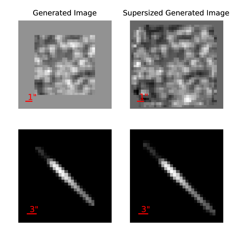
Figure 5: Images of generated reference images shown beside supersized reference images. The upper images show the case for images of solar granulation and the lower images show the case for images of elongated LGSs, shown on a logarithmic scale to highlight the edges of the laser plume. The left images show the full FOV observed by a single sub-aperture and the right images show the full synthesised supersized reference images. The scale of the sub-aperture and supersized reference images is the same for each object, with the padding showing the areas where extra information present in the supersized reference images.

The initial supersized reference images which are created from using the centroids from the least squares fit described in Sec. 3.1 are not always sufficient be used as reference images for cross-correlation. This is due to the accuracy of the centroid measurements which arise from the least squares technique. However, the synthesised supersized reference image does contain a larger FOV and show the structure found in the sub-aperture images, so can be used in order to estimate the shifts of the same set of sub-apertures again, to a higher accuracy. This process can then be repeated, in a bootstrap type method, multiple times in order to “refine” the synthesised supersized reference image. After a certain number of iterations the centroid estimates will no longer change from each iteration, so the generated supersized reference image stabilises. This occurs when the centroids from the sub-apertures is optimal, so the synthesised reference image is also optimal for the input set of sub-aperture images. This supersized reference image can then be used as the reference image to measure the centroids in subsequent WFS frames.

Due to the distribution of shifts in Fig. 3 the edges of the supersized image is contained in relatively few of the sub-aperture images. The resulting SNR in a supersized reference image therefore varies across the supersized image. In the centre of the image the SNR is highest and it decreases further from the centre. The resulting shift estimates from using a supersized reference image will therefore be more reliable for small shifts and less reliable for large shifts, where the edges of the supersized reference images contribute signal to the cross-correlation. This effect can be reduced by using more sub-aperture images, from different frames, to generate a supersized reference image. Though the estimates from a supersized reference image with poor SNR at the edges of the FOV will be more accurate than if there was no structure in the reference image i.e. the reference image had a smaller FOV. This effect of differential noise properties across the supersized reference image is not investigated here, as noiseless images are used in the simulations to only show the effect of model error.

4 Comparison of Reference Images

The technique described in Sec. 3 was compared with the widely used method of using a single sub-aperture image as the reference image in correlation WFSing. WFS images of solar granulation and LGSs were simulated with relative shifts representative of Von-Karman atmospheric turbulence, and centroided by cross-correlating them with a single, central un-vignetted sub-aperture as the reference image in order to obtain a baseline performance for the standard method of performing correlation WFSing. The least squares method of measuring centroids, described in Sec. 3.1 was performed and its root mean square (rms) error measured, along with the rms error from using synthesised reference images generated from the WFS image. The synthesised reference images were used in two situations, the first where the supersized reference image was windowed to the original FOV of a single sub-aperture, comparable to the method used in Basden et al. (2014), and the second where the full FOV of the supersized reference image was used. The results for both sub-aperture images of solar granulation and highly elongated LGS images are shown in Fig. 6.

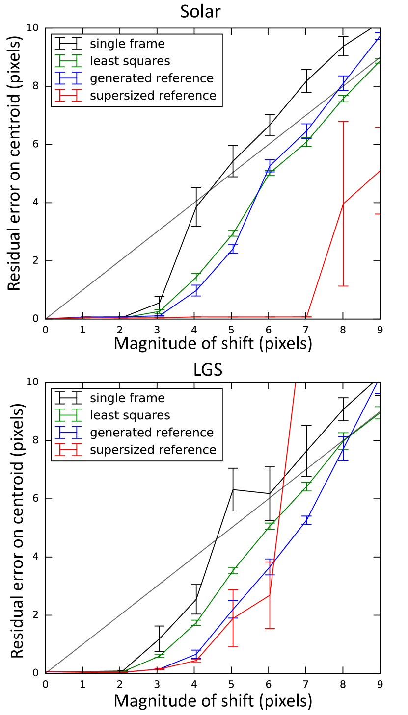
Figure 6: The upper figure shows the results of the various correlation centroiding techniques on images of solar granulation and the lower plot shows the same techniques applied to highly elongated LGS images. The black line shows the residual error from using a single sub-aperture image as the reference image in a cross-correlation. The green line shows the performance of the least squares technique described in sec. 3.1, the blue line shows the performance of a synthesised reference image windowed to the same FOV as a single sub-aperture and the red line shows the performance of the full supersized reference image. The grey line shows $y=x$ for reference of centroiding accuracy. All centroiding methods perform similarly, better than 0.1 pixels, for shifts of less than 3 pixels.

Using a single sub-aperture as the reference image works well in both the solar and LGS case for small shifts, of up to  2 pixels ($12.5\%$ shift of FOV). This is expected as the simulations were run in noiseless conditions, so where there is a large overlap of sub-aperture images with the reference image the centroid estimate taken from using a cross-correlation has a high SNR.

The initial method for estimating the centroids for creating a supersized reference image, using the least squares method described in Sec. 3.1, performs better than simply using a single sub-aperture as a reference image. It can be seen in both the solar and LGS case to consistently outperform using a single sub-aperture image as a reference, and also crucially falls below the $y=x$ grey line for very large shifts of up to $50\%$ of the total FOV of the sub-apertures. This allows the bootstrapping technique of iteratively using generated reference images on the same set of sub-aperture images to refine the shift estimates to work. However, alone the least squares technique offers very little advantage when operating an AO system. This is due to the fact the error on the centroid measurements is larger than $\sim 0.1\textrm{pixel}$ at the same magnitude of image shifts as a single sub-aperture used as the reference image.

After generating a supersized reference image, if a windowed version is used, such that it has the same FOV as the sub-aperture images, the accuracy of centroiding is not improved for the case of daytime observation compared to the least squares method, but there is a less significant improvement in centroiding accuracy for the LGS case. The difference in performance is due to the general structure typically observed for each of the different cases and is explored in more detail in Sec. 4.1. Also, for noiseless simulations it is interesting that the generated reference offers better performance than using a single sub-aperture as the reference. This is due to the statistics of the image shifts, as the generated reference image will always be centered on an image shift of 0 pixels, whereas the absolute shift of a single sub-aperture can be anywhere in the distribution, skewing the relative shifts with respect to a single sub-aperture used as the reference image.

The full supersized reference image performs the best of all the techniques shown here. For small shifts the supersized reference image performs at a similar level to the other methods, and then offers a significant increase in performance for increasingly large shifts until it begins to fail at shifts with a magnitude of 7 pixels for images of solar granulation. This accuracy in centroiding measurements remains at the sub-pixel level for all magnitudes of shifts for the sub-aperture images until the shifts reach $50\%$ of the sub-aperture FOV, a much greater shift than any of the other methods are able to perform up to. For the LGS case the supersized reference offers a much more modest increase in centroiding accuracy and is already struggling to achieve a performance required for WFSing in AO when the magnitude of shift reaches $25\%$ of the sub-aperture FOV. This discrepancy in performance between the two types of images is due to the difference in general structure contained in the images and is discussed more below.

4.1 Comparison of Solar and Laser Guide Star Reference Images

The main differences in performance between the solar granulation images and the images of a LGS shown in Fig. 6 are in the performance of the synthesised reference images. The images of solar granulation contain a continuous structure across the FOV in all directions, whereas the images of LGSs only contain structure along one dimension (the direction of elongation). This restricts the advantage of using a supersized reference image to one dimension for the LGS, making the gains of the supersized reference image better for the solar case than for the LGS case.

This differing structure also affects the relative performance from using a windowed synthesised reference image from combining multiple sub-aperture images. The windowed generated reference image is more effective for solar granulation as the structure in the sub-aperture images extends over all directions.

Another difference with WFS frames observing LGSs arises from the fact that the orientation and level of elongation seen in a sub-aperture is dependant on the exact geometry and location of the sub-aperture, which differs between sub-apertures. This can be mitigated to a certain extent by taking a time series of images from a single sub-aperture and synthesising a reference image for every sub-aperture from a temporal set of frames from the same sub-aperture. The generated reference images would then vary across pupil for different sub-apertures. However, this assumes that the observed Sodium plume is stable over the time period the data set for creating the supersized reference image as well as the length of time the synthesised reference image is the applied for. This assumption seems reasonable, with data from Pfrommer & Hickson (2010); Michaille et al. (2001) suggesting the Sodium layer is stable over periods of minutes, apart from occasional spikes in the profile from micro meteorites, at a rate of $\sim 20${\mathrm{h}}^{-1}$$.

5 Discussion

Overall, using a supersized reference image in a correlation WFS offers an advantage over other types of reference images, which are restricted to the FOV of a single sub-aperture image. Supersized reference images offer improved performance where shifts between sub-aperture images are large (over $12\%$ of the sub-aperture FOV). This is due to the fact that using a supersized reference image combats model error in the correlation images. In the solar case, where structure is continuous in all directions around a target FOV, the technique offers a level of performance similar to standard correlation centroiding techniques which observe small shifts, but extend the magnitude of shift which can be reliably centroided from $\sim 12\%$ to $\sim 50\%$ of the FOV of a sub-aperture. Above this magnitude of shift a failure region is reached. This region is determined by the ability of reliable centroid estimates to be made initially, which can then be iterated upon to generate the final supersized reference image. The technique could work with a larger magnitude of shifts if the initial estimates of centroids were improved. This technique has direct implications for existing open-loop WFS instruments, such as S-DIMM+(Scharmer & van Werkhoven, 2010) and Solar SLODAR(Townson, 2016).

The technique performs less well for sub-apertures observing highly elongated LGS. Previous studies have shown cross-correlation and matched-filter to offer better centroid accuracy than simply centroiding the LGS plume (Basden et al., 2014; Basden et al., 2017). This is due to the signal being restricted to one dimension, along the direction of elongation. However, an improvement in the accuracy of centroid estimates is still observed, until like for the solar case a “catastrophic” failure point is reached. The technique does offer a valid improvement to the accuracy of centroid estimates, achieving a sub-pixel accuracy for FOVs of up to $25\%$ of the total FOV, rather than the $12\%$, which conventional reference images offer. This is due to the larger FOV in the reference image reducing the impact of truncation on the centroiding measurements. Generating supersized reference images also does not require any external knowledge of the Sodium layer, so no external observations of the Sodium plume are required.

There is a significant overhead associated with initially generating a supersized reference image as described here. The least squares method requires significant amounts of computation to generate centroids, then subsequent iterations to improve the centroid estimates for all pairs of sub-apertures with successive “generations” of synthesised supersized reference images are required.

However, this process is only required to create an initial supersized reference image, so only performed once. The initial step to generate a first supersized reference image scales as the number of sub-apertures in the WFS, with the total number of correlations required scaling as $O(n^{2})$ for $n$ sub-apertures, where using a single reference image scales as $O(n)$. Even for ELT scale LGS WFS ($80\times 80$ sub-apertures) a supersized reference could be generated in $\sim 1$\mathrm{s}$$ on the WFS processing hardware.

Updating a supersized reference image, because either the structure in the FOV has evolved or the conditions have changed significantly, can be performed using the images of a previous WFS frame, or temporal set of images, and the accurate centroids from the working AO system. Utilising the output centroids from a working AO system eliminates the overhead associated with measuring centroids for generating the supersized reference image, vastly reducing the computational cost in a working system. Updating the reference image would add negligible computational overhead to the AO system, as the centroiding is already performed as part of the AO loop. Running an AO loop with a supersized reference image increases the computational cost of centroiding compared to using a single sub-aperture as a reference image. For a typical solar WFS with $16\times 16$, $0.25$\mathrm{\SIUnitSymbolArcsecond}$/\textrm{pixel}$ pixels in a sub-aperture in conditions with $\textrm{r}_{0}=10$\mathrm{cm}$$ the supersized reference image would typically be $20\times 20$pixels, an increase of $0.25\times$. This increase in size increases the centroiding complexity by $1.6\times$. However, in the full AO loop this increase in computation takes centroiding from $\sim 10\%$ of the total computation time to $\sim 14\%$ of the total computation time, an increase of $<5\%$.

Increasing the magnitude of tilt a WFS can measure allows for a number of avenues to be explored. The technique could be used for closed-loop WFS design. By improving the magnitude of shift that can be measured in a given WFS, finer sampling of the WFS target could be used on a reduced FOV. This would potentially allow for more accurate centroids to be attained in closed-loop WFS, or to circumvent issues which arise from the limited number of pixels available in fast, sensitive cameras which are required for WFSing, such as the truncation of LGS images. This is highly relevant for the case of LGS WFS for ELTs, where there is a trade-off between the number of sub-apertures in the WFS and the sampling resolution of the LGS. Using a smaller FOV in Solar WFSs would also increase the sensitivity of the WFS to high altitude turbulence.

References

- Anugu et al. (2018) Anugu N., Garcia P. J. V., Correia C. M., 2018, Monthly Notices of the Royal Astronomical Society
- Basden et al. (2014) Basden A. G., Chemla F., Dipper N., Gendron E., Henry D., Morris T., Rousset G., Vidal F., 2014, MNRAS, 439, 968
- Basden et al. (2017) Basden A. G., et al., 2017, Monthly Notices of the Royal Astronomical Society, 5010, stx062
- Cao et al. (2010) Cao W., Gorceix N., Coulter R., Ahn K., Rimmele T. R., Goode P. R., 2010, Astronomische Nachrichten, 331, 636
- Collados et al. (2013) Collados M., et al., 2013, Journal of the Italian Astronomical Society, 84, 379
- Conan et al. (2009) Conan R., Lardière O., Herriot G., Bradley C., Jackson K., 2009, Applied Optics, 48, 1198
- Cuby et al. (2010) Cuby J.-G., et al., 2010, in Proc. SPIE. pp 77352D–1 – 77352D–15, doi:10.1117/12.856820
- Davies et al. (2010) Davies R., et al., 2010, in McLean I. S., Ramsay S. K., Takami H., eds, Vol. 7735, Proc. SPIE. p. 77352A, doi:10.1117/12.856379
- Gilles & Ellerbroek (2006) Gilles L., Ellerbroek B., 2006, Applied optics, 45, 6568
- Löfdahl (2010) Löfdahl M. G., 2010, A & A, 524, A90
- Michaille et al. (2001) Michaille L., Clifford J. B., Dainty J. C., Gregory T., Quartel J. C., Reavell F. C., Wilson R. W., Wooder N. J., 2001, MNRAS, 328, 993
- Pfrommer & Hickson (2010) Pfrommer T., Hickson P., 2010, JOSA A, Optics, image science, and vision, 27, A97
- Rimmele & von der Luehe (1990) Rimmele T. R., von der Luehe O., 1990, Sterne un Weltraum, 29, 520
- Roddier (1981) Roddier F. J., 1981, in , Vol. 19, Progress in Optics. pp 281–376, doi:10.1016/S0079-6638(08)70204-X
- Scharmer & van Werkhoven (2010) Scharmer G. B., van Werkhoven T. I. M., 2010, A & A, 513, A25
- Scharmer et al. (2002) Scharmer G. B., Dettori P., Löfdahl M. G., Shand M., 2002, Proc. SPIE, 4853, 370
- Schreiber et al. (2010) Schreiber L., Lombini M., Diolaiti E., Robert C., Foppiani I., Cosentino G., Bregoli G., Marchetti E., 2010, Proceedings of SPIE - The International Society for Optical Engineering, 7736
- Shack & Platt (1971) Shack R. V., Platt B., 1971, JOSA, 61, 656
- Soltau et al. (2013) Soltau D., Berkefeld T., Schmidt D., von der Lühe O., 2013, Proc. SPIE, 8890, 88901D
- Thomas et al. (2008) Thomas S. J., Adkins S., Gavel D., Fusco T., Michau V., 2008, Monthly Notices of the Royal Astronomical Society, 387, 173
- Townson (2016) Townson M. J., 2016, PhD thesis, http://etheses.dur.ac.uk/11661/
- Townson et al. (2015) Townson M. J., Saunter C. D., Kellerer A., 2015, MNRAS, 7, 1