Primordial features from ekpyrotic bounces

Abstract

Certain features in the primordial scalar power spectrum are known to improve the fit to the cosmological data. We examine whether bouncing scenarios can remain viable if future data confirm the presence of such features. In inflation, the fact that the trajectory is an attractor permits the generation of features. However, bouncing scenarios often require fine tuned initial conditions, and it is only the ekpyrotic models that allow attractors. We demonstrate, for the first time, that ekpyrotic scenarios can generate specific features that have been considered in the context of inflation.

Inflation, features and bounces: The precise observations of the anisotropies in the Cosmic Microwave Background (CMB) by WMAP and Planck wmap ; planck point to a primordial scalar power spectrum that is nearly independent of scale and is largely adiabatic ccp . The most popular paradigm to generate perturbations of such nature is the inflationary scenario ci . As is well known, inflation is driven by scalar fields (see, for instance, the reviews ir ). There exist many models which permit inflation of the slow roll type leading to power spectra that are consistent with the cosmological data (for a comprehensive list, see Ref. cl ).

Though a nearly scale invariant primordial power spectrum as generated by slow roll inflation is consistent with the observational data, there have been repeated (model dependent as well as model independent) efforts to examine if the power spectrum contains features ci ; fr . It has been found that certain features improve the fit to the CMB data ci ; fr ; lpq ; flm ; oip ; atf ; rcps . The possibility of such features gains importance because of the reason that, if they are confirmed by future observations, they can strongly limit the space of viable models. While such features can be produced in inflationary models which permit deviations from slow roll lpq ; flm ; oip ; atf , it is imperative to examine if they can also be generated in alternative scenarios.

Even as inflation has been remarkably successful, alternative scenarios have been explored for the origin of primordial perturbations. Amongst these alternatives, the most investigated are the classical bouncing scenarios (for recent reviews, see Refs. br ). Recall that, the primary goal of the inflationary paradigm is to overcome the horizon problem and provide natural initial conditions for the perturbations when they are well inside the Hubble radius during the early stages of the accelerated expansion. The bouncing scenarios can permit similar initial conditions to be imposed on the perturbations during the contracting phase, provided the early phase is undergoing decelerated contraction. More than a handful of bouncing scenarios have been constructed that result in primordial power spectra that are consistent with the observations (see, for instance, Refs. vb ).

It is rather straightforward to construct a model of inflation and, as we mentioned, there exist many models of inflation that perform well against the cosmological data. In contrast, it proves to be an intricate task to construct bouncing models that are free of pathologies (for a list of difficulties faced, see, for example, Refs. br ; dwb ). Moreover, the inflationary trajectory is almost always an attractor, which permits inflation to be achieved easily. However, bouncing scenarios often require fine tuned initial conditions. It is the attractor nature of the inflationary trajectory which allows for the generation of features in the primordial spectrum through brief periods of deviation from slow roll. The fact that the trajectory is an attractor ensures that slow roll inflation is restored after such departures. The fine tuned conditions required for bouncing scenarios implies that features cannot be generated in these models. For instance, near matter bounces, which can be easily constructed, do not behave as attractors and hence they cannot return to the original trajectory if departures are introduced levy-2017 . This implies that such models will be ruled out if cosmological data confirm the presence of features in the primordial spectrum.

Amongst the bouncing models, it is only the ekpyrotic scenario that permits trajectories which are attractors (for the original ideas, see Refs. em ; for more recent discussions, see Refs. em-rd ). Another advantage of the ekpyrotic model is the fact that the anisotropic instabilities which may arise during the contracting phase can be suppressed since the energy density of the ekpyrotic source dominates the evolution. However, ekpyrotic models driven by a single scalar field generate spectra of curvature perturbations that have a strong blue tilt. Therefore, models involving more than one field are considered, with the ekpyrotic contracting phase being dominated by isocurvature perturbations with a nearly scale invariant spectrum. The second field is utilized to convert the isocurvature perturbations into adiabatic perturbations, eventually resulting in a nearly scale invariant curvature perturbation spectrum as is required by the observations (see, for example, Refs. fertig-2016 ; ng-in-em ). In this work, for the first time, we examine if features can be generated in the curvature perturbation spectrum in ekpyrotic bounces. We shall explicitly construct ekpyrotic potentials which permit the generation of features that have been considered in the context of inflation.

We shall set $\hbar=c=1$, $M_{{}_{\rm Pl}}=1/\sqrt{8\,\pi\,G}$, and work with the metric signature $(-,+,+,+)$. Also, as usual, an overdot and an overprime shall denote derivatives with respect to the cosmic time $t$ and the conformal time $\eta$.

Ekpyrotic attractor: We shall first briefly discuss the dynamics of the background in an ekpyrotic model, specifically showing that a negative definite potential for the scalar field admits an attractor during the contracting phase. The model we shall consider involves two scalar fields $\phi$ and $\chi$, which are governed by the following action consisting of the potential $V(\phi,\chi)$ and a function $b(\phi)$ em-rd ; lalak-2007 :

$$S[\phi,\chi] = \int{\rm d}^{4}x\,\sqrt{-g}\,\biggl{[}-\frac{1}{2}\,{\partial}_{\mu}\phi\,{\partial}^{\mu}\phi$$ (1)

$$-\frac{{\rm e}^{2\,b(\phi)}}{2}\,{\partial}_{\mu}\chi\,{\partial}^{\mu}\chi-V(\phi,\chi)\biggr{]}.$$

We shall work with the potential $V(\phi,\chi)=V_{\rm ek}(\phi)=V_{0}\,{\rm e}^{\lambda\,\phi/M_{{}_{\rm Pl}}}$ and choose $b(\phi)=\mu\,\phi/(2\,M_{{}_{\rm Pl}})$, where $\lambda$ and $\mu$ are positive constants. To examine the stability of the background, it is convenient to write the background equations in terms of the following dimensionless variables em-rd :

$$(x,y,z)\equiv\left(\frac{\dot{\phi}}{\sqrt{6}\,H\,M_{{}_{\rm Pl}}},\frac{\sqrt{V}}{\sqrt{3}\,H\,M_{{}_{\rm Pl}}},\frac{{\text{e}}^{b}\dot{\chi}}{\sqrt{6}\,H\,M_{{}_{\rm Pl}}}\right).$$ (2)

In terms of the variables $(x,y,z)$, the equations governing the two scalar fields can be written as

$$\frac{{\rm d}x}{{\rm d}N} = -3\,x\,y^{2}+\frac{\sqrt{3}}{\sqrt{2}}\left(\mu\,z^{2}-\lambda\,y^{2}\right),$$ (3a)

$$\frac{{\rm d}z}{{\rm d}N} = -3\,y^{2}\,z-\frac{\sqrt{3}}{\sqrt{2}}\,\mu\,x\,z,$$ (3b)

where $N={\rm log}\,a$, as usual, denotes e-folds. We should point out that, during the contracting phase, $N$ runs from large positive values at early times to small positive values as one approaches the bounce. Also, the first Friedmann equation leads to the constraint $x^{2}+y^{2}+z^{2}=1$.

To illustrate our main points concerning the stability of the background evolution, we shall focus here on the simpler situation wherein $\mu=\lambda$. Note that, during the contracting phase, $H$ is negative. When $\mu=\lambda$, upon further assuming that $\dot{\phi}$ is positive, it is easy to show that either of the two fixed points $(x_{\ast},y_{\ast},z_{\ast})=(-\lambda/\sqrt{6},\pm\sqrt{1-\lambda^{2}/6},0)$ lead to the desired conditions. Firstly, they prove to be stable provided $\lambda^{2}>6$. Secondly, we find that the corresponding equation of state parameter describing the background is given by $w=p/\rho=\lambda^{2}/3-1$, where $\rho$ and $p$ represent the total energy density and pressure associated with the two scalar fields. This implies that the contracting phase is driven by super stiff matter (as $w>1$ when $\lambda^{2}>6$). Moreover, since $w>1$, the energy density $\rho$ grows faster than $a^{-6}$ during ekpyrotic contraction. Such a behavior allows one to circumvent the difficulty posed by the rapid growth of anisotropies (which behave as $a^{-6}$) that proves to be a great drawback afflicting many of the bouncing scenarios levy-2017 . Lastly, as alluded to earlier, the condition $\lambda^{2}>6$ implies that the potential is negative.

Power spectra in ekpyrosis: Let us now turn to the evaluation of the scalar power spectra in the model. Since the model involves two fields, apart from the curvature perturbation, isocurvature perturbations also arise. In the spatially flat gauge, for instance, the Mukhanov-Sasaki variables associated with the curvature and the isocurvature perturbations $v_{\sigma}$ and $v_{s}$ are given by $v_{\sigma}=a\,\left({\rm cos}\,\theta\,\delta\phi+{\rm e}^{b}\,{\rm sin}\,\theta\,\delta\chi\right)$ and $v_{s}=a\,\left(-{\rm sin}\,\theta\,\delta\phi+{\rm e}^{b}\,{\rm cos}\,\theta\,\delta\chi\right)$, where ${\rm\cos}\,\theta=\dot{\phi}/\dot{\sigma}$, ${\rm sin}\,\theta={\rm e}^{b}\,\dot{\chi}/\dot{\sigma}$ and $\dot{\sigma}^{2}=\dot{\phi}^{2}+{\rm e}^{2\,b}\,\dot{\chi}^{2}$. The curvature and the isocurvature perturbations are defined as ${\cal R}=v_{\sigma}/z$ and ${\cal S}=v_{s}/z$, respectively, with $z=a\,\dot{\sigma}/H$ em-rd ; lalak-2007 .

It is convenient to introduce the adiabatic and entropy vectors $E_{\sigma}^{I}$ and $E_{s}^{I}$ in the space of the two fields, defined as $E_{\sigma}^{I}=({\rm cos}\,\theta,{\rm e}^{-b}\,{\rm sin}\,\theta)$ and $E_{s}^{I}=(-{\rm sin}\,\theta,{\rm e}^{-b}\,{\rm cos}\,\theta)$, where $I=\{\phi,\chi\}$. The equations governing the gauge invariant Mukhanov-Sasaki variables $v_{\sigma}$ and $v_{s}$ can be expressed as em-rd ; lalak-2007

$$v_{\sigma}^{\prime\prime}+\left(k^{2}-\frac{z^{\prime\prime}}{z}\right)\,v_{\sigma} = \frac{1}{z}\,\left(z\,\xi\,v_{s}\right)^{\prime},$$ (4a)

$$v_{s}^{\prime\prime}+\left(k^{2}-\frac{a^{\prime\prime}}{a}+a^{2}\,\mu_{s}^{2}\right)\,v_{s} = -z\,\xi\,\left(\frac{v_{\sigma}}{z}\right)^{\prime},$$ (4b)

where $\xi=-2\,a\,V_{s}/{\dot{\sigma}}$ and the quantity $\mu_{s}^{2}$ is given by

$$\mu_{s}^{2} = V_{ss}-\left(\frac{V_{s}}{\dot{\sigma}}\right)^{2}+b_{\phi}\,(1+{\rm sin}^{2}\theta)\,{\rm cos}\,\theta\,V_{\sigma}$$ (5)

$$+\,b_{\phi}\,{\rm cos}^{2}\theta\,{\rm sin}\,\theta\,V_{s}-(b_{\phi}^{2}+b_{\phi\phi})\,\dot{\sigma}^{2},$$

with the subscript $\phi$ or $\chi$ indicating differentiation with respect to the fields. Also, the quantities $V_{\sigma}$, $V_{s}$ and $V_{ss}$ are given by $V_{\sigma}=E_{\sigma}^{I}\,V_{I}$, $V_{s}=E_{s}^{I}\,V_{I}$ and $V_{ss}=E_{s}^{I}\,E_{s}^{J}\,V_{IJ}$, with implicit summations assumed over the repeated indices $I$ and $J$. It should be stressed that Eqs. (4) apply for an arbitrary potential $V(\phi,\chi)$ and function $b(\phi$).

The ekpyrotic contracting phase can be modeled by the potential $V_{\rm ek}(\phi)$ and the function $b(\phi)$ we had mentioned before em-rd . We shall now assume that $V_{0}$ is negative (to lead to an attractor) and that $\mu\neq\lambda$. During this ekpyrotic phase, we find that the contribution of $\chi$ to the background energy density can be ignored and the function $\xi$, which couples the curvature and the isocurvature perturbations, is completely negligible (in this context, see Fig. 1). Therefore, the Mukhanov-Sasaki equations (4) decouple to lead to

$$v_{\sigma}^{\prime\prime}+\left[k^{2}+\frac{2\,(\lambda^{2}-4)}{(\lambda^{2}-2)^{2}\;\eta^{2}}\right]\,v_{\sigma} = 0,$$ (6)

$$v_{s}^{\prime\prime}+\left[k^{2}+\frac{\lambda^{2}\,(2-\mu\,\lambda-\mu^{2})+6\,\mu\,\lambda-8}{(\lambda^{2}-2)^{2}\;\eta^{2}}\right]v_{s} = 0.$$ (7)

These equations can be solved analytically and, upon imposing the Bunch-Davies initial conditions at early times, the scalar power spectra can be evaluated at later times closer to the bounce. The two scalar power spectra can be expressed as

$${\cal P}(k)=\left[\frac{\Gamma(|\nu|)/\Gamma(3/2)}{4\,\pi\,M_{{}_{\rm Pl}}\,\lambda}\right]^{2}\,\left(\frac{k}{a}\right)^{2}\,\left(\frac{-k\,\eta}{2}\right)^{1-2\,|\nu|},$$ (8)

where $\nu=(\lambda^{2}-6)/[2\,(\lambda^{2}-2)]$ and $(\lambda^{2}+2\,\mu\,\lambda-6)/[2\,(\lambda^{2}-2)]$ for the curvature and the isocurvature perturbations, respectively. The spectral indices $n_{{}_{\cal R}}$ and $n_{{}_{\cal S}}$ associated the power spectra of the corresponding perturbations are given by

$$n_{{}_{\cal R}}\!\!=4-\left|\frac{\lambda^{2}-6}{\lambda^{2}-2}\right|,\;n_{{}_{\cal S}}\!\!=4-\left|\frac{2\,(\lambda\,\mu-2)}{\lambda^{2}-2}+1\right|.$$ (9)

Since $\lambda^{2}>6$, one obtains a very blue ($n_{{}_{\cal R}}>3$) curvature perturbation spectrum ${\cal P}_{{}_{\!\cal R}}(k)$. We can choose $\mu$ suitably to arrive at a nearly scale invariant isocurvature perturbation spectrum ${\cal P}_{{}_{\!\cal S}}(k)$ (such that $n_{{}_{\cal S}}\simeq 1$). In what follows, we shall construct a mechanism to convert the isocurvature perturbations into curvature perturbations and also modify the tilt of the curvature perturbation spectrum so as to be consistent with the observations.

Converting the isocurvature perturbations into curvature
perturbations: As is well known, the isocurvature perturbations can be converted into curvature perturbations if there arises a turn in the background trajectory in the field space em-rd ; fertig-2016 . Since the field $\phi$ dominates the background during the ekpyrotic phase, we shall require the field to take a turn along the $\chi$ direction. We achieve such a turn by multiplying the original potential $V_{\rm ek}(\phi)$ by the term

$$V_{\rm c}(\phi,\chi)=1+\beta\,\chi\,{\rm exp}-\left[(\phi-\phi_{\rm c})/\Delta\phi_{\rm c}\right]^{2},$$ (10)

where $\beta$, $\phi_{c}$ and $\Delta\phi_{\rm c}$ are constants. Clearly, in $V_{\rm c}$, the dependence on the field $\chi$ is the strongest within $\Delta\phi_{\rm c}$ of $\phi_{\rm c}$. The introduction of the term $V_{\rm c}$ in the potential makes the dynamics difficult to study analytically. Therefore, we resort to numerics. We find that, as the field $\phi$ approaches $\phi_{\rm c}$, there arises an abrupt change of direction in the field space with a rapid variation of the field $\chi$. Recall that, it is the function $\xi$ which determines the coupling between the curvature and the isocurvature perturbations [cf. Eqs. (4)]. As we mentioned, at early times, the function $\xi$ turns out to be negligible, a behavior which permits us to impose uncorrelated initial conditions on the curvature and iso-curvature perturbations (in this context, see Ref. tfm-in-b-c ). The change in the direction in field space leads to a sharp rise in the function $\xi$, and the sudden rise in $\xi$ considerably amplifies the curvature perturbation. These behavior are illustrated in Fig. 1.

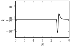
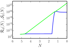
Figure 1: The behavior of the coupling function $\xi$ (on the left) and the corresponding effects on the curvature (in blue) and the isocurvature (in green) perturbations (on the right) have been plotted as a function of e-folds $N$. Recall that time runs forward from left to right and the choice of $N=0$ is arbitrary. There arises a sharp rise in $\xi$ when the direction of evolution changes in the field space. It should be clear from the plots that the amplitude of the curvature perturbation is enhanced exactly around this time.

The analytical expressions for the power spectra we have presented above correspond to spectra evaluated prior to the turn. The power spectra evaluated numerically before and at the turn in field space (when $\phi=\phi_{\rm c}$, corresponding to $\eta=\eta_{\rm c}$) are illustrated in Fig. 2.

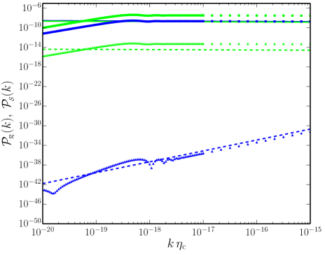
Figure 2: The curvature and isocurvature perturbation spectra, viz. ${\cal P}_{{}_{\!\cal R}}(k)$ and ${\cal P}_{{}_{\!\cal S}}(k)$ (in blue and green, respectively), have been plotted prior to (as dashed lines) as well as during the turn (as solid lines) in field space. Note that ${\cal P}_{{}_{\!\cal S}}(k)$ is nearly scale free both prior to and during the turn. However, while ${\cal P}_{{}_{\!\cal R}}(k)$ is blue before the turn, it is red later. Also, the isocurvature perturbations are extremely dominant prior to the turn. But, the amplitude of the curvature perturbation becomes comparable to that of the isocurvature perturbations during the turn in field space. The range of wavenumbers over which the spectra have been plotted are expected to correspond to cosmological scales today. Moreover, we have chosen to work with values of the various parameters involved so that ${\cal P}_{{}_{\!\cal R}}(k)$ is COBE normalized. The figure also contains the scalar power spectra with a specific feature before (as triangles) and during the turn (as squares). We should highlight that it is the feature in the initial ${\cal P}_{{}_{\!\cal S}}(k)$ which is imprinted as a feature in the final ${\cal P}_{{}_{\!\cal R}}(k)$.

A few points regarding the figure need emphasis. As we discussed, when evaluated prior to the turn, while ${\cal P}_{{}_{\!\cal R}}(k)$ is strongly blue, ${\cal P}_{{}_{\!\cal S}}(k)$ is nearly scale invariant. Also, note that over the scales of interest, the amplitude of ${\cal P}_{{}_{\!\cal S}}(k)$ is considerably larger than the amplitude of ${\cal P}_{{}_{\!\cal R}}(k)$. However, as the turn occurs, we find that both the scalar power spectra have roughly the same amplitude. Moreover, importantly, due to its strong effects, the isocurvature perturbations have altered the shape of the curvature perturbation spectrum ${\cal P}_{{}_{\!\cal R}}(k)$ and, in fact, for suitable values of the parameters, we obtain a nearly scale invariant spectrum with $n_{{}_{\cal R}}\simeq 0.96$, completely consistent with the observations. We have chosen the parameters such that the nearly scale invariant ${\cal P}_{{}_{\!\cal R}}(k)$ is COBE normalized. Below, we shall modify the ekpyrotic potential $V_{\rm ek}(\phi)$ to generate features in the scalar power spectra.

Generating ekpyrotic features: The primordial features that have been found to improve the fit to the data can be broadly classified into the following three types: (1) sharp drop in power at large scales corresponding to the Hubble radius today, (2) a burst of oscillations over an intermediate range of scales, and (3) persisting oscillations over a wide range of scales. While a feature of the first type improves the fit to the CMB data at the very low multipoles (specifically, the low quadrupole) lpq , the second type has been shown to provide a better fit to the outliers (to the nearly scale invariant case) around the multipoles of $\ell\simeq 20$–$40$ flm . The third type of feature has been found to fit the data over a wide range of multipoles oip .

Smooth scalar field potentials cannot generate features. It is the features in the potential and the resulting non-trivial dynamics that translates to features in the power spectra. As we discussed, in inflation, features in the potential lead to deviations from slow roll which, in turn, generate spectra containing departures from near scale invariance. For instance, in single field inflationary models, a point of inflection can lead to the first type of feature we had mentioned above lpq , while the second type of feature can be generated with the introduction of a simple step in the inflationary potential flm . The last type of feature is generated with the aid of corresponding oscillations in the inflationary potential oip . In fact, there have been attempts to construct inflationary models that can simultaneously generate more than one type of features atf .

Since the background dynamics in the ekpyrotic scenario is rather distinct from the inflationary case, prior experience with inflationary features does not necessarily help in constructing ekpyrotic potentials leading to the desired features. We find that multiplying the original ekpyrotic potential $V_{\rm ek}(\phi)$ by the following oscillating term:

$$V_{\rm f}(\phi)=1+\alpha\,{\rm cos}\,(\omega\,\phi/M_{{}_{\rm Pl}})$$ (11)

does indeed lead to persistent oscillations in the power spectrum as in the context of inflation oip . However, the potentials for generating the other two types of features prove to be considerably different. We had to experiment with different multiplicative functions $V_{\rm f}(\phi)$ before arriving at the required forms. Interestingly, we find that, introducing a step by multiplying $V_{\rm ek}(\phi)$ with the term

$$V_{\rm f}(\phi)=1+\alpha\,{\rm tanh}\,[(\phi-\phi_{0})/{\Delta\phi}_{\rm f}]$$ (12)

results in the first type of feature we had mentioned, viz. a sharp drop in power at large scales. Lastly, introducing a well in the potential with the help of a term such as

$$V_{\rm f}(\phi)=1-\alpha\,{\rm exp}\,-\left[(\phi-\phi_{0})/\Delta\phi_{\rm f}\right]^{2}$$ (13)

generates a burst of oscillations over an intermediate range of scales, which is the second type of feature we had discussed. (Though the above modifications to the potentials can be considered to be ad-hoc, we believe that their justification lie in the fact that the CMB data seem to suggest the possibility of features in the primordial spectrum.) We have plotted the power spectra of curvature perturbations arising in these three cases in Fig. 3.

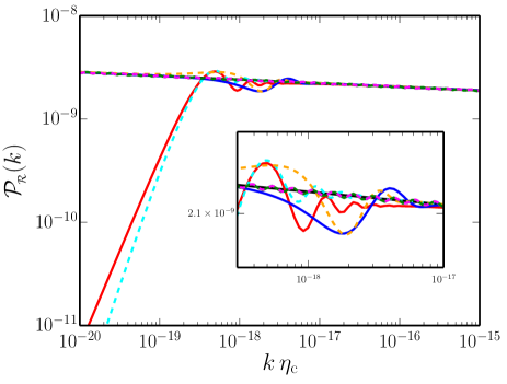
Figure 3: The power spectra of the curvature perturbations with the three types of features (type 1 in red and cyan, type 2 in blue and orange, and type 3 in green and pink) generated in the ekpyrotic (solid lines) and the inflationary (dashed lines) scenarios have been plotted over scales of cosmological interest. The inflationary spectra correspond to those that lead to an improved fit to the CMB data ci . Clearly (as also highlighted in the inset), the ekpyrotic spectra closely resemble the inflationary spectra with features.

In the figure, we have also plotted inflationary power spectra with features that lead to a better fit to the most recent Planck data (in this context, see Refs. planck ). It is clear from the figure that the ekpyrotic features match the inflationary features reasonably well.

Prospects: Features in the primordial spectra can lead to strong constraints on the physics of the early universe fr . However, there is no significant observational evidence for deviations from a nearly scale invariant primordial power spectrum as yet. Many of the simpler and fine tuned bouncing models would prove to be unsustainable if future observations confirm the presence of features planck . We have examined if the bouncing scenarios can remain viable after such a possibility. For the first time, we have constructed ekpyrotic potentials that lead to features that have often been found to provide an improved fit to the CMB data. Though we have evaluated the spectra prior to the bounce, since the scales associated with the bounce are significantly different from the scales of cosmological interest, the shape of the spectra we have arrived at will not be altered by the dynamics of the bounce. Therefore, these power spectra can be expected to retain their form after the bounce (see Refs. fertig-2016 , however, in this context, also see Ref. eob ). Moreover, experience with related models suggests that the isocurvature perturbations would decay after the bounce leading to an adiabatic spectrum consistent with the observations em-rd ; fertig-2016 .

We have focused here on the power spectra generated in the ekpyrotic models. Currently, there also exist strong limits on the primordial scalar non-Gaussianties cpng . The concern has been that, quite generically, the scalar non-Gaussianities generated in bounces may turn out be larger than the current constraints ng-in-em . However, it has been argued that the non-Gaussianities in the type of models we have considered will prove to be small (in this context, see the third reference in Refs. em-rd ). We are currently working towards evaluating the complete scalar bispectrum in bouncing models. We are specifically focusing on the behavior of the bispectrum in the so-called squeezed limit, which may help us discriminate between the inflationary and bouncing scenarios (in this context, see, for instance, Refs. vcr wherein it has been shown that, in contrast to inflation, the consistency relation governing certain three-point functions will be violated in bounces).

Note: As we were finalizing this manuscript, the article fcs appeared on the arXiv which also discusses the generation of features from a contracting phase.

Acknowledgements: The authors wish to thank Debika Chowdhury, Ghanashyam Date, Dhiraj Hazra, Arul Lakshminarayan, James Libby, Jose Mathew and S. Kalyana Rama for comments on the manuscript. LS also wishes to thank the Indian Institute of Technology Madras, Chennai, India, for support through the Exploratory Research Project PHY/17-18/874/RFER/LSRI.

References

- (1) C. L. Bennett et al. Astrophys. J. Suppl. 208, 20 (2013) [arXiv:1212.5225 [astro-ph.CO]].
- (2) P. A. R. Ade et al. [Planck Collaboration], Astron. Astrophys. 571, A15 (2014) [arXiv:1303.5075 [astro-ph.CO]]; N. Aghanim et al. [Planck Collaboration], Astron. Astrophys. 594, A11 (2016) [arXiv:1507.02704 [astro-ph.CO]]; Y. Akrami et al. [Planck Collaboration], arXiv:1807.06205 [astro-ph.CO].
- (3) P. A. R. Ade et al. [Planck Collaboration], Astron. Astrophys. 571, A16 (2014) [arXiv:1303.5076 [astro-ph.CO]]; P. A. R. Ade et al. [Planck Collaboration], Astron. Astrophys. 594, A13 (2016) [arXiv:1502.01589 [astro-ph.CO]]; N. Aghanim et al. [Planck Collaboration], arXiv:1807.06209 [astro-ph.CO].
- (4) P. A. R. Ade et al. [Planck Collaboration], Astron. Astrophys. 571, A22 (2014) [arXiv:1303.5082 [astro-ph.CO]]; P. A. R. Ade et al. [Planck Collaboration], Astron. Astrophys. 594, A20 (2016) [arXiv:1502.02114 [astro-ph.CO]]; Y. Akrami et al. [Planck Collaboration], arXiv:1807.06211 [astro-ph.CO].
- (5) H. Kodama and M. Sasaki, Prog. Theor. Phys. Suppl. 78, 1 (1984); V. F. Mukhanov, H. A. Feldman and R. H. Brandenberger, Phys. Rep. 215, 203 (1992); J. E. Lidsey, A. Liddle, E. W. Kolb, E. J. Copeland, T. Barreiro and M. Abney, Rev. Mod. Phys. 69, 373 (1997) [arXiv:astro-ph/9508078]; A. Riotto, ICTP Lect. Notes Ser. 14, 317 (2003) [arXiv:hep-ph/0210162]; W. H. Kinney, NATO Sci. Ser. II 123, 189 (2003) [astro-ph/0301448]; B. Bassett, S. Tsujikawa and D. Wands, Rev. Mod. Phys. 78, 537 (2006) [arXiv:astro-ph/0507632]; W. H. Kinney, arXiv:0902.1529 [astro-ph.CO]; D. Baumann, arXiv:0907.5424v1 [hep-th]; L. Sriramkumar, Curr. Sci. 97, 868 (2009) [arXiv:0904.4584 [astro-ph.CO]]; L. Sriramkumar in Vignettes in Gravitation and Cosmology, Eds. L. Sriramkumar and T. R. Seshadri (World Scientific, Singapore, 2012), pp. 207–249; J. Martin, Astrophys. Space Sci. Proc. 45, 41 (2016) [arXiv:1502.05733 [astro-ph.CO]]; J. Martin, arXiv:1807.11075 [astro-ph.CO].
- (6) J. Martin, C. Ringeval and V. Vennin, Phys. Dark Univ. 5-6, 75 (2014) [arXiv:1303.3787 [astro-ph.CO]].
- (7) J. Chluba, J. Hamann and S. P. Patil, Int. J. Mod. Phys. D 24, 1530023 (2015) [arXiv:1505.01834 [astro-ph.CO]].
- (8) J. M. Cline, P. Crotty and J. Lesgourgues, JCAP 0309, 010 (2003) [arXiv:astro-ph/0304558]; C. R. Contaldi, M. Peloso, L. Kofman and A. Linde, JCAP 0307, 002 (2003) [arXiv:astro-ph/0303636]; B. A. Powell and W. H. Kinney, Phys. Rev. D 76, 063512 (2007) [arXiv:astro-ph/0612006]; R. K. Jain, P. Chingangbam, J.-O. Gong, L. Sriramkumar and T. Souradeep, JCAP 0901, 009 (2009) [arXiv:0809.3915 [astro-ph]]; R. K. Jain, P. Chingangbam, L. Sriramkumar and T. Souradeep, Phys. Rev. D 82, 023509 (2010) [arXiv:0904.2518 [astro-ph.CO]].
- (9) L. Covi, J. Hamann, A. Melchiorri, A. Slosar and I. Sorbera, Phys. Rev. D 74, 083509 (2006) [arXiv:astro-ph/0606452]; J. Hamann, L. Covi, A. Melchiorri and A. Slosar, Phys. Rev. D 76, 023503 (2007) [arXiv:astro-ph/0701380]; M. J. Mortonson, C. Dvorkin, H. V. Peiris and W. Hu, Phys. Rev. D 79, 103519 (2009) [arXiv:0903.4920 [astro-ph.CO]]; D. K. Hazra, M. Aich, R. K. Jain, L. Sriramkumar and T. Souradeep, JCAP 1010, 008 (2010) [arXiv:1005.2175 [astro-ph.CO]]; M. Benetti, M. Lattanzi, E. Calabrese and A. Melchiorri, Phys. Rev. D 84, 063509 (2011) [arXiv:1107.4992 [astro-ph.CO]]; M. Benetti, Phys. Rev. D 88, 087302 (2013) [arXiv:1308.6406 [astro-ph.CO]].
- (10) M. Aich, D. K. Hazra, L. Sriramkumar and T. Souradeep, Phys. Rev. D 87, 083526 (2013) [arXiv:1106.2798 [astro-ph.CO]]; C. Pahud, M. Kamionkowski and A. R. Liddle, Phys. Rev. D 79, 083503 (2009) [arXiv:0807.0322 [astro-ph]]; P. D. Meerburg, D. N. Spergel and B. D. Wandelt, Phys. Rev. D 89, 063536 (2014) [arXiv:1308.3704 [astro-ph.CO]]; P. D. Meerburg and D. N. Spergel, Phys. Rev. D 89, 063537 (2014) [arXiv:1308.3705 [astro-ph.CO]].
- (11) D. K. Hazra, A. Shafieloo, G. F. Smoot and A. A. Starobinsky, Phys. Rev. Lett. 113, 071301 (2014) [arXiv:1404.0360 [astro-ph.CO]]; D. K. Hazra, A. Shafieloo, G. F. Smoot and A. A. Starobinsky, JCAP 1408, 048 (2014) [arXiv:1405.2012 [astro-ph.CO]];
- (12) D. K. Hazra, A. Shafieloo and T. Souradeep, JCAP 1411, 011 (2014) [arXiv:1406.4827 [astro-ph.CO]]; P. Hunt and S. Sarkar, JCAP 1401, 025 (2014) [arXiv:1308.2317 [astro-ph.CO].
- (13) D. Battefeld and P. Peter, Phys. Rept. 571, 1 (2015) [arXiv:1406.2790 [astro-ph.CO]]; R. Brandenberger and P. Peter, Found. Phys. 47, 797 (2017) [arXiv:1603.05834 [hep-th]].
- (14) L. E. Allen and D. Wands, Phys. Rev. D 70, 063515 (2004) [astro-ph/0404441]; F. Finelli, P. Peter and N. Pinto-Neto, Phys. Rev. D 77, 103508 (2008) [arXiv:0709.3074]; Y.-F. Cai, T. Qiu, R. Brandenberger, Y.-S. Piao and X. Zhang, JCAP 0803 (2008) 013, [arXiv:0711.2187]. Y.-F. Cai, T.-t. Qiu, R. Brandenberger and X.-m. Zhang, Phys. Rev. D 80, 023511, (2009) [arXiv:0810.4677]; Y. F. Cai, D. A. Easson and R. Brandenberger, JCAP 1208, 020 (2012) [arXiv:1206.2382]; R. N. Raveendran, D. Chowdhury, and L. Sriramkumar, JCAP 1801, 030 (2018) [arXiv:1703.10061 [gr-qc]].
- (15) D. A. Easson, I. Sawicki and A. Vikman, JCAP 1111, 021 (2011) [arXiv:1109.1047 [hep-th]]; A. Ijjas and P. J. Steinhardt, Phys. Rev. Lett. 117, 121304 (2016) [arXiv:1606.08880 [gr-qc]]; D. Dobre, A. Frolov, J. Ghersi, S. Ramazanov, A. Vikman JCAP 1803, 020 (2018) [arXiv:1712.10272 [gr-qc]].
- (16) A. M. Levy, Phys. Rev. D 95, 023522 (2017) [arXiv:1611.08972 [gr-qc]].
- (17) J. Khoury, B. A. Ovrut, P. J. Steinhardt and N. Turok, Phys. Rev. D 64, 123522 (2001) [arXiv:hep-th/0103239]; J. L. Lehners, P. McFadden, N. Turok and P. J. Steinhardt, Phys. Rev. D 76, 103501 (2007) [hep-th/0702153 [hep-th]]; E. I. Buchbinder, J. Khoury and B. A. Ovrut, Phys. Rev. D 76, 123503 (2007) [arXiv:hep-th/0702154]; P. Creminelli and L. Senatore, JCAP 0711, 010 (2007) [hep-th/0702165]; K. Koyama and D. Wands, JCAP 0704, 008 (2007) [hep-th/0703040 [hep-th]]; K. Koyama, S. Mizuno and D. Wands, Class. Quant. Grav. 24, 3919 (2007) [arXiv:0704.1152 [hep-th]]; E. I. Buchbinder, J. Khoury and B. A. Ovrut, JHEP 0711, 076 (2007) [arXiv:0706.3903 [hep-th]]; K. Koyama, S. Mizuno, F. Vernizzi and D. Wands, JCAP 0711, 024 (2007) [arXiv:0708.4321 [hep-th]].
- (18) M. Li, Phys. Lett. B 724, 192 (2013) [arXiv:1306.0191 [hep-th]]; T. Qiu, X. Gao and E. N. Saridakis, Phys. Rev. D 88, 043525 (2013) [arXiv:1303.2372 [astro-ph.CO]]; A. Fertig, J.-L. Lehners and E. Mallwitz, Phys. Rev. D 89, 103537 (2014) [arXiv:1310.8133 [hep-th]]; A. Ijjas, J.-L. Lehners and P. J. Steinhardt, Phys. Rev. D 89, 123520 (2014) [arXiv:1404.1265 [astro-ph.CO]]; A. M. Levy, A. Ijjas and P. J. Steinhardt, Phys. Rev. D 92, 063524 (2015) [arXiv:1506.01011 [astro-ph.CO]]; A. Ijjas and P. J. Steinhardt, Class. Quant. Grav. 33, 044001 (2016) [arXiv:1512.09010 [astro-ph.CO]];
- (19) A. Fertig, J.-L. Lehners, E. Mallwitz and E. Wilson-Ewing, JCAP 1610, 005 (2016) [arXiv:1607.05663 [hep-th]].
- (20) J.-L. Lehners, Adv. Astron. 2010, 903907 (2010) [arXiv:1001.3125 [hep-th]].
- (21) Z. Lalak, D. Langlois, S. Pokorski and K. Turzynski, JCAP 0707, 014 (2007) [arXiv:0704.0212 [hep-th]].
- (22) P. Peter, N. Pinto-Neto, and S. D. P. Vitenti, Phys. Rev. D 93, 023520 (2016) [arXiv:1510.06628 [gr-qc]].
- (23) P. A. R. Ade et al. [Planck Collaboration], Astron. Astrophys. 571, A24 (2014) [arXiv:1303.5084 [astro-ph.CO]]; P. A. R. Ade et al. [Planck Collaboration], Astron. Astrophys. 594, A17 (2016) [arXiv:1502.01592 [astro-ph.CO]].
- (24) X. Chen, A. Loeb and Z.-Z. Xianyu, arXiv:1809.02603 [astro-ph.CO].
- (25) J. Martin and P. Peter, Phys. Rev. Lett. 92, 061301 (2004) [astro-ph/0312488].
- (26) D. Chowdhury, V. Sreenath and L. Sriramkumar, JCAP 1511, 002 (2015) [arXiv:1506.06475 [astro-ph.CO]]; D. Chowdhury, L. Sriramkumar and M. Kamionkowski, arXiv:1807.05530v2 [astro-ph.CO].