Convergence analysis of the Magnus-Rosenbrock type method for the finite element discretization of semilinear non-autonomous parabolic PDEs with nonsmooth initial data

Abstract

This paper aims to investigate a full numerical approximation of non-autonomous semilnear parabolic partial differential equations (PDEs) with nonsmooth initial data. Our main interest is on such PDEs where the nonlinear part is stronger than the linear part, also called reactive dominated transport equations. For such equations, many classical numerical methods lose their stability properties. We perform the space and time discretizations respectively by the finite element method and an exponential integrator. We obtain a novel explicit, stable and efficient scheme for such problems called Magnus-Rosenbrock method. We prove the convergence of the fully discrete scheme toward the exact solution. The result shows how the convergence orders in both space and time depend on the regularity of the initial data. In particular, when the initial data belongs to the domain of the family of the linear operator, we achieve convergence orders $\mathcal{O}\left(h^{2}+\Delta t^{2-\epsilon}\right)$, for an arbitrarily small $\epsilon>0$. Numerical simulations to illustrate our theoretical result are provided.

1 Introduction

We consider the following abstract Cauchy problem with boundary conditions

$$u^{\prime}(t)=A(t)u(t)+F(t,u(t)),\quad u(0)=u_{0},\quad t\in(0,T],\quad T>0,$$ (1)

on the Hilbert space $H=L^{2}(\Lambda)$, where $\Lambda$ is an open bounded subset of $\mathbb{R}^{d}$ $(d=1,2,3)$. The family of unbounded linear operators $A(t)$ is assumed to generate an analytic semigroup $S_{s}(t):=e^{A(s)t}$. Suitable assumptions on the nonlinear function $F$ and the linear operator $A(t)$ to ensure the existence of a unique mild solution of (1) are given in the following section. Equation of type (1) finds applications in many fields such as quantum fields theory, electromagnetism, nuclear physics, see e.g. Blanes . Since analytic solutions of (1) are usually not available, numerical algorithms are the only tools to provide good approximations. Numerical schemes for (1) with constant linear operator $A(t)=A$ are widely investigated in the scientific literature, see e.g. Stig1 ; Ostermann5 ; Hochbruck2 ; Ostermann3 and the references therein. If we turn our attention to the non-autonomous case, the list of references becomes remarkably short. In the linear case, (1) has been investigated in Hochbruck1 , where the authors examined the convergence analysis of the Magnus integrator to Schrödinger equation. The Magnus integrator was further investigated in Ostermann1 for PDE (1) with $F$ independent of $u$, where the authors applied the mid-point rule to approximate the Magnus expansion in order to achieve a second order approximation in time. Numercal scheme for semilinear PDEs (1) was investigated in Ostermann4 and the convergence in time has been proved. In Ostermann4 , the authors used the backward Euler method. Although backward Euler method has good stability properties, it is computationally expensive as nonlinear systems need to be solved at each time step. Our goal here is to provide a novel efficient scheme to solve (1) by upgrading the scheme for linear PDEs in Ostermann1 and providing a mathematical rigorous convergence proof in space and in time. A standard direction to upgrade the Magnus integrator Ostermann1 to semilinear PDEs consists to keep the linear structure of (1) at each time step. However, when the linear part of (1) is stronger than its nonlinear part, the PDE (1) is driven by the linear part and the good stability properties of a scheme from such approach it is not guaranteed. Indeed when the nonlinear part of a PDE is stronger than its linear part, the PDE is driven by its nonlinear part. For such problems, keeping the linear structure of (1) at each step yields schemes behaving like the unstable explicit Euler method.

In this paper, we propose a novel numerical scheme by applying the Rosenbrock-Type method Ostermann3 ; finance ; Hochbruck2 ; Hairer ; Antjd2 to the semi-discrete problem (36) combining with the Magnus-integrator to the linearized problem. This combination yields an explicit efficient numerical method for such problems. The linearization technique weakens the nonlinear part such that the linearized semi-discrete problem is driven by its new linear part. In contrast to Ostermann4 , the linearization technique is done at every time step. Note that the Rosenbrock method was investigated in the scientific literature only for autonomous problems, see e.g. Hochbruck2 ; Antjd2 for deterministic problem and recently in Antjd1 for stochastic parabolic PDEs to the best of our knowledge. Moreover, the convergence analyses in Ostermann1 ; Ostermann2 ; Ostermann4 are only in time. Furthermore, we examine the space and time convergence with non smooth initial data where the space discretization is performed using the finite element method. Comparing with scheme in Antjd2 , the analysis here is extremely complicated due to the complexity of $A(t)$ and its semigroup $S_{s}(t)=e^{A(s)t}$. This complexity is broken through novel rigorous mathematical results obtained in Section 3.1. Furthermore, in contrast to the scheme in Antjd2 ; Hochbruck , the new scheme is second order accuracy in time for non-autonomous PDEs (1) with constant linear operator $A$ without the extra matrix exponential function $\varphi_{2}$. Our final convergence result shows how the convergence orders in both space and time depend on the regularity of the initial data. In particular, when the initial data belongs to the domain of the family of the linear operator, we achieve convergence orders $\mathcal{O}\left(h^{2}+\Delta t^{2-\epsilon}\right)$, for an arbitrarily small $\epsilon>0$.

The paper is organized as follows. In Section 2, results about the well posedness are provided along with the Magnus-Rosenbrock scheme (MAGROS) and the main result. The proof of the main result is presented in Section 3. In Section 4, we present some numerical simulations to sustain our theoretical result.

2 Mathematical setting and numerical method

2.1 Notations, settings and well posedness

Let us start by presenting briefly notations, the main function spaces and norms that will be used in this paper. We denote by $\|\cdot\|$ the norm associated to the inner product $\langle\cdot,\cdot\rangle_{H}$ of the Hilbert space $H=L^{2}(\Lambda)$. The norm in the Sobolev space $H^{m}(\Lambda)$, $m\geq 0$ will be denoted by $\|.\|_{m}$. For a Hilbert space $U$ we denote by $\|\cdot\|_{U}$ the norm of $U$, $L(U,H)$ the set of bounded linear operators from $U$ to $H$. For ease of notation, we use $L(U,U)=:L(U)$.

To guarantee the existence of a unique mild solution of (1), and for the purpose of the convergence analysis, we make the following assumptions.

Assumption 2.1

• As in Ostermann1 ; Ostermann2 ; Gonz , we assume that $\mathcal{D}\left(A(t)\right)=D$, $0\leq t\leq T$ and the family of linear operators $A(t):D\subset H\longrightarrow H$ to be uniformly sectorial on $0\leq t\leq T$, i.e. there exist constants $c>0$ and $\theta\in\left(\frac{1}{2}\pi,\pi\right)$ such that

  $$\left\|\left(\lambda\mathbf{I}-A(t)\right)^{-1}\right\|_{L(L^{2}(\Lambda))}\leq\frac{c}{|\lambda|},\quad\lambda\in S_{\theta},$$ (2)

  where $S_{\theta}:=\left\{\lambda\in\mathbb{C}:\lambda=\rho e^{i\phi},\rho>0,0\leq|\phi|\leq\theta\right\}$. As in Ostermann2 , by a standard scaling argument, we assume $-A(t)$ to be invertible with bounded inverse.

• Similarly to Ostermann2 ; Ostermann1 ; Praha ; Gonz , we require the following Lipschitz conditions: there exists a positive constant $K_{1}$ such that

  $$\left\|\left(A(t)-A(s)\right)(-A(0))^{-1}\right\|_{L(H)} \leq K_{1}|t-s|,\quad s,t\in[0,T],$$ (3)

  $$\left\|(-A(0))^{-1}\left(A(t)-A(s)\right)\right\|_{L(D,H)} \leq K_{1}|t-s|,\quad s,t\in[0,T].$$ (4)

• Since we are dealing with non smooth data, we follow Praha and assume that

  $$\mathcal{D}\left(\left(-A(t)\right)^{\alpha}\right)=\mathcal{D}\left(\left(-A(0)\right)^{\alpha}\right),\quad 0\leq t\leq T,\quad 0\leq\alpha\leq 1$$ (5)

  and there exists a positive constant $K_{2}$ such that the following estimate holds uniformly for $t\in[0,T]$

  $$K_{2}^{-1}\left\|\left(-A(0)\right)^{\alpha}u\right\|\leq\left\|(-A(t))^{\alpha}u\right\|\leq K_{2}\left\|(-A(0))^{\alpha}u\right\|,\quad u\in\mathcal{D}\left(\left(-A(0)\right)^{\alpha}\right).$$ (6)

• Similarly to (Ostermann2, , (3.17)) and Gonz ; Ostermann4 , we assume that the map $t\longmapsto A(t)$ is twice differentiable and for any $\alpha_{1},\alpha_{2}\in[0,1]$ such that $\alpha_{1}+\alpha_{2}=1$, the following estimates are satisfied

  $$\|(-A(s))^{-\alpha_{1}}A^{\prime\prime}(t)A(s)^{-\alpha_{2}}\|_{L\left(\left(-A(0)\right)^{1-\alpha_{2}},H\right)} \leq C_{0},\quad s,t\in[0,T],$$

  $$\|(-A(0))^{-\alpha_{1}}(A(t)-A(s))(-A(0))^{-\alpha_{2}}\|_{L\left(\left(-A(0)\right)^{1-\alpha_{2}},H\right)} \leq C_{0}|t-s|,\quad s,t\in[0,T],$$

  where $C_{0}$ is a positive constant independent of $t_{1}$ and $t_{2}$.

Remark 1

From Assumption 2.1 (i) and (iii), it follows that for all $\alpha\geq 0$ and $\delta\in[0,1]$, there exists a constant $C_{1}>0$ such that the following estimates hold uniformly for $t\in[0,T]$

$$\left\|(-A(t))^{\alpha}e^{sA(t)}\right\|_{L(H)}\leq C_{1}s^{-\alpha},\quad\quad s>0,$$ (7)

$$\left\|(-A(t))^{-\delta}\left(\mathbf{I}-e^{sA(t)}\right)\right\|_{L(H)}\leq C_{1}s^{\delta},\quad\quad\quad s\geq 0,$$ (8)

see e.g. (Ostermann2, , (2.1)).

Remark 2

Let $\Delta(T):=\{(t,s):0\leq s\leq t\leq T\}$. It is well known that (Pazy, , Theorem 6.1, Chapter 5) under Assumption 2.1 there exists a unique evolution system (Pazy, , Definition 5.3, Chapter 5) $U:\Delta(T)\longrightarrow L(H)$ such that

• There exists a positive constant $K_{0}$ such that

  $$\|U(t,s)\|_{L(H)}\leq K_{0},\quad 0\leq s\leq t\leq T.$$ (9)

• $U(.,s)\in C^{1}(]s,T];L(H))$, $0\leq s\leq T$,

  $$\frac{\partial U}{\partial t}(t,s)=-A(t)U(t,s),\quad 0\leq s\leq t\leq T,$$ (10)

  $$\|A(t)U(t,s)\|_{L(H)}\leq\frac{K_{0}}{t-s},\quad 0\leq s<t\leq T.$$ (11)

• $U(t,.)v\in C^{1}([0,t[;H)$, $0<t\leq T$, $v\in\mathcal{D}(A(0))$ and

  $$\frac{\partial U}{\partial s}(t,s)v=-U(t,s)A(s)v,\quad 0\leq s\leq t\leq T,$$ (12)

  $$\|A(t)U(t,s)A(s)^{-1}\|_{L(H)}\leq K_{0},\quad 0\leq s\leq t\leq T.$$ (13)

We equip $V_{\alpha}(t):=\mathcal{D}\left(\left(-A(t)\right)^{\alpha/2}\right)$, $\alpha\in\mathbb{R}$ with the norm $\|u\|_{\alpha,t}:=\|(-A(t))^{\alpha/2}u\|$. Due to (5)-(6) and for the seek of ease notations, we simply write $V_{\alpha}$ and $\|.\|_{\alpha}$ instead of $V_{\alpha}(t)$ and $\|.\|_{\alpha,t}$ respectively.

Assumption 2.2

The initial data $u_{0}:\Lambda\longrightarrow H$ is assumed to satisfy $u_{0}\in\mathcal{D}\left(\left(-A(0)\right)^{\beta/2}\right)$, $0\leq\beta\leq 2$.

Similarly to (Lunardi, , (8.1.1)), Ostermann4 and (Stig2, , (5.3)), we make the following assumption on the nonlinear function.

Assumption 2.3

The function $F:[0,T]\times H\longrightarrow H$ is assumed to be twice differentiable with respect to the first and second variables and with bounded partial derivatives, i.e. there exists $K_{3}\geq 0$ such that for $k=\{1,2\}$ we have

$$\left\|\frac{\partial^{2}F}{\partial t\partial u}(t,u)\right\|_{L(H)} \leq K_{3},\quad\left\|\frac{\partial^{k}F}{\partial t^{k}}(t,u)\right\|\leq K_{3}(1+\|u\|),\quad t\in[0,T],\quad u\in H,$$ (14)

$$\left\|\frac{\partial F}{\partial u}(t,u)\right\|_{L(H)} \leq K_{3},\quad\left\|\frac{\partial^{2}F}{\partial u^{2}}(t,u)\right\|_{L(H\times H,H)}\leq K_{3},\quad t\in[0,T],\quad u\in H.$$ (15)

Moreover, we assume assume $F^{\prime}(t,u)$ to be coercive for $t\in[0,T]$ and $u\in H$, i.e. there exists $\kappa>-b_{0}$ such that

$$-\left\langle F^{\prime}(t,u)v,v\right\rangle_{H}\geq\kappa\|v\|^{2},\quad t\in[0,T],\quad v,u\in H,$$ (16)

$$b_{0}=\underset{t\geq 0}{\inf}\{\text{Re}(\lambda(t)),\,\lambda(t)\in\sigma(A(t))\,\,(\text{spectrum of }A(t))\}\,$$ (17)

where $F^{\prime}(t,u):=\frac{\partial F}{\partial u}(t,u)$. We also assume the nonlinear function $F$ to satisfy the Lipschitz condition, i.e. there exists a constant $K_{4}\geq 0$ such that

$$\|F(t,u)-F(s,v)\|\leq K_{4}(|t-s|+\|u-v\|),\quad s,t\in[0,T],\quad u,v\in H.$$ (18)

Indeed from the coercivity (26), we can take $b_{0}=\lambda_{0}$.

The following theorem provides the well posedness of problem (1).

Theorem 2.4

Let Assumption 2.2, Assumption 2.1 and Assumption 2.3 be fulfilled. Then the initial value problem (1) has a unique mild solution $u(t)$ given by

$$u(t)=U(t,0)u_{0}+\int_{0}^{t}U(t,s)F(s,u(s))ds,\quad t\in(0,T],$$ (19)

where $U(t,s)$ is the evolution system defined in Remark  2. Moreover, the following space regularity holds

$$\|(-A(0))^{\beta/2}u(t)\|\leq C\left(1+\|(-A(0))^{\beta/2}u_{0}\|\right),\quad\beta\in[0,2),\quad t\in[0,T].$$ (20)

Proof

Theorem 2.4 is an extension of (Pazy, , Chapter 5, Theorem 7.1) to the full semilinear problem. Its proof can be done using arguments based on a fixed point theorem and the Gronwall’s lemma as of (Pazy, , Chpater 6, Theorem 1.2). The proof of (20) follows from the regularities estimates of the evolution parameter $U(t,s)$.

2.2 Finite element discretization

For the seek of simplicity, we assume the family of linear operators $A(t)$ to be of second order and has the following form

$$A(t)u=\sum_{i,j=1}^{d}\frac{\partial}{\partial x_{i}}\left(q_{ij}(x,t)\frac{\partial u}{\partial x_{j}}\right)-\sum_{j=1}^{d}q_{j}(x,t)\frac{\partial u}{\partial x_{j}}.$$ (21)

We require the coefficients $q_{i,j}$ and $q_{j}$ to be smooth functions of the variable $x\in\overline{\Lambda}$ and Hölder-continuous with respect to $t\in[0,T]$. We further assume that there exists a positive constant $c$ such that the following ellipticity condition holds

$$\sum_{i,j=1}^{d}q_{ij}(x,t)\xi_{i}\xi_{j}\geq c|\xi|^{2},\quad(x,t)\in\overline{\Lambda}\times[0,T].$$ (22)

Under the above assumptions on $q_{ij}$ and $q_{j}$, it is well known that the family of linear operators defined by (21) fulfills Assumption 2.1 (i)-(ii) with $D=H^{2}(\Lambda)\cap H^{1}_{0}(\Lambda)$, see (Pazy, , Section 7.6) or (Tanabe, , Section 5.2). The above assumptions on $q_{ij}$ and $q_{j}$ also imply that Assumption 2.1 (iii) is fulfilled, see e.g. (Praha, , Example 6.1) or Amann ; Seely .

As in Suzuki ; Antonio1 , we introduce two spaces $\mathbb{H}$ and $V$, such that $\mathbb{H}\subset V$, depending on the boundary conditions for the domain of the operator $-A(t)$ and the corresponding bilinear form. For Dirichlet boundary conditions we take

$$V=\mathbb{H}=H^{1}_{0}(\Lambda)=\{v\in H^{1}(\Lambda):v=0\quad\text{on}\quad\partial\Lambda\}.$$ (23)

For Robin boundary condition and Neumann boundary condition, which is a special case of Robin boundary condition ($\alpha_{0}=0$), we take $V=H^{1}(\Lambda)$ and

$$\mathbb{H}=\{v\in H^{2}(\Lambda):\partial v/\partial v_{A}+\alpha_{0}v=0,\quad\text{on}\quad\partial\Lambda\},\quad\alpha_{0}\in\mathbb{R}.$$ (24)

Using Green’s formula and the boundary conditions, we obtain the corresponding bilinear form associated to $-A(t)$

$$a(t)(u,v)=\int_{\Lambda}\left(\sum_{i,j=1}^{d}q_{ij}(x,t)\dfrac{\partial u}{\partial x_{i}}\dfrac{\partial v}{\partial x_{j}}+\sum_{i=1}^{d}q_{i}(x,t)\dfrac{\partial u}{\partial x_{i}}v\right)dx,\quad u,v\in V,$$

for Dirichlet boundary conditions and

$$a(t)(u,v)=\int_{\Lambda}\left(\sum_{i,j=1}^{d}q_{ij}(x,t)\dfrac{\partial u}{\partial x_{i}}\dfrac{\partial v}{\partial x_{j}}+\sum_{i=1}^{d}q_{i}(x,t)\dfrac{\partial u}{\partial x_{i}}v\right)dx+\int_{\partial\Lambda}\alpha_{0}uvdx.$$

for Robin and Neumann boundary conditions. Using Gårding’s inequality, it holds that there exist two constants $\lambda_{0}$ and $c_{0}$ such that

$$a(t)(v,v)\geq\lambda_{0}\|v\|^{2}_{1}-c_{0}\|v\|^{2},\quad v\in V,\quad t\in[0,T].$$ (25)

By adding and subtracting $c_{0}u$ on the right hand side of (1), we obtain a new family of linear operators that we still denote by $A(t)$. Therefore the new corresponding bilinear form associated to $-A(t)$ still denoted by $a(t)$ satisfies the following coercivity property

$$a(t)(v,v)\geq\;\lambda_{0}\|v\|_{1}^{2},\;\;\;\;\;v\in V,\quad t\in[0,T].$$ (26)

Note that the expression of the nonlinear term $F$ has changed as we included the term $-c_{0}u$ in a new nonlinear term that we still denote by $F$.

The coercivity property (26) implies that $A(t)$ is sectorial on $L^{2}(\Lambda)$, see e.g. Stig2 . Therefore $A(t)$ generates an analytic semigroup $S_{t}(s)=e^{sA(t)}$ on $L^{2}(\Lambda)$ such that Henry

$$S_{t}(s)=e^{sA(t)}=\dfrac{1}{2\pi i}\int_{\mathcal{C}}e^{s\lambda}(\lambda I-A(t))^{-1}d\lambda,\;\;\;\;\;\;\;\;s>0,$$ (27)

where $\mathcal{C}$ denotes a path that surrounds the spectrum of $A(t)$. The coercivity property (26) also implies that $-A(t)$ is a positive operator and its fractional powers are well defined and for any $\alpha>0$ we have

$$\left\{\begin{array}[]{rcl}(-A(t))^{-\alpha}&=&\frac{1}{\Gamma(\alpha)}\displaystyle\int_{0}^{\infty}s^{\alpha-1}{\rm e}^{sA(t)}ds,\\ (-A(t))^{\alpha}&=&((-A(t))^{-\alpha})^{-1},\end{array}\right.$$ (28)

where $\Gamma(\alpha)$ is the Gamma function (see Henry ). The domain of $(-A(t))^{\alpha/2}$ are characterized in Suzuki ; Stig1 ; Stig2 for $1\leq\alpha\leq 2$ with equivalence of norms as follows.

$$\mathcal{D}((-A(t))^{\alpha/2}) = H^{1}_{0}(\Lambda)\cap H^{\alpha}(\Lambda)\hskip 28.45274pt\text{(for Dirichlet boundary condition)}$$

$$\mathcal{D}(-A(t)) = \mathbb{H},\quad\mathcal{D}((-A(t))^{1/2})=H^{1}(\Lambda)\hskip 14.22636pt\text{(for Robin boundary condition)}$$

$$\|v\|_{H^{\alpha}(\Lambda)} \equiv \|((-A(t))^{\alpha/2}v\|:=\|v\|_{\alpha},\quad v\in\mathcal{D}((-A(t))^{\alpha/2}).$$

The characterization of $\mathcal{D}((-A(t))^{\alpha/2})$ for $0\leq\alpha<1$ can be found in (Nambu, , Theorem 2.1 & Theorem 2.2).

Let us now move to the space approximation of problem (1). We start with the discretization of our domain $\Lambda$ by a finite triangulation. Let $\mathcal{T}_{h}$ be a triangulation with maximal length $h$. Let $V_{h}\subset V$ denotes the space of continuous and piecewise linear functions over the triangulation $\mathcal{T}_{h}$. As in (Luskin, , (1.6)), we assume that

$$\inf_{\phi_{h}\in V_{h}}\|v-\phi_{h}\|_{j}\leq Ch^{r-j}\|v\|_{r},\quad v\in V\cap H^{r}(\Lambda),\quad r\in\{1,2\},$$ (29)

for all $j\in\{0,1\}$. Moreover, we assume that

$$\inf_{\phi_{h}\in V_{h}}\|v-\phi_{h}\|_{2}\leq C\|v\|_{2},\quad v\in V\cap H^{2}(\Lambda).$$ (30)

We consider the projection $P_{h}$ defined from $H=L^{2}(\Lambda)$ to $V_{h}$ by

$$(P_{h}u,\chi)=(u,\chi),\quad\chi\in V_{h},\,u\in H.$$ (31)

For all $t\in[0,T]$, the discrete operator $A_{h}(t):V_{h}\longrightarrow V_{h}$ is defined by

$$(A_{h}(t)\phi,\chi)=(A(t)\phi,\chi)=-a(t)(\phi,\chi),\quad\phi,\chi\in V_{h}.$$ (32)

The coercivity property (26) implies that there exist two constants $C_{2}>0$ and $\theta\in(\frac{1}{2}\pi,\pi)$ such that (see e.g. (Stig2, , (2.9)) or Suzuki ; Henry )

$$\|(\lambda\mathbf{I}-A_{h}(t))^{-1}\|_{L(H)}\leq\frac{C_{2}}{|\lambda|},\quad\lambda\in S_{\theta}$$ (33)

holds uniformly for $h>0$ and $t\in[0,T]$. The coercivity condition (26) implies that for any $t\in[0,T]$, $A_{h}(t)$ generates an analytic semigroup $S^{h}_{t}(s):=e^{sA_{h}(t)}$, $s\in[0,T]$. The coercivity property (26) also implies that the smooth properties (7) and (8) hold for $A_{h}$ uniformly for $h>0$ and $t\in[0,T]$, i.e. for all $\alpha\geq 0$ and $\delta\in[0,1]$, there exists a positive constant $C_{3}$ such that the following estimates hold uniformly for $h>0$ and $t\in[0,T]$, see e.g. Suzuki ; Henry

$$\left\|(-A_{h}(t))^{\alpha}e^{sA_{h}(t)}\right\|_{L(H)} \leq C_{3}s^{-\alpha},\quad s>0,$$ (34)

$$\left\|(-A_{h}(t))^{-\delta}\left(\mathbf{I}-e^{sA_{h}(t)}\right)\right\|_{L(H)} \leq C_{3}s^{\delta},\quad s\geq 0.$$ (35)

The semi-discrete in space of problem (1) consists of finding $u^{h}(t)\in V_{h}$ such that

$$\dfrac{du^{h}(t)}{dt}=A_{h}(t)u^{h}(t)+P_{h}F(t,u^{h}(t)),\quad u^{h}(0)=P_{h}u_{0},\quad t\in(0,T].$$ (36)

2.3 Fully discrete scheme and main result

Throughout this paper, without loss of generality, we use a fixed time step $\Delta t=T/M$, $M\in\mathbb{N}$ and we set $t_{m}=m\Delta t$, $m\in\mathbb{N}$. The time discretization consists of computing the numerical approximation $u^{h}_{m}$ of $u^{h}(t_{m})$ at discrete times $t_{m}=m\Delta t\in(0,T]$, $\Delta t>0$, $m=0,\cdots,M$. Let us build an explicit scheme, efficient to solve (1). The method is based on the following linearisation of (36) at each time step, aiming to weaken the nonlinear part

$$\dfrac{du^{h}(t)}{dt}=\left[A_{h}(t)+J_{m}^{h}\right]u^{h}(t)+a^{h}_{m}t+G^{h}_{m}(t,u^{h}(t)),\quad t_{m}\leq t\leq t_{m+1},$$ (37)

for $m=0,\cdots,M-1$, where the derivatives $J_{m}^{h}$ and $a^{h}_{m}$ are respectively the partial derivatives of $F$ at $\left(t_{m}+\frac{\Delta t}{2},u^{h}_{m}\right)$ with respect to $u$ and $t$, given by

$$J^{h}_{m}:=P_{h}\frac{\partial F}{\partial u}\left(t_{m}+\frac{\Delta t}{2},u^{h}_{m}\right)\quad\text{and}\quad a^{h}_{m}:=P_{h}\frac{\partial F}{\partial t}\left(t_{m}+\frac{\Delta t}{2},u^{h}_{m}\right)$$ (38)

and the remainder $G^{h}_{m}$ is given by

$$G^{h}_{m}(t,u^{h}(t)):=P_{h}F(t,u^{h}(t))-J_{m}^{h}u^{h}(t)-a^{h}_{m}t.$$ (39)

Note that using Assumption 2.3 the following estimate holds

$$\|J^{h}_{m}u-J^{h}_{m}v\|_{L(H)}\leq K_{3}\|u-v\|,\quad u,v\in H,\quad h>0,\quad m=0,\cdots,M.$$ (40)

It follows therefore from (40), (18) and (39) that the remainder $G^{h}_{m}$ satisfies the following Lipschitz estimate

$$\|G^{h}_{m}(t,u)-G^{h}_{m}(t,v)\|\leq(K_{3}+K_{4})\|u-v\|,\quad u,v\in H,\quad t\in[0,T].$$ (41)

Applying the exponential-like Euler and Midpoint integrators LEM to (37) gives the following numerical scheme, called Magnus-Rosenbrock method (MAGROS)

$$u^{h}_{m+1} = e^{\Delta t\left(A_{h,m}+J^{h}_{m}\right)}u^{h}_{m}+\Delta t\varphi_{1}\left(\Delta t(A_{h,m}+J^{h}_{m})\right)a^{h}_{m}\left(t_{m}+\frac{\Delta t}{2}\right)$$ (42)

$$+ \Delta t\varphi_{1}\left(\Delta t(A_{h,m}+J^{h}_{m})\right)G^{h}_{m}\left(t_{m}+\frac{\Delta t}{2},u^{h}_{m}\right),\quad m=0,\cdots,M-1,$$

where the linear operator $A_{h,m}$ is given by

$$A_{h,m}:=A_{h}\left(t_{m}+\frac{\Delta t}{2}\right)$$ (43)

and the linear function $\varphi_{1}$ is given by

$$\quad\varphi_{1}\left(\Delta t\left(A_{h,m}+J^{h}_{m}\right)\right) := \frac{1}{\Delta t}\int_{0}^{\Delta t}e^{\left(A_{h,m}+J^{h}_{m}\right)(\Delta t-s)}ds.$$ (44)

Note that the numerical scheme (42) can be written in the following form, efficient for simulation

$$u^{h}_{m+1}=u^{h}_{m}+\Delta t\varphi_{1}\left(\Delta t(A_{h,m}+J^{h}_{m})\right)\left[A_{h,m}u^{h}_{m}+P_{h}F\left(t_{m}+\frac{\Delta t}{2},u^{h}_{m}\right)\right].$$ (45)

The numerical scheme (42) can also be written in the following integral form, useful for the error analysis

$$u^{h}_{m+1} = e^{\Delta t\left(A_{h,m}+J^{h}_{m}\right)}u^{h}_{m}+\int_{0}^{\Delta t}e^{\left(A_{h,m}+J^{h}_{m}\right)(\Delta t-s)}a^{h}_{m}\left(t_{m}+\frac{\Delta t}{2}\right)ds$$ (46)

$$+ \int_{0}^{\Delta t}e^{\left(A_{h,m}+J^{h}_{m}\right)(\Delta t-s)}G^{h}_{m}\left(t_{m}+\frac{\Delta t}{2},u^{h}_{m}\right)ds.$$

We will need the following further assumption on the nonlinearity, useful to achieve full convergence order $2$ in space without any logarithmic perturbation when $u_{0}\in\mathcal{D}(-A(0))$. This assumption was also used in (Antonio1, , Remark 2.9).

Assumption 2.5

We assume that $F:[0,T]\times H\longrightarrow H$ satisfies the following estimate

$$\|(-A(s))^{\gamma}F(t,u(r))\|\leq C(\gamma)\left(1+\|(-A(s))^{\gamma}u(r)\|\right),\quad s,r,t\in[0,T],$$ (47)

for any $\gamma>0$ small enough.

We can now state our convergence result, which is in fact the main result of this paper.

Theorem 2.6

[Main result] Let Assumption 2.1, Assumption 2.2 and Assumption 2.3 be fulfilled.

• If $0<\beta<2$, then the following error estimate holds

  $$\|u(t_{m})-u^{h}_{m}\|\leq C\left(h^{\beta}+\Delta t^{1+\beta/2-\epsilon}\right),$$ (48)

  where $\epsilon>0$ is a positive constant small enough.

• If $\beta=2$, then the following error estimate holds

  $$\|u(t_{m})-u^{h}_{m}\|\leq C\left(h^{2}\left(1+\max\left(0,\ln(t_{m}/h)\right)\right)+\Delta t^{2-\epsilon}\right).$$ (49)

• If $\beta=2$ and moreover if Assumption 2.5 is fulfilled then the following error estimate holds

  $$\|u(t_{m})-u^{h}_{m}\|\leq C\left(h^{2}+\Delta t^{2-\epsilon}\right).$$ (50)

Remark 3

Theorem 2.6 extends the result in Ostermann1 to a fully semilinear problem with nonsmooth initial data. Note that the linearisation technique allows to achieve convergence order almost $2$ when $u_{0}\in\mathcal{D}(-A(0))$.

3 Proof of the main result

3.1 Preliminaries results

The following lemma will be useful in our convergence proof.

Lemma 1

Let Assumption 2.1 be fulfilled. Then for any $\gamma\in[0,1]$ the following estimates hold

$$K^{-1}\|(-(A_{h}(0))^{-\gamma}v\| \leq \|((-A_{h}(t))^{-\gamma}v\|\leq K\|((-A_{h}(0))^{-\gamma}v\|,\quad v\in V_{h},$$ (51)

$$K^{-1}\|(-(A_{h}(0))^{\gamma}v\| \leq \|((-A_{h}(t))^{\gamma}v\|\leq K\|((A_{h}(0))^{\gamma}v\|,\quad v\in V_{h},$$ (52)

uniformly in $h>0$ and $t\in[0,T]$, where $K$ is a positive constant independent of $t$ and $h$.

Proof

We only prove (51) since the proof of (52) is similar to (Antjd1, , Lemma 1) by using Assumption 2.1 (iii). For relatively smooth coefficients ($q_{j}\in C^{1}(\Lambda)$), the formal adjoint of $A(t)$ denoted by $A^{*}(t)$ is given by (see e.g. (Evans, , Section 6.2.3))

$$A^{*}(t)=\sum_{i,j=1}^{d}\frac{\partial}{\partial x_{j}}\left(q_{ij}(x,t)\frac{\partial}{\partial x_{i}}\right)+\sum_{j=1}^{d}q_{j}(x,t)\frac{\partial}{\partial x_{j}}+\left(\sum_{j=1}^{d}\frac{\partial q_{j}}{\partial x_{j}}(x,t)\right)\mathbf{I},$$ (53)

for any $t\in[0,T]$. It follows therefore from (53) that $\mathcal{D}(-A^{*}(t))=\mathcal{D}(-A(t))$ for all $t\in[0,T]$. It also follows from (53) that the coefficients of $A^{*}(t)$ satisfy the same assumptions as that of $A(t)$. Therefore from (Praha, , Example 6.1) or Amann ; Seely it holds that $A^{*}(t)$ satisfies Assumption 2.1 (iii). More precisely, for all $\alpha\in[0,1]$ and $t\in[0,1]$, $\mathcal{D}((-A^{*}(t))^{\alpha})=\mathcal{D}((-A^{*}(0))^{\alpha})$ and for all $v\in\mathcal{D}((-A^{*}(0))^{\alpha})$ it holds that

$$C^{-1}\|(-A^{*}(0))^{\alpha}v\|\leq\|(-A^{*}(t))^{\alpha}v\|\leq C\|(-A^{*}(0))^{\alpha}v\|,\quad t\in[0,T].$$ (54)

Note that for all $t\in[0,T]$, $(A^{*}(t))_{h}=A_{h}^{*}(t)$, where $(A^{*}(t))_{h}$ stands for the discrete operator associated to $A^{*}(t)$ and $A_{h}^{*}(t)$ is the adjoint of $A_{h}(t)$. Indeed using (32), it holds that

$$\langle(A^{*}(t))_{h}v,\chi\rangle_{H} = \langle A^{*}(t)v,\chi\rangle_{H}=\langle v,A(t)\chi\rangle_{H}=\langle A(t)\chi,v\rangle_{H}$$ (55)

$$= \langle A_{h}(t)\chi,v\rangle_{H}=\langle\chi,A_{h}^{*}(t)v\rangle_{H}$$

$$= \langle A_{h}^{*}(t)v,\chi\rangle_{H},\quad\chi,v\in V_{h},\quad t\in[0,T],$$

and therefore $(A^{*}(t))_{h}=A_{h}^{*}(t)$ for all $t\in[0,T]$. Let us recall the following equivalence of norms (Stig2, , (2.12)), where we replace $A$ by $A^{*}(t)$

$$\|(-A_{h}^{*}(t))^{1/2}v\|\approx\|(-A^{*}(t))^{1/2}v\|,\quad v\in V_{h},\quad t\in[0,T].$$ (56)

Using (54) and (56) it holds that there exists a positive constant $K$ such that

$$K^{-1}\|(-(A_{h}^{*}(0))^{1/2}v\|\leq\|((-A_{h}^{*}(t))^{1/2}v\|\leq K\|((-A_{h}^{*}(0))^{1/2}v\|,$$ (57)

for any $t\in[0,T]$ and $v\in V_{h}$. Following closely Stig2 or (Stig3, , (3.7)), it holds that

$$\|(-A_{h}(t))^{-1/2}v\| = \sup_{v_{h}\in V_{h}}\frac{|\langle(-A_{h}(t))^{-1/2}v,v_{h}\rangle_{H}|}{\|v_{h}\|}$$ (58)

$$= \sup_{v_{h}\in V_{h}}\frac{|\langle v,(-A_{h}^{*}(t))^{-1/2}v_{h}\rangle_{H}|}{\|v_{h}\|}$$

$$= \sup_{w_{h}\in V_{h}}\frac{|\langle v,w_{h}\rangle_{H}|}{\|(-A_{h}^{*}(t))^{1/2}w_{h}\|},\quad v\in V_{h}.$$

Using (57) yields

$$\sup_{w_{h}\in V_{h}}\frac{|\langle v,w_{h}\rangle_{H}|}{K\|(-A_{h}^{*}(0))^{1/2}w_{h}\|} \leq \sup_{w_{h}\in V_{h}}\frac{|\langle v,w_{h}\rangle_{H}|}{\|(-A_{h}^{*}(t))^{1/2}w_{h}\|}$$ (59)

$$\leq K\sup_{w_{h}\in V_{h}}\frac{|\langle v,w_{h}\rangle_{H}|}{\|(-A_{h}^{*}(0))^{1/2}w_{h}\|}$$

Combining (58) with (59) yields

$$K^{-1}\|(-A_{h}(0))^{-1/2}v\|\leq\|(-A_{h}(t))^{-1/2}v\|\leq\|(-A_{h}(0))^{-1/2}v\|,\quad v\in V_{h}$$ (60)

for all $t\in[0,T]$. Note that (60) obviously holds if we replace $1/2$ by $0$ and by $1$. The proof of the lemma is therefore completed by interpolation theory.

For $t\in[0,T]$, we introduce the Ritz projection $R_{h}(t):V\longrightarrow V_{h}$ defined by

$$\langle-A(t)R_{h}(t)v,\chi\rangle_{H}=\langle-A(t)v,\chi\rangle_{H}=a(t)(v,\chi),\quad v\in V,\quad\chi\in V_{h}.$$ (61)

Under the regularity assumptions on the triangulation (29) and in view of the V-ellipticity condition (22), it is well known (see e.g. (Luskin, , (3.2)) or Ciarlet ; Suzuki ) that the following error estimate holds

$$\|R_{h}(t)v-v\|+h\|R_{h}(t)v-v\|_{H^{1}(\Lambda)}\leq Ch^{r}\|v\|_{H^{r}(\Lambda)},\quad v\in V\cap H^{r}(\Lambda),$$ (62)

for any $r\in[1,2]$. Moreover, using (30) it holds that

$$\|R_{h}(t)v-v\|_{H^{2}(\Lambda)}\leq C\|v\|_{2},\quad v\in V\cap H^{2}(\Lambda),\quad t\in[0,T].$$ (63)

The following error estimate also holds (see e.g. (Luskin, , (3.3)) or Ciarlet ; Suzuki )

$$\|D_{t}\left(R_{h}(t)v-v\right)\|+h\|D_{t}\left(R_{h}(t)v-v\right)\|_{H^{1}(\Lambda)}\leq Ch^{r}\left(\|v\|_{H^{r}(\Lambda)}+\|D_{t}v\|_{H^{r}(\Lambda)}\right),$$ (64)

for any $r\in[1,2]$ and $v\in V\cap H^{r}(\Lambda)$, where $D_{t}:=\frac{\partial}{\partial t}$. The following lemma will be useful in our convergence proof.

Lemma 2

Under Assumption 2.1, the following estimates hold

$$\|(A_{h}(t)-A_{h}(s))(-A_{h}(r))^{-1}u^{h}\| \leq C|t-s|\|u^{h}\|,\quad r,s,t\in[0,T],\quad u^{h}\in V_{h},$$ (65)

$$\|(-A_{h}(r))^{-1}\left(A_{h}(s)-A_{h}(t)\right)u^{h}\| \leq C|s-t|\|u^{h}\|,\quad r,s,t\in[0,T],\quad u^{h}\in V_{h}\cap D.$$ (66)

Moreover for any $u^{h}\in V_{h}\cap\mathcal{D}\left(\left(-A(0)\right)^{1-\alpha_{2}}\right)$ the following estimate holds

$$\|(-A_{h}(0))^{-\alpha_{1}}(A_{h}(t)-A_{h}(s))(-A_{h}(0))^{-\alpha_{2}}u^{h}\| \leq C|t-s|\|u^{h}\|,\quad s,t\in[0,T].$$ (67)

Proof

Using the definition of $A_{h}(t)$ and $A_{h}(s)$ yields

$$\|(A_{h}(t)-A_{h}(s))(-A_{h}(r))^{-1}u^{h}\|^{2}$$ (68)

$$= \left\langle((A_{h}(t)-A_{h}(s))(-A_{h}(r))^{-1}u^{h},((A_{h}(t)-A_{h}(s))(-A_{h}(r))^{-1}u^{h}\right\rangle_{H}$$

$$= \left\langle((A(t)-A(s))(-A_{h}(r))^{-1}u^{h},((A_{h}(t)-A_{h}(s))(-A_{h}(r))^{-1}u^{h}\right\rangle_{H}.$$

Using Cauchy’s Schwartz inequality, the relation $A_{h}(r)R_{h}(r)=P_{h}A(r)$ (see e.g. Antonio1 ; Stig2 ), Assumption 2.1 (ii) and the boundness of $R_{h}(r)$ yields

$$\|(A_{h}(t)-A_{h}(s))(-A_{h}(r))^{-1}u^{h}\|$$ (69)

$$\leq C\|((A(t)-A(s))(-A_{h}(r))^{-1}u^{h}\|$$

$$= C\|((A(t)-A(s))(-A_{h}(r))^{-1}P_{h}u^{h}\|$$

$$= C\|((A(t)-A(s))R_{h}(r)(-A(r))^{-1}u^{h}\|$$

$$= C\|((A(t)-A(s))(-A(r))^{-1}(-A(r))R_{h}(r)(-A(r))^{-1}u^{h}\|$$

$$\leq C|t-s|\|(-A(r))R_{h}(r)(-A(r))^{-1}u^{h}\|.$$

Using triangle inequality and (63) yields

$$\|(-A(r))R_{h}(r)(-A(r))^{-1}u^{h}\|$$ (70)

$$\leq \|(-A(r))R_{h}(r)(-A(r))^{-1}u^{h}-A(r)(-A(r))^{-1}u^{h}\|+\|A(r)(-A(r))^{-1}u^{h}\|$$

$$= \left\|A(r)\left(R_{h}(r)(-A(r))^{-1}u^{h}-(-A(r))^{-1}u^{h}\right)\right\|+\|u^{h}\|$$

$$= \|R_{h}(r)(-A(r))^{-1}u^{h}-(-A(r))^{-1}u^{h}\|_{H^{2}(\Lambda)}+\|u^{h}\|$$

$$\leq C\|(-A(r))^{-1}u^{h}\|_{H^{2}(\Lambda)}+\|u^{h}\|$$

$$\leq C\|u^{h}\|.$$

Substituting (70) in (69) yields

$$\|(A_{h}(t)-A_{h}(s))(-A_{h}(r))^{-1}u^{h}\|\leq C|t-s|\|u^{h}\|.$$ (71)

This completes the proof of (65).

To prove (66), as in Antonio2 or Stig2 we set $V_{r}=\mathcal{D}(-A(r))$, $V_{r}^{h}=\mathcal{D}(-A_{h}(r))$, so $V^{\prime}_{r}=\mathcal{D}\left((-A(r))^{-1}\right)$. Following (Antonio2, , (67)) or Stig2 , we have

$$\left\|(-A_{h}(r))^{-1}\left(A_{h}(s)-A_{h}(t)\right)u^{h}\right\|=\sup_{v_{h}\in V_{r}^{h}}\frac{\left\langle\left(A_{h}(s)-A_{h}(t)\right)u^{h},(-A^{*}_{h}(r))^{-1}v_{h}\right\rangle_{H}}{\|v_{h}\|}$$

Using the definition of $A_{h}(s)$ and $A_{h}(t)$, it holds that

$$\left\|(-A_{h}(r))^{-1}\left(A_{h}(s)-A_{h}(t)\right)u^{h}\right\| = \sup_{v_{h}\in V_{r}^{h}}\frac{\left\langle\left(A(s)-A(t)\right)u^{h},(-A^{*}_{h}(r))^{-1}v_{h}\right\rangle_{H}}{\|v_{h}\|}$$ (72)

$$= \sup_{w_{h}\in V_{r}^{h}}\frac{\left\langle\left(A(s)-A(t)\right)u^{h},w_{h}\right\rangle_{H}}{\|(-A^{*}_{h}(r))w_{h}\|}$$

$$\leq C\sup_{w_{h}\in V_{r}^{h}}\frac{\left\langle\left(A(s)-A(t)\right)u^{h},w_{h}\right\rangle_{H}}{\|w_{h}\|_{V_{r}}}$$

$$= C\left\|\left(A(s)-A(t)\right)u^{h}\right\|_{-1}$$

$$= C\left\|(-A(r))^{-1})\left(A(s)-A(t)\right)u^{h}\right\|$$

$$\leq C|s-t|\,\|u^{h}\|,$$

where Assumption 2.1 (ii) is used at the last step. This completes the proof of (66). The proof of (67) follows from (66) and (65) by interpolation theory.

Lemma 3

Let Assumption 2.1 be fulfilled. Then for any $u^{h}\in V_{h}\cap\mathcal{D}\left(\left(-A(0)\right)^{1-\alpha_{2}}\right)$ the following estimates hold

$$\|(-A_{h}(0))^{-\alpha_{1}}A_{h}^{\prime}(t)(-A_{h}(0))^{-\alpha_{2}}u^{h}\| \leq C\|u^{h}\|,\quad t\in[0,T],$$ (73)

$$\|(-A_{h}(0))^{-\alpha_{1}}A_{h}^{\prime\prime}(t)(-A_{h}(0))^{-\alpha_{2}}u^{h}\| \leq C\|u^{h}\|,\quad t\in[0,T],$$ (74)

where $\alpha_{1}$ and $\alpha_{2}$ are defined in Assumption 2.1.

Proof

Recall that

$$A_{h}^{\prime}(t)=\lim_{\delta\longrightarrow 0}\frac{A_{h}(t+\delta)-A_{h}(t)}{\delta}.$$ (75)

The proof of (73) is completed by combining (67) and (75). The proof of (74) follows the same lines as that of Lemma 2.

Remark 4

From Lemma 2, it follows (Pazy, , Theorem 6.1, Chapter 5) that there exists a unique evolution system $U_{h}:\Delta(T)\longrightarrow L(H)$, satisfying (Pazy, , (6.3), Page 149)

$$U_{h}(t,s)=S^{h}_{s}(t-s)+\int_{s}^{t}S^{h}_{\tau}(t-\tau)R^{h}(\tau,s)d\tau,$$ (76)

where $S^{h}_{s}(t):=e^{A_{h}(s)t}$, $R^{h}(t,s):=\sum\limits_{m=1}^{\infty}R^{h}_{m}(t,s)$, with $R^{h}_{m}(t,s)$ satisfying the following recurrence relation (Pazy, , (6.22), Page 153)

$$R^{h}_{m+1} = \int_{s}^{t}R^{h}_{1}(t,s)R^{h}_{m}(\tau,s)d\tau,$$ (77)

$$R^{h}_{1}(t,s) := (A_{h}(s)-A_{h}(t))S^{h}_{s}(t-s),\quad m\geq 1$$ (78)

Note also that from (Pazy, , (6.6), Chpater 5, Page 150), the following identity holds

$$R^{h}(t,s)=R_{1}^{h}(t,s)+\int_{s}^{t}R_{1}^{h}(t,\tau)R^{h}(\tau,s)d\tau.$$ (79)

The mild solution of (36) is therefore given by

$$u^{h}(t)=U_{h}(t,0)P_{h}u_{0}+\int_{0}^{t}U_{h}(t,s)P_{h}F(s,u^{h}(s))ds.$$ (80)

Lemma 4

Under Assumption 2.1, the evolution system $U_{h}:\Delta(T)\longrightarrow H$ satisfies the following properties

• $U_{h}(.,s)\in C^{1}(]s,T];L(H))$, $0\leq s\leq T$ and

  $$\frac{\partial U_{h}}{\partial t}(t,s)=-A_{h}(t)U_{h}(t,s),\quad 0\leq s\leq t\leq T,$$ (81)

  $$\|A_{h}(t)U_{h}(t,s)\|_{L(H)}\leq\frac{C}{t-s},\quad 0\leq s<t\leq T.$$ (82)

• $U_{h}(t,.)u\in C^{1}([0,t[;H)$, $0<t\leq T$, $u\in\mathcal{D}(A_{h}(0))$ and

  $$\frac{\partial U_{h}}{\partial s}(t,s)u=-U_{h}(t,s)A_{h}(s)u,\quad 0\leq s\leq t\leq T$$ (83)

  $$\|A_{h}(t)U_{h}(t,s)A_{h}(s)^{-1}\|_{L(H)}\leq C,\quad 0\leq s\leq t\leq T.$$ (84)

Proof

The proof is similar to that of (Pazy, , Theorem 6.1, Chapter 5) by using (35), (34), Lemma 2 and Lemma 1.

Lemma 5

Let Assumption 2.1 be fulfilled.

• The following estimates hold

  $$\|R^{h}_{1}(t,s)\|_{L(H)}\leq C, \quad\|R^{h}_{m}(t,s)\|_{L(H)}\leq\frac{C}{m!}(t-s)^{m-1},\quad m\geq 1,$$ (85)

  $$\|R^{h}(t,s)\|_{L(H)}\leq C, \quad\|U_{h}(t,s)\|_{L(H)}\leq C,\quad 0\leq s\leq t\leq T.$$ (86)

• For any $0\leq\gamma\leq\alpha\leq 1$ and $0\leq s\leq t\leq T$, the following estimates hold

  $$\|(-A_{h}(r))^{\alpha}U_{h}(t,s)\|_{L(H)} \leq C(t-s)^{-\alpha},\quad r\in[0,T],$$ (87)

  $$\|U_{h}(t,s)(-A_{h}(r))^{\alpha}\|_{L(H)} \leq C(t-s)^{-\alpha},\quad r\in[0,T],$$ (88)

  $$\|(-A_{h}(r))^{\alpha}U_{h}(t,s)(-A_{h}(s))^{-\gamma}\|_{L(H)} \leq C(t-s)^{\gamma-\alpha},\quad r\in[0,T].$$ (89)

• For any $0\leq s\leq t\leq T$ the following useful estimates hold

  $$\|\left(U_{h}(t,s)-\mathbf{I}\right)(-A_{h}(s))^{-\gamma}\|_{L(H)} \leq C(t-s)^{\gamma},\quad 0\leq\gamma\leq 1,$$ (90)

  $$\|\left(-A_{h}(r))^{-\gamma}(U_{h}(t,s)-\mathbf{I}\right)\|_{L(H)} \leq C(t-s)^{\gamma},\quad 0\leq\gamma\leq 1.$$ (91)

Proof

• The proof of the first estimate of (201) follows the same lines as (Pazy, , Corollary 6.3, Page 153) by using (34), Lemmas 1 and 2. The proof of the second estimate of (201) follows the same lines as (Pazy, , (6.23), Page 153). The proof of the first estimate of (86) is similar to (Pazy, , (6.26), Page 153) and the proof of the second estimate of (86) is similar to (Pazy, , (6.27), Page 153).

• The estimate of (87) for $\alpha=1$ is given in Lemma 4. The proof of (87) for the case $0\leq\alpha<1$ follows from the integral equation (76). In fact pre-multiplying both sides of (76) by $(-A_{h}(s))^{\alpha}$, taking the norm in both sides, using Lemma 1 and (34) yields

  $$\|(-A_{h}(r))^{\alpha}U_{h}(t,s)\|_{L(H)} \leq \|(-A_{h}(r))^{\alpha}S_{s}^{h}(t-s)\|_{L(H)}$$ (92)

  $$+ \int_{s}^{t}\|(-A_{h}(r))^{\alpha}S_{\tau}^{h}(t-\tau)\|_{L(H)}\|R^{h}(\tau,s)\|_{L(H)}d\tau$$

  $$\leq C(t-s)^{-\alpha}+C\int_{s}^{t}(t-\tau)^{-\alpha}d\tau$$

  $$\leq C(t-s)^{-\alpha}.$$

  This proves (87). The proof of (89) and (88) are similar to that of (87).

• From (76), it holds that

  $$(U_{h}(t,s)-\mathbf{I})(-A_{h}(r))^{-\gamma} = (-A_{h}(s))^{-\gamma}\left(e^{A(s)(t-s)}-\mathbf{I}\right)$$ (93)

  $$+ \int_{s}^{t}S^{h}_{\tau}(t-\tau)R^{h}(\tau,s)(-A_{h}(s))^{-\gamma}d\tau.$$

  Taking the norm in both sides of (93), using (35), the boundness of $(-A_{h}(r))^{-\gamma}$ and Lemma 5 (i) yields

  $$\|(U_{h}(t,s)-\mathbf{I})(-A_{h}(s))^{-\gamma}\|_{L(H)} = C(t-s)^{\gamma}+C\int_{s}^{t}d\tau\leq C(t-s)^{\gamma}.$$

  This completes the proof of (90). The proof of (91) is similar to that of (90).

The following space regularity of the semi-discrete problem (36) will be useful in our convergence analysis.

Lemma 6

Let Assumption 2.1 (i)-(ii), Assumption 2.2 and Assumption 2.3 be fulfilled with the corresponding $0\leq\beta<2$. Then for all $\gamma\in[0,\beta]$ and $\alpha\in[0,2)$ the following estimates hold

$$\|(-A_{h}(r))^{\gamma/2}u^{h}(t)\| \leq C,\quad\hskip 56.9055pt0\leq r,t\leq T,$$ (94)

$$\|(-A_{h}(0))^{\alpha/2}u^{h}(t)\| \leq Ct^{\beta/2-\alpha/2},\quad t\in[0,T],\quad\beta\in[0,2],$$ (95)

Proof

We first show that

$$\|u^{h}(t)\|\leq C,\quad t\in[0,T].$$ (96)

Taking the norm in both side of (80) and using the triangle inequality yields

$$\|u^{h}(t)\|\leq\|U_{h}(t,0)P_{h}u_{0}\|+\left\|\int_{0}^{t}U_{h}(t,s)P_{h}F(s,u^{h}(s))ds\right\|ds:=I_{0}+I_{1}.$$ (97)

Using Lemma 5 (i) and the uniformly boundedness of $P_{h}$, it holds that

$$I_{0}\leq\|u_{0}\|\leq C.$$ (98)

Using Lemma 5 (i), Assumption 2.3 and the uniformly boundedness of $P_{h}$, it holds that

$$I_{1} \leq \int_{0}^{t}\|U_{h}(t,s)P_{h}F(s,u^{h}(s))\|\leq C\int_{0}^{t}\left(C+\|u^{h}(s)\|\right)ds$$ (99)

$$\leq C+C\int_{0}^{t}\|u^{h}(s)\|ds.$$

Substituting (99) and (98) in (97) yields

$$\|u^{h}(t)\|\leq C+C\int_{0}^{t}\|u^{h}(s)\|ds.$$ (100)

Applying the continuous Gronwall’s lemma to (100) completes the proof of (96). Let us now prove (94). Pre-multiplying (80) by $(-A_{h}(r))^{\gamma/2}$, taking the norm in both sides and using triangle inequality yields

$$\left\|(-A_{h}(r))^{\gamma/2}u^{h}(t)\right\| \leq \left\|(-A_{h}(r))^{\gamma/2}U_{h}(t,0)P_{h}u_{0}\right\|_{L(H)}$$ (101)

$$+ \int_{0}^{t}\left\|(-A_{h}(r))^{\gamma/2}U_{h}(t,s)P_{h}F(s,u^{h}(s))\right\|ds$$

$$=: II_{0}+II_{1}.$$

Inserting $(-A_{h}(0))^{-\gamma/2}(-A_{h}(0))^{\gamma/2}$, using Lemma 5 (ii) and Lemma 1, it holds that

$$II_{0}\leq\|(-A_{h}(r))^{\gamma/2}U_{h}(t,0)(-A_{h}(0))^{-\gamma/2}\|_{L(H)}\|(-A_{h}(0))^{\gamma/2}u_{0}\|\leq C.$$ (102)

Using Lemma 1, Lemma 5 (ii), Assumption 2.3 and (96) yields

$$II_{1} \leq C\left(\int_{0}^{t}\left\|(-A_{h}(s))^{\gamma/2}U_{h}(t,s)\right\|_{L(H)}ds\right)\sup_{r\in[0,T]}\left\|F\left(r,u^{h}(r)\right)\right\|$$ (103)

$$\leq C\sup_{s\in[0,T]}\left(1+\|u^{h}(s)\|\right)\int_{0}^{t}(t-s)^{-\gamma/2}ds\leq C.$$

Substituting (103) and (102) in (101) completes the proof of (94). The proof of (95) is similar to that of (94). This completes the proof of Lemma 6.

Let us consider the following deterministic problem: find $w\in V$ such that

$$w^{\prime}=A(t)w,\quad w(\tau)=v,\quad t\in(\tau,T].$$ (104)

The corresponding semi-discrete problem in space is: find $w_{h}\in V_{h}$ such that

$$w_{h}^{\prime}(t)=A_{h}(t)w_{h},\quad w_{h}(\tau)=P_{h}v,\quad t\in(\tau,T],\quad\tau\geq 0.$$ (105)

Let us define the operator

$$T_{h}(t,\tau):=U(t,\tau)-U_{h}(t,\tau)P_{h},$$ (106)

so that $w(t)-w_{h}(t)=T_{h}(t,\tau)v$. The following lemma will be useful in our convergence analysis.

Lemma 7

Let $r\in[0,2]$ and $\gamma\leq r$. Let Assumption 2.1 be fulfilled. Then the following error estimate holds for the semi-discrete approximation (105)

$$\|w(t)-w_{h}(t)\|=\|T_{h}(t,\tau)v\|\leq Ch^{r}(t-\tau)^{-(r-\gamma)/2}\|v\|_{\gamma},$$ (107)

for any $v\in\mathcal{D}\left(\left(-A(0)\right)^{\gamma/2}\right)$.

Proof

As in (Antonio1, , (3.5)) or Stig2 , we set

$$w_{h}(t)-w(t) = \left(w_{h}(t)-R_{h}(t)w(t)\right)+\left(R_{h}(t)w(t)-w(t)\right)$$ (108)

$$\equiv \theta(t)+\rho(t).$$

Using the definition of $R_{h}(t)$ and $P_{h}$, we can prove exactly as in Stig2 ; Antonio1 that

$$A_{h}(t)R_{h}(t)=P_{h}A(t),\quad t\in[0,T].$$ (109)

One can easily compute the following derivatives

$$\theta_{t} = A_{h}(t)w_{h}(t)-R_{h}^{\prime}(t)w(t)-R_{h}(t)A(t)w(t),$$ (110)

$$D_{t}\rho = R_{h}^{\prime}(t)w(t)+R_{h}(t)A(t)w(t)-A(t)w(t).$$ (111)

Endowing $V$ and the linear subspace $V_{h}$ with the $\|.\|_{H^{1}(\Lambda)}$ norm, it follows from (62) that $R_{h}(t)\in L(V,V_{h})$ for all $t\in[0,T]$. By the definition of the differential operator, it follows that $R_{h}^{\prime}(t)\in L(V,V_{h})$ for all $t\in[0,T]$. Hence $P_{h}R_{h}^{\prime}(t)=R_{h}^{\prime}(t)$ for all $t\in[0,T]$ and it follows from (111) that

$$P_{h}D_{t}\rho=R_{h}^{\prime}(t)w(t)+R_{h}(t)A(t)w(t)-P_{h}A(t)w(t).$$ (112)

Adding and subtracting $P_{h}A(t)w(t)$ in (110) and using (109), it follows that $\theta$ satisfies the following equation

$$\theta_{t}=A_{h}(t)\theta-P_{h}D_{t}\rho,\quad t\in(\tau,T],$$ (113)

Since $\{A_{h}(t)\}_{t\in[0,T]}$ generates an evolution system $\{U_{h}(t,s)\}_{0\leq s\leq t\leq T}$, it holds that

$$\theta(t)=U_{h}(t,\tau)\theta(\tau)-\int_{\tau}^{t}U_{h}(t,s)P_{h}D_{s}\rho(s)ds.$$ (114)

Splitting the integral part of (114) into two intervals and integrating by parts over the first interval yields

$$\theta(t) = U_{h}(t,\tau)\theta(\tau)+U_{h}(t,\tau)P_{h}\rho(\tau)-U_{h}\left(t,(t+\tau)/2\right)P_{h}\rho\left((t+\tau)/2\right)$$ (115)

$$+ \int_{\tau}^{(t+\tau)/2}\frac{\partial}{\partial s}\left(U_{h}(t,s)\right)P_{h}\rho(s)ds-\int_{(t+\tau)/2}^{t}U_{h}(t,s)P_{h}D_{s}\rho(s)ds.$$

Using the expression of $\theta(\tau)$, $\rho(\tau)$ and the fact that $u_{h}(\tau)=P_{h}v$, it holds that

$$\theta(\tau)+P_{h}\rho(\tau)=0.$$ (116)

Using (116) reduces (115) to

$$\theta(t) = -U_{h}(t,s)P_{h}\rho((t+\tau)/2)+\int_{\tau}^{(t+\tau)/2}\frac{\partial}{\partial s}\left(U_{h}(t,s)\right)P_{h}\rho(s)ds$$ (117)

$$- \int_{(t+\tau)/2}^{t}U_{h}(t,s)P_{h}D_{s}\rho(s)ds.$$

Taking the norm in both sides of (117), using the uniformly boundedness of $P_{h}$, (34), Lemma 2 and Lemma 5 (i) yields

$$\|\theta(t)\| \leq C\|\rho((t+\tau)/2)\|+\int_{\tau}^{(t+\tau)/2}\left\|U_{h}(t,s)A_{h}(s)\right\|_{L(H)}\|\rho(s)\|ds+\int_{(t+\tau)/2}^{t}\|D_{s}\rho(s)\|ds$$ (118)

$$\leq C\|\rho((t+\tau)/2)\|+\int_{\tau}^{(t+\tau)/2}(t-s)^{-1}\|\rho(s)\|ds+\int_{(t+\tau)/2}^{t}\|D_{s}\rho(s)\|ds.$$

Using (62), it holds that

$$\|\rho(s)\|\leq Ch^{r}\|w(s)\|_{r}.$$ (119)

Note that the solution of (104) is represented as follows.

$$w(s)=U(s,\tau)v,\quad s\geq\tau.$$ (120)

Pre-multiplying both sides of (120) by $(-A(s))^{r/2}$, inserting an appropriate power of $-A(\tau)$, using Lemma 5 (ii) and (Antjd1, , Lemma 1) yields

$$\|(-A(t))^{r/2}w(s)\| \leq \|(-A(s))^{r/2}U(s,\tau)(-A(\tau))^{-\gamma/2}\|_{L(H)}\|(-A(\tau))^{\gamma/2}v\|$$ (121)

$$\leq C(s-\tau)^{-(r-\gamma)/2}\|(-A(\tau))^{\gamma/2}v\|$$

$$\leq C(s-\tau)^{-(r-\gamma)/2}\|v\|_{\gamma}.$$

Therefore it holds that

$$\|w(s)\|_{r}\leq C(s-\tau)^{-(r-\gamma)/2}\|v\|_{\gamma},\quad 0\leq\gamma\leq r\leq 2,\quad\tau<s.$$ (122)

Substituting (122) in (119) yields

$$\|\rho(s)\|_{r}\leq Ch^{r}(s-\tau)^{-(r-\gamma)/2}\|v\|_{\gamma}.$$ (123)

Using (64), it holds that

$$\|D_{s}\rho(s)\|\leq Ch^{r}(\|w(s)\|_{r}+\|D_{s}w(s)\|_{r}).$$ (124)

Taking the derivative with respect to $s$ in both sides of (120) yields

$$D_{s}w(s)=A(s)U(s,\tau)v.$$ (125)

As for (121), pre-multiplying both sides of (125) by $(-A(s))^{r/2}$, inserting $(-A(\tau))^{-\gamma/2}(-A(\tau))^{\gamma/2}$ and using Lemma 5 (ii) yields

$$\|D_{s}w(s)\|_{r}\leq C(s-\tau)^{-1-(r-\gamma)/2}\|v\|_{\gamma}.$$ (126)

Substituting (122) and (126) in (124) yields

$$\|D_{s}\rho(s)\| \leq Ch^{r}\left((s-\tau)^{-(r-\gamma)/2}\|v\|_{\gamma}+(s-\tau)^{-1-(r-\gamma)/2}\|v\|_{\gamma}\right)$$ (127)

$$\leq Ch^{r}(s-\tau)^{-1-(r-\gamma)/2}\|v\|_{\gamma}.$$

Substituting (123) and (127) in (118) yields

$$\|\theta(t)\| \leq Ch^{r}(t-\tau)^{-(r-\gamma)/2}\|v\|_{\gamma}$$ (128)

$$+ Ch^{r}\int_{\tau}^{(t+\tau)/2}(t-s)^{-1}(s-\tau)^{-(r-\gamma)/2}\|v\|_{\gamma}ds$$

$$+ Ch^{r}\int_{(t+\tau)/2}^{t}(s-\tau)^{-1-(r-\gamma)/2}\|v\|_{\gamma}ds.$$

Using the estimate

$$\int_{\tau}^{(t+\tau)/2}(t-s)^{-1}(s-\tau)^{-(r-\gamma)/2}ds+\int_{(t+\tau)/2}^{t}(s-\tau)^{-1-(r-\gamma)/2}ds\leq C(t-\tau)^{-(r-\gamma)/2},$$

it follows that

$$\|\theta(t)\|\leq Ch^{r}(t-\tau)^{-(r-\gamma)/2}\|v\|_{\gamma}.$$ (129)

Substituting (129) and (124) in (108) yields

$$\|w(t)-w_{h}(t)\|\leq\|\theta(t)\|+\|\rho(t)\|\leq Ch^{r}(t-\tau)^{-(r-\gamma)/2}\|v\|_{\gamma}.$$ (130)

This completes the proof of Lemma 7.

Remark 5

Lemma 7 generalizes (Antonio1, , Lemma 3.1) to time dependent problems. It also generalises (Luskin, , Lemmas 3.2 and 3.3) and (Thomee1, , Theorems 3 and 4) to more general boundary conditions than only Dirichlet boundary conditions. Note that the fact that the solution vanishes at the boundary is fundamental in the proof of (Luskin, , Lemmas 3.2 and 3.3) and (Thomee1, , Theorems 3 and 4), where authors used energy estimates arguments.

The following theorem gives the space convergence error of the semi-discrete solution in space toward the exact solution. It is fundamental in the proof of the convergence of the fully discrete scheme.

Theorem 3.1

Let Assumption 2.1, Assumption 2.2 and Assumption 2.3 be fulfilled. Let $u(t)$ and $u^{h}(t)$ be the mild solution of (1) and (36) respectively.

• If $0<\beta<2$, then the following error estimate holds

  $$\|u(t)-u^{h}(t)\|\leq Ch^{\beta},\quad 0\leq t\leq T.$$ (131)

• If $\beta=2$, then the following error estimate holds

  $$\|u(t)-u^{h}(t)\|\leq Ch^{2}\left(1+\max\left(0,\ln(t/h^{2})\right)\right),\quad 0<t\leq T.$$ (132)

• If $\beta=2$ and if further Assumption 2.5 is fulfilled, then the following error estimate holds

  $$\|u(t)-u^{h}(t)\|\leq Ch^{2},\quad 0\leq t\leq T.$$ (133)

Proof

Subtracting (80) form (19), taking the norm and using triangle inequality yields

$$\|u(t)-u^{h}(t)\| \leq \left\|U(t,0)u_{0}-U_{h}(t,0)P_{h}u_{0}\right\|$$ (134)

$$+ \left\|\int_{0}^{t}\left[U(t,s)F\left(s,u(s)\right)-U_{h}(t,s)P_{h}F\left(s,u^{h}(s)\right)\right]ds\right\|$$

$$=: III_{0}+III_{1}.$$

Using Lemma 7 with $r=\gamma=\beta$ yields

$$III_{0}\leq Ch^{\beta}\|u_{0}\|\leq Ch^{\beta}.$$ (135)

Using Lemma 7 with $r=\beta$ (with $\beta<2$), $\gamma=0$, Assumption 2.3, Lemma 6 and Lemma 5 yields

$$III_{1} \leq \int_{0}^{t}\left\|U(t,s)F\left(s,u(s)\right)-U(t,s)F\left(s,u^{h}(s)\right)\right\|ds$$ (136)

$$+ \int_{0}^{t}\left\|U(t,s)F\left(s,u^{h}(s)\right)-U_{h}(t,s)P_{h}F\left(s,u^{h}(s)\right)\right\|ds$$

$$\leq C\int_{0}^{t}\left\|u(s)-u^{h}(s)\right\|_{L^{2}(\Omega,H)}ds+Ch^{\beta}\int_{0}^{t}(t-s)^{-\beta/2}ds$$

$$\leq Ch^{\beta}+C\int_{0}^{t}\left\|u(s)-u^{h}(s)\right\|ds.$$

Substituting (136) and (135) in (134) yields

$$\left\|u(t)-u^{h}(t)\right\|\leq Ch^{\beta}+C\int_{0}^{t}\left\|u(s)-u^{h}(s)\right\|ds.$$ (137)

Applying the continuous Gronwall’s lemma to (137) prove (131). The proof of (132) is straightforward. This completes the proof of Proposition 3.1.

The following lemma extends some results in Luskin (see e.g. (Luskin, , Lemma 2.4, (2.8)) and (Luskin, , Lemma 2.6)) to the case of fully semilinear problem. It also extends (Antjd2, , Lemma 3.7) to the case of non-autonomous problems.

Lemma 8

Let Assumption 2.2 (with $0<\beta<2$), Assumption 2.1, Assumption 2.3 and Assumption 2.5 be fulfilled.

• The following estimate holds

  $$\|D_{t}u^{h}(t)\|\leq Ct^{-1+\beta/2},\quad t\in[0,T].$$ (138)

• For any $\alpha\in(0,\beta)$, the following estimate holds

  $$\left\|(-A_{h}(0))^{\alpha/2}D_{t}u^{h}(t)\right\|\leq Ct^{-1-\alpha/2+\beta/2},\quad t\in(0,T].$$ (139)

• The following holds

  $$\|D^{2}_{t}u^{h}(t)\|\leq Ct^{-2+\beta/2},\quad t\in(0,T].$$ (140)

Proof

As in the proof of (Stig2, , Theorem 5.2) or (Antjd2, , Lemma 3.7), we set $v^{h}(t)=tD_{t}u^{h}(t)$, it follows that $D_{t}v^{h}(t)$ satisfies the following equation

$$D_{t}v^{h}(t) = A_{h}(t)v^{h}(t)+D_{t}u^{h}(t)+tA_{h}^{\prime}(t)u^{h}(t)+tP_{h}\frac{\partial F}{\partial t}\left(t,u^{h}(t)\right)$$ (141)

$$+ tP_{h}\frac{\partial F}{\partial u}\left(t,u^{h}(t)\right)v^{h}(t).$$

Therefore by the Duhammel’s principle, it holds that

$$v^{h}(t) = \int_{0}^{t}U_{h}(t,s)\left[D_{t}u^{h}(t)+sA_{h}^{\prime}(s)u^{h}(s)+sP_{h}\frac{\partial F}{\partial s}\left(s,u^{h}(s)\right)\right]ds$$ (142)

$$+ \int_{0}^{t}sU_{h}(t,s)P_{h}\frac{\partial F}{\partial u}\left(s,u^{h}(s)\right)v^{h}(s)ds.$$

Taking the norm in both sides of (142), using Assumption 2.3 and Lemma 4 yields

$$\|v^{h}(t)\| \leq \int_{0}^{t}\left\|U_{h}(t,s)D_{s}u^{h}(s)\right\|ds+\int_{0}^{t}s\left\|U_{h}(t,s)A_{h}^{\prime}(s)u^{h}(s)\right\|ds$$ (143)

$$+ \int_{0}^{t}s\left\|U_{h}(t,s)P_{h}\frac{\partial F}{\partial s}\left(s,u^{h}(s)\right)\right\|ds+\int_{0}^{t}s\left\|U_{h}(t,s)P_{h}\frac{\partial F}{\partial u}\left(s,u^{h}(s)\right)\right\|_{L(H)}\|v^{h}(s)\|ds$$

$$\leq \int_{0}^{t}\left\|U_{h}(t,s)D_{s}u^{h}(s)\right\|ds+\int_{0}^{t}s\left\|U_{h}(t,s)A_{h}^{\prime}(s)u^{h}(s)\right\|ds+Ct^{2}$$

$$+ C\int_{0}^{t}\|v^{h}(s)\|ds.$$

Using Lemma 3 and Lemma 6 yields

$$\int_{0}^{t}s\left\|U_{h}(t,s)A_{h}^{\prime}(s)u^{h}(s)\right\|ds$$ (144)

$$\leq \int_{0}^{t}s\left\|U_{h}(t,s)\left(-A_{h}(0)\right)^{1-\beta/2}\right\|_{L(H)}\left\|\left(-A_{h}(0)\right)^{-1+\beta/2}A_{h}^{\prime}(s)(-A_{h}(0))^{-\beta/2}\right\|_{L(H)}$$

$$\left\|(-A_{h}(0))^{\beta/2}u^{h}(s)\right\|ds$$

$$\leq Ct\int_{0}^{t}(t-s)^{-1+\beta/2}\left\|(-A_{h}(0))^{\beta/2}u^{h}(s)\right\|ds$$

$$\leq Ct\int_{0}^{t}(t-s)^{-1+\beta/2}ds\leq Ct^{1+\beta/2}.$$

Using Lemma 4 and Lemma 6, we obtain

$$\left\|U_{h}(t,s)D_{s}u^{h}(s)\right\|$$ (145)

$$\leq \left\|U_{h}(t,s)A_{h}(s)u^{h}(s)\right\|+\|U_{h}(t,s)P_{h}F(u^{h}(s))\|$$

$$\leq \left\|U_{h}(t,s)(-A_{h}(0))^{1-\beta/2}\right\|_{L(H)}\left\|(-A_{h}(0))^{\beta/2}u^{h}(s)\right\|+\|U_{h}(t,s)\|_{L(H)}\|P_{h}F(u^{h}(s))\|$$

$$\leq C(t-s)^{-1+\beta/2}\|u_{0}\|_{\beta}+C\|u_{0}\|$$

$$\leq C(t-s)^{-1+\beta/2}.$$

Substituting (145) and (144) in (143) yields

$$\|v^{h}(t)\| \leq C\int_{0}^{t}(t-s)^{-1+\beta/2}ds+Ct^{2}+C\int_{0}^{t}\|v^{h}(s)\|ds$$ (146)

$$\leq Ct^{\beta/2}+C\int_{0}^{t}\|v^{h}(s)\|ds.$$

Applying the continuous Gronwall’s lemma to (146) yields

$$\|v^{h}(t)\|\leq t^{\beta/2}.$$ (147)

Therefore we have

$$\|D_{t}u^{h}(t)\|\leq Ct^{-1+\beta/2}.$$ (148)

Let us now prove (ii). It follows from (142) that

$$D_{t}u^{h}(t) = t^{-1}\int_{0}^{t}U_{h}(t,s)\left[D_{s}u^{h}(s)+sA_{h}^{\prime}(s)u^{h}(s)+sP_{h}\frac{\partial F}{\partial s}\left(s,u^{h}(s)\right)\right]ds$$ (149)

$$+ t^{-1}\int_{0}^{t}U_{h}(t,s)sP_{h}\frac{\partial F}{\partial u}\left(s,u^{h}(s)\right)D_{s}u^{h}(s)ds.$$

Pre-multiplying both sides of (149) by $(-A_{h}(0))^{\alpha/2}$ yields

$$(-A_{h}(0))^{\alpha/2}D_{t}u^{h}(t)$$ (150)

$$= t^{-1}\int_{0}^{t}(-A_{h}(0))^{\alpha/2}U_{h}(t,s)\left[D_{s}u^{h}(s)+sA_{h}^{\prime}(s)u^{h}(s)P_{h}\frac{\partial F}{\partial s}\left(s,u^{h}(s)\right)\right]ds$$

$$+ t^{-1}\int_{0}^{t}s\left(-A_{h}(0)\right)^{\alpha/2}U_{h}(t,s)P_{h}\frac{\partial F}{\partial u}\left(s,u^{h}(s)\right)D_{s}u^{h}(s)ds.$$

Taking the norm in both sides of (150) yields

$$\left\|(-A_{h}(0))^{\alpha/2}D_{t}u^{h}(t)\right\|$$ (151)

$$\leq t^{-1}\int_{0}^{t}(t-s)^{-\alpha/2}\left[\|D_{s}u^{h}(s)\|+s\left\|\frac{\partial F}{\partial s}\left(s,u^{h}(s)\right)\right\|\right]ds$$

$$+ t^{-1}\int_{0}^{t}(t-s)^{-\alpha/2}s\left\|P_{h}\frac{\partial F}{\partial u}\left(s,u^{h}(s)\right)\right\|_{L(H)}\|D_{s}u^{h}(s)\|ds$$

$$+ t^{-1}\int_{0}^{t}s\left\|\left(-A_{h}(0)\right)^{\alpha/2}U_{h}(t,s)A_{h}^{\prime}(s)u^{h}(s)\right\|ds$$

$$\leq Ct^{-1}\int_{0}^{t}(t-s)^{-\alpha/2}\left[s^{-1+\beta/2}+s\right]ds+t^{-1}\int_{0}^{t}s\left\|(-A_{h}(0)^{\alpha/2}U_{h}(t,s)A_{h}^{\prime}(s)u^{h}(s)\right\|ds$$

$$\leq Ct^{-1}\int_{0}^{t}(t-s)^{-\alpha/2}s^{-1+\beta/2}ds+\int_{0}^{t}\|(-A_{h}(0)^{\alpha/2}U_{h}(t,s)A_{h}^{\prime}(s)u^{h}(s)\|ds.$$

Using Lemma 3 and Lemma 6, it holds that

$$\int_{0}^{t}\left\|(-A_{h}(0))^{\alpha/2}U_{h}(t,s)A_{h}^{\prime}(s)u^{h}(s)\right\|ds$$ (152)

$$\leq \int_{0}^{t}\left\|(-A_{h}(0))^{\alpha/2}U_{h}(t,s)(-A_{h}(0))^{\epsilon}\right\|_{L\left(\mathcal{D}\left(-A(0)\right)^{\epsilon},H\right)}$$

$$\times\left\|(-A_{h}(0))^{-\epsilon}A_{h}^{\prime}(s)(-A_{h}(0))^{-1+\epsilon}(-A_{h}(0))^{1-\epsilon}u^{h}(s)\right\|ds$$

$$\leq C\int_{0}^{t}(t-s)^{-\alpha/2}\left\|(-A_{h}(0))^{1-\epsilon}u^{h}(s)\right\|ds$$

$$\leq C\int_{0}^{t}(t-s)^{-\alpha/2-\epsilon}s^{\beta/2-1+\epsilon}ds$$

$$\leq Ct^{\beta/2-\alpha/2}.$$

Substituting (152) dans (151) yields

$$\left\|(-A_{h}(0))^{\alpha/2}D_{t}u^{h}(t)\right\| \leq Ct^{-1}\int_{0}^{t}(t-s)^{-\alpha/2}s^{-1+\beta/2}ds+Ct^{-\alpha/2-\epsilon}$$ (153)

$$\leq Ct^{-1-\alpha/2+\beta/2}.$$

This completes the proof of (ii). To prove (iii), as in (Antjd2, , Lemma 3.7) we set $w^{h}(t)=tD^{2}_{t}u^{h}(t)$. Taking the derivative with respect to $t$ in both sides of (36) yields

$$D^{2}_{t}u^{h}(t) = A_{h}^{\prime}(t)u^{h}(t)+A_{h}(t)D_{t}u^{h}(t)+P_{h}\frac{\partial F}{\partial t}\left(t,u^{h}(t)\right)$$ (154)

$$+ P_{h}\frac{\partial F}{\partial u}\left(t,u^{h}(t)\right)D_{t}u^{h}(t).$$

Taking the derivative with respect to $t$ in both side of (154) yields

$$D^{3}_{t}u^{h}(t) = A_{h}^{\prime\prime}(t)u^{h}(t)+2A_{h}^{\prime}(t)D_{t}u^{h}(t)+A_{h}(t)D^{2}_{t}u^{h}(t)$$ (155)

$$+ P_{h}\frac{\partial^{2}F}{\partial t^{2}}\left(t,u^{h}(t)\right)D_{t}u^{h}(t)+2P_{h}\frac{\partial^{2}F}{\partial t\partial u}\left(t,u^{h}(t)\right)D_{t}u^{h}(t)$$

$$+ P_{h}\frac{\partial^{2}F}{\partial t\partial u}\left(t,u^{h}(t)\right)D_{t}u^{h}(t)+P_{h}\frac{\partial^{2}F}{\partial u^{2}}\left(t,u^{h}(t)\right)\left(D_{t}u^{h}(t),D_{t}u^{h}(t)\right).$$

Using (155) and (154) and rearranging yields

$$D_{t}w^{h}(t) = D_{t}^{2}u^{h}(t)+tD_{t}^{3}u^{h}(t)$$ (156)

$$= A_{h}(t)w^{h}(t)+A_{h}^{\prime}(t)u^{h}(t)+A_{h}(t)D_{t}u^{h}(t)+P_{h}\frac{\partial F}{\partial t}\left(t,u^{h}(t)\right)$$

$$+ P_{h}\frac{\partial F}{\partial u}\left(t,u^{h}(t)\right)D_{t}u^{h}(t)+tA_{h}^{\prime\prime}(t)u^{h}(t)+2tA_{h}^{\prime}(t)D_{t}u^{h}(t)$$

$$+ tP_{h}\frac{\partial^{2}F}{\partial t^{2}}\left(t,u^{h}(t)\right)D_{t}u^{h}(t)+2tP_{h}\frac{\partial^{2}F}{\partial t\partial u}\left(t,u^{h}(t)\right)D_{t}u^{h}(t)$$

$$+ tP_{h}\frac{\partial^{2}F}{\partial t\partial u}\left(t,u^{h}(t)\right)D_{t}u^{h}(t)+tP_{h}\frac{\partial^{2}F}{\partial u^{2}}\left(t,u^{h}(t)\right)\left(D_{t}u^{h}(t),D_{t}u^{h}(t)\right).$$

By the Duhammel’s principle, it follows from (156) that

$$w^{h}(t) = \int_{0}^{t}U_{h}(t,s)\left[A_{h}^{\prime}(s)u^{h}(s)+A_{h}(s)D_{s}u^{h}(s)+sA_{h}^{\prime\prime}(s)u^{h}(s)+2sA_{h}^{\prime}(s)D_{s}u^{h}(s)\right]ds$$ (157)

$$+ \int_{0}^{t}U_{h}(t,s)\left[P_{h}\frac{\partial F}{\partial s}\left(s,u^{h}(s)\right)+P_{h}\frac{\partial F}{\partial u}\left(s,u^{h}(s)\right)D_{s}u^{h}(s)\right]ds$$

$$+ \int_{0}^{t}U_{h}(t,s)sP_{h}\left[sP_{h}\frac{\partial^{2}F}{\partial s^{2}}\left(s,u^{h}(s)\right)D_{s}u^{h}(s)+3\frac{\partial^{2}F}{\partial s\partial u}\left(s,u^{h}(s)\right)D_{s}u^{h}(s)\right]ds$$

$$+ \int_{0}^{t}sU_{h}(t,s)\frac{\partial^{2}F}{\partial u^{2}}\left(s,u^{h}(s)\right)\left(D_{s}u^{h}(s),D_{s}u^{h}(s)\right)ds.$$

Taking the norm in both sides of (157) yields

$$\|w^{h}(t)\| \leq \int_{0}^{t}\left\|U_{h}(t,s)A_{h}^{\prime}(s)u^{h}(s)\right\|ds+\int_{0}^{t}\left\|U_{h}(t,s)A_{h}(s)D_{s}u^{h}(s)\right\|ds$$ (158)

$$+ t\int_{0}^{t}\left\|U_{h}(t,s)A_{h}^{\prime\prime}(s)u^{h}(s)\right\|ds+2t\int_{0}^{t}\left\|U_{h}(t,s)D_{s}u^{h}(s)\right\|ds$$

$$+ C\int_{0}^{t}\|D_{s}u^{h}(s)\|ds+C\int_{0}^{t}s\|D_{s}u^{h}(s)\|ds+C\int_{0}^{t}s\|D_{s}u^{h}(s)\|^{2}ds.$$

Using Lemma 3, Lemma 4 and Lemma 6 yields

$$\int_{0}^{t}\left\|U_{h}(t,s)A_{h}^{\prime}(s)u^{h}(s)\right\|ds\leq Ct^{\beta/2}.$$ (159)

Using (ii) and Lemma 6 yields

$$\int_{0}^{t}\left\|U_{h}(t,s)A_{h}(s)D_{s}u^{h}(s)\right\|ds$$ (160)

$$\leq \int_{0}^{t}\left\|U_{h}(t,s)(-A_{h}(s))^{1-\beta/2-\epsilon}\right\|_{L(H)}\left\|(-A_{h}(s))^{\beta/2-\epsilon}D_{s}u^{h}(s)\right\|ds$$

$$\leq C\int_{0}^{t}(t-s)^{-1+\beta/2-\epsilon}s^{\beta/2-\epsilon}ds\leq Ct^{-1+\beta/2-\epsilon}.$$

Using Lemma 3 and Lemma 6 yields

$$\int_{0}^{t}\left\|U_{h}(t,s)A_{h}^{\prime\prime}(s)u^{h}(s)\right\|ds$$ (161)

$$\leq \int_{0}^{t}\left\|U_{h}(t,s)(-A_{h}(0))^{1-\beta/2+\epsilon}\right\|_{L(H)}$$

$$\times\left\|(-A_{h}(0))^{-1+\beta-\epsilon}A_{h}^{\prime\prime}(s)(-A_{h}(0))^{-\beta/2+\epsilon}(-A_{h}(0))^{\beta/2-\epsilon}u^{h}(s)\right\|ds$$

$$\leq C\int_{0}^{t}(t-s)^{-1+\beta/2-\epsilon}\left\|(-A_{h}(0))^{\beta/2-\epsilon}u^{h}(s)\right\|ds$$

$$\leq C\int_{0}^{t}(t-s)^{-1+\beta/2-\epsilon}ds$$

$$\leq Ct^{\beta/2-\epsilon}.$$

Using (i) yields

$$\int_{0}^{t}s\|D_{s}u^{h}(s)\|^{2}ds\leq C\int_{0}^{t}s^{-1+\beta}ds\leq Ct^{\beta}.$$ (162)

Substituting (162), (161), (160) and (159) in (158) yields

$$\|w^{h}(t)\|\leq Ct^{-1+\beta/2}.$$ (163)

This completes the proof of the lemma.

For non commutative operator $H_{j}$ on Banach space, we define the following product

$$\prod_{j=k}^{m}H_{j}=\left\{\begin{array}[]{ll}H_{m}H_{m-1}\cdots H_{k}\quad\quad\text{if}\quad m\geq k,\\ \mathbf{I}\quad\hskip 85.35826pt\text{if}\quad m<k.\end{array}\right.$$ (166)

The following stability result is fundamental in our convergence analysis.

Lemma 9

Let Assumption 2.2, Assumption 2.1, Assumption 2.3 and Assumption 2.5 be fulfilled. Then the following stability estimate holds

$$\left\|\left(\prod_{j=k}^{m}e^{\left(A_{h,j}+J^{h}_{j}\right)\Delta t}\right)(-A_{h,k})^{\gamma}\right\|_{L(H)} \leq Ct_{m-k+1}^{-\gamma},\quad 0\leq k\leq m\leq M,$$ (167)

for any $\gamma\in[0,1)$.

Proof

As in (Ostermann1, , Theorem 1), the main idea is to compare the composition of the perturbed operator with the frozen operator

$$\prod_{j=k}^{m}e^{\left(A_{h,k}+J^{h}_{k}\right)\Delta t}=e^{(t_{m+1}-t_{k})\left(A_{h,k}+J^{h}_{k}\right)}.$$ (168)

Using (Antjd1, , Lemma 9) yields the following estimate

$$\left\|\prod_{j=k}^{m}e^{\left(A_{h,k}+J^{h}_{k}\right)\Delta t}(-A_{h,k})^{\gamma}\right\|_{L(H)} = \left\|e^{\left(A_{h,k}+J^{h}_{k}\right)t_{m-k+1}}(-A_{h,k})^{\gamma}\right\|_{L(H)}$$ (169)

$$\leq Ct_{m-k+1}^{-\gamma}.$$

It remains to bound $\Delta^{m}_{k}(-A_{h,k})^{\gamma}$, where $\Delta^{m}_{k}$ is defined as follows

$$\Delta^{m}_{k}:=\prod_{j=k}^{m}e^{\left(A_{h,j}+J^{h}_{j}\right)\Delta t}-\prod_{j=k}^{m}e^{\left(A_{h,k}+J^{h}_{k}\right)\Delta t}.$$ (170)

Using the telescopic identity we obtain

$$\Delta^{m}_{k}$$

$$= \sum_{j=k+1}^{m-1}\Delta^{m}_{j+1}\left(e^{\left(A_{h,j}+J^{h}_{j}\right)\Delta t}-e^{\left(A_{h,k}+J^{h}_{k}\right)\Delta t}\right)e^{(t_{j}-t_{k})\left(A_{h,k}+J^{h}_{k}\right)}$$

$$+ \sum_{j=k+1}^{m}e^{(t_{m+1}-t_{j+1})\left(A_{h,k}+J^{h}_{k}\right)}\left(e^{\left(A_{h,j}+J^{h}_{j}\right)\Delta t}-e^{\left(A_{h,k}+J^{h}_{k}\right)\Delta t}\right)e^{(t_{j}-t_{k})\left(A_{h,k}+J^{h}_{k}\right)}.$$

Using the variation of parameter formula (Engel, , Chapter III, Corollary 1.7) yields

$$e^{\left(A_{h,l}+J^{h}_{l}\right)\Delta t}=e^{A_{h,l}\Delta t}+\int_{0}^{\Delta t}e^{A_{h,l}(\Delta t-s)}J^{h}_{l}e^{\left(A_{h,l}+J^{h}_{l}\right)s}ds.$$ (172)

It follows therefore from (172) that

$$\left(e^{\left(A_{h,j}+J^{h}_{j}\right)\Delta t}-e^{\left(A_{h,k}+J^{h}_{k}\right)\Delta t}\right) = \left(e^{A_{h,j}\Delta t}-e^{A_{h,k}\Delta t}\right)$$ (173)

$$+ \int_{0}^{\Delta t}e^{A_{h,j}(\Delta t-s)}J^{h}_{j}e^{\left(A_{h,j}+J^{h}_{j}\right)s}ds$$

$$- \int_{0}^{\Delta t}e^{A_{h,k}(\Delta t-s)}J^{h}_{k}e^{\left(A_{h,k}+J^{h}_{k}\right)s}ds$$

$$=: IV_{1}+IV_{2}+IV_{3}.$$

Using the integral formula of Cauchy exactly as in (Ostermann1, , Lemma 1) yields

$$\|IV_{1}\|_{L(H)}=\left\|\left(e^{A_{h,j}\Delta t}-e^{A_{h,k}\Delta t}\right)\right\|_{L(H)}\leq C\Delta t.$$ (174)

Using (Antjd1, , Lemma 9), Assumption 2.1 and Assumption 2.3 yields

$$\|IV_{2}\|_{L(H)}+\|IV_{3}\|_{L(H)} \leq 2\int_{0}^{\Delta t}\left\|e^{A_{h,k}(\Delta t-s)}\right\|_{L(H)}\|J^{h}_{k}\|_{L(H)}\left\|e^{\left(A_{h,k}+J^{h}_{k}\right)s}\right\|_{L(H)}ds$$ (175)

$$\leq C\int_{0}^{\Delta t}ds\leq C\Delta t.$$

Substituting (175) and (174) in (173) yields

$$\left\|\left(e^{\left(A_{h,j}+J^{h}_{j}\right)\Delta t}-e^{\left(A_{h,k}+J^{h}_{k}\right)\Delta t}\right)\right\|_{L(H)}\leq C\Delta t.$$ (176)

Inserting an appropriate power of $(-A_{h,k})^{\gamma}$ in (3.1), using triangle inequality and (177) yields

$$\left\|\Delta^{m}_{k}(-A_{h,k})^{\gamma}\right\|_{L(H)}$$ (177)

$$\leq \sum_{j=k+1}^{m-1}\|\Delta^{m}_{j+1}(-A_{h,k})^{\gamma}\|_{L(H)}\|(-A_{h,k})^{-\gamma}\|_{L(H)}$$

$$\times\left\|\left(e^{\left(A_{h,j}+J^{h}_{j}\right)\Delta t}-e^{\left(A_{h,k}+J^{h}_{k}\right)\Delta t}\right)\right\|_{L(H)}\left\|e^{(t_{j}-t_{k})\left(A_{h,k}+J^{h}_{k}\right)}(-A_{h,k})^{\gamma}\right\|_{L(H)}$$

$$+ \sum_{j=k+1}^{m}\left\|e^{(t_{m+1}-t_{j+1})\left(A_{h,k}+J^{h}_{k}\right)}\right\|_{L(H)}\left\|\left(e^{\left(A_{h,j}+J^{h}_{j}\right)\Delta t}-e^{\left(A_{h,k}+J^{h}_{k}\right)\Delta t}\right)\right\|_{L(H)}$$

$$\times\left\|e^{(t_{j}-t_{k})\left(A_{h,k}+J^{h}_{k}\right)}(-A_{h,k})^{\gamma}\right\|_{L(H)}$$

$$\leq C\Delta t\sum_{j=k+1}^{m-1}\|\Delta^{m}_{j+1}(-A_{h,k})^{\gamma}\|_{L(H)}t_{j-k}^{-\gamma}+C\Delta t\sum_{j=k+1}^{m}t_{j-k}^{-\gamma}$$

$$\leq C+C\Delta t\sum_{j=k+1}^{m-1}t_{j-k}^{-\gamma}\|\Delta^{m}_{j+1}(-A_{h,k})^{\gamma}\|_{L(H)}.$$

Applying the discrete Gronwall’s lemma to (177) yields

$$\left\|\Delta^{m}_{k}(-A_{h,k})^{\gamma}\right\|_{L(H)}\leq C.$$ (178)

Using (178) and (169) completes the proof of Lemma 9.

Lemma 10

Let Assumptions 2.1, 2.2 and 2.3 be fulfilled. Then the numerical scheme (46) satisfies the following estimate

$$\|u^{h}_{m}\|\leq R,\quad m\in\{0,1,\cdots,M\},$$ (179)

where $R>0$ is independent of $h$, $m$, $M$ and $\Delta t$.

Proof

Iterating the numerical solution (46) by substituting $u^{h}_{j}$, $j=m-1,\cdots,1$ only in the first term of (46) by their expressions yields

$$u^{h}_{m}=\left(\prod_{j=0}^{m-1}e^{\Delta t(A_{h,j}+J^{h}_{j})}\right)u^{h}_{0}$$

$$+ \sum_{k=0}^{m-1}\int_{0}^{\Delta t}\left(\prod_{j=m-k}^{m-1}e^{\Delta t(A_{h,j}+J^{h}_{j})}\right)e^{(A_{h,m-k-1}+J^{h}_{m-k-1})(\Delta t-s)}a^{h}_{m-k-1}\left(t_{m-k-1}+\frac{\Delta t}{2}\right)ds$$

$$+ \sum_{k=0}^{m-1}\int_{0}^{\Delta t}\left(\prod_{j=m-k}^{m-1}e^{\Delta t(A_{h,j}+J^{h}_{j})}\right)e^{(A_{h,m-k-1}+J^{h}_{m-k-1})(\Delta t-s)}$$

$$G^{h}_{m-k-1}\left(t_{m-k-1}+\frac{\Delta t}{2},u^{h}_{m-k-1}\right)ds.$$

Taking the norm in both sides of (3.1), using triangle inequality, Lemma 9 and Assumption 2.3 yields

$$\|u^{h}_{m}\| \leq \left\|\left(\prod_{j=0}^{m-1}e^{\Delta t(A_{h,j}+J^{h}_{j})}\right)\right\|_{L(H)}\|u^{h}_{0}\|$$

$$+ \sum_{k=0}^{m-1}\int_{0}^{\Delta t}\left\|\left(\prod_{j=m-k}^{m-1}e^{\Delta t(A_{h,j}+J^{h}_{j})}\right)\right\|_{L(H)}\left\|e^{(A_{h,m-k-1}+J^{h}_{m-k-1})(\Delta t-s)}\right\|_{L(H)}$$

$$\times \left\|a^{h}_{m-k-1}\right\|\left(t_{m-k-1}+\frac{\Delta t}{2}\right)ds$$

$$+ \sum_{k=0}^{m-1}\int_{0}^{\Delta t}\left\|\left(\prod_{j=m-k}^{m-1}e^{\Delta t(A_{h,j}+J^{h}_{j})}\right)\right\|_{L(H)}\left\|e^{\left(A_{h,m-k-1}+J^{h}_{m-k-1}\right)(\Delta t-s)}\right\|_{L(H)}$$

$$\times \left\|G^{h}_{m-k-1}\right\|_{L(H)}\left\|\left(t_{m-k-1}+\frac{\Delta t}{2},u^{h}_{m-k-1}\right)\right\|ds$$

$$\leq C\|u^{h}_{0}\|+C\sum_{k=0}^{m-1}\int_{0}^{\Delta t}\left(t_{m-k-1}+\frac{\Delta t}{2}\right)ds$$

$$+ C\sum_{k=0}^{m-1}\int_{0}^{\Delta t}\left[\left(t_{m-k-1}+\frac{\Delta t}{2}\right)+u^{h}_{m-k-1}\right]ds.$$ (182)

Using the fact that $t_{m-k-1}+\frac{\Delta t}{2}\leq T$ and $\|u^{h}_{0}\|\leq\|u_{0}\|$, it holds from (3.1) that

$$\|u^{h}_{m}\|\leq C\|u_{0}\|+C+C\Delta t\sum_{k=0}^{m-1}\|u^{h}_{k}\|.$$ (183)

Applying the discrete Gronwall”s lemma to (183) yields

$$\|u^{h}_{m}\|\leq C(1+\|u_{0}\|)\leq R,\quad m\in\{0,\cdots,M\}.$$ (184)

This completes the proof of Lemma 10.

Lemma 11

Let Assumptions 2.1 and 2.3 be fulfilled. Then the fractional powers of $-(A_{h,k}+J^{h}_{k})$ exist and the following estimate holds

$$\|\left(-(A_{h,k}+J^{h}_{k})\right)^{-\alpha}\|_{L(H)}\leq C,\quad\alpha>0,$$ (185)

with $C$ independent of $h$ and $k$.

Proof

First of all we claim that $e^{(A_{h,k}+J^{h}_{k})t}$ is uniformly exponentially stable. In fact, from the variation of parameters formula (Engel, , Chapter 3, Corollary 1.7) or (Pazy, , Page 77, Section 3.1) it holds that

$$e^{(A_{h,k}+J^{h}_{k})t}=e^{A_{h,k}t}+\int_{0}^{t}e^{A_{h,k}(t-s)}J^{h}_{k}e^{(A_{h,k}+J^{h}_{k})s}ds,\quad t\geq 0.$$ (186)

Taking the norm in both sides of (186), inserting appropriately power of $(-A_{h,k})^{-\gamma}(-A_{h,k})^{\gamma}$ (with $\gamma\in(0,1)$), using the uniformly boundedness of $(-A_{h,k})^{-\gamma}$, Assumption 2.3 and (34) yields

$$\|e^{(A_{h,k}+J^{h}_{k})t}\|_{L(H)}$$ (187)

$$\leq \|(-A_{h,k})^{-\gamma}\|_{L(H)}\|(-A_{h,k})^{\gamma}e^{A_{h,k}t}\|_{L(H)}$$

$$+ \int_{0}^{t}\|(-A_{h,k})^{-\gamma}\|_{L(H)}\|(-A_{h,k})^{\gamma}e^{A_{h,k}(t-s)}\|_{L(H)}\|J^{h}_{k}\|_{L(H)}\|e^{(A_{h,k}+J^{h}_{k})s}\|_{L(H)}ds$$

$$\leq Ct^{-\gamma}+C\int_{0}^{t}(t-s)^{-\gamma}\|e^{(A_{h,k}+J^{h}_{k})s}\|_{L(H)}ds.$$

Applying the generalized Gronwall’s lemma (Henry, , Lemma 3.5.2) to (187) yields

$$\|e^{(A_{h,k}+J^{h}_{k})t}\|_{L(H)}\leq Ct^{-\gamma}=\frac{C}{t^{\gamma}},\quad\gamma\in(0,1),\quad t\geq 0.$$ (188)

Taking the limit as $t$ goes to $\infty$ in (188) yields

$$\lim_{t\longrightarrow\infty}\|e^{(A_{h,k}+J^{h}_{k})t}\|_{L(H)}=0.$$ (189)

Employing (Engel, , Proposition 1.7, Chapter V, Page 299), it follows that $e^{(A_{h,k}+J^{h}_{k})t}$ is exponentially stable, i.e. there exists two positive constants $L_{k}$ and $\omega_{k}$ such that

$$\|e^{(A_{h,k}+J^{h}_{k})t}\|_{L(H)}\leq L_{k}e^{-\omega_{k}t},\quad t\geq 0.$$ (190)

Let $B[0,R]:=\{v\in H:\|v\|\leq R\}$, where $R$ is defined in Lemma 10. More generally, for every $\tau\in[0,T]$ and $v\in B[0,R]$ there two positive constants $L_{\tau,v}$ and $\omega_{\tau,v}$ such that

$$\|e^{(A_{h}(\tau)+J^{h}_{\tau,v})t}\|_{L(H)}\leq L_{\tau,v}e^{-\omega_{\tau,v}t},\quad t\geq 0,$$ (191)

where $J^{h}_{\tau,v}:=P_{h}\frac{\partial F}{\partial v}(\tau,v)$. Note that the function $(\tau,v)\longmapsto\omega_{\tau,v}$ is continuous. This follows from the definition of the growth bound $\omega_{\tau,v}$

$$\omega_{\tau,v}:=\inf_{t>0}\frac{1}{t}\log\left\|e^{(A_{h}(\tau)+J^{h}_{\tau,v})t}\right\|_{L(H)},\quad\tau\in[0,T],\quad v\in B[0,R].$$ (192)

Due to (191), the following constant is well defined

$$L^{\prime}_{\tau,v}:=\sup_{t\geq 0}\left\|e^{\left(A_{h}(\tau)+J^{h}_{\tau,v}\right)t}\right\|_{L(H)}e^{\omega_{\tau,v}t},\quad\tau\in[0,T],\quad v\in B[0,R].$$ (193)

It follows from the above definition (193) that the function $(\tau,v)\longmapsto L^{\prime}_{\tau,v}$ is continuous. Therefore by Weierstrass’s theorem there exist two positive constants $L^{\prime}$ and $\omega$ such that

$$L^{\prime}=\sup_{\tau\in[0,T],v\in B(0,R)}L^{\prime}_{\tau,v},\quad\omega=\inf_{\tau\in[0,T],v\in B(0,R)}\omega_{\tau,v}.$$ (194)

Consequently, we have

$$\|e^{(A_{h,k}+J^{h}_{k})t}\|_{L(H)}\leq L^{\prime}e^{-\omega t},\quad t\geq 0,\quad k\in\{0,1,\cdots,M\}.$$ (195)

This proves the claim. Let us now finish the proof of Lemma 11. Assumptions 2.1 and 2.3 imply that $-(A_{h,k}+J^{h}_{k})$ is a positive operator. Therefore its fractional powers are well defined and are given by

$$\left(-(A_{h,k}+J^{h}_{k})\right)^{-\alpha}=\frac{1}{\Gamma(\alpha)}\int_{0}^{\infty}t^{\alpha-1}e^{(A_{h,k}+J^{h}_{k})t}dt,$$ (196)

where $\Gamma(\alpha)$ is a gamma function, see e.g. Henry ; Pazy ; Engel . Taking the norm in both sides of (196) and using (195) yields

$$\left\|\left(-(A_{h,k}+J^{h}_{k})\right)^{-\alpha}\right\|_{L(H)} \leq \frac{L^{\prime}}{\Gamma(\alpha)}\int_{0}^{\infty}t^{\alpha-1}e^{-\omega t}dt=\frac{L^{\prime}\omega^{2-\alpha}}{\Gamma(\alpha)}\int_{0}^{\infty}s^{\alpha-1}e^{-s}ds$$ (197)

$$= L^{\prime}\omega^{2-\alpha}<\infty.$$

This completes the proof of the lemma.

Lemma 12

Let Assumptions 2.1 and 2.3 be fulfilled. Then the following estimate holds

$$\left\|\left(-(A_{h,k}+J^{h}_{k})\right)^{-\alpha}(-A_{h,k})^{\alpha}\right\|_{L(H)}\leq C,\quad\alpha\in[0,1]$$ (198)

$$\left\|(-A_{h,k})^{\alpha}\left(-(A_{h,k}+J^{h}_{k})\right)^{-\alpha}\right\|_{L(H)}\leq C,\quad\alpha\in[0,1].$$ (199)

Proof

We only prove (198) since the proof of (199) is similar. For $\alpha=1$, using triangle inequality, Assumption 2.3 and Lemma 11 it holds that

$$\left\|\left(-(A_{h,k}+J^{h}_{k})\right)^{-1}(-A_{h,k})\right\|_{L(H)}$$ (200)

$$\leq \left\|\left(-(A_{h,k}+J^{h}_{k})\right)^{-1}\left(-(A_{h,k}+J^{h}_{k})\right)\right\|_{L(H)}+\left\|\left(-(A_{h,k}+J^{h}_{k})\right)^{-1}\right\|_{L(H)}\|J^{h}_{k}\|_{L(H)}$$

$$\leq C.$$

Note that (198) obviously holds for $\alpha=0$. As in Antjd1 ; Antjd2 ; Thomee2 the intermediates cases follow by interpolation technique.

Lemma 13

For $k=0,\cdots,M-1$ and $t_{k}\leq t\leq t_{k+1}$, let us set

$$L^{h}_{k}(t) := \left(A_{h}(t)-A_{h,k}\right)u^{h}(t)-a^{h}_{k}(t_{k}+t)$$ (201)

$$+ G^{h}_{k}\left(t,u^{h}(t)\right)-G^{h}_{k}\left(t_{k}+\frac{\Delta t}{2},u^{h}(t_{k})\right).$$

Under Assumption 2.2, Assumption 2.1, Assumption 2.3 and Assumption 2.5, provided that $L^{h}_{k}$ is twice differentiable on $(t_{k},t_{k+1})$, the following estimates hold

$$\left\|(-A_{h}(0))^{-\epsilon}\left(L^{h}_{k}\right)^{\prime}\left(t_{k}+\frac{\Delta t}{2}\right)\right\| \leq Ct_{k}^{-1+\beta/2},\quad k\geq 1,$$ (202)

$$\left\|\left(-(A_{h,k}+J^{h}_{k})\right)^{-\epsilon}\left(L^{h}_{k}\right)^{\prime}\left(t_{k}+\frac{\Delta t}{2}\right)\right\| \leq Ct_{k}^{-1+\beta/2},\quad k\geq 1,$$ (203)

$$\left\|\left(-A_{h}(0)\right)^{-1}\left(L^{h}_{k}\right)^{\prime\prime}\left(t\right)\right\| \leq Ct^{-2+\beta/2},\quad t>0,$$ (204)

$$\left\|\left(-(A_{h,k}+J^{h}_{k})\right)^{-\epsilon}\left(L^{h}_{k}\right)^{\prime\prime}\left(t\right)\right\| \leq Ct^{-2+\beta/2},\quad t>0,$$ (205)

where $\epsilon>0$ is a positive number, small enough.

Proof

Let us start with the estimate of (202). Taking the derivative in both sides of (201), using (39) and (38) yields

$$(L^{h}_{k})^{\prime}(t) = A_{h}^{\prime}(t)u^{h}(t)+\left(A_{h}(t)-A_{h,k}\right)D_{t}u^{h}(t)+P_{h}\frac{\partial F}{\partial t}\left(t,u^{h}(t)\right)$$ (206)

$$+ P_{h}\frac{\partial F}{\partial u}\left(t,u^{h}(t)\right)D_{t}u^{h}(t)-P_{h}\frac{\partial F}{\partial u}\left(t_{k}+\frac{\Delta t}{2},u^{h}_{k}\right)D_{t}u^{h}(t)$$

$$- P_{h}\frac{\partial F}{\partial t}\left(t_{k}+\frac{\Delta t}{2},u^{h}_{k}\right)-a^{h}_{k}.$$

Taking the norm in both sides of (206), using Lemma 13, Assumption 2.3, Lemma 6, Lemma 3, Lemma 8 and the fact that $(-A_{h}(0))^{-\epsilon}$ is bounded yields

$$\left\|(-A_{h}(0))^{-\epsilon}\left(L^{h}_{k}\right)^{\prime}\left(t_{k}+\frac{\Delta t}{2}\right)\right\|$$ (207)

$$\leq \left\|(-A_{h}(0))^{-\epsilon}A_{h}^{\prime}\left(t_{k}+\frac{\Delta t}{2}\right)u^{h}\left(t_{k}+\frac{\Delta t}{2}\right)\right\|+C\left\|P_{h}\frac{\partial F}{\partial t}\left(t_{k}+\frac{\Delta t}{2},u^{h}\left(t_{k}+\frac{\Delta t}{2}\right)\right)\right\|$$

$$+ C\left\|P_{h}\frac{\partial F}{\partial u}\left(t_{k}+\frac{\Delta t}{2},u^{h}\left(t_{k}+\frac{\Delta t}{2}\right)\right)\right\|_{L(H)}\left\|D_{t}u^{h}\left(t_{k}+\frac{\Delta t}{2}\right)\right\|+C\left\|P_{h}\frac{\partial F}{\partial t}\left(t_{k}+\frac{\Delta t}{2},u^{h}_{k}\right)\right\|$$

$$+ C\left\|P_{h}\frac{\partial F}{\partial u}\left(t_{k},u^{h}_{k}\right)\right\|_{L(H)}\left\|D_{t}u^{h}\left(t_{k}+\frac{\Delta t}{2}\right)\right\|+C\left\|\frac{\partial F}{\partial t}\left(t_{k}+\frac{\Delta t}{2},u^{h}_{k}\right)\right\|$$

$$\leq \left\|(-A_{h}(0))^{-\epsilon}A_{h}^{\prime}\left(t_{k}+\frac{\Delta t}{2}\right)(-A_{h}(0))^{-1+\epsilon}\right\|_{L(H)}\left\|(-A_{h}(0))^{1-\epsilon}u^{h}\left(t_{k}+\frac{\Delta t}{2}\right)\right\|$$

$$+ C+C\left\|u^{h}\left(t_{k}+\frac{\Delta t}{2}\right)\right\|+C\left\|D_{t}u^{h}\left(t_{k}+\frac{\Delta t}{2}\right)\right\|+C$$

$$\leq C\left(t_{k}+\frac{\Delta t}{2}\right)^{-1+\epsilon+\beta/2}+C\left(t_{k}+\frac{\Delta t}{2}\right)^{-1+\beta/2}\leq Ct_{k}^{-1+\beta/2}.$$

This completes the proof of (202).

Let us now prove (203). Inserting an appropriate power of $-A_{h,k}$, using (202), Lemmas 1 and 12 yields

$$\left\|\left(-(A_{h,k}+J^{h}_{k})\right)^{-\epsilon}\left(L^{h}_{k}\right)^{\prime}\left(t_{k}+\frac{\Delta t}{2}\right)\right\|$$ (208)

$$\leq \left\|\left(-(A_{h,k}+J^{h}_{k})\right)^{-\epsilon}(-A_{h,k})^{\epsilon}\right\|_{L(H)}\left\|\left(-A_{h,k}\right)^{-\epsilon}\left(L^{h}_{k}\right)^{\prime}\left(t_{k}+\frac{\Delta t}{2}\right)\right\|$$

$$\leq Ct_{k}^{-1+\beta/2}.$$

This completes the proof of (203). Let us complete the proof of the lemma with (204). Taking the derivative in both sides of (206) yields

$$\left(L^{h}_{k}\right)^{\prime\prime}(t) = A_{h}^{\prime\prime}(t)u^{h}(t)+2A_{h}^{\prime}(t)D_{t}u^{h}(t)+A_{h}(t)D_{t}^{2}u^{h}(t)+P_{h}\frac{\partial^{2}F}{\partial t^{2}}\left(t,u^{h}(t)\right)$$ (209)

$$+ 2P_{h}\frac{\partial^{2}F}{\partial t\partial u}\left(t,u^{h}(t)\right)D_{t}u^{h}(t)+P_{h}\frac{\partial^{2}F}{\partial u^{2}}\left(t,u^{h}(t)\right)\left(D_{t}u^{h}(t),D_{t}u^{h}(t)\right).$$

Inserting $(-A_{h}(0))^{-1}$ in (209), taking the norm in both sides, using Lemma 3, Lemma 6, Lemma 8 and the fact that $(-A_{h}(0))^{-1}$ is bounded yields

$$\|\left(-A_{h}(0))^{-1}(L^{h}_{k}\right)^{\prime\prime}(t)\|$$ (210)

$$\leq \|(-A_{h}(0))^{-1}A_{h}^{\prime\prime}(t)\|_{L(H)}\|u^{h}(t)\|+2\|(-A_{h}(0))^{-1}A_{h}^{\prime}(t)\|_{L(H)}\|D_{t}u^{h}(t)\|$$

$$+ \|(-A_{h}(0))^{-1}A_{h}(t)\|_{L(H)}\|D^{2}_{t}u^{h}(t)\|+C\left\|\frac{\partial^{2}F}{\partial t^{2}}\left(t,u^{h}(t)\right)\right\|$$

$$+ C\left\|\frac{\partial^{2}F}{\partial t\partial u}\left(t,u^{h}(t)\right)\right\|_{L(H)}\|D_{t}u^{h}(t)\|+C\left\|\frac{\partial^{2}F}{\partial t\partial u}\left(t,u^{h}(t)\right)\right\|_{L(H)}\left\|D_{t}u^{h}(t)\right\|$$

$$+ C\left\|\frac{\partial^{2}F}{\partial u^{2}}\left(t,u^{h}(t)\right)\right\|_{L(H\times H,H)}\left\|D_{t}^{2}u^{h}(t)\right\|$$

$$\leq C+Ct^{-1+\beta/2}+Ct^{-2+\beta/2}\leq Ct^{-2+\beta/2}.$$

The proof of (205) is similar to that of (203). This completes the proof of Lemma 13.

Lemma 14

Let Assumption 2.1 be fulfilled, let $m\in\{0,1,\cdots,M\}$ and $0<t\leq T$. Then the following estimate holds

$$\left\|\left(-(A_{h,m}+J^{h}_{m})\right)^{\alpha}e^{\left(A_{h,m}+J^{h}_{m}\right)t}\right\|_{L(H)} = \left\|e^{\left(A_{h,m}+J^{h}_{m}\right)t}\left(-(A_{h,m}+J^{h}_{m})\right)^{\alpha}\right\|_{L(H)}$$ (211)

$$\leq Ct^{-\alpha},\quad\alpha\in[0,1].$$

Moreover, for $0\leq\alpha_{1}\leq\alpha_{2}\leq 1$ and any $0\leq t\leq T$, the following estimate holds

$$\left\|(-(A_{h,m}+J^{h}_{m}))^{-\alpha_{1}}\varphi_{1}(\Delta t(A_{h,m}+J^{h}_{m}))(-(A_{h,m}+J^{h}_{m}))^{\alpha_{2}}\right\|_{L(H)}\leq C\Delta t^{\alpha_{1}-\alpha_{2}}.$$ (212)

Proof

Let us start with the proof of (211). Note that for $\alpha=1$, using Assumption 2.1 and 2.3, we have

$$\|e^{A_{h,m}t}(-(A_{h,m}+J^{h}_{m}))\|_{L(H)} \leq \|e^{A_{h,m}t}A_{h,m}\|_{L(H)}+\|e^{A_{h,m}t}J^{h}_{m}\|_{L(H)}$$ (213)

$$\leq Ct^{-1}+C\leq Ct^{-1}.$$

From (186), it holds that

$$e^{(A_{h,m}+J^{h}_{m})t}(-(A_{h,m}+J^{h}_{m})) = e^{A_{h,m}t}(-(A_{h,m}+J^{h}_{m}))$$

$$+ \int_{0}^{t}e^{A_{h,m}(t-s)}J^{h}_{m}e^{(A_{h,m}+J^{h}_{m})s}(-(A_{h,m}+J^{h}_{m}))ds.$$

Taking the norm in both sides of (3.1) and using (213) yields

$$\left\|e^{(A_{h,m}+J^{h}_{m})t}(-(A_{h,m}+J^{h}_{m}))\right\|_{L(H)} \leq Ct^{-1}$$

$$+ C\int_{0}^{t}\left\|e^{(A_{h,m}+J^{h}_{m})s}(-(A_{h,m}+J^{h}_{m}))\right\|_{L(H)}ds.$$

Applying the Gronwall’s lemma to (3.1) yields

$$\left\|e^{(A_{h,m}+J^{h}_{m})t}(-(A_{h,m}+J^{h}_{m}))\right\|_{L(H)} \leq Ct^{-1}.$$ (216)

Note that (211) obviously holds for $\alpha=0$. The intermediate cases therefore follow by interpolation technique and the proof of (211) is completes. Let us now prove (212). From (44), it holds that

$$(-(A_{h,m}+J^{h}_{m}))^{-\alpha_{1}}\varphi_{1}\left(\Delta t\left(A_{h,m}+J^{h}_{m}\right)\right)(-(A_{h,m}+J^{h}_{m}))^{\alpha_{2}}$$ (217)

$$= \frac{1}{\Delta t}\int_{0}^{\Delta t}e^{\left(A_{h,m}+J^{h}_{m}\right)(\Delta t-s)}(-(A_{h,m}+J^{h}_{m}))^{\alpha_{2}-\alpha_{1}}ds.$$

Taking the norm in both sides of (217) and using (211) yields

$$\|(-A_{h}(0))^{-\alpha_{1}}\varphi_{1}\left(\Delta t\left(A_{h,m}+J^{h}_{m}\right)\right)(-A_{h}(0))^{\alpha_{2}}\|_{L(H)} \leq C\Delta t^{-1}\int_{0}^{\Delta t}(\Delta t-s)^{\alpha_{1}-\alpha_{2}}ds$$ (218)

$$\leq C\Delta t^{\alpha_{1}-\alpha_{2}}.$$

This proves (212), and the proof of Lemma 14 is completed.

The following lemma can be found in Stig2 .

Lemma 15

For all $\alpha_{1},\alpha_{2}>0$ and $\alpha\in[0,1)$, there exist two positive constants $C_{\alpha_{1},\alpha_{2}}$ and $C_{\alpha,\alpha_{2}}$ such that

$$\Delta t\sum_{j=1}^{m}t_{m-j}^{-1+\alpha_{1}}t_{j}^{-1+\alpha_{2}} \leq C_{\alpha_{1},\alpha_{2}}t_{m}^{-1+\alpha_{1}+\alpha_{2}},$$ (219)

$$\Delta t\sum_{j=1}^{m}t_{m-j}^{-\alpha}t_{j}^{-1+\alpha_{2}} \leq C_{\alpha,\alpha_{2}}t_{m}^{-\alpha+\alpha_{2}}.$$ (220)

Proof

The proof of the first estimate of (219) follows from the comparison with the following integral

$$\int_{0}^{t}(t-s)^{-1+\alpha_{1}}s^{-1+\alpha_{2}}ds.$$ (221)

The proof of the second estimate of (219) is a consequence of the first estimate.

3.2 Proof of Theorem 2.6

We split the error term in two parts via triangle inequality as follows

$$\|u(t_{m})-u^{h}_{m}\|\leq\|u(t_{m})-u^{h}(t_{m})\|+\|u^{h}(t_{m})-u^{h}_{m}\|=:V_{1}+V_{2}.$$ (222)

The space error $V_{1}$ is estimated in Proposition 3.1. It remains to estimate the time error $V_{2}$. The initial value problem (37) in the subinterval $[t_{m},t_{m+1}]$ can be written in the following form

$$\frac{du^{h}}{dt} = \left[A_{h,m}+J^{h}_{m}\right]u^{h}(t)+a^{h}_{m}t+G^{h}_{m}\left(t_{m}+\frac{\Delta t}{2},u^{h}(t_{m})\right)$$ (223)

$$+ \left(A_{h}(t)-A_{h,m}\right)u^{h}(t)+G^{h}_{m}(t,u^{h}(t))-G^{h}_{m}\left(t_{m}+\frac{\Delta t}{2},u^{h}(t_{m})\right).$$

Consequently, by the variation of constant formula, we have the following representation of the exact solution

$$u^{h}(t_{m+1})$$ (224)

$$= e^{\left(A_{h,m}+J^{h}_{m}\right)\Delta t}u^{h}(t_{m})+\int_{0}^{\Delta t}e^{\left(A_{h,m}+J^{h}_{m}\right)(\Delta t-s)}L^{h}_{m}(s+t_{m})ds$$

$$+ \int_{0}^{\Delta t}e^{\left(A_{h,m}+J^{h}_{m}\right)(\Delta t-s)}\left[G^{h}_{m}\left(t_{m}+\frac{\Delta t}{2},u^{h}(t_{m})\right)+a^{h}_{m}(t_{m}+s)\right]ds$$

where $L^{h}_{k}(t)$ is defined in Lemma 13. Let $e^{h}_{m+1}:=u^{h}_{m+1}-u^{h}(t_{m+1})$ be the time error at $t_{m+1}$ and $\delta^{h}_{m+1}$ be the defect defined by

$$\delta^{h}_{m+1}:=\int_{0}^{\Delta t}e^{\left(A_{h,m}+J^{h}_{m}\right)(\Delta t-s)}L^{h}_{m}(s+t_{m})ds.$$ (225)

Taking the difference between (46) and (224) yields

$$e^{h}_{m+1} = e^{\left(A_{h,m}+J^{h}_{m}\right)\Delta t}e^{h}_{m}-\delta^{h}_{m+1}$$ (226)

$$+ \Delta t\varphi_{1}\left(\Delta t(A_{h,m}+J^{h}_{m})\right)\left[G^{h}_{m}\left(t_{m}+\frac{\Delta t}{2},u^{h}_{m}\right)-G^{h}_{m}\left(t_{m}+\frac{\Delta t}{2},u^{h}(t_{m})\right)\right].$$

Iterating the error recursion (226) and using the fact that $e^{h}_{0}=0$ yields

$$e^{h}_{m} = \sum_{k=0}^{m-1}S^{h}_{m-1,k+1}\left[\Delta t\varphi_{1}\left(\Delta t(A_{h,k}+J^{h}_{k})\right)\left(G^{h}_{k}\left(t_{k}+\frac{\Delta t}{2},u^{h}_{k}\right)-G^{h}_{k}\left(t_{k}+\frac{\Delta t}{2},u^{h}(t_{k})\right)\right)-\delta^{h}_{k+1}\right]$$ (227)

$$= \Delta t\sum_{k=0}^{m-1}S^{h}_{m-1,k+1}\varphi_{1}\left(\Delta t(A_{h,k}+J^{h}_{k})\right)\left(G^{h}_{k}\left(t_{k}+\frac{\Delta t}{2},u^{h}_{k}\right)-G^{h}_{k}\left(t_{k}+\frac{\Delta t}{2},u^{h}(t_{k})\right)\right)$$

$$- \sum_{k=0}^{m-1}S_{m-1,k+1}^{h}\varphi_{1}\left(\Delta t\left(A_{h,k}+J^{h}_{k}\right)\right)\delta^{h}_{k+1}$$

$$=: J_{1}+J_{2},$$

where

$$S^{h}_{m,k}:=\left(\prod_{j=k}^{m}e^{\Delta t(A_{h,j}+J^{h}_{j})}\right),\quad m,k\in\mathbb{N}.$$ (228)

Using triangle inequality, Lemma 9 and (41) yields

$$\|J_{1}\|\leq C\Delta t\sum_{k=0}^{m-1}\|S^{h}_{m-1,k+1}\|_{L(H)}\|e^{h}_{k}\|\leq C\Delta t\sum_{k=0}^{m-1}\|e^{h}_{k}\|.$$ (229)

We therefore obtain the following estimate

$$\|e^{h}_{m}\|\leq C\Delta t\sum_{k=0}^{m-1}\|e^{h}_{k}\|+\|J_{2}\|.$$ (230)

Assuming that the map $L^{h}_{k}$ is twice differentiable on $(t_{k},t_{k+1})$, we obtain the following Taylor expansion

$$L^{h}_{k}(s+t_{k}) = \left(s-\frac{\Delta t}{2}\right)\left(L^{h}_{k}\right)^{\prime}\left(t_{k}+\frac{\Delta t}{2}\right)$$ (231)

$$+ \left(s-\frac{\Delta t}{2}\right)^{2}\int_{0}^{1}(1-\sigma)\left(L^{h}_{k}\right)^{\prime\prime}\left(t_{k}+\frac{\Delta t}{2}+\sigma\left(s-\frac{\Delta t}{2}\right)\right)d\sigma,$$

where $0<s<\Delta t$. Let the linear operator $\varphi_{2}$ be defined as follows

$$\quad\varphi_{2}\left(\Delta t\left(A_{h,m}+J^{h}_{m}\right)\right) := \frac{1}{\Delta t^{2}}\int_{0}^{\Delta t}e^{\left(A_{h,m}+J^{h}_{m}\right)(\Delta t-s)}sds.$$ (232)

The functions $\varphi_{1}$ and $\varphi_{2}$ satisfy the following relation

$$\varphi_{2}(z)=\frac{\varphi_{1}(z)-1}{z}.$$ (233)

Note that the operators $\varphi_{1}$ and $\varphi_{2}$ defined respectively in (44) and (232) also satisfy the following relation

$$\varphi_{2}\left(\Delta t\left(A_{h,m}+J^{h}_{m}\right)\right)-\frac{1}{2}\varphi_{1}\left(\Delta t\left(A_{h,m}+J^{h}_{m}\right)\right)$$ (234)

$$= \Delta t\left(A_{h,m}+J^{h}_{m}\right)\chi\left(\Delta t\left(A_{h,m}+J^{h}_{m}\right)\right),$$

where $\chi\left(\Delta t\left(A_{h,m}+J^{h}_{m}\right)\right)$ is a bounded linear operator. In particular, as in (Ostermann1, , (20)) or (Gonza1, , (2.8b)), one can easily check by using (Antjd1, , Lemma 9) that the following estimates hold for any $\gamma\geq 0$

$$\|\varphi_{1}\left(\Delta t\left(A_{h,m}+J^{h}_{m}\right)\right)\|_{L(H)}+\|\varphi_{2}\left(\Delta t\left(A_{h,m}+J^{h}_{m}\right)\right)\|_{L(H)} \leq C,$$ (235)

$$\|\left(-(A_{h,k}+J^{h}_{k})\right)^{-\gamma}\chi\left(\Delta t\left(A_{h,m}+J^{h}_{m}\right)\right)\left(-(A_{h,k}+J^{h}_{k})\right)^{\gamma}\|_{L(H)} \leq C.$$ (236)

Taking in account (231) and (234), the defect (225) can be written as follows

$$\delta^{h}_{k} = \Delta t^{2}\left(\varphi_{2}\left(\Delta t\left(A_{h,k}+J^{h}_{k}\right)\right)-\frac{1}{2}\varphi_{1}\left(\Delta t\left(A_{h,k}+J^{h}_{k}\right)\right)\right)\left(L^{h}_{k}\right)^{\prime}\left(t_{k}+\frac{\Delta t}{2}\right)$$

$$+ \int_{0}^{\Delta t}e^{(\Delta t-s)\left(A_{h,k}+J^{h}_{k}\right)}\left(s-\frac{\Delta t}{2}\right)^{2}\int_{0}^{1}(1-\sigma)\left(L^{h}_{k}\right)^{\prime\prime}\left(t_{k}+\frac{\Delta t}{2}+\sigma\left(s-\frac{\Delta t}{2}\right)\right)d\sigma ds.$$

Substituting (234) in (3.2) yields

$$\delta^{h}_{k} = \Delta t^{3}\left(A_{h,k}+J^{h}_{k}\right)\chi\left(\Delta t\left(A_{h,k}+J^{h}_{k}\right)\right)\left(L^{h}_{k}\right)^{\prime}\left(t_{k}+\frac{\Delta t}{2}\right)$$ (238)

$$+ \int_{0}^{\Delta t}e^{(\Delta t-s)\left(A_{h,k}+J^{h}_{k}\right)}\left(s-\frac{\Delta t}{2}\right)^{2}\int_{0}^{1}(1-\sigma)\left(L^{h}_{k}\right)^{\prime\prime}\left(t_{k}+\frac{\Delta t}{2}+\sigma\left(s-\frac{\Delta t}{2}\right)\right)d\sigma ds.$$

$$=: \delta^{(1)h}_{k}+\delta^{(2)h}_{k}.$$

Before proceeding further, we claim that

$$\left\|\left(-(A_{h,k}+J^{h}_{k})\right)^{-1}\delta^{(2)h}_{k}\right\|\leq C\Delta t^{3}t_{k}^{-2+\beta/2}.$$ (239)

In fact, using Lemma 13, Lemma 1 and (Antjd1, , Lemma 9) it holds that

$$\left\|\left(-(A_{h,k}+J^{h}_{k})\right)^{-1}\delta^{(2)h}_{k}\right\|$$

$$\leq C\int_{0}^{\Delta t}\left\|e^{(\Delta t-s)\left(A_{h,k}+J^{h}_{k}\right)}\right\|_{L(H)}\left(s-\frac{\Delta t}{2}\right)^{2}$$

$$\int_{0}^{1}(1-\sigma)\left\|\left(-(A_{h,k}+J^{h}_{k})\right)^{-1}\left(L^{h}_{k}\right)^{\prime\prime}\left(t_{k}+\frac{\Delta t}{2}+\sigma\left(s-\frac{\Delta t}{2}\right)\right)\right\|d\sigma ds$$

$$\leq C\int_{0}^{\Delta t}\left(s-\frac{\Delta t}{2}\right)^{2}\int_{0}^{1}(1-\sigma)\left\|\left(-(A_{h,k}+J^{h}_{k})\right)^{-1}\left(L^{h}_{k}\right)^{\prime\prime}\left(t_{k}+\frac{\Delta t}{2}+\sigma\left(s-\frac{\Delta t}{2}\right)\right)\right\|d\sigma ds.$$

Since

$$\frac{\Delta t}{2}+\sigma\left(s-\frac{\Delta t}{2}\right)\geq 0,\quad s\in[0,\Delta t],\quad\sigma\in[0,1],$$ (241)

it follows from Lemma 13 that

$$\left\|\left(-(A_{h,k}+J^{h}_{k})\right)^{-1}\left(L^{h}_{k}\right)^{\prime\prime}\left(t_{k}+\frac{\Delta t}{2}+\sigma\left(s-\frac{\Delta t}{2}\right)\right)\right\|\leq Ct_{k}^{-2+\beta/2},$$ (242)

for $s\in[0,\Delta t]$ and $\quad\sigma\in[0,1]$. Substituting (242) in (3.2) yields

$$\left\|\left(-(A_{h,k}+J^{h}_{k})\right)^{-1}\delta^{(2)h}_{k}\right\| \leq C\int_{0}^{\Delta t}\int_{0}^{1}(1-\sigma)\left(s-\frac{\Delta t}{2}\right)^{2}t_{k}^{-2+\beta/2}d\sigma ds$$ (243)

$$\leq C\Delta t^{3}t_{k}^{-2+\beta/2}.$$

We can also easily check that

$$\left\|\left(-(A_{h,k}+J^{h}_{k})\right)^{-1-\epsilon}\delta_{k}^{(1)h}\right\|\leq C\Delta t^{3}t_{k}^{-1+\beta/2}.$$ (244)

In fact, employing Lemma 13 and (236), it holds that

$$\left\|\left(-(A_{h,k}+J^{h}_{k})\right)^{-1-\epsilon}\delta_{k}^{(1)h}\right\|$$ (245)

$$\leq C\Delta t^{3}\left\|\left(-(A_{h,k}+J^{h}_{k})\right)^{-\epsilon}\chi\left(\Delta t\left(A_{h,k}+J^{h}_{k}\right)\right)\left(-(A_{h,k}+J^{h}_{k})\right)^{\epsilon}\right\|_{L(H)}$$

$$\times\left\|\left(-(A_{h,k}+J^{h}_{k})\right)^{-\epsilon}\left(L^{h}_{k}\right)^{\prime}\left(t_{k}+\frac{\Delta t}{2}\right)\right\|$$

$$\leq C\Delta t^{3}t_{k}^{-1+\beta/2}.$$

Note that $J_{2}$ can be recast in two terms as follows

$$J_{2} = -\sum_{k=0}^{m-1}S^{h}_{m-1,k+1}\varphi_{1}\left(\Delta t\left(A_{h,k}+J^{h}_{k}\right)\right)\delta^{(1)h}_{k+1}$$ (246)

$$- \sum_{k=0}^{m-1}S^{h}_{m-1,k+1}\varphi_{1}\left(\Delta t\left(A_{h,k}+J^{h}_{k}\right)\right)\delta^{(2)h}_{k+1}$$

$$=: J_{21}+J_{22}.$$

Using Lemma 14, (244), Lemma 9, Lemma 15 and Lemma 12 it holds that

$$\|J_{21}\|$$ (247)

$$\leq \sum_{k=0}^{m-1}\left\|S^{h}_{m-1,k+1}(-A_{h}(0))^{1-\epsilon/2}\right\|_{L(H)}$$

$$\times\left\|(-A_{h}(0))^{-1+\epsilon/2}\varphi_{1}\left(\Delta t\left(A_{h,k}+J^{h}_{k}\right)\right)\left(-(A_{h,k}+J^{h}_{k})\right)^{1+\epsilon/2}\right\|_{L(H)}$$

$$\times\left\|\left(-(A_{h,k}+J^{h}_{k})\right)^{-1-\epsilon/2}\delta^{(1)h}_{k+1}\right\|$$

$$\leq C\Delta t^{3}\sum_{k=0}^{m-1}t_{m-k-1}^{-1+\epsilon}t_{k+1}^{-1+\beta/2}\left\|(-A_{h}(0))^{-1+\epsilon/2}\left(-(A_{h,k}+J^{h}_{k})\right)^{1-\epsilon/2}\right\|_{L(H)}$$

$$\times\left\|\left(-(A_{h,k}+J^{h}_{k})\right)^{-1+\epsilon/2}\varphi_{1}\left(\Delta t\left(A_{h,k}+J^{h}_{k}\right)\right)\left(-(A_{h,k}+J^{h}_{k})\right)^{1+\epsilon/2}\right\|_{L(H)}$$

$$\leq C\Delta t^{3-\epsilon}\sum_{k=0}^{m-1}t_{m-k-1}^{-1+\epsilon}t_{k+1}^{-1+\beta/2}$$

$$\leq C\Delta t^{2-\epsilon}.\Delta t\sum_{k=0}^{m-1}t_{m-1-k}^{-1+\epsilon}t_{k+1}^{-1+\beta/2}$$

$$\leq C\Delta t^{2-\epsilon}t_{m-1}^{-1+\beta+\epsilon}\leq C\Delta t^{2-\epsilon}\Delta t^{-1+\beta/2}\leq C\Delta t^{1+\beta/2-\epsilon}.$$

Using Lemma 14, (239) and Lemma 9, it holds that

$$\|J_{22}\| \leq \sum_{k=0}^{m-1}\left\|S^{h}_{m-1,k+1}(-A_{h}(0))^{1-\epsilon}\right\|_{L(H)}$$ (248)

$$\times\left\|(-A_{h}(0))^{-1+\epsilon}\varphi_{1}\left(\Delta t\left(A_{h,k}+J^{h}_{k}\right)\right)\left(-(A_{h,k}+J^{h}_{k})\right)\right\|_{L(H)}$$

$$\times\left\|\left(-(A_{h,k}+J^{h}_{k})\right)^{-1}\delta^{(2)h}_{k+1}\right\|$$

$$\leq C\Delta t^{3}\sum_{k=0}^{m-1}t_{k+1}^{-2+\beta/2}\left\|(-A_{h}(0))^{-1+\epsilon}\left(-(A_{h,k}+J^{h}_{k})\right)^{1-\epsilon}\right\|_{L(H)}$$

$$\times\left\|\left(-(A_{h,k}+J^{h}_{k})\right)^{-1+\epsilon}\varphi_{1}\left(\Delta t\left(A_{h,k}+J^{h}_{k}\right)\right)\left(-(A_{h,k}+J^{h}_{k})\right)\right\|_{L(H)}$$

$$\leq C\Delta t^{3}\sum_{k=0}^{m-1}\Delta t^{-\epsilon}t_{k+1}^{-2+\beta/2}$$

$$\leq C\Delta t^{2-\epsilon}\,\Delta t\sum_{k=0}^{m-1}t_{k+1}^{-2+\beta/2}.$$

Note that

$$\Delta t\sum_{k=0}^{m-1}t_{k+1}^{-2+\beta/2}=\Delta t^{-1+\beta/2}\sum_{k=0}^{m-1}(k+1)^{-2+\beta/2}=\Delta t^{-1+\beta/2}\sum_{k=1}^{m}k^{-2+\beta/2}.$$ (249)

The sequence $v_{k}=k^{-2+\beta/2}$ is decreasing. Therefore, by comparison with the integral we have

$$\sum_{k=1}^{m}v_{k}=\sum_{k=1}^{m}k^{-2+\beta/2}\leq 1+\int_{1}^{m}t^{-2+\beta/2}dt\leq 1+Cm^{-1+\beta/2}.$$ (250)

Substituting (250) in (249) yields

$$\Delta t\sum_{k=0}^{m-1}t_{k+1}^{-2+\beta/2}\leq C\Delta t^{-1+\beta/2}+Ct_{m}^{-1+\beta/2}.$$ (251)

Substituting (251) in (248) yields

$$\|J_{22}\|\leq C\Delta t^{1+\beta/2-\epsilon}+C\Delta t^{2-\epsilon}t_{m}^{-1+\beta/2}\leq C\Delta t^{1+\beta/2-\epsilon}.$$ (252)

Substituting (252) and (247) in (246) yields

$$\|J_{2}\|\leq\|J_{21}\|+\|J_{22}\|\leq C\Delta t^{1+\beta/2-\epsilon}.$$ (253)

Substituting (253) in (230) yields

$$\|e^{h}_{m}\|\leq C\Delta t^{1+\beta/2-\epsilon}+C\Delta t\sum_{k=0}^{m-1}\|e^{h}_{k}\|.$$ (254)

Applying the discrete Gronwall’s inequality to (254) yields

$$\|e^{h}_{m}\|\leq C\Delta t^{1+\beta/2-\epsilon}.$$ (255)

This completes the proof of Theorem 2.6.

4 Numerical simulations

We consider the following reactive advection diffusion reaction with diagonal difussion tensor

$$\dfrac{\partial u}{\partial t}=\left[D(t)\left(\varDelta u-\nabla\cdot(\mathbf{v}u)\right)+\dfrac{e^{-t}u}{|u|+1}\right],$$ (256)

with mixed Neumann-Dirichlet boundary conditions on $\Lambda=[0,L_{1}]\times[0,L_{2}]$. The Dirichlet boundary condition is $u=1$ at $\Gamma=\{(x,y):\;x=0\}$ and we use the homogeneous Neumann boundary conditions elsewhere. The initial solution is $u(0)=0$. To check our theoritical result in Theorem 2.6, we use $D(t)=1+e^{-t}$. For comparaison with current exponential Rosenbrock method Antjd2 for constant operator $A$, we have taken $D(t)=1$. In Figure 1, we will use the following notations

• ’Magnus-Rosenbrock’ is used for the errors graph of the Magnus Rosenbrock scheme for the nonautonomous equation (256) corresponding to the coefficient $D(t)=1+e^{-t}$.

• ’C-Magnus-Rosenbrock’ is used for the errors graph of the novel Magnus Rosenbrock scheme for fixed coefficient $D(t)=1$ in (256) (constant operator linear operator).

• ’Exponential-Rosenbrock’ is used for the errors graph for the second order exponential Euler Rosenbrock scheme Antjd2 for fixed coefficient $D(t)=1$ in (256)(constant operator linear operator).

In all graphs, the reference solution or ’exact solution’ is numerical solution with the smaller time step $\Delta t=1/4096$. The linear operator $A(t)$ is given by

$$A(t)=(1+e^{-t})\left(\varDelta(.)-\nabla.\mathbf{v}(.)\right),\quad t\in[0,T],$$ (257)

where $\mathbf{v}$ is the Darcy velocity obtained as in (Antonionews, , Fig 6). Clearly $\mathcal{D}(A(t))=\mathcal{D}(A(0))$, $t\in[0,T]$ and $\mathcal{D}((-A(t))^{\alpha})=\mathcal{D}((-A(0))^{\alpha})$, $t\in[0,T]$, $0\leq\alpha\leq 1$. The function $q_{ij}(x,t)$ defined in (21) is given by $q_{ii}(x,t)=1+e^{-t}$, and $q_{ij}(x,t)=0,\,i\neq j$ . Since $q_{ii}(x,t)$ is bounded below by $1+e^{-T}$, it follows that the ellipticity condition (22) holds and therefore as a consequence of Section 2.2, it follows that $A(t)$ is sectorial. Obviously Assumption 2.1 is fulfills. The nonlinear function $F$ is given by $F(t,v)=\dfrac{e^{-t}v}{1+|v|}$, $t\in[0,T]$, $v\in H$ and obviously satisfies Assumption 2.3. Let $f:[0,T]\times\Lambda\times\mathbb{R}\longrightarrow\mathbb{R}$ be defined by $f(t,x,z)=\frac{e^{-t}z}{1+|z|}$. We take $F:[0,T]\times H\longrightarrow H$ to be the Nemytskii operator defined as follows

$$(F(t,v))(x)=f(t,x,v(x)),\quad t\in[0,T],\quad x\in\Lambda,\quad v\in H.$$ (258)

One can easily check that

$$\frac{\partial f}{\partial z}(t,x,z)=-\frac{e^{-t}|z|}{(1+|z|)^{2}},\quad(t,x,z)\in[0,T]\times\Lambda\times\mathbb{R}.$$ (259)

Therefore

$$(F^{\prime}(t,v))(u(x))=\frac{\partial f}{\partial z}(t,x,v(x)).u(x)=-\frac{e^{-t}|v(x)|}{(1+|v(x)|)^{2}}.u(x).$$ (260)

One can easily check that

$$\frac{e^{-t}|v(x)|}{(1+|v(x)|)^{2}}\leq\frac{e^{-t}|v(x)|}{1+|v(x)|}\leq e^{-t}\leq C,\quad t\in[0,T],\quad x\in\Lambda,\quad v\in H.$$ (261)

Therefore, it holds that

$$\left\|\frac{\partial F}{\partial u}(t,u)\right\|_{L(H)}\leq C,\quad-\left\langle F^{\prime}(t,u)v,v\right\rangle_{H}\geq 0,\quad t\in[0,T],\quad u,v\in H.$$ (262)

One can also obviously prove that

$$\left\|\frac{\partial^{k}F}{\partial t\partial u}(t,u)\right\|_{L(H)}\leq C,\quad\left\|\frac{\partial^{2}F}{\partial u^{2}}(t,u)\right\|_{L(H\times H;H)}\leq C,$$

for all $t\in[0,T]$ and $u\in H$. Hence Assumption 2.3 is fulfilled.

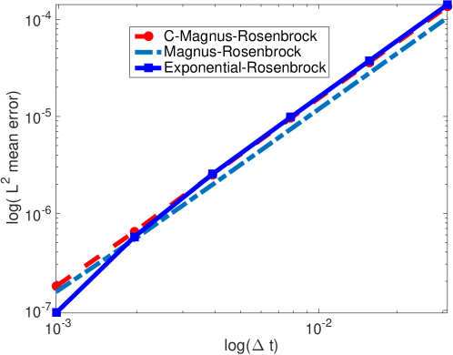
Figure 1: Convergence of the Magnus Rosenbrock scheme at final time $T=1$. For constant coefficient $D(t)=1$, we have compared the Magnus Rosenbrock scheme with the second order exponential Euler Rosenbrock scheme Antjd2 . The order of convergence in time is $1.92$ Magnus Rosenbrock scheme (with $D(t)=1+e^{-t}$), $1.95$ for the Magnus Rosenbrock scheme (with $D(t)=1$)and $2.08$ for the second order exponential Euler Rosenbrock scheme.

In Figure 1, we can observe the convergence of the Magnus Rosenbrock scheme ($D(t)=1+e^{-t}$ and $D(t)=1$), and the second order exponential Euler Rosenbrock scheme ($D(t)=1$). The order of convergence in time is $1.92$ for Magnus Rosenbrock scheme ($D(t)=1+e^{-t}$), $1.95$ for the Magnus Rosenbrock scheme ($D(t)=1$) and $2.08$ for the second order exponential Euler Rosenbrock scheme ($D(t)=1$). As we can also observe, the convergence orders in time of the Magnus Rosenbrock scheme are well in agreement with our theoretical result in Theorem 2.6 as the theoretical order is $2$ with order reduction $\epsilon$, which is very small here.

References

- (1) Amann, H.: On abstract parabolic fundamental solutions. J. Math. Soc. Japan 39, 93-116 (1987)
- (2) Blanes, S., Casa, F., Oteo, J. A., Ros, J.: The Magnus expansion and some of its applications. Physics Reports 470, (2009), 151-238 (2009)
- (3) Blanes, S., Casas, F., Oteo, J. A., Ros, J.: Magnus and Fer expansion for matrix differential equations : the convergence problem. J. Phys. A. : Math. Gen. 31, 259-268 (1998)
- (4) Blanes, S., Moan, P. C.: Fourth- and sixth-order commutator-free Magnus integrators for linear and non-linear dynamical systems. Appl. Numer. Math. 56, 1519-1537 (2006)
- (5) Ciarlet, P. G.: The finite element method for elliptic problems. Amsterdam: North-Holland (1978)
- (6) Elliot, C., Larsson, S., Error estimates with smooth and nonsmooth data for a finite element method for the Cahn-Hilliard equation. Math. Comput. 58, 603-630 (1992)
- (7) Engel, K. J., Nagel, R.: One parameter semigroup for linear evolution equations. Springer New York (2000)
- (8) Evans, L. C.: Partial Differential Equations. Grad. Stud. vol. 19 (1997)
- (9) Fujita, H., Suzuki, T.: Evolutions problems (part1). in: P. G. Ciarlet and J. L. Lions(eds.), Handb. Numer. Anal., vol. II, North-Holland, 789-928 (1991)
- (10) Gondal, M. A.: Exponential Rosenbrock integrators for option pricing. J. Comput. Appl. Math. 234(4), 1153-1160 (2010)
- (11) González, C., Ostermann, A.: Optimal convergence results for Runge-Kutta discretizations of linear nonautonomous parabolic problems, BIT 39(1), 79-95 (1999)
- (12) González, C., Ostermann, A., . Thalhmmer, M.: A second-order Magnus-type integrator for non autonomous parabolic problems. J. Comput. Appl. Math. 189, 142-156 (2006)
- (13) González, C., Ostermann, A., Palencia, C., Thalhammer, M.: Backward Euler discretization of fully nonlinear parabolic problems. Math. Comp. 71, 125-145 (2002)
- (14) González, C., Thalhmmer, M.: A second-order Magnus-type integrator for quasi-linear parabolic problems. Math. Comp. 76(257), 205-231 (2007)
- (15) Hairer, E., Wanner, G.: Solving ordinary differential equations II, stiff and differential-algebraic problems. Second Revisited edition, Springer Series in Computational Mathematics (2000)
- (16) Henry, D.: Geometric Theory of semilinear parabolic equations. Lecture notes in Mathematics, vol. 840, Berlin : Springer (1981)
- (17) Hipp, D., Hochbruck, M., Ostermann, A.: An exponential integrator for non-autonomous parabolic problems. Elect. Trans. Numer. Anal. 41, 497-511 (2014)
- (18) Hochbruck, M., Ostermann, A., Schweitzer, J.: Exponential Rosenbrock-Type methods. SIAM J. Numer. Anal. 47(1) (2009), 786-803
- (19) Hochbruck, M. Lubich, C.: On Magnus integrators for time-dependent Schrödinger equations. SIAM. J. Numer. Anal. 41, 945-963 (2003)
- (20) Hochbruck, M., Ostermann, A.: Exponential integrators. Acta Numerica, 209-286, (2010) doi:10.1017/S0962492910000048
- (21) Iserles, A., Munthe-Kaas, H. Z., Nørsett S. P., Zanna, A.: Lie group methods. Acta Numer. 9, 215-365 (2000)
- (22) Jentzen, A., Kloeden, P. E.: Overcoming the order barrier in the numerical approximation of stochastic partial differential equations with additive space-time noise, Proc. R. Soc. 465, 649-667 (2009)
- (23) Jentzen, A., Kloeden, P. E., Winkel, G.: Efficient simulation of nonlinear parabolic SPDEs with additive noise. Ann. Appl. Prob. 21(3), 908-950 (2011)
- (24) Kloeden, P. E., Platen, E.: Numerical solutions of differential equations. Springer Verlag (1992)
- (25) Larsson, S.: Semilinear parabolic partial differential equations : theory, approximation, and application. In new Trends in the Mathematical and computer sciences, Cent. Math. Comp. Sci. (ICMCS), Lagos, 153-194 (2006)
- (26) Larsson, S.: Nonsmooth data error estimates with applications to the study of the long-time behavior of the finite elements solutions of semilinear parabolic problems. Preprint 6, Departement of Mathematics, Chalmers University of Technology. http://www.math.chalmers.se/∼stig/papers/index.html (1992)
- (27) Leykekhman, D., Vexler, B.: Discrete Maximal parabolic regularity for Galerkin finite element methods for non-autonomous parabolic problems. arXiv: 1707.09163v1 (2017)
- (28) Lord G. J., Tambue, A.: Stochastic exponential integrators for the finite element discretization of SPDEs for multiplicative and additive noise. IMA J. Numer. Anal. 2, 1-29 (2012)
- (29) Lu, Y. Y.: A fourth-order Magnus scheme for Helmholtz equation. J. Compt. Appl. Math. 173, 247-253 (2005)
- (30) Lunardi, A.: Analytic semigroups and optimal regularity in parabolic problems, Birkhäuser, Basel (1995)
- (31) Luskin, M., Rannacher, R.: On the smoothing property of the Galerkin method for parabolic equations. SIAM. J. Numer. Anal. 19(1), 1-21 (1981)
- (32) Magnus, M.: On the exponential solution of a differential equation for a linear operator. Comm. Pure Appl. Math. 7, 649-673 (1954)
- (33) Mingyou. H., Thomee, V.: Some Convergence Estimates for Semidiscrete Type Schemes for Time-Dependent Nonselfadjoint Parabolic Equations. Math. Comp. 37, 327-346 (1981)
- (34) Mukam, J. D., Tambue, A.: Strong convergence analysis of the stochastic exponential Rosenbrock scheme for the finite element discretization of semilinear SPDEs driven by multiplicative and additive noise. J. Sci. Comput. 74, 937-978 (2018)
- (35) Mukam, J. D., Tambue, A.: A note on exponential Rosenbrock-Euler method for the finite element discretization of a semilinear parabolic partial differential equation. In press, Computers and Mathematics with Applications, https://doi.org/10.1016/j.camwa.2018.07.025, 2018.
- (36) Nambu, T.: Characterization of the Domain of Fractional Powers of a Class of Elliptic Differential Operators with Feedback Boundary Conditions. J. Diff. Eq. 136, 294-324 (1997)
- (37) Ostermann, A., Thalhammer, M.: Convergence of Runge-Kutta methods for nonlinear parabolic equations. Appl. Numer. Math. 42, 367-380 (2002)
- (38) Ostermann, A., Thalhammer, M.: Non-smooth data error estimate for linearly implicit Runge-Kutta methods. IMA J. Numer. Anal. 20, 167-184 (2000)
- (39) Pazy, A.: Semigroup of Linear Operators and Applications to Partial Differential Equations. Springer new York (1983)
- (40) Seely, R.: Norms and domains of the complex powers . Amer. J. Math. 93, 299-309 (1971)
- (41) Seidler, J.: Da Prato-Zabczyk’s maximal inequality revisited I. Math. Bohem. 118(1), 67-106 (1993)
- (42) Tambue, A., Lord G. J, Geiger, S.: An exponential integrator for advection-dominated reactive transport in heterogeneous porous media. Journal of Computational Physics, 229(10), 3957–3969 (2010)
- (43) Tambue, A., Ngnotchouye, J. M. T.: Weak convergence for a stochastic exponential integrator and finite element discretization of stochastic partial differential equation with multiplicative & additive noise. Appl. Numer. Math. 108, 57-86 (2016)
- (44) Tanabe, H.: Equations of Evolutions. Pitman London (1979)
- (45) Caliari,M., Vianello M., Bergamaschi L. The LEM exponential integrator for advection–diffusion–reaction equations. Journal of Computational and Applied Mathematics, 210, 56– 63 (2007)
- (46) Thomée, V.: Galerkin finite element method for parabolic problems, 2edn. Springer Series in Computational Mathematics, vol. 25. Berlin: Springer (2006)