Exploring dark matter, neutrino mass and $R_{K^{(*)},\phi}$ anomalies in $L_{\mu}-L_{\tau}$ model

Abstract

We investigate Majorana dark matter in a new variant of $U(1)_{L_{\mu}-L_{\tau}}$ gauge extension of Standard Model, where the scalar sector is enriched with an inert doublet and a $(\bar{3},1,1/3)$ scalar leptoquark. We compute the WIMP-nucleon cross section in leptoquark portal and the relic density mediated by inert doublet components, leptoquark and the new $Z^{\prime}$ boson. We constrain the parameter space consistent with Planck limit on relic density, PICO-60 and LUX bounds on spin-dependent direct detection cross section. Furthermore, we constrain the new couplings from the present experimental data on ${\rm Br}(\tau\to\mu\nu_{\tau}\bar{\nu}_{\mu})$, ${\rm Br}(B\to X_{s}\gamma)$, ${\rm Br}(\bar{B}^{0}\to\bar{K}^{0}\mu^{+}\mu^{-})$, ${\rm Br}(B^{+}\to K^{+}\tau^{+}\tau^{-})$ and $B_{s}-\bar{B_{s}}$ mixing, which occur at one-loop level in the presence of $Z^{\prime}$ and leptoquark. Using the allowed parameter space, we estimate the form factor independent $P_{4,5}^{\prime}$ observables and the lepton non-universality parameters $R_{K}$, $R_{K^{*}}$ and $R_{\phi}$. We also briefly discuss about the neutrino mass generation at one-loop level and the viable parameter region to explain current neutrino oscillation data.

I Introduction

Though the experimental measured values of various physical observables are in excellent agreement with the Standard Model (SM) predictions, there are many open unsolved problems like the matter-antimatter asymmetry, hierarchy problem and the dark matter (DM) content of the universe etc., which make ourselves believe that there is something beyond the SM. In this regard, the study of rare semileptonic $B$ decay processes provide an ideal testing ground to critically test the SM and to look for possible extension of it. Although, so far we have not observed any clear indication of new physics (NP) in the $B$ sector, there are several physical observables associated with flavor changing neutral current (FCNC) $b\to sl^{+}l^{-}$ processes which have $(2-4)\sigma$ Aaij et al. (2017, 2014a, 2013a, 2013b, 2014b); Langenbruch (2015) discrepancies. Especially, the observation of $3\sigma$ anomaly in the $P_{5}^{\prime}$ angular observables Aaij et al. (2013b) and the decay rate Aaij et al. (2014b) of $B^{0}\to K^{*0}\mu^{+}\mu^{-}$ processes have attracted a lot of attention in recent times. The decay rate of $B_{s}\to\phi\mu^{+}\mu^{-}$ has also $3\sigma$ deviation compared to its SM prediction Aaij et al. (2013a). Furthermore, the LHCb Collaboration has observed the violation of lepton universality in $B^{+}\to K^{+}l^{+}l^{-}$ process in the low $q^{2}\in[1,6]~{}{\rm GeV}^{2}$ region Aaij et al. (2014a)

$$R_{K}^{\rm Expt}=\frac{{\rm Br}(B^{+}\to K^{+}\mu^{+}\mu^{-})}{{\rm Br}(B^{+}\to K^{+}e^{+}e^{-})}=0.745^{+0.090}_{-0.074}\pm 0.036,$$ (1)

which has a $2.6\sigma$ deviation from the corresponding SM result Bobeth et al. (2007)

$$R_{K}^{\rm SM}=1.0003\pm 0.0001.$$ (2)

In addition, an analogous lepton non-universality (LNU) parameter $(R_{K^{*}})$ has also been observed in $B^{0}\to K^{*0}l^{+}l^{-}$ processes Aaij et al. (2017)

$$R_{K^{*}}^{\rm Expt}=\frac{{\rm Br}(B^{0}\to K^{*0}\mu^{+}\mu^{-})}{{\rm Br}(B^{0}\to K^{*0}e^{+}e^{-})} = 0.66^{+0.11}_{-0.07}\pm 0.03,~{}~{}~{}~{}q^{2}\in[0.045,1.1]~{}{\rm GeV}^{2},$$ (3)

$$= 0.69^{+0.11}_{-0.07}\pm 0.05,~{}~{}~{}~{}q^{2}\in[1.1,6]~{}{\rm GeV}^{2},$$

which correspond to the deviation of $2.2\sigma$ and $2.4\sigma$ from their SM predictions Capdevila et al. (2018)

$$R_{K^{*}}^{\rm SM}\big{|}_{q^{2}\in[0.045,1.1]~{}{\rm GeV^{2}}}=0.92\pm 0.02,~{}~{}~{}~{}R_{K^{*}}^{\rm SM}\big{|}_{q^{2}\in[1.1,6]~{}{\rm GeV^{2}}}=1.00\pm 0.01.$$ (4)

To resolve the above $b\to sll$ anomalies, we extend the SM gauge group $SU(3)_{C}\times SU(2)_{L}\times U(1)_{Y}$ with a local $U(1)_{L_{\mu}-L_{\tau}}$ symmetry. The anomaly free $L_{\mu}-L_{\tau}$ gauge extensions He et al. (1991a, b) are captivating with minimal new particles and parameters, rich in phenomenological perspective. The model is quite simple in structure, suitable to study the phenomenology of DM, neutrino and also the flavor anomalies Crivellin et al. (2015a); Patra et al. (2017); Biswas et al. (2016); Kamada et al. (2018); Bauer et al. (2018). It is well explored in dark matter context in literature Patra et al. (2017); Biswas et al. (2016); Kamada et al. (2018); Bauer et al. (2018), in the gauge and scalar portals. In the literature Crivellin et al. (2015b); Das et al. (2017, 2018a, 2018b), the DM, neutrino and flavor phenomenology are also investigated in several $U(1)$ extended models. The approach of adding color triplet particles to shed light on the flavor sector thereby connecting with dark sector is interesting. Leptoquarks (LQ) are not only advantageous in addressing the flavor anomalies, but also act as a mediator between the visible and dark sector. Few works were already done with this motivation Baek (2018); Mandal (2018); Arcadi et al. (2017); Allahverdi et al. (2018).

Leptoquarks are hypothetical color triplet gauge particles, with either spin-0 (scalar) or spin-1 (vector), which connect the quark and lepton sectors and thus, carry both baryon and lepton numbers simultaneously. They can arise from various extended standard model scenarios Georgi and Glashow (1974); Georgi (1975); Langacker (1981); Fritzsch and Minkowski (1975); Pati and Salam (1974, 1973a, 1973b); Shanker (1982a, b); Schrempp and Schrempp (1985); Gripaios (2010); Kaplan (1991), which treat quarks and leptons on equal footing, such as the grand unified theories (GUTs) Georgi and Glashow (1974); Fritzsch and Minkowski (1975); Langacker (1981); Georgi (1975), color $SU(4)$ Pati-Salam model Pati and Salam (1974, 1973a, 1973b); Shanker (1982a, b), extended technicolor model Schrempp and Schrempp (1985); Gripaios (2010) and the composite models of quark and lepton Kaplan (1991). In this article, we study a new version of $U(1)_{L_{\mu}-L_{\tau}}$ gauge extension of SM with a $(\bar{3},1,1/3)$ scalar LQ (SLQ) and an inert doublet, to study the phenomenology of dark matter, neutrino mass generation and compute the flavor observables on a single platform. The SLQ mediates the annihilation channels contributing to relic density and also plays a crucial role in direct searches as well, providing a spin-dependent WIMP-nucleon cross section which is quite sensitive to the recent and ongoing direct detection experiments such as PICO-60 and LUX. The $Z^{\prime}$ gauge boson of extended $U(1)$ symmetry and the SLQ also play an important role in settling the known issues of flavor sector. In this regard, we would like to investigate whether the observed anomalies in the rare leptonic/semileptonic decay processes mediated by $b\to sl^{+}l^{-}$ transitions, can be explained in the present framework. We analyze the implications of the model on both the DM and flavor sectors, in particular on $B\to Vl^{+}l^{-}~{}(V=K^{*},\phi)$ decay modes. In literature Alok et al. (2017); Bečirević and Sumensari (2017); Hiller and Nisandzic (2017); D’Amico et al. (2017); Bečirević et al. (2016); Bauer and Neubert (2016); Li et al. (2016); Calibbi et al. (2015); Freytsis et al. (2015); Dumont et al. (2016); Doršner et al. (2016); de Medeiros Varzielas and Hiller (2015); Dorsner et al. (2011); Davidson et al. (1994); Saha et al. (2010); Mohanta (2014); Sahoo and Mohanta (2016a, b, c, 2015); Kosnik (2012); Chauhan et al. (2018); Bečirević et al. (2018); Angelescu et al. (2018), there were many attempts being made to explain the observed anomalies of rare $B$ decays in the scalar leptoquark model.

The paper is structured as follows. We describe the particle content, relevant Lagrangian and interaction terms, pattern of symmetry breaking in section-II. We derive the mass eigenstates of the new fermions and the scalar spectrum in section-III. We then provide a detailed study of DM phenomenology in prospects of relic density and direct detection observables in section-IV. The mechanism of generating light neutrino mass at one-loop level, consistent with the current oscillation data is illustrated in section V. Section-VI contains the additional constraint on the new parameters obtained from the existing anomalies of the flavor sector, like ${\rm Br}(\tau\to\mu\nu_{\tau}\bar{\nu}_{\mu})$, ${\rm Br}(B\to X_{s}\gamma)$, ${\rm Br}(\bar{B}^{0}\to\bar{K}^{0}\mu^{+}\mu^{-})$, ${\rm Br}(B^{+}\to K^{+}\tau\tau)$ and $B_{s}-\bar{B_{s}}$ mixing. We then investigate the impact of additional $U(1)_{L_{\mu}-L_{\tau}}$ gauge symmetry on the $R_{K^{(*)}}$, $R_{\phi}$ LNU parameters and optimized $P_{4,5}^{\prime}$ observables in section-VII. We summarize our findings in Section-VIII.

II New $L_{\mu}-L_{\tau}$ model with a scalar leptoquark

We study the well known anomaly free $U(1)_{L_{\mu}-L_{\tau}}$ extension of SM containing three additional neutral fermions $N_{e},N_{\mu},N_{\tau}$, with $L_{\mu}-L_{\tau}$ charges $0,1$ and $-1$ respectively. A scalar singlet $\phi_{2}$, charged $+2$ under the new $U(1)$ is added to spontaneously break the local $U(1)_{L_{\mu}-L_{\tau}}$ gauge symmetry. We also introduce an inert doublet $\eta$ and a scalar leptoquark $S_{1}(\bar{3},1,1/3)$ with $L_{\mu}-L_{\tau}$ charges $0$ and $-1$ to the scalar content of the model. We impose an additional $Z_{2}$ symmetry under which all the new fermions, $\eta$ and the leptoquark are odd and rest are even. The particle content and their corresponding charges are displayed in Table. 1 .

	Field	$SU(3)_{C}\times SU(2)_{L}\times U(1)_{Y}$	$U(1)_{L_{\mu}-L_{\tau}}$	$Z_{2}$
Fermions	$Q_{L}\equiv(u,d)^{T}_{L}$	$(\textbf{3},\textbf{2},~{}1/6)$	$0$	$+$
	$u_{R}$	$(\textbf{3},\textbf{1},~{}2/3)$	$0$	$+$
	$d_{R}$	$(\textbf{3},\textbf{1},~{}-1/3)$	$0$	$+$
	$e_{L}\equiv(\nu_{e},~{}e)^{T}_{L}$	$(\textbf{1},\textbf{2},~{}-1/2)$	$0$	$+$
	$e_{R}$	$(\textbf{1},\textbf{1},~{}-1)$	$0$	$+$
	$\mu_{L}\equiv(\nu_{\mu},~{}\mu)^{T}_{L}$	$(\textbf{1},\textbf{2},~{}-1/2)$	$1$	$+$
	$\mu_{R}$	$(\textbf{1},\textbf{1},~{}-1)$	$1$	$+$
	$\tau_{L}\equiv(\nu_{\tau},~{}\tau)^{T}_{L}$	$(\textbf{1},\textbf{2},~{}-1/2)$	$-1$	$+$
	$\tau_{R}$	$(\textbf{1},\textbf{1},~{}-1)$	$-1$	$+$
	$N_{e}$	$(\textbf{1},\textbf{1},~{}0)$	$0$	$-$
	$N_{\mu}$	$(\textbf{1},\textbf{1},~{}0)$	$1$	$-$
	$N_{\tau}$	$(\textbf{1},\textbf{1},~{}0)$	$-1$	$-$
Scalars	$H$	$(\textbf{1},\textbf{2},~{}1/2)$	$0$	$+$
	$\eta$	$(\textbf{1},\textbf{2},~{}1/2)$	$0$	$-$
	$\phi_{2}$	$(\textbf{1},\textbf{1},~{}0)$	$2$	$+$
	$S_{1}$	$(\bar{\textbf{3}},\textbf{1},~{}1/3)$	$-1$	$-$

Table 1: Fields and their charges of the proposed $U(1)_{L_{\mu}-L_{\tau}}$ model.

The Lagrangian of the present model can be written as

$${\cal L} ={\cal L}_{\rm SM}-{1\over 4}Z^{\prime}_{\mu\nu}Z^{{}^{\prime}\mu\nu}-g_{\mu\tau}\overline{\mu}_{L}\gamma^{\mu}\mu_{L}Z_{\mu}^{\prime}-g_{\mu\tau}\overline{\mu}_{R}\,\gamma^{\mu}\mu_{R}Z_{\mu}^{\prime}+g_{\mu\tau}\overline{\tau}_{L}\gamma^{\mu}\tau_{L}Z_{\mu}^{\prime}+g_{\mu\tau}\overline{\tau}_{R}\,\gamma^{\mu}\tau_{R}Z_{\mu}^{\prime}$$

$$+\overline{N}_{e}i\not{\partial}\,N_{e}+\overline{N}_{\mu}\left(i\not{\partial}-g_{\mu\tau}\,Z_{\mu}^{\prime}\gamma^{\mu}\right)N_{\mu}+\overline{N}_{\tau}\left(i\not{\partial}+g_{\mu\tau}\,Z_{\mu}^{\prime}\gamma^{\mu}\right)N_{\tau}-\frac{f_{\mu}}{2}\left({\overline{N_{\mu}^{c}}}N_{\mu}\phi_{2}^{\dagger}+{\rm h.c.}\right)$$

$$-\frac{f_{\tau}}{2}\left({\overline{N_{\tau}^{c}}}N_{\tau}\phi_{2}+{\rm h.c.}\right)-\frac{1}{2}M_{ee}\overline{N_{e}^{c}}N_{e}-\frac{1}{2}M_{\mu\tau}(\overline{N_{\mu}^{c}}N_{\tau}+\overline{N_{\tau}^{c}}N_{\mu})-\sum_{q=d,s,b}(y_{qR}\;\overline{d_{qR}^{c}}S_{1}N_{\mu}+{\rm{h.c.}})$$

$$-\sum_{l=e,\mu,\tau}(Y_{\beta l}(\overline{\ell_{L}})_{\beta}\tilde{\eta}N_{lR}+{\rm{h.c}})+\left|\left(i\partial_{\mu}-\frac{g}{2}\boldsymbol{\tau}^{a}\cdot\mathbb{W}_{\mu}^{a}-\frac{g^{\prime}}{2}B_{\mu}\right)\eta\right|^{2}+\left|\left(i\partial_{\mu}-\frac{g^{\prime}}{3}B_{\mu}+g_{\mu\tau}\,Z_{\mu}^{\prime}\right)S_{1}\right|^{2}$$

$$+\left|\left(i\partial_{\mu}-2g_{\mu\tau}\,Z_{\mu}^{\prime}\right)\phi_{2}\right|^{2}-V(H,\eta,\phi_{2},S_{1}),$$ (5)

where the scalar potential $V$ is

$$V(H,\eta,\phi_{2},S_{1}) =\mu^{2}_{H}H^{\dagger}H+\lambda_{H}(H^{\dagger}H)^{2}+\mu_{\eta}(\eta^{\dagger}\eta)+\lambda_{H\eta}(H^{\dagger}H)(\eta^{\dagger}\eta)+\lambda_{\eta}(\eta^{\dagger}\eta)^{2}+\lambda^{\prime}_{H\eta}(H^{\dagger}\eta)(\eta^{\dagger}H)$$

$$+ \frac{\lambda^{\prime\prime}_{H\eta}}{2}\left[(H^{\dagger}\eta)^{2}+{\rm h.c.}\right]+\mu^{2}_{2}(\phi^{\dagger}_{2}\phi_{2})+\lambda_{2}(\phi^{\dagger}_{2}\phi_{2})^{2}+\mu^{2}_{S}({S_{1}}^{\dagger}{S_{1}})+\lambda_{S}({S_{1}}^{\dagger}{S_{1}})^{2}$$

$$+ \left[\lambda_{H2}(\phi^{\dagger}_{2}\phi_{2})+\lambda_{HS}(S^{\dagger}_{1}S_{1})\right](H^{\dagger}H)+\lambda_{S2}(\phi^{\dagger}_{2}\phi_{2})({S_{1}}^{\dagger}{S_{1}})+\lambda_{\eta 2}(\phi^{\dagger}_{2}\phi_{2})(\eta^{\dagger}\eta)$$

$$+ \lambda_{S\eta}({S_{1}}^{\dagger}S_{1})(\eta^{\dagger}\eta).$$ (6)

The gauge symmetry $SU(2)_{L}\times U(1)_{Y}\times U(1)_{L_{\mu}-L_{\tau}}$ is spontaneously broken to $SU(2)_{L}\times U(1)_{Y}$ by assigning a VEV $v_{2}$ to the complex singlet $\phi_{2}$. Then the SM Higgs doublet breaks the SM gauge group to low energy theory by obtaining a VEV $v$. The new neutral gauge boson $Z^{\prime}$ associated with the $U(1)$ extension absorbs the massless pseudoscalar in $\phi_{2}$ to become massive. The neutral components of the fields $H$ and $\phi_{2}$ can be written in terms of real scalars and pseudoscalars as

$$H^{0}=\frac{1}{\sqrt{2}}(v+h)+\frac{i}{\sqrt{2}}A^{0}\,,$$

$$\phi_{2}=\frac{1}{\sqrt{2}}(v_{2}+h_{2})+\frac{i}{\sqrt{2}}A_{2}\,.$$ (7)

The inert doublet is denoted by $\eta=\begin{pmatrix}\eta^{+}\\ \eta^{0}\\ \end{pmatrix}$, with $\eta^{0}=\displaystyle{\frac{\eta_{e}+i\eta_{o}}{\sqrt{2}}}$. The masses of its charged and neural components are given by

$$M_{\eta^{+}}^{2} = \mu_{\eta}^{2}+\frac{\lambda_{H\eta}}{2}v^{2}+\frac{\lambda_{\eta 2}}{2}v^{2}_{2}\;,$$

$$M_{\eta_{e}}^{2} = \mu_{\eta}^{2}+\frac{\lambda_{\rm\eta 2}}{2}v^{2}_{2}+\left(\lambda_{H\eta}+\lambda^{\prime}_{H\eta}+\lambda^{\prime\prime}_{H\eta}\right)\frac{v^{2}}{2}\;,$$

$$M_{\eta_{o}}^{2} = \mu_{\eta}^{2}+\frac{\lambda_{\rm\eta 2}}{2}v^{2}_{2}+\left(\lambda_{H\eta}+\lambda^{\prime}_{H\eta}-\lambda^{\prime\prime}_{H\eta}\right)\frac{v^{2}}{2}.$$ (8)

The masses obtained by the colored scalar and the gauge boson $Z^{\prime}$ are

$$M_{S_{1}}^{2} = 2\mu_{S}^{2}+\lambda_{HS}v^{2}+\lambda_{S2}v_{2}^{2}\;,$$

$$M_{Z^{\prime}} = 2v_{2}g_{\mu\tau}.$$ (9)

In the whole discussion of the results, we consider the benchmark values for the masses of the scalar spectrum as $(M_{S_{1}},M_{\eta^{+}},M_{\eta_{e,o}})=(1.2,2,1.5)$ TeV.

III Mixing in the fermion and scalar sector

The fermion and scalar mass matrices take the form

$$M_{N}=\begin{pmatrix}\frac{1}{\sqrt{2}}f_{\mu}v_{2}&M_{\mu\tau}\\ M_{\mu\tau}&\frac{1}{\sqrt{2}}f_{\tau}v_{2}\\ \end{pmatrix}\;,\quad M_{S}=\begin{pmatrix}2\lambda_{H}v^{2}&{\lambda}_{H2}{v}v_{2}\\ {\lambda}_{H2}{v}v_{2}&2\lambda_{2}v^{2}_{2}\\ \end{pmatrix}\;.$$ (10)

One can diagonalize the above mass matrices by $U_{\alpha(\zeta)}^{T}M_{N(S)}U_{\alpha(\zeta)}={\rm{diag}}~{}[M_{N_{-}(H_{1})},M_{N_{+}(H_{2})}]$, where

$$U_{\theta}=\begin{pmatrix}\cos{\theta}&\sin{\theta}\\ -\sin{\theta}&\cos{\theta}\\ \end{pmatrix},$$ (11)

with $\zeta=\frac{1}{2}\tan^{-1}\left(\displaystyle{\frac{\lambda_{H2}vv_{2}}{\lambda_{2}v^{2}_{2}-\lambda_{H}v^{2}}}\right)$ and $\alpha=\frac{1}{2}\tan^{-1}\left(\displaystyle{\frac{2M_{\mu\tau}}{(f_{\tau}-f_{\mu})(v_{2}/\sqrt{2})}}\right)$.

We denote the scalar mass eigenstates as $H_{1}$ and $H_{2}$, with $H_{1}$ is assumed to be observed Higgs at LHC with $M_{H_{1}}=125.09$ GeV and $v=246$ GeV. The mixing parameter $\zeta$ is taken minimal to stay with LHC limits on Higgs decay width. We indicate $N_{-}$ and $N_{+}$ to be the fermion mass eigenstates, with the lightest one ($N_{-}$) as the probable dark matter candidate in the present work.

IV Dark matter phenomenology

IV.1 Relic abundance

The model allows the dark matter ($N_{-}$) to have gauge and scalar mediated annihilation channels. The possible contributing diagrams are provided in Fig. 1 which are mediated by $(H_{1},H_{2},\eta^{+},\eta^{0},S_{1},Z^{\prime})$. Majorana DM in $H_{1,2}$ portal (upper row in Fig. 1 ) has already been well explored in literature Singirala et al. (2017); Nanda and Borah (2017). Here, we focus on $(Z^{\prime},S_{1},\eta)$-mediated channels (middle and bottom rows in Fig. 1 ) contributing to DM observables, which we later make connection with radiative neutrino mass as well as flavor observables.

Figure 1: Feynman diagrams contributing to relic density.

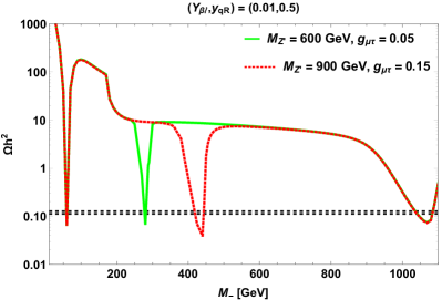
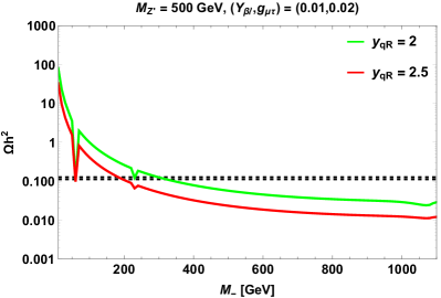
Figure 2: Behavior of relic density plotted against DM mass with $M_{H_{2}}=2.2$ TeV, shown with varying $M_{Z^{\prime}}$ and $g_{\mu\tau}$ (left panel) and $y_{qR}$ (right panel). Black horizontal dotted lines denote the $3\sigma$ range of Planck limit (Aghanim et al., 2018).

The relic abundance of dark matter is computed by

$$\Omega h^{2}=\frac{1.07\times 10^{9}~{}{\rm{GeV}}^{-1}}{M_{\rm{Pl}}\;{g_{\ast}}^{1/2}}\frac{1}{J(x_{f})}\;.$$ (12)

Here the Planck mass, $M_{\rm{Pl}}=1.22\times 10^{19}~{}\rm{GeV}$ and $g_{\ast}=106.75$ denotes the total number of effective relativistic degrees of freedom. The function $J(x_{f})$ reads as

$$J(x_{f})=\int_{x_{f}}^{\infty}\frac{\langle\sigma v\rangle(x)}{x^{2}}dx.$$ (13)

The thermally averaged annihilation cross section $\langle\sigma v\rangle$ is given by the expression

$$\langle\sigma v\rangle(x)=\frac{x}{8M_{-}^{5}K_{2}^{2}(x)}\int_{4M_{-}^{2}}^{\infty}\hat{\sigma}\times(s-4M_{-}^{2})\ \sqrt{s}\ K_{1}\left(\frac{x\sqrt{s}}{M_{-}}\right)ds,$$ (14)

where $K_{1}$, $K_{2}$ denote the modified Bessel functions, $x=M_{-}/T$, with $T$ is the temperature and $\hat{\sigma}$ is the dark matter annihilation cross section. The analytical expression for the freeze out parameter $x_{f}$ is

$$x_{f}=\ln\left(\frac{0.038\ g\ M_{\text{Pl}}\ M_{-}\ \langle\sigma v\rangle(x_{f})}{({g_{\ast}x_{f}})^{1/2}}\right).$$ (15)

Here $g$ represents the number of degrees of freedom of the dark matter particle $N_{-}$.

As seen from the left panel of Fig. 2, the relic density with $s$-channel contribution is featured to meet the Planck limit (Aghanim et al., 2018) near the resonance in propagator ($H_{1},H_{2},Z^{\prime}$), i.e., near $M_{-}=\frac{M_{\rm prop}}{2}$. We restrict our discussion to the mass region (in GeV), $100\leq M_{Z^{\prime}}\leq 1000$, $80\leq M_{-}\leq 1000$ and also $H_{2}$ is considered to be sufficiently large such that its resonance doesn’t meet the Planck limit below $1$ TeV region of DM mass. Now, in this mass range of DM, the channels mediated by $(Z^{\prime},\eta,S_{1})$ drive the relic density observable, where the gauge coupling $g_{\mu\tau}$ controls the $s$-channel contribution, while $Y_{\beta l},~{}y_{qR}$ are relevant in $t$-channel contributions. Hence, the relevant parameters in our investigation are $(M_{-},g_{\mu\tau},M_{Z^{\prime}},Y_{\beta l},y_{qR})$. The effect of these parameters on the relic abundance is made transparent in Fig. 2 , where we have considered $Y_{\beta l}\sim 10^{-2}$, in order to explain neutrino mass at one loop level. Left panel shows the variation of relic density with varying gauge parameters $g_{\mu\tau}$ and $M_{Z^{\prime}}$, right panel depicts the behavior with varying $y_{qR}$ parameter. No significant constraint on $M_{Z^{\prime}}$, $g_{\mu\tau}$ parameters is observed, however relic density has an appreciable footprint on $M_{-}-(y_{qR})^{2}$ parameter space, which will be discussed in the next section.

IV.2 Direct searches

Moving to direct searches, the $Z^{\prime}$ mediated WIMP-nucleon interaction is not possible at tree-level as the $Z^{\prime}$ boson does not couple to quarks. The $t$-channel scalar ($H_{1},H_{2}$) exchange can give spin-independent (SI) contribution, but it doesn’t help our purpose of study. In the scalar portal, one can obtain contribution from spin-dependent (SD) interaction mediated by SLQ, of the form

$$\mathcal{L^{\rm SD}_{\rm eff}}\simeq\frac{y_{qR}^{2}\cos^{2}\alpha}{4(M_{S_{1}}^{2}-M_{-}^{2})}\overline{N_{-}}\gamma^{\mu}\gamma^{5}N_{-}\overline{q}\gamma_{\mu}\gamma^{5}q\,.$$ (16)

The s-channel process is depicted in the left most panel of Fig. 3 and the corresponding cross section is given by Agrawal et al. (2010)

$$\sigma_{\rm SD}=\frac{\mu_{r}^{2}}{\pi}\frac{\cos^{4}\alpha}{(M_{S_{1}}^{2}-M_{-}^{2})^{2}}\left[y_{dR}^{2}\Delta_{d}+y_{sR}^{2}\Delta_{s}\right]^{2}J_{n}(J_{n}+1),$$ (17)

where the angular momentum $J_{n}=\frac{1}{2}$, reduced mass $\mu_{r}=\frac{M_{-}M_{n}}{M_{-}+M_{n}}$ with $M_{n}\simeq 1$ GeV for nucleon. The values of quark spin functions $\Delta_{q}$ are provided in (Agrawal et al., 2010). Now, it is obvious that it can constrain the parameters $M_{-}$ and $(y_{qR})^{2}$. Fig. 4, left panel displays $M_{-}-(y_{qR}^{2})$ parameter space (green and red regions) remained after imposing Planck Aghanim et al. (2018) $3\sigma$ limit on current relic density. Here, the region shown in green turns out to be excluded by most stringent PICO-60 Amole et al. (2017) limit on SD WIMP-proton cross section, as seen from the right panel.

Figure 3: Diagrams involving SLQ relevant in direct detection study.

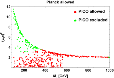
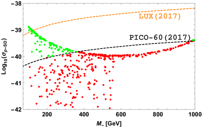
Figure 4: Left panel depicts the $M_{-}-(y_{qR})^{2}$ parameter space consistent upto $3\sigma$ level of Planck limit (Aghanim et al., 2018) on relic density. Right panel gives the SD WIMP-proton cross section as a function of DM mass. Dashed lines represent the recent bounds obtained from PICO-60 Amole et al. (2017) and LUX Akerib et al. (2017a). Green (red) data points in both the panels represent Planck allowed and PICO excluded (Planck and PICO allowed).

Apart from tree-level, one-loop penguin diagrams (middle and right panels of Fig. 3) involving SLQ, mediated by SM neutral gauge boson ($Z$) and the neutral scalars ($H_{1},H_{2}$) can provide SD and SI contributions respectively. The effective interaction Lagrangian relevant for SD cross section is given by Ibarra et al. (2016); Herrero-Garcia et al. (2018)

$$\mathcal{L^{\rm SD-loop}_{\rm eff}}\simeq\xi_{q^{\prime}}\overline{N_{-}}\gamma^{\mu}\gamma^{5}N_{-}\overline{q^{\prime}}\gamma_{\mu}\gamma^{5}q^{\prime}\,,$$ (18)

where

$$\xi_{q^{\prime}}=\sum_{q=d,s,b}\frac{y_{qR}^{2}\cos^{2}\alpha~{}a_{q^{\prime}}}{32\pi^{2}M_{Z}^{2}}\left[(v_{q}+a_{q})G\left(\frac{M_{-}^{2}}{M_{S_{1}}^{2}}\right)\right]\,.$$ (19)

And the loop function takes the form

$$G(x)=-1+\frac{2\left(x+(1-x){\rm{ln}}(1-x)\right)}{x^{2}}\,.$$ (20)

The corresponding WIMP-nucleon cross section is given by

$$\sigma^{\rm loop}_{\rm SD}=\frac{16\mu_{r}^{2}}{\pi}J_{n}(J_{n}+1)(\xi_{u}\Delta_{u}+\xi_{d}\Delta_{d}+\xi_{s}\Delta_{s})^{2}\,.$$ (21)

In the above expression, $v_{q}=\displaystyle{\frac{g}{2\cos\theta_{w}}}\left(-\frac{1}{2}+\frac{2}{3}\sin^{2}\theta_{w}\right)$, $a_{q}=-\displaystyle{\frac{g}{4\cos\theta_{w}}}$ and $a_{q^{\prime}}=\displaystyle{\frac{g}{4\cos\theta_{w}}}\left(-\displaystyle{\frac{g}{4\cos\theta_{w}}}\right)$ for $q^{\prime}=u~{}(d,s)$. For SI contribution, the effective interaction term is

$$\mathcal{L^{\rm SI-loop}_{\rm eff}}\simeq\Lambda_{q^{\prime}}\overline{N_{-}}N_{-}\overline{q^{\prime}}q^{\prime}\,.$$ (22)

and the corresponding cross-section are given by

$$\sigma^{\rm loop}_{\rm SI}=\frac{4\mu_{r}^{2}}{\pi}M_{n}^{2}\left(\frac{\Lambda_{q^{\prime}}}{m_{q^{\prime}}}\right)^{2}f_{n}^{2}\;,$$ (23)

where

$$\Lambda_{q^{\prime}}=-\sum_{q=d,s,b}\frac{y_{qR}^{2}\cos^{2}\alpha}{16\pi^{2}}\left[\frac{\lambda_{HS}v\cos\zeta-\lambda_{S2}v_{2}\sin\zeta}{M_{H_{1}}^{2}}+\frac{\lambda_{HS}v\sin\zeta+\lambda_{S2}v_{2}\cos\zeta}{M_{H_{2}}^{2}}\right]G_{1}\left(\frac{M_{-}^{2}}{M_{S_{1}}^{2}}\right)\frac{m_{q^{\prime}}}{vM_{-}}\,.$$

Here $\displaystyle{G_{1}(x)=\frac{x+(1-x){\rm{ln}}(1-x)}{x}}$. For proton, the typical value of the scalar form factor $f_{n}$ is $\sim 0.3$. Fig. 5, left and right panels project the one-loop SD and SI contributions respectively for the parameter space consistent with Planck data. We see that these contributions are well below the current upper limits set by direct detection collaborations such as PICO-60 Amole et al. (2017), LUX Akerib et al. (2017a) for SD and PandaX-II Cui et al. (2017), XENON1T Aprile et al. (2017), LUX Akerib et al. (2017b) for SI cases. Thus they do not have any impact on the range of model parameters.

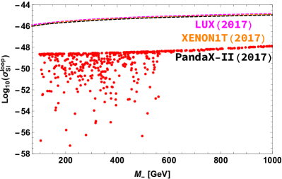
Figure 5: One-loop SD and SI contributions projected in the left and right panels respectively. Stringent upper limits of PICO-60 Amole et al. (2017) and LUX Akerib et al. (2017a) are given in the left panel, PandaX-II Cui et al. (2017), XENON1T Aprile et al. (2017) and LUX Akerib et al. (2017b) bounds are provided in the right panel.

V Radiative neutrino mass

The light neutrino mass can be generated at one-loop level from the Yukawa interaction with inert doublet in Eqn. 5. and the corresponding diagram is shown in Fig. 6 . Assuming $m_{0}^{2}=(M^{2}_{\eta_{e}}+M^{2}_{\eta_{o}})/{2}$ is much greater than $M^{2}_{\eta_{e}}-M^{2}_{\eta_{o}}=\lambda^{\prime\prime}_{H\eta}v^{2},$ the expression for the radiatively generated neutrino mass Ma (2006) is given by

$$({\cal M}_{\nu})_{\beta\gamma}={\lambda^{\prime\prime}_{H\eta}v^{2}\over 16\pi^{2}}\sum_{l=e,\mu,\tau}{Y_{\beta l}Y_{\gamma l}M_{Dl}\over m_{0}^{2}-M^{2}_{Dl}}\left[1+{M^{2}_{Dl}\over m_{0}^{2}-M^{2}_{Dl}}\ln{M^{2}_{Dl}\over m_{0}^{2}}\right].$$ (24)

Here $M_{Dl}=(U^{T}M_{N}U)_{l}={\rm diag}(M_{ee},M_{-},M_{+})$ and the fermion mass eigenstates $N_{Dl}=U^{\dagger}_{lm}N_{m}$. The light neutrino mass matrix (24) can be expressed as

$$({\cal M}_{\nu})_{\beta\gamma}\equiv(Y^{T}\Lambda Y)_{\beta\gamma}\;,$$ (25)

where the matrix $\Lambda$ is defined as $\Lambda={\rm diag}(\Lambda_{1},\Lambda_{2},\Lambda_{3})$, with

$$\Lambda_{l}={\lambda^{\prime\prime}_{H\eta}v^{2}\over 16\pi^{2}}{M_{Dl}\over m_{0}^{2}-M^{2}_{Dl}}\left[1+{M^{2}_{Dl}\over m_{0}^{2}-M^{2}_{Dl}}\ln{M^{2}_{Dl}\over m_{0}^{2}}\right].$$ (26)

Generation-wise, the $L_{\mu}-L_{\tau}$ charges of SM leptons match with the charges of new fermions $N_{l}$ ($0,+1,-1$ respectively). The Yukawa interaction term is written using an inert doublet $\eta$ with vanishing $L_{\mu}-L_{\tau}$ charge, and thus the Yukawa matrix $Y_{\beta l}$ takes diagonal form. Hence, the neutrino mass matrix (25) is diagonal, by model construction i.e., ${\cal M}_{\nu}={\rm diag}(M_{1},M_{2},M_{3})$. In order to find the viable region for model parameters consistent with the current neutrino oscillation data, i.e., $6.93\leq\Delta M_{\rm sol}^{2}~{}[{10^{-5}}\;{\rm eV^{2}}]\leq 7.97$, $2.37\leq\Delta M_{\rm atm}^{2}~{}[{10^{-3}}\;{\rm eV^{2}}]\leq 2.63$ Capozzi et al. (2016), and cosmological bound on the sum of the light neutrino mass, $\sum_{i}M_{i}<0.23$ eV Ade et al. (2016), we perform a scan by varying the parameters in the following range (where the masses are considered in GeV):

$$1000\leq M_{ee}\leq 3000,~{}~{}~{}100\leq M_{-}\leq 1000,~{}~{}~{}2000\leq M_{+}\leq 5000,~{}~{}~{}1000\leq m_{0}\leq 2000\;,$$

$$0.0001\leq Y_{ee},Y_{\mu\mu},Y_{\tau\tau}\leq 0.05\;.$$ (27)

The allowed parameter space in $Y_{ll}-M_{-}$ plane, satisfying the above constraints from the neutrino sector is shown in Figure 7 . Thus, the proposed model gives viable region of parameter space consistent with recent oscillation data in the context of radiative light neutrino mass matrix.

Figure 6: Radiative generation of neutrino mass.

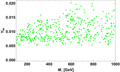
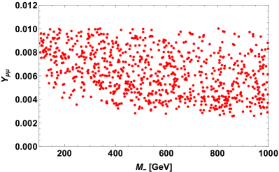
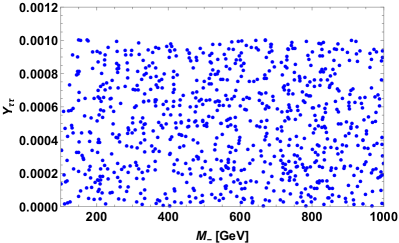
Figure 7: Allowed parameter space consistent with the current data from neutrino sector in $Y_{ll}-M_{-}$ plane.

VI Flavor Phenomenology

The general effective Hamiltonian responsible for the quark level transition $b\to sl^{+}l^{-}$ is given by Bobeth et al. (2000, 2002)

$${\cal H}_{\rm eff} = -\frac{4G_{F}}{\sqrt{2}}V_{tb}V_{ts}^{*}\Bigg{[}\sum_{i=1}^{6}C_{i}(\mu)O_{i}+\sum_{i=7,9,10}\Big{(}C_{i}(\mu)O_{i}+C_{i}^{\prime}(\mu)O_{i}^{\prime}\Big{)}\Bigg{]}\;,$$ (28)

where $G_{F}$ is the Fermi constant and $V_{qq^{\prime}}$ denote the Cabibbo-Kobayashi-Maskawa (CKM) matrix elements. The $C_{i}$’s stand for the Wilson coefficients evaluated at the renormalized scale $\mu=m_{b}$ Hou et al. (2014), where the sum over $i$ includes the current-current operators $(i=1,2)$ and the QCD-penguin operators $(i=3,4,5,6)$. The quark level operators mediating leptonic/semileptonic processes are given as

$$O_{7}^{(\prime)} = \frac{e}{16\pi^{2}}\Big{[}\bar{s}\sigma_{\mu\nu}\left(m_{s}P_{L(R)}+m_{b}P_{R(L)}\right)b\Big{]}F^{\mu\nu},$$

$$O_{9}^{(\prime)} = \frac{\alpha_{\rm em}}{4\pi}(\bar{s}\gamma^{\mu}P_{L(R)}b)(\bar{l}\gamma_{\mu}l)\;,~{}~{}~{}~{}~{}~{}~{}O_{10}^{(\prime)}=\frac{\alpha_{\rm em}}{4\pi}(\bar{s}\gamma^{\mu}P_{L(R)}b)(\bar{l}\gamma_{\mu}\gamma_{5}l)\;,$$ (29)

where $\alpha_{\rm em}$ denotes the fine-structure constant and $P_{L,R}=(1\mp\gamma_{5})/2$ are the chiral operators. The primed operators are absent in the SM, but can exist in the proposed $L_{\mu}-L_{\tau}$ model.

The previous section has discussed the available new parameter space consistent with the DM observables which are within their respective experimental limits. However, these parameters can be further constrained from the quark and lepton sectors, to be presented in the subsequent sections.

VI.1 $B_{s}-\bar{B}_{s}$ mixing

In this subsection, we discuss the constraint on the new parameters from the mass difference between the $B_{s}$ meson mass eigenstates ($\Delta M_{s}$), which characterizes the $B_{s}-\bar{B}_{s}$ mixing phenomena. In the SM, $B_{s}-\bar{B}_{s}$ mixing proceeds to an excellent approximation through the box diagram with internal top quark and $W$ boson exchange. The effective Hamiltonian describing the $\Delta B=2$ transition is given by Inami and Lim (1981)

$${\cal H}_{\rm eff}=\frac{G_{F}^{2}}{16\pi^{2}}~{}\lambda_{t}^{2}~{}M_{W}^{2}S_{0}(x_{t})\eta_{B}(\bar{s}b)_{V-A}(\bar{s}b)_{V-A}\;,$$ (30)

where $\lambda_{t}=V_{tb}V_{ts}^{*}$, $\eta_{B}$ is the QCD correction factor and the loop function $S_{0}(x_{t})$ is given by Inami and Lim (1981)

$$S_{0}(x_{t})=\frac{4x_{t}-11x_{t}^{2}+x_{t}^{3}}{4(1-x_{t})^{2}}-\frac{3}{2}\frac{\log x_{t}x_{t}^{3}}{(1-x_{t})^{3}}\;,$$ (31)

with $x_{t}=m_{t}^{2}/M_{W}^{2}$. Using Eqn. (30), the $B_{s}-\bar{B}_{s}$ mass difference in the SM is given as

$$\Delta M_{s}^{\rm SM}=2|M_{12}^{\rm SM}|=\frac{\langle\bar{B}_{s}|{\cal H}_{eff}|B_{s}\rangle}{M_{B_{s}}}=\frac{G_{F}^{2}}{6\pi^{2}}M_{W}^{2}~{}\lambda_{t}^{2}~{}\eta_{B}~{}\hat{B}_{s}f_{B_{s}}^{2}M_{B_{s}}S_{0}(x_{t})\;.$$ (32)

The SM predicted value of $\Delta M_{s}$ by using the input parameters from Tanabashi et al. (2018); Charles et al. (2015) is

$$\Delta M_{s}^{\rm SM}=(17.426\pm 1.057)~{}{\rm ps^{-1}},$$ (33)

and the corresponding experimental value is Tanabashi et al. (2018)

$$\Delta M_{s}^{\rm Expt}=17.761\pm 0.022~{}{\rm ps^{-1}}.$$ (34)

Even though the theoretical prediction is in good agreement with the experimental $B_{s}-\bar{B}_{s}$ oscillation data, it does not completely rule out the possibility of new physics.

Figure 8: Box diagrams of $B_{s}-\bar{B}_{s}$ mixing with leptoquark in the loop.

The box diagrams for $B_{s}-\bar{B}_{s}$ mixing in the presence of singlet SLQ and $N_{\pm}$ are shown in Fig. 8 . The effective Hamiltonian in the presence NP is given by

$${\cal H}_{\rm eff}=\frac{(y_{sR}y_{bR})^{2}}{128\pi^{2}M_{S_{1}}^{2}}\cos^{2}\alpha\sin^{2}\alpha C_{B_{s}}^{\rm NP}\left(\bar{s}b\right)_{V+A}\left(\bar{s}b\right)_{V+A}\;,$$ (35)

where

$$C_{B_{s}}^{\rm NP} = 2k\left(\chi_{-},\chi_{-},1\right)+4k\left(\chi_{-},\chi_{+},1\right)+2k\left(\chi_{+},\chi_{+},1\right)+\chi_{-}j\left(\chi_{-},\chi_{-},1\right)$$ (36)

$$+ 2\sqrt{\chi_{-}\chi_{+}}j\left(\chi_{-},\chi_{+},1\right)+\chi_{+}j\left(\chi_{+},\chi_{-},1\right),$$

with $\chi_{\mp}=M_{\mp}^{2}/M_{S_{1}}^{2}$ and the loop functions $k\left(\chi_{\pm},\chi_{\mp},1\right),~{}j\left(\chi_{\pm},\chi_{\mp},1\right)$ are given in Appendix A. Using Eqn. (35), the mass difference of $B_{s}-\bar{B}_{s}$ mixing due to the exchange of $S_{1}$ and $N_{\pm}$ is found to be

$$\Delta M_{s}^{\rm NP}=\frac{(y_{sR}y_{bR})^{2}}{48\pi^{2}M_{S_{1}}^{2}}\cos^{2}\alpha\sin^{2}\alpha C_{B_{s}}^{\rm NP}\eta_{B}\hat{B}_{B_{s}}f_{B_{s}}^{2}M_{B_{s}}\;.$$ (37)

Including the NP contribution arising due to the SLQ exchange, the total mass difference can be written as

$$\Delta M_{s}=\Delta M_{s}^{\rm SM}\left[1+\frac{C_{B_{s}}^{\rm NP}\cos^{2}\alpha\sin^{2}\alpha}{8G_{F}^{2}V_{tb}^{2}V_{ts}^{*2}M_{W}^{2}S_{0}(x_{t})}\left(\frac{(y_{sR}y_{bR})^{2}}{M_{S_{1}}^{2}}\right)\right]\;.$$ (38)

Using Eqns. (33) and (34) in (38), one can put bound on $(y_{qR})^{2}$ and $M_{-}$ parameters.

VI.2 $B\to Kl^{+}l^{-}$ process

The rare semileptonic $B\to Kl^{+}l^{-}$ process is mediated via $b\to sl^{+}l^{-}$ quark level transitions. In the current framework, the $b\to sl^{+}l^{-}$ transitions can occur via the $Z^{\prime}$ exchanging one-loop penguin diagrams shown in Fig. 9 .

Figure 9: Penguin diagram of $b\to sll$ processes, where $\l=\mu,\tau$ with leptoquark in the loop.

The penguin diagram in the left panel is suppressed by the factor, $m_{b}/M_{\pm}$, thus providing negligible contribution. Furthermore, due to the zero hypercharge of dark matter fermion, the diagrams with SM neutral bosons ($Z,\gamma$) replacing $Z^{\prime}$ in the right panel of Fig. 9  are not possible in the present framework. The matrix elements of the various hadronic currents between the initial $B$ meson and $K$ meson in the final state are related to the form factors $f_{+,0}$ as follows Bobeth et al. (2007); Ball and Zwicky (2005)

$$\langle{K}\left(p_{K}\right)|\bar{s}\gamma^{\mu}b|{B}\left(p_{B}\right)\rangle=f_{+}\left(q^{2}\right)\left(p_{B}+p_{K}\right)^{\mu}+\left[f_{0}\left(q^{2}\right)-f_{+}\left(q^{2}\right)\right]\frac{M^{2}_{B}-M^{2}_{K}}{q^{2}}q^{\mu}\,,$$ (39)

where $p_{B}~{}(p_{K})$ and $M_{B}~{}(M_{K})$ denote the 4-momenta and mass of the $B~{}(K)$ meson and $q^{2}$ is the momentum transfer. By using Eqn. (39), the transition amplitude of $B\to K\mu^{+}\mu^{-}$ process is given by

$$\mathcal{M}=\frac{1}{2^{5}\pi^{2}}\frac{y_{bR}y_{sR}g_{\mu\tau}^{2}}{M_{Z^{\prime}}^{2}}\mathcal{V}_{sb}(\chi_{-},\chi_{+})[\bar{u}(p_{B})\gamma^{\mu}(1+\gamma_{5})u(p_{K}))][\bar{v}(p_{2})\gamma_{\mu}u(p_{1}))],$$ (40)

where $p_{1}$ and $p_{2}$ are the four momenta of charged leptons and the loop function $\mathcal{V}_{sb}(\chi_{-},\chi_{+})$ is given in Appendix A Baek (2018); Hisano et al. (1996). Now comparing this amplitude (40) with the amplitude obtained from the effective Hamiltonian (28), we obtain a new Wilson coefficient associated with the right-handed semileptonic electroweak penguin operator $\mathcal{O}_{9}^{\prime}$ as

$$C_{9}^{\prime\rm NP}=\frac{\sqrt{2}}{2^{4}\pi G_{F}\alpha_{\rm em}V_{tb}V_{ts}^{*}}\frac{y_{bR}y_{sR}g_{\mu\tau}^{2}}{{M_{Z^{\prime}}}^{2}}\mathcal{V}_{sb}\left(\chi_{-},\chi_{+}\right)\,.$$ (41)

The differential branching ratio of $B\to Kll$ process with respect to $q^{2}$ is given by

$$\frac{d{\rm Br}}{dq^{2}}=\tau_{B}\frac{G_{F}^{2}\alpha_{\rm em}^{2}|V_{tb}V_{ts}^{*}|^{2}}{2^{8}\pi^{5}M_{B}^{3}}\sqrt{\lambda(M_{B}^{2},M_{K}^{2},q^{2})}\beta_{l}f_{+}^{2}\Big{(}a_{l}(q^{2})+\frac{c_{l}(q^{2})}{3}\Big{)}\;,$$ (42)

where

$$a_{l}(q^{2}) = q^{2}|F_{P}|^{2}+\frac{\lambda(M_{B}^{2},M_{K}^{2},q^{2})}{4}(|F_{A}|^{2}+|F_{V}|^{2})$$

$$+2m_{l}(M_{B}^{2}-M_{K}^{2}+q^{2}){\rm Re}(F_{P}F_{A}^{*})+4m_{l}^{2}M_{B}^{2}|F_{A}|^{2}\;,$$

$$c_{l}(q^{2}) = -\frac{\lambda(M_{B}^{2},M_{K}^{2},q^{2})}{4}\beta_{l}^{2}\left(|F_{A}|^{2}+|F_{V}|^{2}\right),$$ (43)

with

$$F_{V} = \frac{2m_{b}}{M_{B}}C_{7}^{\rm eff}+C_{9}^{\rm eff}+C_{9}^{\prime\rm NP},~{}~{}~{}~{}~{}F_{A}=C_{10},$$

$$F_{P} = m_{l}C_{10}\Big{[}\frac{M_{B}^{2}-M_{K}^{2}}{q^{2}}\Big{(}\frac{f_{0}(q^{2})}{f_{+}(q^{2})}-1\Big{)}-1\Big{]}\;,$$ (44)

and

$$\lambda(a,b,c)=a^{2}+b^{2}+c^{2}-2(ab+bc+ca),~{}~{}~{}~{}~{}\beta_{l}=\sqrt{1-4m_{l}^{2}/q^{2}}\;.$$ (45)

For numerical estimation, we have used the lifetime and masses of particles from Tanabashi et al. (2018) and the form factors are taken from Colangelo et al. (1997). The experimental limit on the branching ratios of $\bar{B}^{0}\to\bar{K}^{0}\mu^{+}\mu^{-}$ and $B^{+}\to K^{+}\tau^{+}\tau^{-}$ processes are Tanabashi et al. (2018)

$${\rm Br}(\bar{B}^{0}\to\bar{K}^{0}\mu^{+}\mu^{-})\big{|}^{\rm Expt}=(3.39\pm 0.34)\times 10^{-7}\,,$$ (46)

$${\rm Br}(B^{+}\to K^{+}\tau^{+}\tau^{-})\big{|}^{\rm Expt}<2.5\times 10^{-3},$$ (47)

while their predicted values in the SM are

$${\rm Br}(\bar{B}^{0}\to\bar{K}^{0}\mu^{+}\mu^{-})\big{|}^{\rm SM}=(1.82\pm 0.15)\times 10^{-7}\,,$$ (48)

$${\rm Br}(B^{+}\to K^{+}\tau^{+}\tau^{-})\big{|}^{\rm SM}=(1.56\pm 0.125)\times 10^{-7}.$$ (49)

Since $Z^{\prime}$ doesn’t couple to electron, the branching ratio of $B\to Ke^{+}e^{-}$ process is considered to be SM like. The decay modes $\bar{B}^{0}\to\bar{K}^{0}\mu^{+}\mu^{-}$ and $B^{+}\to K^{+}\tau^{+}\tau^{-}$ can put constraint on all the four parameters, i.e., $(y_{qR})^{2},~{}g_{\mu\tau},~{}M_{Z^{\prime}}$ and $M_{-}$.

VI.3 $B\to X_{s}\gamma$ process

The $B\to X_{s}\gamma$ process involves $b\to s\gamma$ quark level transition, the experimental limit on the corresponding branching ratio is given by Amhis et al. (2017)

$${\rm Br}(B\to X_{s}\gamma)\big{|}^{\rm Expt}_{E_{\gamma}>1.6~{}{\rm GeV}}=(3.32\pm 0.16)\times 10^{-4}.$$ (50)

Fig. 10 represents the one loop penguin diagram of $b\to s\gamma$ process mediated by SLQ and $N_{\pm}$.

Figure 10: Feynman diagram of $b\to s\gamma$ processes in the presence of scalar leptoquark.

Including the NP contribution, the total branching ratio of $B\to X_{s}\gamma$ is given by

$${\rm Br}(B\to X_{s}\gamma)={\rm Br}(B\to X_{s}\gamma)\big{|}^{\rm SM}\Bigg{(}1+\frac{C_{7}^{\gamma\prime\rm NP}}{C_{7}^{\gamma\rm SM}}\Bigg{)}^{2},$$ (51)

where the predicted SM branching ratio is Misiak et al. (2015)

$${\rm Br}(B\to X_{s}\gamma)\big{|}^{\rm SM}_{E_{\gamma}>1.6~{}{\rm GeV}}=(3.36\pm 0.23)\times 10^{-4}.$$ (52)

The new $C_{7}^{\gamma\prime\rm NP}$ Wilson coefficient obtained from Fig. 10 is given by

$$C_{7}^{\gamma\prime\rm NP}=-\frac{\sqrt{2}/3}{8G_{F}V_{tb}V_{ts}^{*}}\frac{y_{bR}y_{sR}}{M_{S_{1}}^{2}}\Big{(}J_{1}(\chi_{-})\cos^{2}\alpha+J_{1}(\chi_{+})\sin^{2}\alpha\Big{)},$$ (53)

where the loop functions $J_{1}(\chi_{\pm})$ are given as Baek (2018)

$$J_{1}(\chi_{\pm})=\frac{1-6\chi_{\pm}+3\chi_{\pm}^{2}+2\chi_{\pm}^{3}-6\chi_{\pm}^{2}\log\chi_{\pm}}{12(1-\chi_{\pm})^{4}}\,.$$ (54)

Using Eqns. (50 , 52 , 53) in (51), the parameters $(y_{qR})^{2}$ and $M_{-}$ can be constrained.

VI.4 $\tau\to\mu\nu_{\tau}\bar{\nu}_{\mu}$ process

In the presence of $Z^{\prime}$ boson, the $\tau\to\mu\nu_{\tau}\bar{\nu}_{\mu}$ process can occur via box diagram as shown in Fig. 11 . There are four possible one-loop box diagrams with the $Z^{\prime}$ connected to the lepton legs.

Figure 11: One loop box diagram of $\tau\to\mu\nu_{\tau}\bar{\nu}_{\mu}$ processes.

The total branching ratio of this process is given by Altmannshofer et al. (2014a)

$${\rm Br}(\tau\to\mu\nu_{\tau}\bar{\nu}_{\mu})={\rm Br}(\tau\to\mu\nu_{\tau}\bar{\nu}_{\mu})\big{|}^{\rm SM}\Bigg{(}1+\frac{3g_{\mu\tau}^{2}}{4\pi^{2}}\frac{\log(M_{W}^{2}/M_{Z^{\prime}}^{2})}{1-M_{Z^{\prime}}^{2}/M_{W}^{2}}\Bigg{)}^{2},$$ (55)

where the branching ratio in the SM is given by Altmannshofer et al. (2014a)

$${\rm Br}(\tau\to\mu\nu_{\tau}\bar{\nu}_{\mu})\big{|}^{\rm SM}=(17.29\pm 0.032)\%.$$ (56)

Now comparing the theoretical result with the experimental measured value Tanabashi et al. (2018)

$${\rm Br}(\tau\to\mu\nu_{\tau}\bar{\nu}_{\mu})\big{|}^{\rm Expt}=(17.39\pm 0.04)\%,$$ (57)

one can put bounds on $M_{Z^{\prime}}-g_{\mu\tau}$ parameter space.

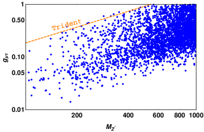
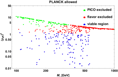
Figure 12: Left panel projects the constraint on $g_{\mu\tau}$ and $M_{Z^{\prime}}$ obtained from ${\rm Br}(B^{+}\to K^{+}\tau^{+}\tau^{-})$, ${\rm Br}(\bar{B}^{0}\to\bar{K}^{0}\mu^{+}\mu^{-})$ and ${\rm Br}(\tau\to\mu\nu_{\tau}\bar{\nu}_{\mu})$ observables. Dashed orange line denotes the neutrino trident bound Mishra et al. (1991); Altmannshofer et al. (2014b). In the right panel, blue data points denote the allowed parameter space obtained from ${\rm Br}(\bar{B}^{0}\to\bar{K}^{0}\mu^{+}\mu^{-})$, $B_{s}-\bar{B_{s}}$ mixing, ${\rm Br}(B^{+}\to K^{+}\tau^{+}\tau^{-})$, Br($B\to X_{s}\gamma)$ experimental data, which are also consistent with Planck (Aghanim et al., 2018) and PICO-60 limit Amole et al. (2017). Here, green (red) data points denote PICO-60 and flavor excluded (PICO-60 allowed and flavor excluded) region.

Parameters	DM-I	DM-II	DM+Flavor
$M_{-}$ [GeV]	$103-560$	$561-988$	$103-560$
$(y_{qR})^{2}$	$0-3.51$	$1.94-2.56$	$0-1.26$

Table 2: Predicted allowed range of parameters $M_{-}$ and $(y_{qR})^{2}$. Here DM-I and DM-II represent two regions in Fig. 4 consistent with only DM observables, DM+Flavor denotes the region favored by both the dark matter and flavor studies.

Now correlating the theoretical predictions of ${\rm Br}(\bar{B}^{0}\to\bar{K}^{0}\mu^{+}\mu^{-})$, ${\rm Br}(B^{+}\to K^{+}\tau^{+}\tau^{-})$ and ${\rm Br}(\tau\to\mu\nu_{\tau}\bar{\nu}_{\mu})$ with the corresponding $3\sigma$ experimental data, we compute the $M_{Z^{\prime}}-g_{\mu\tau}$ allowed parameter space. Since $Z^{\prime}$ does not couple to quarks, these gauge parameters couldn’t be constrained from $b\to s\gamma$ decay modes and $B_{s}-\bar{B}_{s}$ oscillation data. The constraint on $M_{-}-(y_{qR})^{2}$ parameter space is obtained from ${\rm Br}(\bar{B}^{0}\to\bar{K}^{0}\mu^{+}\mu^{-})$, ${\rm Br}(B^{+}\to K^{+}\tau^{+}\tau^{-})$, ${\rm Br}(B\to X_{s}\gamma)$ and $B_{s}-\bar{B}_{s}$ mixing results. In addition, the branching ratio of rare semileptonic $B\to K\nu_{l}\bar{\nu}_{l}$ process can play a vital role in restricting these parameters. Though the proposed model can allow $b\to s\nu_{l}\bar{\nu}_{l}$ decay modes, but the contributions of $\mu$ and $\tau$ leptons cancel with each other in the leading order of NP due to their equal and opposite $L_{\mu}-L_{\tau}$ charges. Since there is no $Z^{\prime}\mu\tau$ coupling, the neutral and charged lepton flavor violating decay processes like $B\to K^{(*)}\mu^{\mp}\tau^{\pm}$, $\tau^{-}\to\mu^{-}\gamma$, $\tau\to\mu\mu\mu$ do not play any role. It should be noted that, the model considered here provides only additional contribution to $b\to sll$ transitions through $C_{9}^{\prime{\rm NP}}$ coefficient, hence the $B_{s}\to l^{+}l^{-}$ processes could not provide any strict bound on the new parameters. In this analysis, we consider that the $y_{qR}$ coupling is perturbative, i.e., $|y_{qR}|\lesssim\sqrt{4\pi}$. Left (right) panel in Fig. 12 denotes the parameter space in the plane of $M_{Z^{\prime}}-g_{\mu\tau}$ ($M_{-}-(y_{qR})^{2}$) consistent with DM and flavor studies. From left panel, one can see that the obtained parameter space survives the lower limit imposed on the ratio $M_{Z^{\prime}}/g_{\mu\tau}$ by neutrino trident production Mishra et al. (1991); Altmannshofer et al. (2014b), i.e., $540$ GeV. It is also noted that the allowed region favored by the $(g-2)_{\mu}$ anomaly is completely excluded by the constraint from the neutrino trident production Altmannshofer et al. (2014a). In the right panel of Fig. 12 , we redisplay $M_{-}-(y_{qR})^{2}$ parameter space of Fig. 4 after a combined analysis made by imposing the DM and flavor experimental limits, with the surviving region shown in blue color. In Table 2, we report the allowed region of the parameters $M_{-}$ and $(y_{qR})^{2}$ which are consistent with only DM studies (DM-I,II), both DM and flavor sectors (DM+Flavor).

To illustrate the relative contribution of annihilation channels to relic density for the parameter space depicted in Fig. 12, we choose two benchmark values (Table. 3), particularly the composition of maximum $(y_{qR})^{2}$ and minimum $g_{\mu\tau}$ (benchmark-1) and vice-versa (benchmark-2). For these values, we show the relative contribution of each $S_{1}$-portal ($Z^{\prime}$-portal) channel in the left (right) panel of Fig. 13. For benchmark-1 i.e., maximal $(y_{qR})^{2}$, the contribution (blue curve) from SLQ-portal channels - $d\bar{d},s\bar{s},b\bar{b}$ ($\sim 32\%$ each) dominate over $(Z^{\prime},H_{1,2},\eta)$-portal contribution (green curve) for almost whole DM mass region except near the resonances in propagators $Z^{\prime},H_{1}$ and $H_{2}$. Similarly, for benchmark-2 i.e., maximal $g_{\mu\tau}$, the $Z^{\prime}$-portal channels - $\mu\bar{\mu},\tau\bar{\tau},\nu_{\mu}\bar{\nu}_{\mu},\nu_{\tau}\bar{\nu}_{\tau}$ ($\sim 24\%$ each) provide dominant contribution (blue curve) over the rest (green curve) with exception to the region near resonances of the propagators $H_{1}$ and $H_{2}$. The contribution of the channel with $Z^{\prime}H_{1}$ in the final state is negligible due to $\zeta^{2}$ (Higgs mixing) factor, the process with $Z^{\prime}H_{2}$ as final state particles is not kinematically allowed ($M_{H_{2}}=2.4$ TeV) for the displayed DM mass range. In the rest of the parameter region of Fig. 12, the dominant contribution however, depends on all the four parameters listed in Table. 3.

S.No	$(y_{qR})^{2}$	$g_{\mu\tau}$	$M_{Z^{\prime}}$ [GeV]	$M_{-}$ [GeV]
1.	$1.016$	$0.336$	$669.84$	$291.22$
2.	$0.0003$	$0.94$	$763.29$	$496.7$

Table 3: Sample benchmark values chosen from the allowed paramter space of Fig. 12.

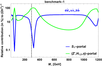
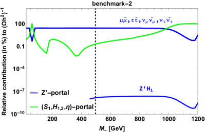
Figure 13: Left and right panels depict the relative contribution of annihilation channels for the benchmark values of Table. 3. Vertical dashed line represents value of DM mass corresponding to the benchmark.

VII Implication on $R_{K}$ and $B_{(s)}\to K^{*}(\phi)\mu^{+}\mu^{-}$ Processes

The constrained parameter space discussed in the previous section can have an impact on $R_{K}$ and the observables of $B\to Vl^{+}l^{-}$ process, where $V=K^{*},\phi$ are the vector mesons, which subsequently decay into $K^{*}\to K\pi$ and $\phi\to K^{+}K^{-}$ states. The $B\to V$ hadronic matrix elements of the local quark bilinear operators can be parametrized as Ali et al. (2000); Wirbel et al. (1985)

$$\langle V\left(k\right)|\bar{s}\gamma_{\mu}(1-\gamma_{5})b|B\left(p\right)\rangle=\epsilon_{\mu\nu\alpha\beta}\epsilon^{*\nu}p^{\alpha}q^{\beta}\frac{2V(q^{2})}{M_{B}+M_{V}}-i\epsilon^{*}_{\mu}(M_{B}+M_{V})A_{1}(q^{2})$$

$$\hskip 56.9055pt+i(\epsilon^{*}\cdotp q)(2p-q)_{\mu}\frac{A_{2}(q^{2})}{M_{B}+M_{V}}+i\frac{2M_{V}}{q^{2}}(\epsilon^{*}\cdotp q)\left[A_{3}(q^{2})-A_{0}(q^{2})\right]q_{\mu}\;,$$ (58)

where

$$A_{3}(s)=\frac{(M_{B}+M_{V})}{2M_{V}}A_{1}(s)-\frac{(M_{B}-M_{V})}{2M_{V}}A_{2}(s),$$ (59)

$q^{2}$ is the momentum transfer between the $B$ and $V$ mesons, i.e., $q_{\mu}=p_{\mu}-k_{\mu}$ and $\epsilon_{\mu}$ is the polarization vector of the $V$ meson. The full angular differential decay distribution for the processes $B^{0}\to(K^{*0}\to K^{-}\pi^{+})l^{+}l^{-}$ and $B_{s}\to(\phi\to K^{+}K^{-})l^{+}l^{-}$ in terms of $q^{2}$, $\theta_{l}$, $\theta_{V}$ and $\phi$ variables is given as Bobeth et al. (2008); Egede et al. (2010, 2008)

$$\frac{d^{4}\Gamma}{dq^{2}~{}d\cos\theta_{l}~{}d\cos\theta_{V}~{}d\phi}=\frac{9}{32\pi}J\left(q^{2},\theta_{l},\theta_{V},\phi\right)\;,$$ (60)

where

$$J\left(q^{2},\theta_{l},\theta_{V},\phi\right) = J^{s}_{1}\sin^{2}\theta_{V}+J^{c}_{1}\cos^{2}\theta_{V}+\left(J^{s}_{2}\sin^{2}\theta_{V}+J^{c}_{2}\cos^{2}\theta_{V}\right)\cos 2\theta_{l}$$ (61)

$$+ J_{3}\sin^{2}\theta_{V}\sin^{2}\theta_{l}\cos 2\phi+J_{4}\sin 2\theta_{V}\sin 2\theta_{l}\cos\phi+J_{5}\sin 2\theta_{V}\sin\theta_{l}\cos\phi$$

$$+ (J_{6}^{s}\sin^{2}\theta_{V}+J_{6}^{c}\cos^{2}\theta_{V})\cos\theta_{l}+J_{7}\sin 2\theta_{V}\sin\theta_{l}\sin\phi$$

$$+ J_{8}\sin 2\theta_{V}\sin 2\theta_{l}\sin\phi+J_{9}\sin^{2}\theta_{V}\sin^{2}\theta_{l}\sin 2\phi\;,$$

$\theta_{l}$ is the angle between $l^{-}$ and $B_{(s)}$ in the dilepton frame, $\theta_{V}$ is defined as the angle between $K^{-}$ and $B_{(s)}$ in the $K^{-}\pi^{+}~{}(K^{-}K^{+})$ frame, the angle between the normal of the $K^{-}\pi^{+}~{}(K^{-}K^{+})$ and the dilepton planes is given by $\phi$. The complete expressions for $J_{i}^{s(c)},~{}i=1,2,...,9$ as a function of transversity amplitudes are given in the Appendix B Altmannshofer et al. (2009). The transversity amplitudes written in terms of the form factors and Wilson coefficients are as follows Altmannshofer et al. (2009)

$$A_{\perp L,R} = N\sqrt{2\lambda}\Big{[}\left((C_{9}^{\rm eff}+C_{9}^{\prime\rm NP})\mp C_{10}\right)\frac{V(q^{2})}{M_{B}+M_{V}}+\frac{2m_{b}}{q^{2}}C_{7}T_{1}(q^{2})\Big{]}\;,$$

$$A_{\parallel L,R} = -N\sqrt{2}(M_{B}^{2}-M_{V}^{2})\Big{[}\left((C_{9}^{\rm eff}-C_{9}^{\prime\rm NP})\mp C_{10}\right)\frac{A_{1}(q^{2})}{M_{B}-M_{V}}+\frac{2m_{b}}{q^{2}}C_{7}T_{2}(q^{2})\Big{]}\;,$$

$$A_{0L,R} = -\frac{N}{2M_{V}\sqrt{s}}\Big{[}\left(C_{9}^{\rm eff}-C_{9}^{\prime\rm NP})\mp C_{10}\right)$$

$$\times\left((M_{B}^{2}-M_{V}^{2}-q^{2})(M_{B}+M_{V})A_{1}(q^{2})-\lambda\frac{A_{2}(q^{2})}{M_{B}+M_{V}}\right)$$

$$+2m_{B}C_{7}\left((M_{B}^{2}+3M_{V}^{2}-q^{2})T_{2}(q^{2})-\frac{\lambda}{M_{B}^{2}-M_{V}^{2}}\right)\Big{]}\;,$$

$$A_{t} = 2N\sqrt{\frac{\lambda}{q^{2}}}C_{10}A_{0}(q^{2}),$$ (62)

where

$$N=V_{tb}V_{ts}^{*}\left[\frac{G_{F}^{2}\alpha_{\rm em}^{2}}{3\cdot 2^{10}\pi^{5}M_{B}^{3}}q^{2}\beta_{l}\sqrt{\lambda}\right]^{1/2}\;,~{}~{}~{}~{}~{}~{}\lambda=\lambda(M_{V}^{2},M_{B}^{2},q^{2}).$$ (63)

The dilepton invariant mass spectrum for ${B}\rightarrow Vl^{+}l^{-}$ decay after integration over all angles Bobeth et al. (2008) is given by

$$\frac{d\Gamma}{dq^{2}}=\frac{3}{4}\left(J_{1}-\frac{J_{2}}{3}\right),$$ (64)

where $J_{i}=2J_{i}^{s}+J_{i}^{c}$. The most interesting observables in these decay modes are the lepton non-universality parameter defined as

$$R_{V}=\frac{{\rm Br}(B\to V\mu^{+}\mu^{-})}{{\rm Br}(B\to Ve^{+}e^{-})},$$ (65)

and the form factor independent (FFI) observables Descotes-Genon et al. (2013)

$$P_{4}^{\prime}=\frac{J_{4}}{\sqrt{-J_{2}^{s}J_{2}^{c}}},~{}~{}~{}~{}~{}P_{5}^{\prime}=\frac{J_{5}}{2\sqrt{-J_{2}^{s}J_{2}^{c}}}.$$ (66)

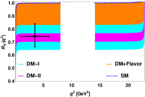
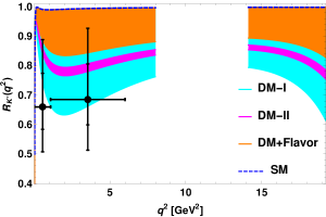
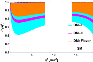
Figure 14: The $q^{2}$ variation of $R_{K}$ (top-left panel), $R_{K^{*}}$ (top-right panel) and $R_{\phi}$ (bottom panel) LNU parameters in the $L_{\mu}-L_{\tau}$ model. Here the blue dashed lines represent the SM prediction, the cyan (magenta) bands stand for the NP contribution from the dark matter studies i.e., DM-I (DM-II). Orange bands are due to the contribution from both the flavor and DM sectors (DM+Flavor). The experimental data points (with 2$\sigma$ error bars) Aaij et al. (2017) are shown in black lines .

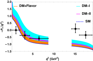
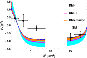
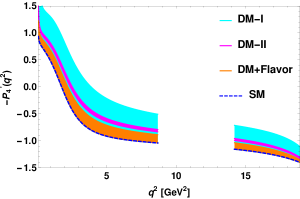
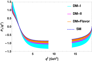
Figure 15: Top panel represents the variation of $P_{4}^{\prime}$ (left panel) and $P_{5}^{\prime}$ (right panel) observables of $B^{0}\to K^{*0}\mu^{+}\mu^{-}$ process with respect to $q^{2}$. The behaviour of $P_{4}^{\prime}$ (left panel) and $P_{5}^{\prime}$ (right panel) for $B_{s}\to\phi\mu^{+}\mu^{-}$ are shown in the bottom panel. The bin-wise experimental data points with error bars are shown in black Aaij et al. (2013b). Note that $P_{4}^{\prime}\big{|}^{\rm LHCb}=-P_{4}^{\prime}$.

After getting familiar with the different observables and the allowed values of the new parameters, we now proceed for numerical analysis in the full dilepton mass region i.e., $4m^{2}_{l}\leqslant q^{2}\leqslant\left(M_{B}-M_{V}\right)^{2}$, leaving the regions around $q^{2}\sim m_{J/\psi}^{2}$ and $m_{\psi^{\prime}}^{2}$. The cuts are employed to remove the dominant charmonium resonance $\left(c\bar{c}\right)=J/\psi,\psi^{\prime}$ backgrounds from $B\rightarrow V\left(c\bar{c}\right)\rightarrow Vl^{+}l^{-}$. In Fig. 14 , we show the behaviour of $R_{K}$ (top-left panel), $R_{K^{*}}$ (top-right panel) and $R_{\phi}$ (bottom panel) with respect to $q^{2}$ in the full kinematically accessible physical region. In these figures, the blue dashed lines stand for the SM contribution, the orange bands are due to the allowed region of parameters shown in Table 2 , favored by both DM and flavor (DM+Flavor) and cyan (magenta) bands for only DM case i.e., DM-I (DM-II). The bin-wise experimental values of $R_{K^{(*)}}$ are shown in black. From the top-left panel of Fig. 14 , it can be seen that the result obtained in the $q^{2}\in[1,6]~{}{\rm GeV}^{2}$ bin, by using the constraint from only DM observable is consistent with the experimental data and can be explained within $1\sigma$ for DM+Flavor case. The measured value of $R_{K^{*}}$ in the $q^{2}\in[0.045,1.1]~{}{\rm GeV}^{2}$ bin can be accommodated within $1\sigma$ (DM-I) and $2\sigma$ (DM-II and DM+Flavor), $q^{2}\in[1.1,6]~{}{\rm GeV}^{2}$ bin result can be described within $1\sigma$ (DM-II) and $2\sigma$ (DM+Flavor) and is consistent with experimental data for DM-I case. Though there is no experimental evidence for $R_{\phi}$ parameter, the additional NP contribution arising from the allowed parameter space of all cases (DM-I,II and DM+Flavor) provide significant deviation from the SM prediction, implying the presence of lepton universality violation in the $B_{s}\to\phi\mu^{+}\mu^{-}$ process. In Table 4 , we present our predicted values of $R_{K^{(*)}}$ and $R_{\phi}$ for different bins. The $q^{2}$ variation of famous optimized observables $-P_{4}^{\prime}$ (top-left panel) and $P_{5}^{\prime}$ (top-right panel) of $B^{0}\to K^{*0}\mu^{+}\mu^{-}$ process are depicted in Fig. 15 . The bottom panel of this figure describes analogous plots for $B_{s}\to\phi\mu^{+}\mu^{-}$ process in both the high and low recoil limit. It should be noted that $P_{4}^{\prime}\big{|}^{\rm LHCb}=-P_{4}^{\prime}$. In the low $q^{2}$ region, our predictions on $-P_{4}^{\prime}$ observable of $B^{0}\to K^{*0}\mu^{+}\mu^{-}$ process is in very good agreement with the LHCb data. For $B^{0}\to K^{*0}\mu^{+}\mu^{-}$ decay mode, the model can accommodate the $P_{5}^{\prime}$ observable within $1\sigma$ range of the experimental data, in the high and very low $q^{2}$ region. We notice considerable deviation between the results of SM and the presented $L_{\mu}-L_{\tau}$ model on the $P_{4,5}^{\prime}$ observables for $B_{s}\to\phi\mu^{+}\mu^{-}$ decay modes. The numerical values of all these observables are given in Table 4 . We found that our results on the angular observables of $B\to Vll$ process, obtained from DM-I parameter space are almost consistent with the corresponding measured experimental data.

	Observables	Values for SM	Values for DM-I	Values for DM-II	Values for DM+Flavor
	$R_{K^{*}}|_{q^{2}\in[0.045,1.1]~{}{\rm GeV}^{2}}$	$0.949$	$0.793-0.949$	$0.852-0.863$	$0.881-0.949$
$B^{0}$	$R_{K^{*}}|_{q^{2}\in[1.1,6]~{}{\rm GeV}^{2}}$	$0.993$	$0.671-0.993$	$0.786-0.811$	$0.848-0.993$
$\downarrow$	$R_{K^{*}}|_{q^{2}\geq 14.18~{}{\rm GeV}^{2}}$	$0.998$	$0.754-0.998$	$0.832-0.851$	$0.879-0.998$
$K^{*0}$	$P_{5}^{\prime}|_{q^{2}\in[1,6]~{}{\rm GeV}^{2}}$	$-0.542\pm 0.044$	$-0.82\to-0.542$	$-0.655\to-0.635$	$-0.612\to-0.542$
$\mu^{+}$	$P_{5}^{\prime}|_{q^{2}\geq 14.18~{}{\rm GeV}^{2}}$	$-0.695\pm 0.056$	$-1.165\to-0.695$	$-0.894\to-0.86$	$-0.818\to-0.695$
$\mu^{-}$	$P_{4}^{\prime}|_{q^{2}\in[1,6]~{}{\rm GeV}^{2}}$	$0.563\pm 0.045$	$-0.239\to 0.563$	$0.195-0.257$	$0.334\to 0.563$
	$P_{4}^{\prime}|_{q^{2}\geq 14.18~{}{\rm GeV}^{2}}$	$1.2\pm 0.096$	$0.787-1.2$	$1.03-1.06$	$1.098-1.2$
	$R_{\phi}|_{q^{2}\in[0.045,1.1]~{}{\rm GeV}^{2}}$	$0.9499$	$0.753-0.9499$	$0.828-0.844$	$0.866-0.9499$
$B_{s}$	$R_{\phi}|_{q^{2}\in[1.1,6]~{}{\rm GeV}^{2}}$	$0.994$	$0.642-0.994$	$0.77-0.8$	$0.839-0.994$
$\downarrow$	$R_{\phi}|_{q^{2}\geq 14.18~{}{\rm GeV}^{2}}$	$0.998$	$0.731-0.998$	$0.82-0.84$	$0.871-0.998$
$\phi$	$P_{5}^{\prime}|_{q^{2}\in[1,6]~{}{\rm GeV}^{2}}$	$-0.511\pm 0.041$	$-0.766\to-0.551$	$-0.618\to-0.599$	$-0.578\to-0.511$
$\mu^{+}$	$P_{5}^{\prime}|_{q^{2}\geq 14.18~{}{\rm GeV}^{2}}$	$-0.645\pm 0.052$	$-1.1\to-0.645$	$-0.839\to-0.805$	$-0.765\to-0.645$
$\mu^{-}$	$P_{4}^{\prime}|_{q^{2}\in[1,6]~{}{\rm GeV}^{2}}$	$0.596\pm 0.048$	$-0.202\to 0.596$	$0.228-0.29$	$0.367\to 0.596$
	$P_{4}^{\prime}|_{q^{2}\geq 14.18~{}{\rm GeV}^{2}}$	$1.233\pm 0.099$	$0.822-1.233$	$1.059-1.092$	$1.13-1.233$
	$R_{K}|_{q^{2}\in[1,6]~{}{\rm GeV}^{2}}$	$1.0004$	$0.643-1.0004$	$0.71-0.766$	$0.834-1.0004$
	$R_{K}|_{q^{2}\geq 14.18~{}{\rm GeV}^{2}}$	$1.002$	$0.645-1.002$	$0.71-0.768$	$0.836-1.002$

Table 4: Predicted numerical values of LNU parameters $(R_{V})$ and $P_{4,5}^{\prime}$ observables of $B_{(s)}\to V\mu^{+}\mu^{-},~{}V=K^{*},\phi$ processes in the high and low recoil limits. The values of $R_{K}$ parameter are also presented in both low and high $q^{2}$ regime

.

VIII Summary and Conclusion

Summarizing the article, we have studied Majorana dark matter in a new version of $U(1)_{L_{\mu}-L_{\tau}}$ gauge extension of the standard model. The model is free from triangle gauge anomalies with the inclusion of three neutral fermions with $L_{\mu}-L_{\tau}$ charges $0,1$ and $-1$. A scalar singlet, charged $+2$ under the new $U(1)$ is added to spontaneously break the $L_{\mu}-L_{\tau}$ gauge symmetry, thereby giving masses to the new fermions and the neutral boson $Z^{\prime}$ associated with gauge extension. In addition, the scalar sector is enriched with an inert doublet and a $(\bar{3},1,1/3)$ scalar leptoquark to obtain the neutrino mass at one-loop level and address the flavor anomalies respectively. All the new fermions, leptoquark and inert doublet are assigned with charge $-1$ under $Z_{2}$ symmetry. Choosing the lightest mass eigenstate of the new fermion spectrum as dark matter, we made a thorough study of Majorana dark matter in relic density and direct detection perspective. The channels contributing to relic density are mediated by the scalar leptoquark, $Z^{\prime}$ and inert doublet components. As $Z^{\prime}$ doesn’t couple to quarks, the $Z^{\prime}$-mediated tree level interaction for direct detection is not permitted. Only leptoquark portal channels contribute to spin-dependent WIMP-nucleon cross section. Imposing Planck limit on relic density and well known PICO-60, LUX bounds on spin-dependent cross section, we have constrained the new parameters of the model. We have also computed the spin-dependent and spin-independent contributions of one-loop diagrams involving scalar leptoquark, but found to give zero impact on the model parameters. We have also showed the mechanism of generating light neutrino mass radiatively using the inert doublet. A note on the viable parameter region consistent with neutrino oscillation data is also addressed.

We have further restricted the new parameters from quark and lepton sectors i.e., by comparing the theoretical predictions of ${\rm Br}(\tau\to\mu\nu_{\tau}\bar{\nu}_{\mu})$, ${\rm Br}(B\to X_{s}\gamma)$, ${\rm Br}(B^{+}\to K^{+}\tau^{+}\tau^{-})$, ${\rm Br}(\bar{B}^{0}\to\bar{K}^{0}\mu^{+}\mu^{-})$ and $B_{s}-\bar{B}_{s}$ mixing with their corresponding $3\sigma$ experimental data. The neutral and charged lepton flavor violating decay processes are absent due to zero $Z^{\prime}\tau\mu$ coupling. And also the vanishing $Z^{\prime}q\bar{q}$ coupling restricts the involvement of $Z^{\prime}$ in $B_{s}-\bar{B}_{s}$ mixing, $b\to s\gamma$ processes at one-loop level. We have then investigated the implication on $P^{\prime}_{4,5}$, $R_{K^{(*)}}$ and $R_{\phi}$ observables of $B_{(s)}\to K^{(*)}(\phi)l^{+}l^{-}$ decay modes in the full kinematically allowed $q^{2}$ region for two cases i.e., dark matter and flavor allowed, only dark matter allowed parameter space. We observed that our model can explain the $R_{K}$ LNU parameter very well. The $R_{K^{*}}$ observable obtained from the allowed parameter space consistent with only dark matter is found to be within its $1\sigma$ and from both dark matter and flavor is within $2\sigma$ experimental limit. In the presence of new physics, the violation of lepton universality is observed in $B_{s}\to\phi\mu^{+}\mu^{-}$ process, thus, can be probed in LHCb experiment. We noticed that the proposed $L_{\mu}-L_{\tau}$ model is also able to explain the LHCb experimental data of the famous optimized $P_{4,5}^{\prime}$ observables of $B^{0}\to K^{*0}\mu^{+}\mu^{-}$ process. We also perceived that the form factor independent observables for $B_{s}\to\phi\mu^{+}\mu^{-}$ decay modes have sizeable deviation from the standard model. We observed that the parameter region satisfying only dark matter observables for $M_{-}\leq 560$ GeV have a good impact on the flavor anomalies. To conclude, we have made a comprehensive study of Majorana dark matter, neutrino phenomenology and flavor anomalies in a $U(1)_{L_{\mu}-L_{\mu}}$ gauge extended model. This simple framework survives all the current experimental limits on dark matter and flavor observables, can be probed in upcoming high luminosity experiments.

Appendix A Loop functions

The loop functions required to compute the $b\to sll$ decays are given by Baek (2018); Hisano et al. (1996)

$$\mathcal{V}_{sb}(\chi_{-},\chi_{+}) = \cos^{2}\alpha\sin^{2}\alpha\left(1+4\sqrt{\chi_{-}\chi_{+}}j\left(\chi_{-},\chi_{+}\right)-2k\left(\chi_{-},\chi_{+}\right)\right)$$ (67)

$$+ 2\sin^{2}\alpha I(\chi_{+})+2\cos^{2}\alpha I(\chi_{-})\,,$$

where

$$f(\chi_{1},\chi_{2},\chi_{3},\cdots)\equiv\frac{f(\chi_{1},\chi_{3},\cdots)-f(\chi_{2},\chi_{3},\cdots)}{\chi_{1}-\chi_{2}},~{}~{}~{}~{}~{}~{}~{}~{}f=j,\kappa\,,$$ (68)

with

$$j(\chi) = \frac{\chi\log\chi}{\chi-1}\,,$$ (69)

$$\kappa(\chi) = \frac{\chi^{2}\log\chi}{\chi-1}\,,$$ (70)

$$I(\chi) = \frac{-3\chi^{2}+4\chi-1+2\chi^{2}\log\chi}{8(\chi-1)^{2}}\,.$$ (71)

Eqns. (68, 69, 70) are used to investigate $B_{s}-\bar{B}_{s}$ mixing.

Appendix B $J_{i}$ coefficients of $B_{(s)}\to Vll$ processes

The expressions for the $J_{i}$ coefficients of $B_{(s)}\to Vll$ process in terms of transversity amplitudes are given by Egede et al. (2010); Altmannshofer et al. (2009)

$$J^{s}_{1} = \frac{\left(2+\beta^{2}_{l}\right)}{4}\Bigg{[}|A_{\perp}^{L}|^{2}+|A_{\parallel}^{L}|^{2}+\left(L\rightarrow R\right)\Bigg{]}+\frac{4m^{2}_{l}}{q^{2}}{\rm Re}\left(A_{\perp}^{L}A_{\perp}^{R^{*}}+A_{\parallel}^{L}A_{\parallel}^{R^{*}}\right),~{}~{}$$ (72)

$$J^{c}_{1} = |A_{0}^{L}|^{2}+|A_{0}^{R}|^{2}+\frac{4m^{2}_{l}}{q^{2}}\Bigg{[}|A_{t}|^{2}+2{\rm Re}\left(A_{0}^{L}A_{0}^{R^{*}}\right)\Bigg{]}+\beta^{2}_{l}|A_{S}|^{2},$$ (73)

$$J^{s}_{2} = \frac{\beta^{2}_{l}}{4}\left[|A_{\perp}^{L}|^{2}+|A_{\parallel}^{L}|^{2}+\left(L\rightarrow R\right)\right],$$ (74)

$$J^{c}_{2} = -\beta^{2}_{l}\left[|A_{0}^{L}|^{2}+\left(L\rightarrow R\right)\right],$$ (75)

$$J_{3} = \frac{1}{2}\beta^{2}_{l}\left[|A_{\perp}^{L}|^{2}-|A_{\parallel}^{L}|^{2}+\left(L\rightarrow R\right)\right],$$ (76)

$$J_{4} = \frac{1}{\sqrt{2}}\beta^{2}_{l}\left[{\rm Re}\left(A_{0}^{L}A_{\parallel}^{L^{*}}\right)+\left(L\rightarrow R\right)\right],$$ (77)

$$J_{5} = \sqrt{2}\beta_{l}\left[{\rm Re}\left(A_{0}^{L}A_{\perp}^{L^{*}}\right)-\left(L\rightarrow R\right)-\frac{m_{l}}{\sqrt{q^{2}}}{\rm Re}\left(A_{\parallel}^{L}A^{*}_{S}+A_{\parallel}^{R}A^{*}_{S}\right)\right],$$ (78)

$$J^{s}_{6} = 2\beta_{l}\left[{\rm Re}\left(A_{\parallel}^{L}A_{\perp}^{L^{*}}\right)-\left(L\rightarrow R\right)\right],$$ (79)

$$J^{c}_{6} = 4\beta_{l}\frac{m_{l}}{\sqrt{q^{2}}}{\rm Re}\left[A_{0}^{L}A_{S}^{*}+\left(L\rightarrow R\right)\right],$$ (80)

$$J_{7} = \sqrt{2}\beta_{l}\left[{\rm Im}\left(A_{0}^{L}A_{\parallel}^{L^{*}}\right)-\left(L\rightarrow R\right)+\frac{m_{l}}{\sqrt{q^{2}}}{\rm Im}\left(A_{\perp}^{L}A^{*}_{S}+A_{\perp}^{R}A^{*}_{S}\right)\right],$$ (81)

$$J_{8} = \frac{1}{\sqrt{2}}\beta^{2}_{l}\left[{\rm Im}\left(A_{0}^{L}A_{\perp}^{L^{*}}\right)+\left(L\rightarrow R\right)\right],$$ (82)

$$J_{9} = \beta^{2}_{l}\left[{\rm Im}\left(A_{\parallel}^{L^{*}}A_{\perp}^{L}\right)+\left(L\rightarrow R\right)\right],$$ (83)

where

$$A_{i}A_{j}^{*}=A_{i}^{L}\left(q^{2}\right)A^{*L}_{j}\left(q^{2}\right)+A_{i}^{R}\left(q^{2}\right)A^{*R}_{j}\left(q^{2}\right)\hskip 28.45274pt\left(i,j=0,\parallel,\perp\right),$$ (84)

in shorthand notation.

References

- Aaij et al. (2017) R. Aaij et al. (LHCb), JHEP 08, 055 (2017), eprint 1705.05802.
- Aaij et al. (2014a) R. Aaij et al. (LHCb), Phys. Rev. Lett. 113, 151601 (2014a), eprint 1406.6482.
- Aaij et al. (2013a) R. Aaij et al. (LHCb), JHEP 07, 084 (2013a), eprint 1305.2168.
- Aaij et al. (2013b) R. Aaij et al. (LHCb), Phys. Rev. Lett. 111, 191801 (2013b), eprint 1308.1707.
- Aaij et al. (2014b) R. Aaij et al. (LHCb), JHEP 06, 133 (2014b), eprint 1403.8044.
- Langenbruch (2015) C. Langenbruch (LHCb), in Proceedings, 50th Rencontres de Moriond Electroweak Interactions and Unified Theories: La Thuile, Italy, March 14-21, 2015 (2015), pp. 317–324, eprint 1505.04160, URL http://inspirehep.net/record/1370442/files/arXiv:1505.04160.pdf.
- Bobeth et al. (2007) C. Bobeth, G. Hiller, and G. Piranishvili, JHEP 12, 040 (2007), eprint 0709.4174.
- Capdevila et al. (2018) B. Capdevila, A. Crivellin, S. Descotes-Genon, J. Matias, and J. Virto, JHEP 01, 093 (2018), eprint 1704.05340.
- He et al. (1991a) X. G. He, G. C. Joshi, H. Lew, and R. R. Volkas, Phys. Rev. D43, 22 (1991a).
- He et al. (1991b) X.-G. He, G. C. Joshi, H. Lew, and R. R. Volkas, Phys. Rev. D44, 2118 (1991b).
- Crivellin et al. (2015a) A. Crivellin, G. D’Ambrosio, and J. Heeck, Phys. Rev. Lett. 114, 151801 (2015a), eprint 1501.00993.
- Patra et al. (2017) S. Patra, S. Rao, N. Sahoo, and N. Sahu, Nucl. Phys. B917, 317 (2017), eprint 1607.04046.
- Biswas et al. (2016) A. Biswas, S. Choubey, and S. Khan, JHEP 09, 147 (2016), eprint 1608.04194.
- Kamada et al. (2018) A. Kamada, K. Kaneta, K. Yanagi, and H.-B. Yu, JHEP 06, 117 (2018), eprint 1805.00651.
- Bauer et al. (2018) M. Bauer, S. Diefenbacher, T. Plehn, M. Russell, and D. A. Camargo (2018), eprint 1805.01904.
- Crivellin et al. (2015b) A. Crivellin, G. D’Ambrosio, and J. Heeck, Phys. Rev. D91, 075006 (2015b), eprint 1503.03477.
- Das et al. (2017) A. Das, T. Nomura, H. Okada, and S. Roy, Phys. Rev. D96, 075001 (2017), eprint 1704.02078.
- Das et al. (2018a) A. Das, N. Okada, and D. Raut, Eur. Phys. J. C78, 696 (2018a), eprint 1711.09896.
- Das et al. (2018b) A. Das, N. Okada, and D. Raut, Phys. Rev. D97, 115023 (2018b), eprint 1710.03377.
- Baek (2018) S. Baek, Phys. Lett. B781, 376 (2018), eprint 1707.04573.
- Mandal (2018) R. Mandal (2018), eprint 1808.07844.
- Arcadi et al. (2017) G. Arcadi, M. Dutra, P. Ghosh, M. Lindner, Y. Mambrini, M. Pierre, S. Profumo, and F. S. Queiroz (2017), eprint 1703.07364.
- Allahverdi et al. (2018) R. Allahverdi, P. S. B. Dev, and B. Dutta, Phys. Lett. B779, 262 (2018), eprint 1712.02713.
- Georgi and Glashow (1974) H. Georgi and S. L. Glashow, Phys. Rev. Lett. 32, 438 (1974).
- Georgi (1975) H. Georgi, AIP Conf. Proc. 23, 575 (1975).
- Langacker (1981) P. Langacker, Phys. Rept. 72, 185 (1981).
- Fritzsch and Minkowski (1975) H. Fritzsch and P. Minkowski, Annals Phys. 93, 193 (1975).
- Pati and Salam (1974) J. C. Pati and A. Salam, Phys. Rev. D10, 275 (1974), [Erratum: Phys. Rev.D11,703(1975)].
- Pati and Salam (1973a) J. C. Pati and A. Salam, Phys. Rev. D8, 1240 (1973a).
- Pati and Salam (1973b) J. C. Pati and A. Salam, Phys. Rev. Lett. 31, 661 (1973b).
- Shanker (1982a) O. U. Shanker, Nucl. Phys. B206, 253 (1982a).
- Shanker (1982b) O. U. Shanker, Nucl. Phys. B204, 375 (1982b).
- Schrempp and Schrempp (1985) B. Schrempp and F. Schrempp, Phys. Lett. 153B, 101 (1985).
- Gripaios (2010) B. Gripaios, JHEP 02, 045 (2010), eprint 0910.1789.
- Kaplan (1991) D. B. Kaplan, Nucl. Phys. B365, 259 (1991).
- Alok et al. (2017) A. K. Alok, B. Bhattacharya, A. Datta, D. Kumar, J. Kumar, and D. London, Phys. Rev. D96, 095009 (2017), eprint 1704.07397.
- Bečirević and Sumensari (2017) D. Bečirević and O. Sumensari, JHEP 08, 104 (2017), eprint 1704.05835.
- Hiller and Nisandzic (2017) G. Hiller and I. Nisandzic, Phys. Rev. D96, 035003 (2017), eprint 1704.05444.
- D’Amico et al. (2017) G. D’Amico, M. Nardecchia, P. Panci, F. Sannino, A. Strumia, R. Torre, and A. Urbano, JHEP 09, 010 (2017), eprint 1704.05438.
- Bečirević et al. (2016) D. Bečirević, S. Fajfer, N. Košnik, and O. Sumensari, Phys. Rev. D94, 115021 (2016), eprint 1608.08501.
- Bauer and Neubert (2016) M. Bauer and M. Neubert, Phys. Rev. Lett. 116, 141802 (2016), eprint 1511.01900.
- Li et al. (2016) X.-Q. Li, Y.-D. Yang, and X. Zhang, JHEP 08, 054 (2016), eprint 1605.09308.
- Calibbi et al. (2015) L. Calibbi, A. Crivellin, and T. Ota, Phys. Rev. Lett. 115, 181801 (2015), eprint 1506.02661.
- Freytsis et al. (2015) M. Freytsis, Z. Ligeti, and J. T. Ruderman, Phys. Rev. D92, 054018 (2015), eprint 1506.08896.
- Dumont et al. (2016) B. Dumont, K. Nishiwaki, and R. Watanabe, Phys. Rev. D94, 034001 (2016), eprint 1603.05248.
- Doršner et al. (2016) I. Doršner, S. Fajfer, A. Greljo, J. F. Kamenik, and N. Košnik, Phys. Rept. 641, 1 (2016), eprint 1603.04993.
- de Medeiros Varzielas and Hiller (2015) I. de Medeiros Varzielas and G. Hiller, JHEP 06, 072 (2015), eprint 1503.01084.
- Dorsner et al. (2011) I. Dorsner, J. Drobnak, S. Fajfer, J. F. Kamenik, and N. Kosnik, JHEP 11, 002 (2011), eprint 1107.5393.
- Davidson et al. (1994) S. Davidson, D. C. Bailey, and B. A. Campbell, Z. Phys. C61, 613 (1994), eprint hep-ph/9309310.
- Saha et al. (2010) J. P. Saha, B. Misra, and A. Kundu, Phys. Rev. D81, 095011 (2010), eprint 1003.1384.
- Mohanta (2014) R. Mohanta, Phys. Rev. D89, 014020 (2014), eprint 1310.0713.
- Sahoo and Mohanta (2016a) S. Sahoo and R. Mohanta, New J. Phys. 18, 013032 (2016a), eprint 1509.06248.
- Sahoo and Mohanta (2016b) S. Sahoo and R. Mohanta, Phys. Rev. D93, 114001 (2016b), eprint 1512.04657.
- Sahoo and Mohanta (2016c) S. Sahoo and R. Mohanta, Phys. Rev. D93, 034018 (2016c), eprint 1507.02070.
- Sahoo and Mohanta (2015) S. Sahoo and R. Mohanta, Phys. Rev. D91, 094019 (2015), eprint 1501.05193.
- Kosnik (2012) N. Kosnik, Phys. Rev. D86, 055004 (2012), eprint 1206.2970.
- Chauhan et al. (2018) B. Chauhan, B. Kindra, and A. Narang, Phys. Rev. D97, 095007 (2018), eprint 1706.04598.
- Bečirević et al. (2018) D. Bečirević, I. Doršner, S. Fajfer, N. Košnik, D. A. Faroughy, and O. Sumensari, Phys. Rev. D98, 055003 (2018), eprint 1806.05689.
- Angelescu et al. (2018) A. Angelescu, D. Bečirević, D. A. Faroughy, and O. Sumensari, JHEP 10, 183 (2018), eprint 1808.08179.
- Singirala et al. (2017) S. Singirala, R. Mohanta, S. Patra, and S. Rao (2017), eprint 1710.05775.
- Nanda and Borah (2017) D. Nanda and D. Borah, Phys. Rev. D96, 115014 (2017), eprint 1709.08417.
- Aghanim et al. (2018) N. Aghanim et al. (Planck) (2018), eprint 1807.06209.
- Agrawal et al. (2010) P. Agrawal, Z. Chacko, C. Kilic, and R. K. Mishra (2010), eprint 1003.1912.
- Amole et al. (2017) C. Amole et al. (PICO), Phys. Rev. Lett. 118, 251301 (2017), eprint 1702.07666.
- Akerib et al. (2017a) D. S. Akerib et al. (LUX), Phys. Rev. Lett. 118, 251302 (2017a), eprint 1705.03380.
- Ibarra et al. (2016) A. Ibarra, C. E. Yaguna, and O. Zapata, Phys. Rev. D93, 035012 (2016), eprint 1601.01163.
- Herrero-Garcia et al. (2018) J. Herrero-Garcia, E. Molinaro, and M. A. Schmidt, Eur. Phys. J. C78, 471 (2018), eprint 1803.05660.
- Cui et al. (2017) X. Cui et al. (PandaX-II), Phys. Rev. Lett. 119, 181302 (2017), eprint 1708.06917.
- Aprile et al. (2017) E. Aprile et al. (XENON) (2017), eprint 1705.06655.
- Akerib et al. (2017b) D. S. Akerib et al. (LUX), Phys. Rev. Lett. 118, 021303 (2017b), eprint 1608.07648.
- Ma (2006) E. Ma, Phys. Rev. D73, 077301 (2006), eprint hep-ph/0601225.
- Capozzi et al. (2016) F. Capozzi, E. Lisi, A. Marrone, D. Montanino, and A. Palazzo, Nucl. Phys. B908, 218 (2016), eprint 1601.07777.
- Ade et al. (2016) P. A. R. Ade et al. (Planck), Astron. Astrophys. 594, A13 (2016), eprint 1502.01589.
- Bobeth et al. (2000) C. Bobeth, M. Misiak, and J. Urban, Nucl. Phys. B574, 291 (2000), eprint hep-ph/9910220.
- Bobeth et al. (2002) C. Bobeth, A. J. Buras, F. Kruger, and J. Urban, Nucl. Phys. B630, 87 (2002), eprint hep-ph/0112305.
- Hou et al. (2014) W.-S. Hou, M. Kohda, and F. Xu, Phys. Rev. D90, 013002 (2014), eprint 1403.7410.
- Inami and Lim (1981) T. Inami and C. S. Lim, Prog. Theor. Phys. 65, 297 (1981), [Erratum: Prog. Theor. Phys.65,1772(1981)].
- Tanabashi et al. (2018) M. Tanabashi et al. (Particle Data Group), Phys. Rev. D98, 030001 (2018).
- Charles et al. (2015) J. Charles et al., Phys. Rev. D91, 073007 (2015), eprint 1501.05013.
- Ball and Zwicky (2005) P. Ball and R. Zwicky, Phys. Rev. D71, 014015 (2005), eprint hep-ph/0406232.
- Hisano et al. (1996) J. Hisano, T. Moroi, K. Tobe, and M. Yamaguchi, Phys. Rev. D53, 2442 (1996), eprint hep-ph/9510309.
- Colangelo et al. (1997) P. Colangelo, F. De Fazio, P. Santorelli, and E. Scrimieri, Phys. Lett. B395, 339 (1997), eprint hep-ph/9610297.
- Amhis et al. (2017) Y. Amhis et al. (HFLAV), Eur. Phys. J. C77, 895 (2017), eprint 1612.07233.
- Misiak et al. (2015) M. Misiak et al., Phys. Rev. Lett. 114, 221801 (2015), eprint 1503.01789.
- Altmannshofer et al. (2014a) W. Altmannshofer, S. Gori, M. Pospelov, and I. Yavin, Phys. Rev. D89, 095033 (2014a), eprint 1403.1269.
- Mishra et al. (1991) S. R. Mishra et al. (CCFR), Phys. Rev. Lett. 66, 3117 (1991).
- Altmannshofer et al. (2014b) W. Altmannshofer, S. Gori, M. Pospelov, and I. Yavin, Phys. Rev. Lett. 113, 091801 (2014b), eprint 1406.2332.
- Ali et al. (2000) A. Ali, P. Ball, L. T. Handoko, and G. Hiller, Phys. Rev. D61, 074024 (2000), eprint hep-ph/9910221.
- Wirbel et al. (1985) M. Wirbel, B. Stech, and M. Bauer, Z. Phys. C29, 637 (1985).
- Bobeth et al. (2008) C. Bobeth, G. Hiller, and G. Piranishvili, JHEP 07, 106 (2008), eprint 0805.2525.
- Egede et al. (2010) U. Egede, T. Hurth, J. Matias, M. Ramon, and W. Reece, JHEP 10, 056 (2010), eprint 1005.0571.
- Egede et al. (2008) U. Egede, T. Hurth, J. Matias, M. Ramon, and W. Reece, JHEP 11, 032 (2008), eprint 0807.2589.
- Altmannshofer et al. (2009) W. Altmannshofer, P. Ball, A. Bharucha, A. J. Buras, D. M. Straub, and M. Wick, JHEP 01, 019 (2009), eprint 0811.1214.
- Descotes-Genon et al. (2013) S. Descotes-Genon, J. Matias, M. Ramon, and J. Virto, JHEP 01, 048 (2013), eprint 1207.2753.