Isocurvature fluctuations in the effective Newton’s constant

Abstract

We present a new isocurvature mode present in scalar-tensor theories of gravity that corresponds to a regular growing solution in which the energy of the relativistic degrees of freedom and the scalar field that regulates the gravitational strength compensate during the radiation dominated epoch on scales much larger than the Hubble radius. We study this isocurvature mode and its impact on anisotropies of the cosmic microwave background for the simplest scalar-tensor theory, i.e. the extended Jordan-Brans-Dicke gravity, in which the scalar field also drives the acceleration of the Universe. We use Planck data to constrain the amplitude of this isocurvature mode in the case of fixed correlation with the adiabatic mode and we show how this mode could be generated in a simple two field inflation model.

1 Introduction

Since its discovery with the analysis of SNIa light curve of the Supernova Cosmology Project [1] and High-Z Supernova Search Team [2], the acceleration of the Universe at $z\sim 1$ has been confirmed by a host of cosmological observations in the last 20 years. A cosmological constant $\Lambda$, which is at the core of the minimal concordance cosmological $\Lambda$CDM model in agreement with observations, is the simplest explanation of the recent acceleration of the Universe, but several alternatives have been proposed either replacing $\Lambda$ by a dynamical component or modifying Einstein gravity (see [3, 4, 5] for reviews on dark energy/modified gravity).

If a dynamical component as quintessence, which varies in time and space, drives the Universe into acceleration instead of $\Lambda$ [6, 7], not only the homogeneous cosmology is modified, also its fluctuations cannot be neglected and their behaviour can help in distinguishing structure formation in different theoretical models. This dynamical component can, in combination with the other cosmic fluids (radiation, baryons, cold dark matter, neutrinos), lead not only to adiabatic curvature perturbations, but to a mixture which includes an isocurvature component. Isocurvature perturbations appear when the relative energy density and pressure perturbations of the different fluid species compensate to leave the overall curvature perturbations unchanged for scales much larger than the Hubble radius.

In the case of quintessence, it was found that its fluctuations are very close to be adiabatic during a tracking regime in which the parameter of state of quintessence mimics the one of the component dominating the total energy density of the Universe [8]. In the case of thawing quintessence models, in which a tracking regime is absent, isocurvature quintessence fluctuations are instead allowed [8, 9]. From the phenomenological point of view, a mixture of curvature and quintessence isocurvature perturbations is an interesting explanation of the low amplitude of the quadrupole and more in general of the low-$\ell$ anomaly of the cosmic microwave background (CMB henceforth) anisotropies pattern [9, 10].

In this paper we study a new isocurvature mode which is present in scalar-tensor theories of gravity, in which the scalar field responsible for the acceleration of the Universe also regulates the gravitational strength through its non minimal coupling to gravity [11, 12, 13, 14, 15, 16]. These models are also known as extended quintessence [11]. We will study the effect of this new isocurvature mode on CMB anisotropies and show that this can be generically excited during inflation with an amplitude allowed by Planck data.

2 The model

We consider the simplest scalar-tensor gravity theory, in the original Jordan frame, describing the late time Universe:

$$\!\!\!\!\!\!\!\!\!\!\!\!\!\!S=\int d^{4}x\sqrt{-g}\,\Bigl{[}\frac{\gamma\sigma^{2}R}{2}-\frac{g^{\mu\nu}}{2}\partial_{\mu}\sigma\partial_{\nu}\sigma-V(\sigma)+\mathcal{L}_{m}\Bigr{]}$$ (1)

where $\mathcal{L}_{m}$ denotes the matter content (baryon, CDM, photons, neutrinos), $\sigma$ is the Jordan-Brans-Dicke (JBD) scalar field whose equation of motion is:

$$\!\!\!\!\!\!\!\!\!\!\!\!\!\!\ddot{\sigma}+3H\dot{\sigma}+\frac{\dot{\sigma}^{2}}{\sigma}+\frac{\sigma^{4}}{(1+6\gamma)}\Big{(}\frac{V}{\sigma^{4}}\Big{)}_{,\sigma}=\frac{\sum_{i}(\rho_{i}-3p_{i})}{(1+6\gamma)\sigma}$$ (2)

Note that the above induced gravity Lagrangian can be recast in a extended JBD theory of gravity [17] by a redefinition of the scalar field $\phi=\gamma\sigma^{2}$ and $\omega_{\mathrm{B}D}=(4\gamma)^{-1}$. We will consider the case of a non-tracking potential as $V(\sigma)\propto\sigma^{4}$ [18, 19, 20] in the following (see [21] for other monomial potentials). The background cosmological evolution is displayed in Fig. 1: deep in the radiation era, $\sigma$ is nearly frozen as demonstrated by analytic methods [22, 20]; during the subsequent matter dominated era, $\sigma$ is driven by non-relativistic matter to larger values. These two stages of evolution are quite model independent for $\sigma$ with a very small effective mass and a coupling $\gamma\sigma^{2}R$: the potential $V(\sigma)$ kicks in only in a third stage at recent times determining the rate of the accelerated expansion [23, 24] (see Fig. 1). Following Ref. [15], we also plot the effective energy density fractions, as defined in Eq. (2.5) of Ref. [25], in the right panel of Fig. 1.

The evolution of linear perturbations in the adiabatic initial conditions has been considered for the most recent constraints on this class of scalar-tensor theories [25, 21]. The so-called adiabatic initial condition [26] are regular solution to the Boltzmann, Klein-Gordon and Einstein equations in scalar-tensor gravity characterized by a constant curvature perturbation for scales much larger the Hubble radius during the radiation dominated epoch.

In this paper we wish to present the original result for a more general initial condition which include a mixture of the adiabatic and a new isocurvature solution between the relativistic degrees of freedom and the scalar field. The latter is a new solution which is obviously absent in $\Lambda$CDM and is an example of the generic new independent growing solution within scalar-tensor theories of gravity.

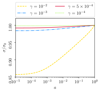
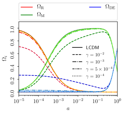
Figure 1: Example of an evolution for $\sigma/\sigma_{0}$ (left panel) and $\Omega_{i}$ (right panel) as function of $a$ for different choices of $\gamma$ for a quartic potential. The value $\sigma_{0}$ of the scalar field at present is fixed consistently with the Cavendish-type measurement of the gravitational constant $G=6.67\times 10^{-8}$ cm³ g^-1 s^-2: $\gamma\sigma_{0}^{2}=\frac{1}{8\pi G}\frac{1+8\gamma}{1+6\gamma}$.

3 The initial conditions

In the following we use the synchronous gauge for metric fluctuations (see Eqs. (1-4) of Ref. [26]) and we denote by $\delta_{i}$ the energy density contrasts, $\theta_{i}=\imath k_{j}v_{i}^{j}$ the velocity potentials and $\sigma_{\nu}$ the neutrino anisotropic pressure. The indices $i=b,\,c,\,\gamma,\,\nu$ denote baryons, CDM, photons, and neutrinos respectively. The scalar field fluctuation is $\delta\sigma$. The perturbed Einstein equations are given by:

$$k^{2}\eta-\frac{1}{2}\mathcal{H}h^{\prime} =-\frac{a^{2}\delta\tilde{\rho}}{2}\,,$$ (3)

$$k^{2}\eta^{\prime} =\frac{a^{2}(\tilde{\rho}+\tilde{P})\tilde{\theta}}{2}\,,$$ (4)

$$h^{\prime\prime}+2\mathcal{H}h^{\prime}-2k^{2}\eta =-3a^{2}\delta\tilde{P}\,,$$ (5)

$$(h^{\prime\prime}+6\eta^{\prime\prime})+2\mathcal{H}(h^{\prime}+6\eta^{\prime})-2k^{2}\eta =-3a^{2}(\tilde{\rho}+\tilde{P})\tilde{\sigma},$$ (6)

where

$$\delta\tilde{\rho}\equiv \frac{\delta\rho_{m}}{\gamma\sigma^{2}}+\frac{h^{\prime}\sigma^{\prime}}{a^{2}\sigma}-\frac{2}{a^{2}}\Biggl{\{}\frac{\delta\sigma^{\prime}}{\sigma}\left(\mathcal{H}-\frac{\sigma^{\prime}}{2\gamma\sigma}\right)+$$

$$+\frac{\delta\sigma}{\sigma}\left[\frac{a^{2}\rho_{m}}{\gamma\sigma^{2}}+\frac{{\sigma^{\prime}}^{2}}{2\gamma\sigma^{2}}+\frac{a^{2}}{\gamma\sigma}\left(\frac{V}{\sigma}-\frac{V,_{\sigma}}{2}\right)-\frac{3\mathcal{H}\sigma^{\prime}}{\sigma}+k^{2}\right]\Biggr{\}},$$

$$(\tilde{\rho}+\tilde{P})\tilde{\theta}\equiv\frac{(\rho_{m}+P_{m})\theta_{m}}{\gamma\sigma^{2}}+\frac{2k^{2}}{a^{2}}\left\{\frac{\delta\sigma}{\sigma}\left[\frac{\sigma^{\prime}}{2\gamma\sigma}(1+2\gamma)-\mathcal{H}\right]+\frac{\delta\sigma^{\prime}}{\sigma}\right\},$$

$$\delta\tilde{P}\equiv \frac{1}{(1+6\gamma)\sigma^{2}}\left(2\delta\rho_{m}+\frac{\delta P_{m}}{\gamma}\right)-\frac{1}{3a^{2}}\Biggl{\{}\frac{3\delta\sigma^{\prime}}{\sigma}\left(2\mathcal{H}-\frac{\sigma^{\prime}}{\gamma\sigma}\right)+$$

$$+\frac{\delta\sigma}{\sigma}\Biggl{[}\frac{6a^{2}P_{m}}{\gamma\sigma^{2}}+\frac{12a^{2}(\rho_{m}-3P_{m})}{(1+6\gamma)\sigma^{2}}+\frac{3\sigma^{\prime}}{\sigma}\left(\frac{\sigma^{\prime}}{\gamma\sigma}-2\mathcal{H}\right)+2k^{2}+$$

$$+\frac{6a^{2}}{(1+6\gamma)}\left(V,_{\sigma\sigma}+\frac{V,_{\sigma}}{2\gamma\sigma}(1-4\gamma)-\frac{V}{\gamma\sigma^{2}}(1-2\gamma)\right)\Biggr{]}+\frac{h^{\prime}\sigma^{\prime}}{\sigma}\Biggr{\}},$$

$$(\tilde{\rho}+\tilde{P})\tilde{\sigma}\equiv\frac{(\rho_{m}+P_{m})\sigma_{m}}{\gamma\sigma^{2}}+\frac{1}{3a^{2}}\left[\frac{4k^{2}\delta\sigma}{\sigma}+2(h^{\prime}+6\eta^{\prime})\frac{\sigma^{\prime}}{\sigma}\right].$$ (7)

Also, the perturbed Klein-Gordon equation is:

$$\delta\sigma^{\prime\prime}=-2\delta\sigma^{\prime}\left(\mathcal{H}+\frac{\sigma^{\prime}}{\sigma}\right)-\delta\sigma\Biggl{[}k^{2}-\frac{{\sigma^{\prime}}^{2}}{\sigma^{2}}+\frac{a^{2}(\rho_{m}-3P_{m})}{(1+6\gamma)\sigma^{2}}+\\ +\frac{a^{2}}{(1+6\gamma)}\left(V,_{\sigma\sigma}+\frac{4V}{\sigma^{2}}-\frac{4V,_{\sigma}}{\sigma}\right)+\frac{a^{2}(\delta\rho_{m}-3\delta P_{m})}{(1+6\gamma)\sigma}-\frac{h^{\prime}\sigma^{\prime}}{2}\Biggr{]}.$$ (8)

The adiabatic plus the new isocurvature solution, in the background considered, is given by:

$$\delta_{\gamma} = \delta_{\nu}=C\left[-\frac{2}{3}k^{2}\tau^{2}+\frac{2\omega}{15}k^{2}\tau^{3}\right]+D\Big{[}-1-\frac{2\omega}{3}\tau+\frac{3(15\gamma+2)\omega^{2}+4k^{2}}{24}\tau^{2}\Big{]}\,,$$

$$\theta_{\gamma} = C\Big{[}-\frac{k^{4}\tau^{3}}{36}+\frac{\omega(5(1+6\gamma){R_{b}}+R_{\gamma})}{240R_{\gamma}}k^{4}\tau^{4}]$$

$$+D\Big{[}-\frac{k^{2}}{4}\tau+\frac{\omega}{48}\left(\frac{9(1+6\gamma)R_{b}}{R_{\gamma}}-4\right)k^{2}\tau^{2}\Big{]}\,,$$

$$\delta_{b} = C\Big{[}-\frac{k^{2}}{2}\tau^{2}+\frac{\omega}{10}k^{2}\tau^{3}\Big{]}+D\Big{[}-\frac{\omega}{2}\tau+\frac{1}{8}\left(\frac{3(15\gamma+2)\omega^{2}}{4k}+k\right)k\tau^{2}\Big{]}\,,$$

$$\delta_{c} = C\Big{[}-\frac{k^{2}}{2}\tau^{2}+\frac{\omega}{10}k^{2}\tau^{3}\Big{]}+D\Big{[}-\frac{1}{2}\omega\tau+\frac{3}{32}(15\gamma+2)\omega^{2}\tau^{2}\Big{]}\,,$$

$$\delta_{\nu} = C\Big{[}-\frac{2}{3}k^{2}\tau^{2}+\frac{2}{15}k^{2}\tau^{3}\omega\Big{]}+D\Big{[}-1-\frac{2\omega}{3}\tau+\frac{3(15\gamma+2)\omega^{2}+4k^{2}}{24}\tau^{2}\Big{]}\,,$$

$$\theta_{\nu} = C\Big{[}-\frac{(4R_{\nu}+23)}{18(4R_{\nu}+15)}k^{4}\tau^{3}+\frac{\omega\left(8R^{2}_{\nu}+60\gamma(5-4R_{\nu})+50{R_{\nu}}+275\right)}{120(2R_{\nu}+15)(4R_{\nu}+15)}k^{4}\tau^{4}\Big{]}$$

$$+D\Big{[}-\frac{1}{4}k^{2}\tau-\frac{1}{12}\omega k^{2}\tau^{2}\Big{]}\,,$$

$$\sigma_{\nu} = C\Big{[}\frac{4k^{2}\tau^{2}}{3(4R_{\nu}+15)}+\frac{(1+6\gamma)(4R_{\nu}-5)\omega k^{2}\tau^{3}}{3(4R_{\nu}+15)(2R_{\nu}+15)}\Big{]}$$

$$+D\Big{[}\frac{k^{2}\tau^{2}}{6(4R_{\nu}+15)}-\frac{2\omega(1+6\gamma)(R_{\nu}+5)k^{2}\tau^{3}}{3(2R_{\nu}+15)(4R_{\nu}+15)}\Big{]}\,,$$

$$h = C\Big{[}k^{2}\tau^{2}-\frac{1}{5}\omega k^{2}\tau^{3}\Big{]}+D\Big{[}\omega\tau-\frac{3}{16}(15\gamma+2)\omega^{2}\tau^{2}\Big{]}\,,$$

$$\eta = C\Big{[}2-\frac{(4R_{\nu}+5)}{6(4{R_{\nu}}+15)}k^{2}\tau^{2}\Big{]}$$

$$+D\Big{[}-\frac{\omega}{6}\tau+\frac{16k^{2}(R_{\nu}+5)+3(15\gamma+2)(4R_{\nu}+15)\omega^{2}}{96(4R_{\nu}+15)}\tau^{2}\Big{]}\,$$

$$\frac{\delta\sigma}{\sigma_{i}} = C\Big{[}-\frac{1}{4}\gamma\omega k^{2}\tau^{3}+\frac{\gamma\omega^{2}}{40}(4+15\gamma)k^{2}\tau^{4}\Big{]}+D\Big{[}-\frac{1}{2}+\frac{3}{4}\gamma\omega\tau\Big{]}\,,$$ (9)

where $\omega\equiv\frac{\rho_{\textup{mat}0}}{\sqrt{3\gamma\rho_{\textup{rad}0}}(1+6\gamma)\sigma_{i}}$ and $\sigma_{i}$ is the value of $\sigma$ deep in the radiation era. In the above equations $C$ ($D$) encodes the primordial power spectrum for curvature (isocurvature) perturbations.

This new mode is present in scalar-tensor theories of gravity and corresponds to a regular growing solution in which the energy densities of the relativistic degrees of freedom and the scalar field compensate at leading order on scales much larger than the Hubble radius, as can be seen by inserting the new solutions for $\delta_{\gamma}\,,\delta_{\nu}$ and $\delta\sigma$ in Eq. (3). This new mode gives a vanishing contribution to the gauge-invariant curvature perturbation in the comoving gauge $\mathcal{R}$ [27] and therefore can be accounted as an isocurvature. To complete the characterization of this new isocurvature mode as done for Einstein gravity [28], we note that the Newtonian potentials, as defined in [26], are given at leading order by $\Psi=-\frac{(R_{\nu}+5)}{(4R_{\nu}+15)}$ and $\Phi=\frac{2(R_{\nu}+5)}{(4R_{\nu}+15)}$.

4 Impact on CMB anisotropies

In order to derive the predictions for the CMB anisotropy angular power spectra we have used an extension to the publicly available Einstein-Boltzmann code CLASS [29, 30], called CLASSig [25]. CLASSig has been developed to derive the predictions for cosmological observables in induced gravity, and more in general scalar-tensor theories, solving for the perturbations but also for the background in order to derive the initial scalar field parameters which provide the cosmology in agreement with the measurements of the gravitational constant in laboratory Cavendish-type experiments. CLASSig has been modified to include the initial conditions for the new isocurvature mode presented. In Fig. 2 we show the comparison of the new mode with the adiabatic and standard isocurvature modes in the $\Lambda$CDM model within Einstein gravity. Fig. 2 also shows the weak dependence of the new isocurvature mode on $\gamma$ at least for the small values consistent with the current cosmological 95%CL upper bound $\gamma\lesssim 0.75\times 10^{-3}$ [21] and for Solar System constraints $\gamma\lesssim 0.6\times 10^{-5}$ [31] .

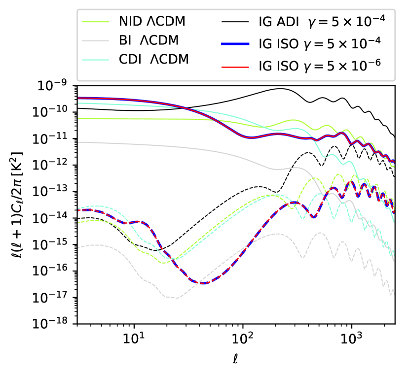
Figure 2: CMB anisotropy angular power spectra in temperature, solid lines, and E-mode polarization, dashed lines. The black curve is the adiabatic case, thin curves represent the three standard $\Lambda$CDM isocurvature modes and the thick curve represent the new isocurvature mode. In order to compare the spectrum shapes we have assumed equal amplitude between isocurvatures and adiabatic mode, i.e. $f_{\mathrm{ISO}}=1$. Note that blue and red lines are superimposed.

The impact of a mixture of curvature and the new isocurvature initial conditions admitting a non-vanishing correlation $\theta$ on CMB anisotropies defined as [32] $C_{\ell}=C_{\ell}^{\mathrm{ADI}}+f_{\mathrm{ISO}}^{2}C_{\ell}^{\mathrm{ISO}}+2f_{\mathrm{ISO}}\cos\theta\,C_{\ell}^{\mathrm{CORR}}$ is displayed in Fig. 3 ($f_{{\mathrm{ISO}}}$ being the relative fraction of isocurvature). Overall, the effect of this new isocurvature mode seems larger and on a wider range of multipoles than the quintessence isocurvature mode in Einstein gravity studied in [9].

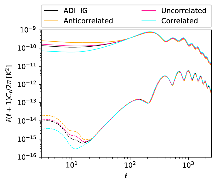
Figure 3: CMB anisotropy angular power spectra in temperature, solid lines, and E-mode polarization, dashed lines, for the three different possibility of correlation between isocurvature and adiabatic modes with $f_{\textup{ISO}}=0.5$ and $n_{\textup{ISO}}=n_{\textup{ADI}}$.

5 Comparison with data

. We now present the constraints on the new isocurvature amplitude with Planck data. Since the effect of isocurvature perturbations on the CMB anisotropy power spectra does not depend significantly on $\gamma$ for $\gamma\lesssim 10^{-3}$ (see Fig. 2), we fix $\gamma=5\times 10^{-4}$ to contain the computational cost of our investigation. Such a value is either compatible with current cosmological observations [25, 21] and conservatively close to the values tested in the comparison of Einstein-Boltzmann codes dedicated to JBD theories reported in [33]. We consider separately the three cases of correlation between adiabatic and isocurvature perturbation $\cos\theta=-1,0,1$ as in [34]. As data we consider Planck 2015 high-$\ell$ temperature likelihood at $\ell\geq 30$ in combination with the joint temperature-polarization likelihood for $2\leq\ell<30$ and the Planck lensing likelihood [35, 36]. To speed up the likelihood evaluation we use the foreground marginalized PlikLite likelihood at high $\ell$ which has been shown in [35] to be in good agreement with minimal extensions of the $\Lambda$CDM model within Einstein gravity. We have also explicitly checked that we can reproduce with PlikLite the constraints obtained with the full Planck high-$\ell$ temperature likelihood in [21].

The modified CLASSig which includes the general initial conditions has been connected to the publicly available code Monte Python [37, 38] to compute the Bayesian probability distribution of cosmological parameters. We vary the baryon density $\omega_{b}=\Omega_{b}h^{2}$, the cold dark matter density $\omega_{c}=\Omega_{c}h^{2}$ (with $h$ being $H_{0}/100{\rm km}\,{\rm s}^{-1}{\rm Mpc}^{-1}$), the reionisation optical depth $\tau_{\mathrm{o}pt}$, the Hubble parameter $H_{0}$ at present time, $\ln(10^{10}A_{S})$, $n_{S}$ and the isocurvature fraction $f_{\mathrm{ISO}}$ with a flat prior [0,0.8]. We sample the posterior using the Metropolis-Hastings algorithm [39] and imposing a Gelman-Rubin convergence criterion [40] of $R-1<0.02$.

We find no evidence at a statistical significant level for this new isocurvature mode. The 95% CL bounds from the MCMC exploration are $f_{\textup{ISO}}<0.07$ for the fully anti-correlated case $\cos\theta=-1$, $f_{\textup{ISO}}<0.12$ for the fully correlated case $\cos\theta=1$ and $f_{\textup{ISO}}<0.31$ for the uncorrelated case $\theta=\pi/2$. These allowed abundances are slightly larger than those of the known isocurvature modes in Einstein gravity , although scale similarly with the degree of correlation [34].

6 Isocurvature perturbations in the effective Newton’s constant from inflation.

We now show that the amplitude of the new isocurvature mode in $\delta\sigma$ compatible with current data could be easily obtained in minimal inflationary models within scalar-tensor gravity. We consider a two-field dynamics in which the scalar field $\sigma\equiv\Phi_{2}$ responsible for the late-time acceleration was present during the inflationary stage driven by the inflaton $\phi\equiv\Phi_{1}$:

$$\!\!\!\!\!\!\!\!\!\!\!\!\!\!S=\int d^{4}x\sqrt{-g}\,\Bigl{[}\frac{\gamma\sigma^{2}R}{2}-\frac{g^{\mu\nu}}{2}\partial_{\mu}\Phi_{i}\partial_{\nu}\Phi_{i}-V(\phi,\sigma)\Bigr{]}\,,$$ (10)

where the indices $i=1,2$ are meant to be summed and $V(\phi,\sigma)=V_{\textup{infl}}(\phi)+V(\sigma)$.

Since $V(\sigma_{0})/(3\gamma\sigma_{0}^{2}H_{0}^{2})\sim 0.7$, $\sigma$ is effectively massless during inflation. We assume that after inflation $\phi$ decays in ordinary matter and dark matter, which are coupled to $\sigma$ only gravitationally through the term $\gamma R\sigma^{2}$. Once the Universe is thermalized, the evolution during the radiation and matter dominated era matches with what previously described for the background and perturbations: indeed, isocurvature perturbations in $\sigma$ are nearly decoupled from curvature perturbations during the radiation dominated period in which $\sigma$ is frozen.

The two field dynamics in Eq. (10) and the corresponding generation of curvature and isocurvature fluctuations have been previously studied [41, 42, 43, 44, 45] either in the original Jordan frame or in the mathematically equivalent Einstein frame. Since in general curvature and isocurvature perturbations are not invariant under conformal transformations [46], we work within the original frame in Eq. (1) consistently with the late time cosmology previously described. Under the assumption that $\sigma$ is subdominant during inflation, we find to lowest order in $\gamma$ and in the slow-roll parameters the isocurvature fraction on scale much larger than the Hubble radius [47]:

$$\frac{\mathcal{P}_{\mathcal{S}}(k_{*})}{\mathcal{P}_{\mathcal{R}}(k_{*})}\simeq\sin^{2}\Delta\,e^{\left(n_{\mathrm{s}}-n_{\mathrm{iso}}\right)(N-N_{*})},$$ (11)

where $n_{\mathrm{s}}$ ($n_{\mathrm{iso}}$) is the tilt of curvature (isocurvature) perturbations, $N_{*}$ is the number of $e$-folds to the end of inflation of the pivot scale $k_{*}$ and $\sin^{2}\Delta$ is the isocurvature relative contribution at Hubble crossing. By considering the scalar tilt consistent with Planck data we use ($n_{S}=0.968\pm 0.06$ at 68% CL [34]) and $[40,\,70]$ as a range for $N_{*}$, we find that the isocurvature fraction at the end of inflation in Eq. (11) can be of the same order of magnitude of the Planck upper bound we obtain.

7 Conclusions

On concluding, we have presented a new growing independent solution in scalar-tensor gravity corresponding to an isocurvature mode between the scalar field which determines the evolution of the effective Newton’s constant and the relativistic degrees of freedom. We have constrained with Planck data this new isocurvature mode when the scalar field is also responsible for the recent acceleration of the Universe and we have shown how this mode can be generated during inflation. It will be interesting to see how the most recent CMB polarization data can further constrain this phenomenological aspect of scalar tensor theories. Work in this direction is in progress.

8 Acknowledgements.

We acknowledge useful discussions with R. Brandenberger, A. Starobinsky and S. Tsujikawa. We acknowledge support by the ”ASI/INAF Agreement 2014-024-R.0 for the Planck LFI Activity of Phase E2”. We also acknowledge financial contribution from the agreement ASI n. I/023/12/0 ”Attivitá relative alla fase B2/C per la missione Euclid”. DP and FF acknowledge financial support by ASI Grant 2016-24-H.0. MB is supported by the South African SKA Project and by the Claude Leon Foundation.

References

- [1] S. Perlmutter et al. [Supernova Cosmology Project Collaboration], Astrophys. J. 517 (1999) 565 doi:10.1086/307221 [astro-ph/9812133].
- [2] A. G. Riess et al. [Supernova Search Team], Astron. J. 116 (1998) 1009 doi:10.1086/300499 [astro-ph/9805201].
- [3] V. Sahni and A. A. Starobinsky, Int. J. Mod. Phys. D 9 (2000) 373 doi:10.1142/S0218271800000542 [astro-ph/9904398].
- [4] P. J. E. Peebles and B. Ratra, Rev. Mod. Phys. 75 (2003) 559 doi:10.1103/RevModPhys.75.559 [astro-ph/0207347].
- [5] T. Clifton, P. G. Ferreira, A. Padilla and C. Skordis, Phys. Rept. 513 (2012) 1 doi:10.1016/j.physrep.2012.01.001 [arXiv:1106.2476 [astro-ph.CO]].
- [6] B. Ratra and P. J. E. Peebles, Phys. Rev. D 37 (1988) 3406. doi:10.1103/PhysRevD.37.3406
- [7] R. R. Caldwell, R. Dave and P. J. Steinhardt, Phys. Rev. Lett. 80 (1998) 1582 doi:10.1103/PhysRevLett.80.1582
- [8] L. R. W. Abramo and F. Finelli, Phys. Rev. D 64 (2001) 083513 doi:10.1103/PhysRevD.64.083513
- [9] T. Moroi and T. Takahashi, Phys. Rev. Lett. 92 (2004) 091301 doi:10.1103/PhysRevLett.92.091301
- [10] C. Gordon and W. Hu, Phys. Rev. D 70 (2004) 083003 doi:10.1103/PhysRevD.70.083003
- [11] F. Perrotta, C. Baccigalupi and S. Matarrese, Phys. Rev. D 61 (1999) 023507.
- [12] T. Chiba, Phys. Rev. D 60 (1999) 083508 doi:10.1103/PhysRevD.60.083508 [gr-qc/9903094].
- [13] J. P. Uzan, Phys. Rev. D 59 (1999) 123510
- [14] N. Bartolo and M. Pietroni, Phys. Rev. D 61 (2000) 023518
- [15] B. Boisseau, G. Esposito-Farese, D. Polarski and A. A. Starobinsky, Phys. Rev. Lett. 85 (2000) 2236.
- [16] C. Baccigalupi, S. Matarrese and F. Perrotta, Phys. Rev. D 62 (2000) 123510 doi:10.1103/PhysRevD.62.123510 [astro-ph/0005543].
- [17] P. Jordan (1955) Schwerkraft und Weltall, Vieweg und Sohn; C. Brans and R. H. Dicke, Phys. Rev. 124 (1961) 925.
- [18] F. Cooper and G. Venturi, Phys. Rev. D 24 (1981) 3338. doi:10.1103/PhysRevD.24.3338
- [19] C. Wetterich, Nucl. Phys. B 302 (1988) 668 doi:10.1016/0550-3213(88)90193-9
- [20] F. Finelli, A. Tronconi and G. Venturi, Phys. Lett. B 659 (2008) 466 doi:10.1016/j.physletb.2007.11.053 [arXiv:0710.2741 [astro-ph]].
- [21] M. Ballardini, F. Finelli, C. Umiltà, and D. Paoletti, JCAP 1605 (2016) no.05, 067 doi:10.1088/1475-7516/2016/05/067 [arXiv:1601.03387 [astro-ph.CO]].
- [22] L. E. Gurevich, A. M. Finkelstein and V. A. Ruban, Astrophys. and Space Sciences 22 (1973) 231
- [23] J. D. Barrow and K. i. Maeda, Nucl. Phys. B 341 (1990) 294. doi:10.1016/0550-3213(90)90272-F
- [24] A. Cerioni, F. Finelli, A. Tronconi and G. Venturi, Phys. Lett. B 681 (2009) 383 doi:10.1016/j.physletb.2009.10.066 [arXiv:0906.1902 [astro-ph.CO]].
- [25] C. Umiltà, M. Ballardini, F. Finelli and D. Paoletti, JCAP 1508 (2015) 017 doi:10.1088/1475-7516/2015/08/017 [arXiv:1507.00718 [astro-ph.CO]].
- [26] C. P. Ma and E. Bertschinger, Astrophys. J. 455 (1995) 7 doi:10.1086/176550 [astro-ph/9506072].
- [27] D. H. Lyth, Phys. Rev. D 31 (1985) 1792. doi:10.1103/PhysRevD.31.1792
- [28] M. Bucher, K. ù and N. Turok, Phys. Rev. D 62 (2000) 083508 doi:10.1103/PhysRevD.62.083508 [astro-ph/9904231].
- [29] J. Lesgourgues, arXiv:1104.2932 [astro-ph.IM].
- [30] D. Blas, J. Lesgourgues and T. Tram, JCAP 1107 (2011) 034.
- [31] B. Bertotti, L. Iess and P. Tortora, Nature 425, 374 (2003). doi:10.1038/nature01997
- [32] L. Amendola, C. Gordon, D. Wands and M. Sasaki, Phys. Rev. Lett. 88 (2002) 211302 doi:10.1103/PhysRevLett.88.211302 [astro-ph/0107089].
- [33] E. Bellini et al., Phys. Rev. D 97 (2018) no.2, 023520 doi:10.1103/PhysRevD.97.023520 [arXiv:1709.09135 [astro-ph.CO]].
- [34] Planck Collaboration, Astron. Astrophys. 594 (2016) A20 doi:10.1051/0004-6361/201525898 [arXiv:1502.02114 [astro-ph.CO]].
- [35] Planck Collaboration, Astron. Astrophys. 594 (2016) A11 doi:10.1051/0004-6361/201526926 [arXiv:1507.02704 [astro-ph.CO]].
- [36] Planck Collaboration, Astron. Astrophys. 594 (2016) A15 doi:10.1051/0004-6361/201525941 [arXiv:1502.01591 [astro-ph.CO]].
- [37] B. Audren, J. Lesgourgues, K. Benabed and S. Prunet, JCAP 1302 (2013) 001.
- [38] T. Brinckmann and J. Lesgourgues, arXiv:1804.07261 [astro-ph.CO].
- [39] W. K. Hastings, Biometrika 57 (1970) 97. doi:10.1093/biomet/57.1.97
- [40] A. Gelman and D. B. Rubin, Statist. Sci. 7 (1992) 457. doi:10.1214/ss/1177011136
- [41] A. A. Starobinsky and J. Yokoyama, Proc. Fourth Workshop on General Relativity and Gravitation eds. K. Nakao et al (Kyoto University, 1995) 381. [gr-qc/9502002].
- [42] J. Garcia-Bellido and D. Wands, Phys. Rev. D 52 (1995) 6739 l doi:10.1103/PhysRevD.52.6739 [gr-qc/9506050].
- [43] A. A. Starobinsky, S. Tsujikawa and J. Yokoyama, Nucl. Phys. B 610 (2001) 383 doi:10.1016/S0550-3213(01)00322-4 [astro-ph/0107555].
- [44] F. Di Marco, F. Finelli and R. Brandenberger, Phys. Rev. D 67 (2003) 063512 doi:10.1103/PhysRevD.67.063512 [astro-ph/0211276].
- [45] F. Di Marco and F. Finelli, Phys. Rev. D 71 (2005) 123502 doi:10.1103/PhysRevD.71.123502 [astro-ph/0505198].
- [46] J. White, M. Minamitsuji and M. Sasaki, JCAP 1207 (2012) 039 doi:10.1088/1475-7516/2012/07/039 [arXiv:1205.0656 [astro-ph.CO]].
- [47] M. Braglia et al., in preparation (2019).