Critically fast pick-and-place with suction cups

Abstract

Fast robotics pick-and-place with suction cups is a crucial component in the current development of automation in logistics (factory lines, e-commerce, etc.). By “critically fast” we mean the fastest possible movement for transporting an object such that it does not slip or fall from the suction cup. The main difficulties are: (i) handling the contact between the suction cup and the object, which fundamentally involves kinodynamic constraints; and (ii) doing so at a low computational cost, typically a few hundreds of milliseconds. To address these difficulties, we propose (a) a model for suction cup contacts, (b) a procedure to identify the contact stability constraint based on that model, and (c) a pipeline to parameterize, in a time-optimal manner, arbitrary geometric paths under the identified contact stability constraint. We experimentally validate the proposed pipeline on a physical robot system: the cycle time for a typical pick-and-place task was less than 5 seconds, planning and execution times included. The full pipeline is released as open-source for the robotics community.

I Introduction

Suction cups have proved to be some of the most robust and versatile devices to grasp a variety of objects, and are therefore used in a large proportion of automation solutions in logistics (factory lines, e-commerce, etc). In addition to robustness and versatility, cycle time is another key driver in the development of automation: how fast automated systems can pick and place objects is a decisive economic question.

In this paper, we are interested in planning and executing critically fast pick-and-place movements with suction cups. By “critically fast” we mean the fastest possible movements for transporting an object such that it does not slip or fall from the suction cup. Another major concern is to also minimize the planning time. Indeed, in a majority of e-commerce scenarios, the robot movements must be computed based on the dynamically perceived positions of the objects to be transported, which implies that both planning and execution times contribute to the total cycle time.

Note that, to focus on the planning and execution aspects, we assume in this paper that the perception problem has been solved upstream: (i) a good model of the environment is available, (ii) the geometries, weight distribution, and initial positions/orientations of the objects are given and accurate.

Essentially, ensuring that the object being transported does not slip or fall amounts to guaranteeing that, at every moment, the net inertial wrench acting on the object can be physically “realized” by its contact with the suction cup (weak contact stability [1, 2]). Since inertial wrenches can be easily computed given a sufficiently accurate model of the object, this task is reduced to identifying the set of wrenches that are physically realizable for the given suction cup contact. A procedure for doing this is among the contributions of this paper. In the following, we will refer to this objective as satisfying the suction cup grasp stability constraint, or simply grasp stability constraint.

In industrial robotic pick-and-place systems, a popular approach to maintaining suction cup grasp stability is to uniformly restrict the robot’s joint velocity and acceleration. The velocity and acceleration limits can be tuned by executing multiple test trajectories, then selecting the set of limits at which there is no failure and the average duration is the shortest. A drawback of this approach is that testing must be done for each object/suction cup combination, and therefore, is tedious and time consuming. Furthermore, it is certain that the resulting movements are not optimal, since the kinematic limits are chosen with respect to all testing trajectories. Also, there is no guarantee that the robot can successfully execute any new, untested trajectory during its actual operation.

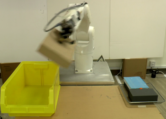
Figure 1: Critically fast pick-and-place of a box with a suction cup. The full video of the experiment is available at https://youtu.be/b9H-zOYWLbY.

An equally important concern is that the computational cost of planning should be small, as otherwise it would undermine the benefit of controlling the robot to move critically fast. For example, suppose one is capable of computing the true time-optimal trajectories, but requires a few seconds per trajectory. In this case, it might be more reasonable to use a sub-optimal approach that has cheaper computational cost, such as limiting the robot’s joint velocity and acceleration. In the same way, the planning procedure needs to be reliable: it has to detect infeasible instances correctly, and is robust against numerical errors.

In this paper, we propose an approach for planning critically fast movements for robotic pick-and-place with suction cups. This approach is computationally efficient and robust, and is verified experimentally to be capable of producing near time-optimal movements. This performance is achieved by means of three main technical contributions:

• A model for suction cup contacts (Section II-C);

• A procedure to compute and approximate the contact stability constraint based on that model (Section II-D);

• A procedure to parameterize, in a time-optimal manner, arbitrary geometric paths under the identified contact stability constraint (Section III).

The full pipeline is available as open-source. Experimental results are reported and discussed in Section IV. A discussion of related works is postponed to Section V.

II Grasp Stability for suction cups

II-A Background 1: Linearized friction cone

In suction cup grasping, frictional forces exist between the suction cup’s pad and the object; these forces are fundamental for maintaining a stable grasp. These frictional forces are modelled using the Colomb friction model. Let $\mathbf{f}=(f_{x},f_{y},f_{z})$ denote a friction force vector, $\mu$ denote the coefficient of friction and let the Z-axis be the normal contact direction, the Colomb friction model states

$$\|(f_{x},f_{y})\|_{2}\leq\mu f_{z}.$$ (1)

The set of feasible friction forces, or equivalently the feasible set of inequality (1), is a Second-Order cone [3] and hence, can be approximated by a polyhedral cone with arbitrary precision [4]. For instance, an approximation with 4 linear inequalities is given as follows:

$$\begin{bmatrix}-1&-1&-\mu\\ -1&1&-\mu\\ 1&1&-\mu\\ 1&-1&-\mu\\ \end{bmatrix}\begin{bmatrix}f_{x}\\ f_{y}\\ f_{z}\end{bmatrix}\leq\mathbf{0}_{4}.$$ (2)

This approximation is known as the linearized friction cone. This is also the approximation we use in this paper.

II-B Background 2: Polyhedral computations

A polytope can be defined as the feasible set of a system of linear equalities and inequalities:

$$\mathbf{A}\mathbf{x}\leq\mathbf{b},\;\mathbf{C}\mathbf{x}=\mathbf{d},$$

where $\mathbf{A},\mathbf{b},\mathbf{C},\mathbf{d}$ are matrices of suitable dimensions. This representation is known as the H-representation, where H stands for halfspace. Alternatively, a polytope can also be defined as the Minkowski sum of the convex hull of a finite number of points and the conic hull of a finite number of rays:

$$\left\{\sum_{i}\theta_{i}\mathbf{u}_{i}\mid\sum_{i}\theta_{i}=1;\forall i,\theta_{i}\geq 0\right\}+\left\{\sum_{i}\theta_{i}\mathbf{v}_{i}\mid\forall i,\theta_{i}\geq 0\right\}.$$

The vertices $\mathbf{u}_{i}$ (resp. rays $\mathbf{v}_{i}$) are referred to as the generating vertices (resp. rays). This representation is known as the V-representation, where V stands for vertex.

A seminal result in the theory of polyhedral computation, discovered by Minkowski and Weyl, is that any polytope has both a H-representation and a V-representation [5]. The problem of computing the V-representation given the H-representation is vertex enumeration; and the dual problem is facet enumeration. Even though both problems are known to be NP-hard, algorithms, such as the Double Description method [5] or the Reversed Search algorithm [6], have been developed to solve them in reasonable times. Both algorithms have publicly available implementations.

II-C Exact suction cup grasp stability constraint

Figure 2: Diagram of a robotic system for pick-and-place. Here $\{O\},\{b\},\{c\}$ denote respectively the global frame, a frame attached to the suction cup and a frame attached to the object. A is a section view shown in Fig. 3.

We model the suction cup-object contact as consisting of multiple point-wise forces: one suction force and $m$ contact point forces  (See Fig. 3). Let $\mathbf{f}^{(0)}$ be the suction force in frame $\{0\}$, which is attached to the centroid of the suction cup, one has:

$$\mathbf{f}^{(0)}_{0}=[0,0,PA]^{\top},$$ (3)

where $P$ is the negative pressure in $\text{\,}\mathrm{P}\mathrm{a}$ and $A$ is the suction area in $\text{\,}\mathrm{m}^{2}$. Let $\mathbf{f}^{(i)}$ denote the $i$-th contact force exerted on the object in the contact local frame. We assume that $\mathbf{f}^{(i)}$ follows the linearized Colomb friction model (2). The suction and contact forces with the corresponding local frames $(\{i\},i=0,\dots,m)$ are depicted in Fig. 3.

Figure 3: Cross-sectional view (cross section A in Fig. 2) of the contact between the cup and the object. The physical contact area is modelled by $m$ point forces following the linearized Colomb friction model and 1 point force capturing the suction force due to negative pressure. A local frame is defined at each point contact.

The net contact wrench exerted on the object by the cup depends linearly on these point forces. Indeed, let $\{c\}$ denote the frame attached rigidly to the suction cup. By transforming all individual forces to frame $\{c\}$ followed by summation, one obtains the net wrench $\mathbf{w}_{c}$:

$$\mathbf{w}_{c}=\sum_{i=0}^{m}\mathbf{G}_{ci}\mathbf{f}_{i}^{(i)},$$ (4)

where the matrix $\mathbf{G}_{ci}$ is a fixed $6\times 3$ matrix that transforms a force in frame $\{i\}$ to a wrench in frame $\{c\}$. We can compute $\mathbf{G}_{ci}$ from the position vector $\mathbf{p}_{ci}$ (position of the origin of frame $\{i\}$ in frame $\{c\}$) and rotational matrix $\mathbf{R}_{ci}$ as below

$$\mathbf{G}_{ci}=\begin{bmatrix}[\mathbf{p}_{ci}\times]\mathbf{R}_{ci}\\ \mathbf{R}_{ci}\end{bmatrix}.$$

We make the following key assumption concerning contact stability for suction cup. This condition is often used in humanoid locomotion [7] and is known as the weak contact stability condition [1].

Assumption 1 (Contact stability).

A contact wrench $\mathbf{w}_{c}$ is physically realizable, and hence allows stable suction-cup object grasp stability, if there exists a set of individual contact forces $\mathbf{f}^{(0)},\dots,\mathbf{f}^{(m)}$ that satisfies Eq. (2) and (3). ∎

An important result that follows from Assump. 1 is that there exists $\mathbf{F}_{c}$ and $\mathbf{g}_{c}$ such that if the contact wrench satisfies

$$\mathbf{F}_{c}\mathbf{w}_{c}\leq\mathbf{g}_{c},$$ (5)

contact stability is achieved. We prove this result by the below constructive procedure, which shows how one can compute $\mathbf{F}_{c}$ and $\mathbf{g}_{c}$ directly:

1. let $\hat{\mathcal{F}}$ be the set of feasible values of $\hat{\mathbf{f}}:=\{\mathbf{f}^{(0)},\dots,\mathbf{f}^{(m)}\}$; form the H-representation of $\hat{\mathcal{F}}$;

2. compute the corresponding V-representation, which is a set of generating vertices $(\hat{\mathbf{f}}_{1},\dots,\hat{\mathbf{f}}_{l})$;

3. use Eq. (4) to transform $(\hat{\mathbf{f}}_{1},\dots,\hat{\mathbf{f}}_{l})$ to $(\hat{\mathbf{w}_{1}},\dots,\hat{\mathbf{w}_{l}})$; $\mathcal{W}_{c}$ is the convex hull of $(\hat{\mathbf{w}_{1}},\dots,\hat{\mathbf{w}_{l}})$;

4. compute the H-representation of $\mathcal{W}_{c}$, which are the coefficient matrices $\mathbf{F}_{c},\mathbf{g}_{c}$ in Eq. (5).

Refer to Section II-B for a discussion on transforming between the two representations (H and V) of a polytope.

II-D Approximate suction cup grasp stability constraint

Figure 4: Application of the procedure proposed (to approximate grasp stability constraint) on a planar data set. Vertices $\hat{\mathbf{w}_{i}}$, guiding samples are shown as gray crosses and red dots respectively. The proposed procedure finds 3 vertices (iter 3) whose convex hull covers the guiding samples completely. The dashed grey polygon, representing the exact constraint, has four times as many edges.

In practice, $\mathbf{F}_{c},\mathbf{g}_{c}$ have many rows, causing computational difficulties. We alleviate this issue by approximating the exact constraint. The key idea is to represent $\mathcal{W}_{c}$ as the convex hull $\mathcal{H}$ of a set of points $\mathcal{Y}$ that (i) belong to $\mathcal{W}_{c}$ and such that (ii) $\mathcal{H}$ contains contact wrenches that are the most likely to be realized during execution. To achieve (ii), we randomly sample guiding samples–contact wrenches that likely occur in execution. This can be done by either sampling real execution data or simulation data.

Concretely, the procedure proceeds as follows:

1. randomly sample $N$ guiding samples; only samples that belongs to $\mathcal{W}_{c}$ are retained;

2. initialize $\mathcal{Y}$ as a simplex with 7 randomly chosen guiding samples as vertices;

3. compute the convex hull $\mathcal{H}$ of $\mathcal{Y}$;

4. choose the face $h^{*}$ of $\mathcal{H}$ that contains the most guiding samples in its infeasible halfspace;

5. add to $\mathcal{Y}$ the vertex in $\mathcal{W}_{c}$ that is in the infeasible halfspace of $h^{*}$ and is furthest away from it;

6. repeat from step 3 until the number of vertices in $\mathcal{Y}$ is greater than a specified value.

Remark that in step 2), since the wrench space is 6 dimensional, a simplex in this space has 7 vertices. After each iteration, a point in $(\hat{\mathbf{w}_{1}},\dots,\hat{\mathbf{w}_{l}})\setminus\mathcal{Y}$ is added to $\mathcal{Y}$. In our experiments, after about 50 iteration, the convex hull $\mathcal{H}$ covers a significant portion of the guiding samples and has approximately $3000$-$4000$ faces. In contrast, $\mathcal{W}_{c}$ can have up to $150000$ faces.

An application of this procedure on a planar data set is demonstrated in Fig. 4. The green triangle, representing the approximate grasp constraint, has only 3 edges but covers all guiding samples.

III Planning critically fast movements

III-A Motion planning pipeline

We propose a motion planning pipeline following the Path-Velocity Decomposition principle [8]:

1. Find a collision-free path using standard geometric planners (e.g. RRT [9]);

2. Time-parameterize the collision-free path to minimize traversal time under kinodynamic constraints: joint velocity bounds, joint acceleration bounds and suction cup constraints.

Although the decoupling approach does not generally produce optimal nor even locally-optimal trajectories, it has the distinctive advantage of being robust and fast. This is due to the highly mature states of collision-free path planning and path time-parameterization techniques [10].

Regarding the latter, the problem of finding the time-optimal time-parameterization of a geometric path subject to kinodynamic constraints is a classical problem in robotics [11]. If the constraints under consideration are of First- or Second-Order (see below and also in [12]), then this problem can be solved extremely efficiently using the recently-developed Time-Optimal Path Parameterization via Reachability Analysis (TOPP-RA) algorithm [12]. Interested readers please refer to the paper [12] or the open-source implementation at https://github.com/hungpham2511/toppra.

In the next section, we show that the grasp stability constraint is a Second-Order constraint.

III-B Grasp stability constraint as Second-Order constraint

A Second-Order constraint has the following form [12]

$$\mathbf{A}(\mathbf{q})\ddot{\mathbf{q}}+\dot{\mathbf{q}}^{\top}\mathbf{B}(\mathbf{q})\dot{\mathbf{q}}+\mathbf{f}(\mathbf{q})\in\mathscr{C}(\mathbf{q}),$$ (6)

• $\mathbf{q}$ is the vector of joint values of the robot;

• $\mathbf{A,B,f}$ are continuous mappings from $\mathbb{R}^{n}$ to $\mathbb{R}^{m\times n},\mathbb{R}^{n\times m\times n}$ and $\mathbb{R}^{m}$ respectively;

• $\mathscr{C}(\bm{\mathrm{q}})$ is a convex polytope in $\mathbb{R}^{m}$.

To establish that any grasp stability constraint can be reformulated as a Second-Order constraint, recall first the following relationships between the robot’s joint position and the object’s motion [13]:

$$\bm{\omega}_{b} =\mathbf{J}_{\rm rot}(\mathbf{q})\dot{\mathbf{q}}, {\bm{\alpha}}_{b} =\mathbf{J}_{\rm rot}(\mathbf{q})\ddot{\mathbf{q}}+\dot{\mathbf{q}}^{\top}\mathbf{H}_{\rm rot}(\mathbf{q})\dot{\mathbf{q}},$$ (7)

$$\mathbf{v}_{b} =\mathbf{J}_{\rm trans}(\mathbf{q})\dot{\mathbf{q}}, \mathbf{a}_{b} =\mathbf{J}_{\rm trans}(\mathbf{q})\ddot{\mathbf{q}}+\dot{\mathbf{q}}^{\top}\mathbf{H}_{\rm trans}(\mathbf{q})\dot{\mathbf{q}},$$ (8)

where $\mathbf{J}_{\Box},\mathbf{H}_{\Box}$ are the translational and rotational Jacobians and Hessians, $\mathbf{v}_{b},\bm{\omega}_{b}$ denote the object’s translational and rotational velocities and $\mathbf{a}_{b},\bm{\alpha}_{b}$ denote the translational and rotational accelerations; all are in the object’s body frame $\{b\}$. Next, combining Eq. (7) and (8) with the Newton and Newton-Euler equations in the body frame, which are

$$\mathbf{w}_{b}+\begin{bmatrix}0_{3}\\ \mathbf{g}_{b}m\end{bmatrix}=\begin{bmatrix}\mathbf{I}_{b}\bm{\alpha}_{b}+\bm{\omega}_{b}\times\mathbf{I}_{b}\bm{\omega}_{b}\\ m\mathbf{a}_{b},\end{bmatrix},$$ (9)

where $m$ is the mass of the object, $\mathbf{w}_{b}$ is the interaction wrench, $\mathbf{g}_{b}$ is gravitational acceleration, $\mathbf{I}_{b}$ is the inertia matrix of the object both in the object’s body frame $\{b\}$. Rearranging the terms of Eq. 9 and substituting in Eq. (7) and (8), one can show that $\mathbf{w}_{b}$ has the form

$$\mathbf{w}_{b}=\Theta_{1}(\mathbf{q})\ddot{\mathbf{q}}+\dot{\mathbf{q}}^{\top}\Theta_{2}(\mathbf{q})\dot{\mathbf{q}}+\Theta_{3}(\mathbf{q}),$$

where $\Theta_{1},\Theta_{2},\Theta_{3}$ are tensors depending on the geometry of the robot and the inertial properties of the object.

Next, let $\mathbf{G}_{cb}$ be the constant matrix that transforms a wrench from the object’s body frame $\{b\}$ to the suction cup’s frame $\{c\}$. Substituting to Eq. (5), grasp stability constraint can then be written as

$$\mathbf{F}_{c}\mathbf{G}_{cb}\left\{\Theta_{1}(\mathbf{q})\ddot{\mathbf{q}}+\dot{\mathbf{q}}^{\top}\Theta_{2}(\mathbf{q})\dot{\mathbf{q}}+\Theta_{3}(\mathbf{q})\right\}\leq\mathbf{g}_{c}.$$ (10)

We can see that Eq. (10) is a Second-Order constraint according to the definition given earlier. Indeed, $\Theta_{1},\Theta_{2},\Theta_{3}$ correspond to matrices $\mathbf{A,B,f}$ respectively and the fixed convex polytope

$$\{\mathbf{w}_{b}\mid\mathbf{F}_{c}\mathbf{G}_{cb}\mathbf{w}_{b}\leq\mathbf{g}_{c}\}.$$

corresponds to $\mathscr{C}(\mathbf{q})$.

IV Experiments

Two aspects of the proposed approach were experimentally investigated. First, we evaluate the quality of the trajectories for transporting object by looking at the rate of successful transport and the trajectories’ durations in 20 randomly generated instances (IV-A). Second, we report the actual computational cost of the proposed pipeline in a realistic pick-and-place scenario (IV-B).

IV-A Experimental setup

The same equipment was employed throughout the experiments. These include a position-controlled industrial robot Denso VS-060, equipped with a suction cup connected to a vacuum pump. The robot is controlled at $125\text{\,}\mathrm{H}\mathrm{z}$. The suction cup has a radius of $12.5\text{\,}\mathrm{m}\mathrm{m}$ and the vacuum pump generates a negative pressure of approximately $30\text{\,}\mathrm{k}\mathrm{P}\mathrm{a}$. Objects considered in the experiments have varying weights ranging from $0.2\text{\,}\mathrm{k}\mathrm{g}$ to $0.6\text{\,}\mathrm{k}\mathrm{g}$; all objects have known weights and moment of inertia. All computations were done on a single core of a laptop running Ubuntu 16.04 at $3.800\text{\,}\mathrm{G}\mathrm{H}\mathrm{z}$.

Collision-free paths between two robot configurations were all computed using OpenRAVE’s implementation [14] of biRRT algorithm [9].

A single Suction Cup stability Constraint (SSC) $\mathbf{F}_{c}\mathbf{w}\leq\mathbf{g}_{c}$ was identified and approximated offline, following the procedure given in Section II. The following parameters were used: $m=6$ points to approximate the suction cup-object contact area; coefficient of friction $\mu=0.3$, identified using a Force-Torque sensor; suction cup radius $12.5\text{\,}\mathrm{m}\mathrm{m}$; maximum $60$ vertices in the V-representation of the constraint (cf. Sec. II-D). The approximated coefficient matrices have $3099$ rows, while the exact coefficient matrices have $130000$ rows. All TOPP instances were discretized with $100$ gridpoints, using the first-order interpolation scheme [12]. The code is written mostly in Python and Cython. TOPP-RA is configured to run a custom LP solver based on Seidel’s algorithm [15].

IV-B Trajectory quality

We first looked at the likelihood of the objects falling, slipping or twisting when executing the trajectories found by our pipeline. As a baseline for comparison, we also considered an alternative strategy, where one computes time-optimal time-parameterizations subject only to the robot’s kinematic constraints, without taking into account the suction cup constraint.

Twenty geometric paths were randomly generated and tested. To mimic actual pick-and-place settings, we adopted the following procedure:

1. sample randomly the object’s starting and goal poses, each in a dedicated region of the workspace;

2. use OpenRAVE’s inverse kinematics to find the corresponding robot’s starting and goal configurations;

3. find a path between the starting and goal configurations using OpenRAVE.

In all trials, a rectangle notebook (See Fig. 5) with weight $0.551\text{\,}\mathrm{k}\mathrm{g}$ and moment of inertia $\mathrm{diag}(9.28,21.10,29.80)\times${10}^{-4}\text{\,}\mathrm{k}\mathrm{g}\mathrm{m}^{2}$$ was transported with the suction cup. The contact point is $12.5\text{\,}\mathrm{m}\mathrm{m}$ above the notebook’s center of mass.

It was found that, by accounting for SCC, the object could be transported without slipping or falling for all 20 paths (Table I). Furthermore, these trajectories were not significantly slower comparing to the robot’s hardware speed limits. On the other hand, only 4 out of 20 trajectories retimed without SSC could be executed successfully. We also observed that 3 in these 4 successful trajectories violate SSC. This could be because the linearized frictional constraint (2) or the approximation procedure in Section II-D are conservative.

Table I: Trajectory duration (in seconds) and success rate of 20 randomly generated trajectories retimed without and with suction cup constraints (SCC).

#	without SCC	with SCC	time ext. (%)
0	0.432 ✗	0.672 ✓	35.71
1	0.568 ✗	0.832 ✓	31.73
2	0.944 ✗	1.008 ✓	6.35
3	0.504 ✗	0.688 ✓	26.74
4	0.728 ✗	0.952 ✓	23.53
5	0.504 ✗	0.672 ✓	25.00
6	1.064 ✓	1.064 ✓	0.00
7	0.520 ✗	0.688 ✓	24.42
8	1.136 ✗	1.344 ✓	15.48
9	0.496 ✗	0.744 ✓	33.33
10	0.632 ✓	0.728 ✓	13.19
11	0.520 ✗	0.648 ✓	19.75
12	0.440 ✗	0.728 ✓	39.56
13	0.824 ✓	0.896 ✓	8.04
14	1.104 ✗	1.392 ✓	20.69
15	0.528 ✗	0.664 ✓	20.48
16	0.520 ✗	0.736 ✓	29.35
17	1.344 ✗	1.848 ✓	27.27
18	0.472 ✗	0.760 ✓	37.89
19	0.512 ✓	0.600 ✓	14.67

A second experiment was performed to examine the degree of sub-optimality. We took paths number 12 and 18, parameterized both subject to grasp stability constraint and executed them at three levels of speed: $100\%,120\%,140\%$. We then inspected the pose of the object relative to the suction cup after each execution. Significant slipping of nearly $1\text{\,}\mathrm{c}\mathrm{m}$ and $10\text{\,}\mathrm{d}\mathrm{e}\mathrm{g}$ were found at the trials executed at $120\%$ and $140\%$ speed, see Fig. 5 and first part of the experimental video https://youtu.be/b9H-zOYWLbY.

Figure 5: Executing a retimed trajectory at $120\%$ and $140\%$ speed led to visible twisting and slipping.

IV-C Computational performance

Table II: Breakdown of task cycle times (in seconds).

	obj 1	obj 2	obj 3	obj 4
APPROACH plan	0.018	0.053	0.016	0.041
REACH plan	0.029	0.034	0.040	0.034
MOVE plan	0.183	0.101	0.147	0.198
MOVE retime	0.111	0.111	0.124	0.137
black!30 Total plan	0.341	0.299	0.327	0.410
black APPROACH exec.	0.438	0.747	0.550	0.531
REACH exec.	0.306	0.368	0.415	0.436
ATTACH delay	1	1	1	1
MOVE exec.	0.841	0.729	1.062	1.371
DETACH delay	1	1	1	1
black!30 Total exec.	3.585	3.844	4.027	4.338
black      Total (plan + exec.)		3.926	4.143	4.354	4.748
black

To investigate the computational cost of the proposed approach, we considered a pick-and-place scenario that involves the robot picking objects using the suction cup from a bin and stacking them at a distant goal position (Fig. 1). The objective is to complete the task as fast as possible, planning and execution time included. The object properties, initial poses and final desired poses were determined prior to the experiment. The objects weighted between $0.204\text{\,}\mathrm{k}\mathrm{g}$ and $0.551\text{\,}\mathrm{k}\mathrm{g}$.

A pick-and-place cycle consisted of several phases. First, the robot approaches a pose that is directly on top of the bin. Then, it reaches for the topmost object, closes the vacuum valve, waits for $1$ second for the object to attach to the suction cup, and finally moves to the given destination. When the robot arrives at the destination, it opens the valve and waits for 1 second for the object to completely detach before starting the next cycle. Note that the waiting times of $1$ second could be reduced.

All collision-free paths were planned online using OpenRAVE. Time-parameterization was also performed online subject to the grasp stability constraint in addition to the robot’s kinematic limits.

The experiment can be visualized in the second part of the experimental video. Table IV-C reports our findings. Pick-and-place cycles were less than $5\text{\,}\mathrm{s}\mathrm{e}\mathrm{c}$ for all objects. On average, the cycle time was $4.29\text{\,}\mathrm{s}\mathrm{e}\mathrm{c}$, of which $0.34\text{\,}\mathrm{s}\mathrm{e}\mathrm{c}$ was for trajectory planning (including path planning and time-parameterization), $1.95\text{\,}\mathrm{s}\mathrm{e}\mathrm{c}$ was for robot motion, and $2\text{\,}\mathrm{s}\mathrm{e}\mathrm{c}$ was for waiting for the pump.

V Related works

In the robotic literature, many researchers have investigated the “waiter problem”: a manipulator, equipped with a flat plate, transports an object that is only placed on the plate. This problem is closely related to the one considered in this paper. A popular approach to achieve grasp stability guarantee, proposed in [16, 17, 18], is to constrain the Zero-tilting Moment Point (ZMP) [19] of the object to its support area on the flat plate. This clearly demonstrates the similarity between object transportation and humanoid locomotion. Similar to the classical ZMP concept for humanoid locomotion, this approach has two limitations: (i) it can only be applied if the object is on a flat surface and (ii) there is no guarantee that the object does not slip or twist [20]. In a more recent work [21], Luo and Hauser proposed to consider the individual contact forces explicitly, eliminating the use of the ZMP and its limitations. However, their formulation resulted in a non-convex non-linear optimization problem that is computationally demanding, taking several seconds to terminate.

In contrast, our proposed approach utilizes polyhedral computational theory [5] to derive grasp stability conditions that can account for general contact configuration (suction cup) and at the same time, allow efficient computations. Our use of polyhedral computational theory is inspired by the development of the Gravito-Inertia Wrench Cone in humanoid locomotion [7].

The motion planning pipeline that we proposed follows the Path-Velocity Decomposition principle [8]. Planning collision-free geometric path, the problem solved in the first stage, is well-understood and can be solved efficiently [22, 23, 24]. Solving Time-Optimal Path Parameterization (TOPP), the problem solved in the second stage, is also a classic problem in robotics [11, 25, 26, 27]. We solve TOPP using TOPP-RA, a recently introduced algorithm that is both highly efficient and robust [12]. Interested readers can refer to [12] for a more comprehensive review of the literature on TOPP.

Lastly, many researchers have presented complete robotic pick-and-place systems [28, 29], offering a broader view of different modules such as motion planning, perception, control and grasping. Regarding motion planning, these reported systems commonly employ reactive strategies that are based on online visual feedback. In contrast, our approach fits entirely in the conventional sense-plan-act strategy. It is clear that with sufficient knowledge of the external environment, our approach can achieve a much higher level of performance; however, it remains to be seen how will it perform in relatively uncertain environments.

VI Conclusion

We have proposed an approach for planning critically fast trajectories for manipulators performing pick-and-place with suction cup. Before execution, we identify the grasp stability constraint, the constraint that the object must not fall from or slip or twist relatively to the suction cup, as a system of linear inequalities. During execution, we plan collision-free geometric paths for transporting objects and retime these paths time-optimally subject to the identified grasp stability constraint using the TOPP-RA algorithm.

Experiments were conducted to assess the performance of the proposed approach. The results suggest that the approach is capable of producing high-quality trajectories: these trajectories can be executed successfully without causing the object to fall or slip and have duration that were close to the true time-optimal values. Further, the proposed approach has a low computational cost, making it suitable for online motion planning for industrial applications.

There are two limitations that we are actively investigating:

• Our approach requires exact knowledge of the object’s inertial properties: center-of-mass position, mass and moment of inertia and the robot’s geometry. Yet, in practice, identification and modelling errors always exist; only approximations of objects’ properties are available. This observation leads to two questions: 1) what are the effects of identification errors on motion quality and 2) how to handle these errors;

• The approximation step presented in Section II-D reduces computational time significantly as the size of the grasp stability constraint is much smaller. However, its effects on motion quality is, in general, not completely understood.

Acknowledgment

This work was partially supported by the Medium-Sized Centre funding scheme (awarded by the National Research Foundation, Prime Minister’s Office, Singapore).

References

- [1] J.-S. Pang and J. Trinkle, “Stability characterizations of rigid body contact problems with coulomb friction,” ZAMM-Journal of Applied Mathematics and Mechanics/Zeitschrift für Angewandte Mathematik und Mechanik, vol. 80, no. 10, pp. 643–663, 2000.
- [2] S. Caron, Q.-C. Pham, and Y. Nakamura, “Stability of surface contacts for humanoid robots: Closed-form formulae of the contact wrench cone for rectangular support areas,” in 2015 IEEE International Conference on Robotics and Automation (ICRA). IEEE, 2015, pp. 5107–5112.
- [3] S. Boyd and L. Vandenberghe, Convex Optimization. New York, NY, USA: Cambridge University Press, 2004.
- [4] a. Ben-Tal and a. Nemirovski, “On Polyhedral Approximations of the Second-Order Cone,” Mathematics of Operations Research, 2001.
- [5] K. Fukuda and A. Prodon, “Double description method revisited,” in Combinatorics and computer science. Springer, 1996, pp. 91–111.
- [6] D. Avis and K. Fukuda, “Reverse search for enumeration,” Discrete Applied Mathematics, 1996.
- [7] S. Caron, Q.-C. Pham, and Y. Nakamura, “ZMP Support Areas for Multicontact Mobility Under Frictional Constraints,” IEEE Transactions on Robotics, vol. 33, no. 1, pp. 67–80, feb 2017.
- [8] K. Kant and S. W. Zucker, “Toward efficient trajectory planning: The path-velocity decomposition,” The international journal of robotics research, vol. 5, no. 3, pp. 72–89, 1986.
- [9] J. J. Kuffner and S. M. LaValle, “RRT-connect: An efficient approach to single-query path planning,” in Robotics and Automation, 2000. Proceedings. ICRA’00. IEEE International Conference on, vol. 2. IEEE, 2000, pp. 995–1001.
- [10] Q.-C. Pham, S. Caron, P. Lertkultanon, and Y. Nakamura, “Admissible velocity propagation: Beyond quasi-static path planning for high-dimensional robots,” The International Journal of Robotics Research, vol. 36, no. 1, pp. 44–67, 2017.
- [11] J. E. Bobrow, S. Dubowsky, and J. S. Gibson, “Time-optimal control of robotic manipulators along specified paths,” The international journal of robotics research, vol. 4, no. 3, pp. 3–17, 1985.
- [12] H. Pham and Q. C. Pham, “A New Approach to Time-Optimal Path Parameterization Based on Reachability Analysis,” IEEE Transactions on Robotics, vol. 34, no. 3, pp. 645–659, 2018. [Online]. Available: https://arxiv.org/abs/1707.07239
- [13] a. Hourtash, “The Kinematic Hessian and Higher Derivatives,” 2005 International Symposium on Computational Intelligence in Robotics and Automation, 2005.
- [14] R. Diankov and J. Kuffner, “OpenRAVE : A Planning Architecture for Autonomous Robotics,” Robotics, no. July, pp. –34, 2008. [Online]. Available: http://www.ri.cmu.edu/pub_files/pub4/diankov_rosen_2008_2/diankov_rosen_2008_2.pdf
-
[15]
R. Seidel, “Small-dimensional linear programming and convex hulls made
easy,” Discrete & Computational Geometry, vol. 6, no. 3, pp.
423–434, 1991.
- [16] P. Lertkultanon and Q. C. Pham, “Dynamic non-prehensile object transportation,” in 2014 13th International Conference on Control Automation Robotics and Vision, ICARCV 2014. IEEE, 2014, pp. 1392–1397.
- [17] F. G. Flores and A. Kecskeméthy, “Time-optimal path planning for the general waiter motion problem,” in Mechanisms and Machine Science, V. Kumar, J. Schmiedeler, S. V. Sreenivasan, and H.-J. Su, Eds. Heidelberg: Springer International Publishing, 2013, vol. 14, pp. 189–203. [Online]. Available: https://doi.org/10.1007/978-3-319-00398-6_14
- [18] G. Csorvási, Á. Nagy, and I. Vajk, “Near Time-Optimal Path Tracking Method for Waiter Motion Problem,” IFAC-PapersOnLine, vol. 50, no. 1, pp. 4929–4934, 2017.
- [19] M. Vukobratović and B. Borovac, “Zero-Moment Point — Thirty Five Years of Its Life,” International Journal of Humanoid Robotics, vol. 01, no. 01, pp. 157–173, 2004.
- [20] P. Sardain and G. Bessonnet, “Forces acting on a biped robot. Center of pressure-zero moment point,” IEEE Transactions on Systems, Man, and Cybernetics-Part A: Systems and Humans, vol. 34, no. 5, pp. 630–637, 2004.
- [21] J. Luo and K. Hauser, “Robust trajectory optimization under frictional contact with iterative learning,” Autonomous Robots, vol. 41, no. 6, pp. 1447–1461, 2017.
- [22] S. M. LaValle, “Randomized Kinodynamic Planning,” The International Journal of Robotics Research, no. September, 2001.
- [23] R. Bordalba, L. Ros, and J. M. Porta, “Randomized kinodynamic planning for constrained systems,” in 2018 IEEE International Conference on Robotics and Automation (ICRA). IEEE, 2018, pp. 7079–7086.
- [24] M. Zucker, N. Ratliff, A. D. Dragan, M. Pivtoraiko, M. Klingensmith, C. M. Dellin, J. A. Bagnell, and S. S. Srinivasa, “CHOMP: Covariant Hamiltonian optimization for motion planning,” The International Journal of Robotics Research, vol. 32, no. 9-10, pp. 1164–1193, 2013.
- [25] D. Verscheure, B. Demeulenaere, J. Swevers, J. De Schutter, and M. Diehl, “Practical time-optimal trajectory planning for robots: a convex optimization approach,” IEEE Transactions on Automatic Control, 2008.
- [26] K. Hauser, “Fast interpolation and time-optimization with contact,” The International Journal of Robotics Research, vol. 33, no. 9, pp. 1231–1250, aug 2014.
- [27] Q.-C. Pham, “A General, Fast, and Robust Implementation of the Time-Optimal Path Parameterization Algorithm,” IEEE Transactions on Robotics, vol. 30, no. 6, pp. 1533–1540, dec 2014.
- [28] N. Correll, K. E. Bekris, D. Berenson, O. Brock, A. Causo, K. Hauser, K. Okada, A. Rodriguez, J. M. Romano, and P. R. Wurman, “Analysis and Observations from the First Amazon Picking Challenge,” IEEE Transactions on Automation Science and Engineering, 2016. [Online]. Available: http://arxiv.org/abs/1601.05484
- [29] D. Morrison, A. W. Tow, M. McTaggart, R. Smith, N. Kelly-Boxall, S. Wade-McCue, J. Erskine, R. Grinover, A. Gurman, and T. Hunn, “Cartman: The low-cost cartesian manipulator that won the amazon robotics challenge,” arXiv preprint arXiv:1709.06283, 2017.