Maximum Pairwise Bayes Factors for Covariance Structure Testing

Abstract

Hypothesis testing of structure in covariance matrices is of significant importance, but faces great challenges in high-dimensional settings. Although consistent frequentist one-sample covariance tests have been proposed, there is a lack of simple, computationally scalable, and theoretically sound Bayesian testing methods for large covariance matrices. Motivated by this gap and by the need for tests that are powerful against sparse alternatives, we propose a novel testing framework based on the maximum pairwise Bayes factor. Our initial focus is on one-sample covariance testing; the proposed test can optimally distinguish null and alternative hypotheses in a frequentist asymptotic sense. We then propose diagonal tests and a scalable covariance graph selection procedure that are shown to be consistent. A simulation study evaluates the proposed approach relative to competitors. We illustrate advantages of our graph selection method on a gene expression data set.

Key words: Bayesian hypothesis test, covariance matrix, modularization

1 Introduction

Consider a sample of observations from a high-dimensional normal model

$$X_{1},\ldots,X_{n}\mid\Sigma_{n} \overset{i.i.d.}{\sim} N_{p}(0,\Sigma_{n}),$$ (1)

where $\Sigma_{n}\in\mathbb{R}^{p\times p}$ is a covariance matrix. There is often interest in inferring the structure in $\Sigma_{n}$ and in comparing different alternative covariance structures. This article focuses on this problem from a hypothesis testing perspective. Let $X=(X_{1},\ldots,X_{n})^{T}\in\mathbb{R}^{n\times p}$ be the data matrix. A one-sample covariance test can be reduced to the following simple form:

$$H_{0}:\Sigma_{n}=I_{p}\quad\text{versus}\quad H_{1}:\Sigma_{n}\neq I_{p},$$ (2)

by noting that $H_{0}:\Sigma_{n}=I_{p}$ is equivalent to a null hypothesis $H_{0}:\Sigma_{n}=\Sigma_{0}$ for any given positive definite matrix $\Sigma_{0}$ by applying the linear transformation $X_{i}\mapsto\Sigma_{0}^{-1/2}X_{i}$.

Another important problem is testing diagonality

$$H_{0}:\sigma_{ij}=0\text{ for any }i\neq j\quad\text{ versus }\quad H_{1}:\text{ not }H_{0},$$

where $\Sigma_{n}=(\sigma_{ij})$. Finally, we consider the problem of support recovery, corresponding to estimating the nonzero elements of covariance matrices.

We are interested in constructing novel Bayesian procedures that are practically applicable with theoretical guarantees for the (i) one-sample covariance test, (ii) diagonality test, and (iii) support recovery of the covariance matrix. We consider the high-dimensional setting in which the number of variables $p$ can grow to infinity as the sample size $n$ gets larger and possibly be much larger than $n$. Although it is well known that assuming a restricted covariance class is necessary for consistent estimation of large covariance matrices (Johnstone and Lu, 2009; Lee and Lee, 2018), in a testing context we focus on alternative hypotheses $H_{1}$ that are unconstrained. One natural possibility is to assume a conjugate inverse-Wishart prior $IW_{p}(\nu_{n},A_{n})$ for $\Sigma_{n}$ under $H_{1}$. However, in order for the resulting posterior to be proper, it is necessary to choose the degrees of freedom $\nu_{n}>p-1$, suggesting an extremely informative prior in high-dimensional settings. The resulting test will certainly be highly sensitive to the choice of $A_{n}$, and hence is not very useful outside of narrow applications having substantial prior information. One could instead choose a non-conjugate prior for $\Sigma_{n}$ under $H_{1}$, but then substantial computational issues arise in attempting to estimate the Bayes factor.

From a frequentist perspective, Chen et al. (2010) and Cai and Ma (2013) suggested consistent one-sample covariance tests based on unbiased estimators of $\|\Sigma_{n}-I_{p}\|_{F}^{2}$, where $\|A\|_{F}=\big{(}\sum_{ij}a_{ij}^{2}\big{)}^{1/2}$ is the Frobenius norm of a matrix $A=(a_{ij})$. Under the null hypothesis, they showed that their test statistic is asymptotically normal. The test also has power tending to one as $n$ goes to infinity, but it requires the condition, $\|\Sigma_{n}-I_{p}\|_{F}^{2}\,n/p\to\infty$ as $n\to\infty$. This condition implies that they essentially adopted $H_{1}=\{\Sigma_{n}:\|\Sigma_{n}-I_{p}\|_{F}^{2}\geq b_{n}p/n\}$ for some $b_{n}\to\infty$ as $n\to\infty$ as the alternative class. Cai and Ma (2013) proved that if we consider an alternative class $H_{1}=\{\Sigma_{n}:\|\Sigma_{n}-I_{p}\|_{F}^{2}\geq\epsilon_{n}\}$, say a dense alternative, the condition $\epsilon_{n}\geq b_{n}p/n$ is inevitable for any level $\alpha$ test to have power tending to one. This excludes cases in which a finite number of the components of $\Sigma_{n}-I_{p}$ have a magnitude $(p/n)^{1/2}$, although $(p/n)^{1/2}$ can be a significant signal when $p\geq n$.

The above discussion motivates us to develop hypothesis tests that are easy to implement in practice while possessing theory guarantees. In particular, we wish to construct tests that can perform well even when the condition $\|\Sigma_{n}-I_{p}\|_{F}^{2}\,n/p\to\infty$ fails to hold. We achieve this by proposing a novel Bayesian testing framework based on the maximum pairwise Bayes factor which will be introduced in Section 2.2. The basic strategy is to focus on the pairwise difference between $\Sigma_{n}$ and $I_{p}$ rather than the Frobenius norm or other matrix norms. More precisely, instead of considering a usual Bayes factor based on a prior on the whole covariance matrix, we first consider the pairwise Bayes factors for each element of the matrix and combine them by taking a maximum over all possible pairs. This approach is analagous to frequentist tests based on maximum-type statistics (Jeng et al., 2013; Enikeeva and Harchaoui, 2019). Our construction enables us to consider a different alternative class, $H_{1}=\{\Sigma_{n}:\|\Sigma_{n}-I_{p}\|_{\max}^{2}\geq C\log p/n\}$ for some constant $C>0$, say a sparse alternative, where $\|A\|_{\max}=\max_{i,j}|a_{ij}|$ for a matrix $A=(a_{ij})$. When the primary interest is not on a collection of very weak signals, but on detecting at least one meaningful signal, our test is much more effective than the frequentist methods mentioned above.

The proposed testing method is general, easily implementable and theoretically supported, being the first Bayesian test shown to be consistent in the high-dimensional setting for the one-sample or diagonal covariance testing problems. Our procedure yields proven false discovery rate control and power improvement compared to existing methods. The proposed one-sample test is rate-optimal in the sense that it can distinguish the sparse alternative class $H_{1}=\{\Sigma_{n}:\|\Sigma_{n}-I_{p}\|_{\max}^{2}\geq\epsilon_{n}\}$ from the null with the fastest rate of $\epsilon_{n}$, while guaranteeing consistency under the null. We also propose a scalable graph selection method for high-dimensional covariance graph models using pairwise Bayes factors. The proposed method consistently recovers the true covariance graph structure under a weaker or comparable condition to those in the existing frequentist literature.

Recently, Leday and Richardson (2018) suggested a fundamentally different pairwise approach to test marginal or conditional independence between two variables. Their focus is on the joint distribution of the $i$th and $j$th variables and an inverse-Wishart prior for $\Sigma_{n}$ was imposed. For each $i\neq j$, the hypothesis testing problem $H_{0,ij}^{M}:\sigma_{ij}=0$ versus $H_{1,ij}^{M}:\sigma_{ij}\neq 0$ was considered. Since the resulting Bayes factors for the pairwise tests are not scale-invariant, they proposed scaled versions. P-values under the conditional null distribution were obtained by shuffling or permuting labels of observations (Jiang et al., 2017). For support recovery, they suggest using standard multiplicity correction procedures to control the false discovery rate, obtaining a frequentist procedure. Selection consistency results were not provided.

R code for implementation of our empirical results are available at https://github.com/leekjstat/mxPBF. Proofs of our main results are included in Supplementary Material.

2 Preliminaries

2.1 Notations

For any real values $a$ and $b$, we denote $a\vee b$ as the maximum between $a$ and $b$. For any positive sequences $a_{n}$ and $b_{n}$, we denote $a_{n}\ll b_{n}$ or $a_{n}=o(b_{n})$ if $a_{n}/b_{n}\to 0$ as $n\to\infty$. For any vector $x=(x_{1},\ldots,x_{p})^{T}\in\mathbb{R}^{p}$, we define the vector $\ell_{1}$- and $\ell_{2}$-norm as $\|x\|_{1}=\sum_{j=1}^{p}|x_{i}|$ and $\|x\|_{2}=(\sum_{j=1}^{p}x_{j}^{2})^{1/2}$, respectively. Let $\mathcal{C}_{p}$ be the set of all $p\times p$ positive definite matrices. We denote $\chi_{k}^{2}(\lambda)$ as the non-central chi-square distribution with degrees of freedom $k$ and non-centrality $\lambda\geq 0$, and let $\chi_{k}^{2}=\chi_{k}^{2}(\lambda=0)$. For positive real values $a$ and $b$, $IG(a,b)$ denotes the inverse gamma distribution with shape $a$ and scale $b$.

2.2 Maximum Pairwise Bayes Factor

In this subsection, we introduce our approach focusing on the one-sample covariance test. As described before, the basic strategy is to concentrate on the pairwise difference between $\Sigma_{n}$ and $I_{p}$. Let $\tilde{X}_{j}\in\mathbb{R}^{n}$ be the $j$th column vector of $X$. For any indices $i$ and $j$, based on the joint distribution (1), the conditional distribution of $\tilde{X}_{i}$ given $\tilde{X}_{j}$ is

$$\tilde{X}_{i}\mid\tilde{X}_{j} \sim N_{n}\Big{(}a_{ij}\tilde{X}_{j},\,\tau_{ij}^{2}I_{n}\Big{)},$$ (3)

where $a_{ij}\in\mathbb{R}$ and $\tau_{ij}>0$. We can view (3) as a linear regression model given a design matrix $\tilde{X}_{j}$. For each paired conditional model (3), we consider a testing problem

$$H_{0,ij}:a_{ij}=0,\,\tau_{ij}^{2}=1\quad\text{versus}\quad H_{1,ij}:\text{ not }H_{0,ij}.$$ (4)

If $H_{0,ij}$ is true, $\sigma_{ij}=0$ and $\sigma_{ii}=1$ because $a_{ij}=\sigma_{ij}/\sigma_{jj}$ and $\tau_{ij}^{2}=\sigma_{ii}(1-\rho_{ij}^{2})$, where $\Sigma_{n}=(\sigma_{ij})$ and $R_{n}=(\rho_{ij})$ are covariance and correlation matrices, respectively. We suggest the following prior distribution under the alternative hypothesis $H_{1,ij}$ in (4),

$$\begin{split}a_{ij}\mid\tau_{ij}^{2}\,\,\sim\,\,N\Big{(}0,\,\frac{\tau_{ij}^{2}}{\gamma}\|\tilde{X}_{j}\|_{2}^{-1}\Big{)},&\quad\,\tau_{ij}^{2}\,\,\sim\,\,IG\big{(}a_{0},\,b_{0,ij}\big{)},\end{split}$$ (5)

where $\gamma=(n\vee p)^{-\alpha}$ and $a_{0},b_{0,ij}$ and $\alpha$ are positive constants. The induced Bayes factor is

$$B_{10}(\tilde{X}_{i},\tilde{X}_{j}) = \frac{p(\tilde{X}_{i}\mid\tilde{X}_{j},H_{1,ij})}{p(\tilde{X}_{i}\mid\tilde{X}_{j},H_{0,ij})}$$

$$= \frac{b_{0,ij}^{a_{0}}}{\Gamma(a_{0})}\Big{(}\frac{\gamma}{1+\gamma}\Big{)}^{1/2}\Gamma\Big{(}\frac{n}{2}+a_{0}\Big{)}\,e^{n\widehat{\tau}_{i}^{2}/2}\,\Big{(}\frac{n}{2}\widehat{\tau}_{ij,\gamma}^{2}+b_{0,ij}\Big{)}^{-n/2-a_{0}},$$

where $n\widehat{\tau}_{i}^{2}=\|\tilde{X}_{i}\|_{2}^{2}$, $n\widehat{\tau}_{ij,\gamma}^{2}=\tilde{X}_{i}^{T}\{I_{n}-(1+\gamma)^{-1}H_{j}\}\tilde{X}_{i}$ and $H_{j}=\tilde{X}_{j}(\tilde{X}_{j}^{T}\tilde{X}_{j})^{-1}\tilde{X}_{j}^{T}$. The choice of hyperparameters $a_{0}$ and $b_{0,ij}$ is discussed in Section 4.1.

The null hypothesis in the one-sample covariance test, $H_{0}:\Sigma_{n}=I_{p}$, is true if $H_{0,ij}$ is true for all pairs $(i,j)$ such that $i\neq j$. We aggregate the information from each pairwise Bayes factor $B_{10}(\tilde{X}_{i},\tilde{X}_{j})$ via the maximum pairwise Bayes factor,

$$B_{\max,10}(X) = \max_{i\neq j}B_{10}(\tilde{X}_{i},\tilde{X}_{j}).$$ (6)

A large value for $B_{\max,10}(X)$ provides evidence supporting the alternative hypothesis. By taking a maximum, $B_{\max,10}(X)$ supports the alternative hypothesis if at least one of the pairwise Bayes factors supports the alternative. A natural question is whether false positives increase as we take a maximum over more and more pairs. Indeed, we find that this is not the case, either asymptotically based on our consistency results (Theorems 1 and 3) or in finite samples based on simulations.

3 Main Results

3.1 One-sample Covariance Test

In this subsection, we show consistency of $B_{\max,10}(X)$ defined in (6) for the one-sample covariance test (2). We first introduce assumptions for consistency under $H_{1}:\Sigma_{n}\neq I_{p}$. Let $\Sigma_{0}=(\sigma_{0,ij})\in\mathcal{C}_{p}$ be the true covariance matrix, implying the conditional distribution of $\tilde{X}_{i}$ given $\tilde{X}_{j}$ is

$$\tilde{X}_{i}\mid\tilde{X}_{j} \sim N_{n}\big{(}a_{0,ij}\tilde{X}_{j},\tau_{0,ij}^{2}I_{n}\big{)}$$ (7)

under $\mathbb{P}_{0}$, where $a_{0,ij}=\sigma_{0,ij}/\sigma_{0,jj}$, $\tau_{0,ij}^{2}=\sigma_{0,ii}\{1-\sigma_{0,ij}^{2}/(\sigma_{0,ii}\sigma_{0,jj})\}$, $\mathbb{P}_{0}$ is the probability measure corresponding to model (1) with $\Sigma_{n}=\Sigma_{0}$, and $\tau_{0,ij}^{2}=\sigma_{0,ii}$ if and only if $a_{0,ij}=0$. Under the alternative $H_{1}:\Sigma_{n}\neq I_{p}$, we assume that $\Sigma_{0}$ satisfies at least one of the following conditions:

• There exists a pair $(i,j)$ satisfying

  $$\big{|}\sigma_{0,ii}-1\big{|} \geq \Big{[}4\sigma_{0,ii}{C_{1}}^{1/2}+C_{2}+\frac{2b_{0,ij}}{\{n\log(n\vee p)\}^{1/2}}\Big{]}\left\{\frac{\log(n\vee p)}{n}\right\}^{1/2}$$ (8)

  for some constants $C_{1}>0$ and $C_{2}>2(\alpha+2)^{1/2}$.

• There exists a pair $(i,j)$ satisfying

  $$\big{|}\tau_{0,ij}^{2}-1\big{|} \geq \Big{[}4\tau_{0,ij}^{2}{C_{1}}^{1/2}+C_{2}+\frac{2b_{0,ij}+\tau_{0,ij}^{2}}{\{n\log(n\vee p)\}^{1/2}}\Big{]}\left\{\frac{\log(n\vee p)}{n}\right\}^{1/2}$$ (9)

• There exists a pair $(i,j)$ satisfying

  $$\sigma_{0,ij}^{2} \geq \frac{\sigma_{0,jj}}{1-2{C_{1}}^{1/2}\epsilon_{0}}\left\{\frac{9C_{1}\tau_{0,ij}^{2}}{(1-C_{3})^{2}}\vee\frac{C_{4}(\alpha+2)}{C_{3}}\right\}\frac{\log(n\vee p)}{n}\quad\quad$$ (10)

  for some constants $0<C_{3}<1$ and $C_{4}>1$.

Throughout the paper, $C_{1},C_{2},C_{3}$ and $C_{4}$ are fixed global constants. For a given small constant $\epsilon>0$, they can be considered as $C_{1}=\epsilon,C_{2}=2(\alpha+2)^{1/2}+\epsilon,C_{3}=1-\epsilon^{1/4}$ and $C_{4}=1+\epsilon$.

Condition (A1) is required to detect a non-unit variance $\sigma_{0,ii}$, and can be interpreted as a beta-min condition for $|\sigma_{0,ii}-1|$. The beta-min condition gives a lower bound for nonzero parameters and is essential for model selection consistency (Castillo et al., 2015; Martin et al., 2017). Interestingly, the rate of lower bound in (A1) is given by $\{\log(n\vee p)/n\}^{1/2}$, which has been commonly used in the variable selection literature. Condition (A2) is similar to condition (A1), which can be interpreted as a beta-min condition for $|\tau_{0,ij}^{2}-1|$. Condition (A3) is a beta-min condition for off-diagonal elements of the covariance matrix. In summary, conditions (A1)–(A3) imply the sparse alternative

$$\Sigma_{0} \in H_{1}\,=\,\Big{\{}\,\Sigma_{n}:\|\Sigma_{n}-I_{p}\|_{\max}^{2}\geq C\,\frac{\log p}{n}\,\Big{\}}$$

for some constant $C>0$, which corresponds to the meaningful difference we mentioned earlier. In fact, the rate $\log p/n$ is optimal for guaranteeing the consistency under both hypotheses (Theorem 2). Our method is not designed to detect dense alternatives in which all differences are very small, but requires at least one difference to be sufficiently large.

Theorem 1 shows consistency for the one-sample covariance test even in the high-dimensional setting as long as $\log p\leq\epsilon_{0}^{2}n$ for some small constant $\epsilon_{0}>0$.

Theorem 1

Consider model (1) and the one-sample covariance testing problem (2). Consider prior (5) under $H_{1,ij}$ in (4) with $\alpha>8(1+{2}^{1/2}\epsilon_{0})^{2}/\{1-{2}^{3/2}\epsilon_{0}(1+{2}^{1/2}\epsilon_{0})\}$ for some small constant $0<\epsilon_{0}<3\,(4C_{2})^{-1}$. Assume that $\log p\leq\epsilon_{0}^{2}\,n$ for all large $n$. Then under $H_{0}:\Sigma_{n}=I_{p}$, for some constant $c>0$,

$$B_{\max,10}(X) = O_{p}\big{\{}(n\vee p)^{-c}\big{\}}.$$

If, under $H_{1}:\Sigma_{n}\neq I_{p}$, $\Sigma_{0}$ satisfies at least one of conditions (A1)–(A3), for some constant $c^{\prime}>0$,

$$B_{\max,10}(X)^{-1} = O_{p}\big{\{}(n\vee p)^{-c^{\prime}}\big{\}}.$$

We first prove that the pairwise Bayes factor $B_{10}(\tilde{X}_{i},\tilde{X}_{j})$ is consistent on a large event $E_{ij}$ such that $\mathbb{P}_{0}(E_{ij}^{c})\to 0$ as $n\to\infty$. To show consistency under $H_{0}$, it suffices to prove that $\sum_{i\neq j}\mathbb{P}_{0}(E_{ij}^{c})\to 0$ as $n\to\infty$, which means that the false discovery rate converges to zero. The condition for $\alpha$ in Theorem 1 is closely related to this requirement. It also has connections with the variable selection literature in regression (Fernandez et al., 2001; Narisetty and He, 2014; Yang et al., 2016) where the prior dispersion needs to depend on $(n\vee p^{2})$ or $p$ for consistency. Our theory requires a larger dispersion of order roughly $(n\vee p)^{8}$ mainly due to the larger number of parameters compared to the regression setting.

To show consistency under $H_{1}$, it suffices to show $\mathbb{P}_{0}(E_{ij}^{c})\to 0$ as $n\to\infty$ for some index $(i,j)$ satisfying at least one of conditions (A1)–(A3). Interestingly, the rate of convergence is similar under both hypotheses, unlike most Bayesian testing procedures with the notable exception of non-local prior based methods (Johnson and Rossell, 2010, 2012).

The next theorem shows the optimality of the alternative class which is considered in Theorem 1 (Conditions (A1)–(A3)). It says, when the alternative class is defined based on the element-wise maximum norm, the condition $\|\Sigma_{0}-I_{p}\|_{\max}^{2}\geq C\log p/n$ for some constant $C>0$ is necessary for any consistent test to have power tending to one. Thus, conditions (A1)–(A3) are rate-optimal to guarantee the consistency under $H_{0}$ as well as $H_{1}$.

Theorem 2

Let $E_{\Sigma}$ be the expectation corresponding to model (1). For a given constant $C_{\star}>0$, define $H_{1}(C_{\star})=\Big{\{}\Sigma\in\mathcal{C}_{p}:\|\Sigma-I_{p}\|_{\max}^{2}\geq C_{\star}^{2}\log p/n\Big{\}}.$ If $C_{\star}^{2}\leq 2$, then for any consistent test $\phi$ such that $E_{I_{p}}\phi\longrightarrow 0$ as $n\to\infty$,

$$\limsup_{n\to\infty}\inf_{\Sigma\in H_{1}(C_{\star})}E_{\Sigma}(\phi)\leq\frac{1}{2}.$$

3.2 Testing Diagonality

We now consider testing of diagonality of the covariance matrix:

$$H_{0}:\sigma_{ij}=0\text{ for any }i\neq j\quad\text{ versus }\quad H_{1}:\text{ not }H_{0},$$ (11)

where $\Sigma_{n}=(\sigma_{ij})$. The above hypothesis testing problem can be modularized into many pairwise independence tests

$$H_{0,ij}:\sigma_{ij}=0\quad\text{ versus }\quad H_{1,ij}:\sigma_{ij}\neq 0$$ (12)

for all $1\leq i<j\leq p$. We can adopt the maximum pairwise Bayes factor idea to aggregate the pairwise testing information from (12) for all possible pairs $(i,j)$ such that $i\neq j$ to test (11). Based on the conditional distribution (3), the null hypothesis $H_{0,ij}$ in (12) is equivalent to $H_{0,ij}^{\prime}:a_{ij}=0$. We suggest the prior $\pi(\tau_{ij}^{2})\propto\tau_{ij}^{-2}$ under both $H_{0,ij}$ and $H_{1,ij}$, and the prior $\pi(a_{ij}\mid\tau_{ij}^{2})$ defined in (5) under $H_{1,ij}$, which leads to the pairwise Bayes factor

$$\tilde{B}_{10}(\tilde{X}_{i},\tilde{X}_{j}) = \Big{(}\frac{\gamma}{1+\gamma}\Big{)}^{1/2}\left(\frac{\widehat{\tau}_{ij,\gamma}^{2}}{\widehat{\tau}_{i}^{2}}\right)^{-n/2}.$$

The improper prior $\pi(\tau_{ij}^{2})\propto\tau_{ij}^{-2}$ does not cause any problem because we use the same priors under $H_{0,ij}$ and $H_{1,ij}$. We suggest using

$$\tilde{B}_{\max,10}(X) = \max_{i<j}\tilde{B}_{10}(\tilde{X}_{i},\tilde{X}_{j})$$ (13)

for the hypothesis testing problem (11). Theorem 3 states the consistency of $\tilde{B}_{\max,10}(X)$ for testing (11) under regularity conditions. For consistency under the alternative hypothesis, we assume the following condition:
(A4) There exists a pair $(i,j)$ satisfying

$$\sigma_{0,ij}^{2} \geq \frac{C_{4}\sigma_{0,jj}}{1-2\epsilon_{0}{C_{1}}^{1/2}}\left\{\frac{9C_{1}\tau_{0,ij}^{2}}{(1-C_{3})^{2}}\vee\frac{\alpha(1+\gamma)(1+4\epsilon_{0}{C_{1}}^{1/2})\sigma_{0,ii}}{C_{3}}\right\}\frac{\log(n\vee p)}{n}\quad\quad$$

for constants $C_{1}>0,0<C_{3}<1$ and $C_{4}>1$ defined in Section 3.1.

Theorem 3

Consider model (1) and the diagonality testing problem (11). For a given pair $(i,j)$ such that $i\neq j$, consider the prior $\pi(\tau_{ij}^{2})\propto\tau_{ij}^{-2}$ under both $H_{0,ij}$ and $H_{1,ij}$, and the prior $\pi(a_{ij}\mid\tau_{ij}^{2})$ defined in (5) under $H_{1,ij}$ in (12) with $\alpha>4/(1-{2}^{1/2}3\epsilon_{0})$ for some small constant $0<\epsilon_{0}<1/({2}^{1/2}3)$. Assume that $\log p\leq\epsilon_{0}^{2}\,n$ for all large $n$. Then under $H_{0}:\sigma_{ij}=0\text{ for any }i\neq j$, for some constant $c>0$,

$$\tilde{B}_{\max,10}(X) = O_{p}\big{\{}(n\vee p)^{-c}\big{\}}.$$

If, under $H_{1}:\text{ not }H_{0}$, $\Sigma_{0}$ satisfies condition (A4), for some constant $c^{\prime}>0$,

$$\tilde{B}_{\max,10}(X)^{-1} = O_{p}\big{\{}(n\vee p)^{-c^{\prime}}\big{\}}.$$

Condition (A4) is the beta-min condition for off-diagonal elements of the true covariance matrix. It indicates that if one of the off-diagonal elements satisfies the beta-min condition (A4), $\tilde{B}_{\max,10}(X)$ consistently detects the true alternative hypothesis. Similar to Theorem 1, the condition for $\alpha$ is required to control the false discovery rate, and $\tilde{B}_{\max,10}(X)$ has similar rates of convergence under both hypotheses.

Although the maximum pairwise Bayes factor idea is not limited to the test of diagonality, we introduce a few procedures that have been proposed for testing diagonality in the literature. Yao et al. (2018) and Leung and Drton (2018) proposed $L_{2}$-type tests for dependence in model-free settings. These tests are powerful against dense alternatives, while our focus is on the sparse setting. Han et al. (2017) proposed two families of maximum-type rank tests of diagonality, which include Kendall’s tau and Spearman’s rho as special cases, respectively.

Although our procedure has a Bayesian motivation, one can use it as a frequentist test statistic. In the following proposition, we derive the limiting null distribution of the maximum pairwise Bayes factor in (13). This enables us to construct a test having size $\alpha$ asymptotically.

Proposition 1

Under the conditions of Theorem 3, further assume that $p=p_{n}\to\infty$ as $n\to\infty$ and $\log p=o(n^{1/3})$. If $H_{0}:\sigma_{ij}=0\text{ for any }i\neq j$ is true, $2\log\tilde{B}_{\max,10}(X)-C_{n,p}$ converges in distribution to a type I extreme value distribution with distribution function

$$F(z) = \exp\big{\{}-(8\pi)^{-1/2}e^{-z/2}\big{\}},\quad z\in\mathbb{R},$$

as $n\to\infty$, where $C_{n,p}=0.5\log\{\gamma/(1+\gamma)\}+4\log p-\log(\log p)$.

3.3 Support Recovery of Covariance Matrices

The primary interest of this section is on the recovery of $S(\Sigma_{0})$, where $S(\Sigma_{0})\subseteq\big{\{}(i,j):1\leq i<j\leq p\big{\}}$ is the nonzero index set of the true covariance matrix $\Sigma_{0}$. We call $S(\Sigma_{0})$ the support of $\Sigma_{0}$. Estimating $S(\Sigma_{0})$ corresponds to graph selection in covariance graph models (Cox and Wermuth, 1993). Despite its importance, few Bayesian articles have investigated this problem. Kundu et al. (2019) proposed the regularized inverse Wishart prior, which can be viewed as a group Lasso penalty (Yuan and Lin, 2006) on the Cholesky factor. They showed the consistency of their selection procedure for the support of precision matrices when the dimension $p$ is fixed. Recently, Gan et al. (2018) adopted the spike-and-slab Lasso prior (Rockova and George, 2016; Rockova, 2018) for off-diagonal entries of the precision matrix. Their proposed graph selection procedure for the precision matrix also yields selection consistency. To the best of our knowledge, in the Bayesian literature, a consistent support recovery result for covariance matrices has not been established. Although Leday and Richardson (2018) proposed a graph selection procedure based on Bayesian modeling, their procedure relies on $p$-values and they do not show consistency.

To tackle this gap, we propose a scalable graph selection scheme for high-dimensional covariance matrices based on pairwise Bayes factors. Looking closely at the proof of Theorem 3, each pairwise Bayes factor $\tilde{B}_{10}(\tilde{X}_{i},\tilde{X}_{j})$ can consistently determine whether the corresponding covariance element $\sigma_{0,ij}$ is zero or not. Thus, we suggest using the estimated index set

$$\widehat{S}_{pair,C_{sel}} = \Big{\{}\,(i,j):\,\,2\log\tilde{B}_{10}(\tilde{X}_{i},\tilde{X}_{j})>C_{sel},\quad 1\leq i<j\leq p\,\,\Big{\}}$$ (14)

for some constant $C_{sel}>0$. Although any threshold $C_{sel}$ can be used for consistent selection asymptotically, the choice is crucial in practice. As a default method, we suggest using cross-validation to select $C_{sel}$, as described in detail in Section 4.3. The Supplemental Materials presents a simulation study investigating the quality of support recovery for various threshold values.

In the frequentist literature, Drton and Perlman (2004, 2007) proposed selection procedures using a related idea to (14), which select a graph by multiple hypothesis testing on each edge. However, they considered only the low-dimensional setting, $n\geq p+1$.

For the consistency of $\widehat{S}_{pair,C_{sel}}$, we introduce the following condition for some constants $0<C_{3}<1,C_{4}>1$ and $C_{5}>2$:
(A5) For a given pair $(i,j)$ such that $i\neq j$,

$$\sigma_{0,ij}^{2} \geq \frac{C_{4}\sigma_{0,jj}}{1-2\epsilon_{0}{C_{5}}^{1/2}}\left[\frac{9C_{5}\tau_{0,ij}^{2}}{(1-C_{3})^{2}}\vee\frac{\alpha(1+\gamma)(1+4\epsilon_{0}{C_{5}}^{1/2})\sigma_{0,ii}}{C_{3}}\right]\frac{\log(n\vee p)}{n}.\quad\quad$$

The beta-min condition (A5) is almost the same as (A4) except using $C_{5}>2$ instead of $C_{1}>0$ to control the probabilities of small events on which the pairwise Bayes factor might not be consistent. Theorem 4 states that (14) achieves model selection consistency if condition (A5) holds with $(i,j)$ or $(j,i)$ for any $(i,j)\in S(\Sigma_{0})$.

Theorem 4

Consider model (1) and prior (5) with $\alpha>4/(1-{2}^{1/2}3\epsilon_{0})$ for some small constant $0<\epsilon_{0}<({2}^{1/2}3)^{-1}$ and each pair $(i,j)$ such that $i\neq j$. Assume that $\log p\leq\epsilon_{0}^{2}\,n$ for all large $n$ and condition (A5) holds with $(i,j)$ or $(j,i)$ for any $(i,j)\in S(\Sigma_{0})$. Then, we have

$$\lim_{n\to\infty}{\mathbb{P}_{0}}\big{(}\,\widehat{S}_{pair,C_{sel}}=S(\Sigma_{0})\,\big{)} = 1.$$

We note that $\widehat{S}_{pair,C_{sel}}$ consistently recovers the support of the true covariance matrix $\Sigma_{0}$ regardless of the true sparsity as long as $\log p\leq\epsilon_{0}^{2}n$ and nonzero entries satisfy the beta-min condition (A5). Rothman et al. (2009) proved a similar support recovery result for generalized thresholding of the sample covariance matrix while assuming $\log p=o(n)$, $\max_{i}\sigma_{0,ii}\leq M$ for some $M>0$ and $\min_{(i,j)\in S(\Sigma_{0})}\sigma_{0,ij}^{2}\geq M^{\prime}\log p/n$ for some sufficiently large $M^{\prime}>0$. Cai and Liu (2011) assumed $\log p=o(n^{1/3})$ and $\min_{(i,j)\in S(\Sigma_{0})}\sigma_{0,ij}^{2}\geq C\sigma_{0,ii}\sigma_{0,jj}\log p/n$ for some $C>0$ and obtained consistent support recovery using adaptive thresholding. Our condition, $\log p\leq\epsilon_{0}^{2}n$, is much weaker than the conditions used in the literature. The beta-min condition (A5) is similar to that in Cai and Liu (2011) and also has the same rate to that in Rothman et al. (2009) if we assume $\max_{i}\sigma_{0,ii}\leq M$ for some $M>0$. Thus, the required condition in Theorem 4 is weaker or comparable to the conditions used in the literature.

4 Numerical Results

4.1 Simulation Study: One-sample Covariance Test

In this section, we demonstrate the performance of our one-sample covariance test in various simulation cases. For the hyperparameters, we suggest using $a_{0}=2+K^{-2}$ and $b_{0,ij}=\widehat{\tau}_{ij,\gamma=0}^{2}(a_{0}-1)$ for some large constant $K>0$, which leads to $E^{\pi}(\tau_{ij}^{2})=\widehat{\tau}_{ij,\gamma=0}^{2}$ and a prior coefficient of variation $\{{\rm var}^{\pi}(\tau_{ij}^{2})\}^{1/2}/E^{\pi}(\tau_{ij}^{2})=K$. In the simulation studies, $K=100$ was used and the results are not sensitive to the choice of $K$. The hyperparameter $\alpha$ was chosen as $\alpha=8.01(1-1/\log n)$. If we assume a small $\epsilon_{0}>0$, the above choice of $\alpha$ asymptotically satisfies $\alpha>8(1+{2}^{1/2}\epsilon_{0})^{2}/\{1-{2}^{3/2}\epsilon_{0}(1+{2}^{1/2}\epsilon_{0})\}$. We compare our one-sample covariance test with frequentist tests, proposed by Cai and Ma (2013), Srivastava et al. (2014) and Gupta and Bodnar (2014). The test suggested by Srivastava et al. (2014) is based on estimating the squared Frobenius norm, and has a similar perspective to the test proposed by Cai and Ma (2013). Gupta and Bodnar (2014) proposed an exact one-sample covariance test based on fixed columns of the sample covariance matrix.

We first generated 100 data sets from the null hypothesis $H_{0}:\Sigma_{n}=I_{p}$ for various choices of $n$ and $p$. We considered two structures for the alternative hypothesis $H_{1}:\Sigma_{n}\neq I_{p}$. First, we chose $\Sigma_{0}=(\sigma_{0,ij})$ to have a compound symmetry structure

$$\sigma_{0,ij} = I(i=j)\,+\,\rho I(i\neq j)$$ (15)

for some signal strength constant $\rho$ ranging from $0.05$ to $0.15$ by $0.025$. In this case, the difference between $\Sigma_{0}$ and $I_{p}$ is dense. As a second case for $\Sigma_{0}$, we let

$$\sigma_{0,ij} = I(i=j)\,+\,\rho I(i=1,j=2)\,+\,\rho I(i=2,j=1),$$ (16)

for some constant $\rho$ ranging from $0.3$ to $0.8$ by $0.025$. Because (16) has signals at only two locations, the difference between $\Sigma_{0}$ and $I_{p}$ is sparse. We generated 100 simulated data from $N_{p}(0,\Sigma_{0})$ for each setting.

Figure 1: Receiver operating characteristic curves are represented for the three tests based on 100 simulated data sets for each hypothesis $H_{0}:\Sigma_{n}=I_{p}$ and $H_{1}:\Sigma_{n}\neq I_{p}$, where (15) was used for $H_{1}$. mxPBF, CM, SYK and GB represent the test proposed in this paper, Cai and Ma (2013), Srivastava et al. (2014) and Gupta and Bodnar (2014), respectively.

Figure 2: Receiver operating characteristic curves are represented for the three tests based on 100 simulated data sets for each hypothesis $H_{0}:\Sigma_{n}=I_{p}$ and $H_{1}:\Sigma_{n}\neq I_{p}$, where (16) was used for $H_{1}$. mxPBF, CM, SYK and GB represent the test proposed in this paper, Cai and Ma (2013), Srivastava et al. (2014) and Gupta and Bodnar (2014), respectively.

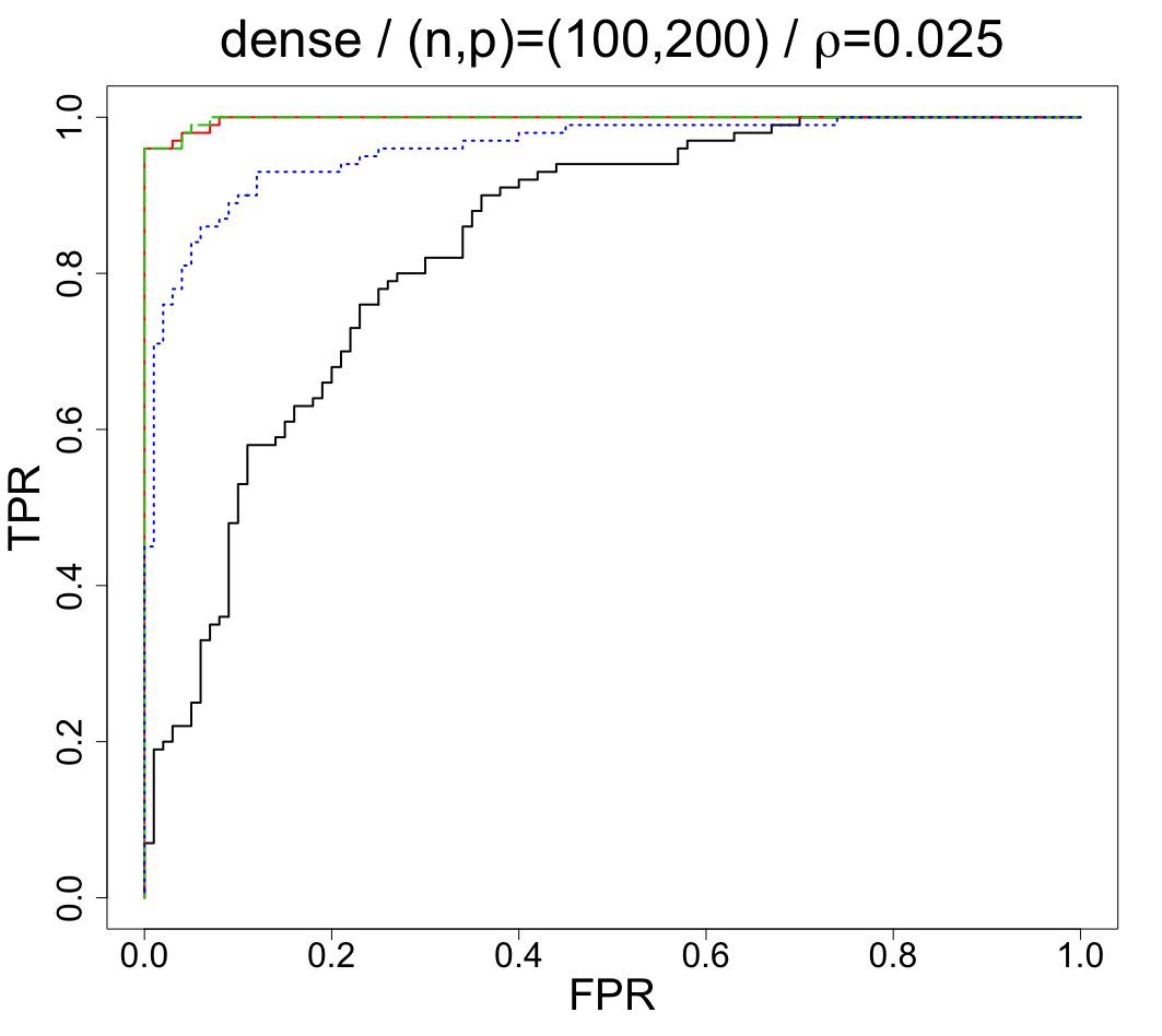
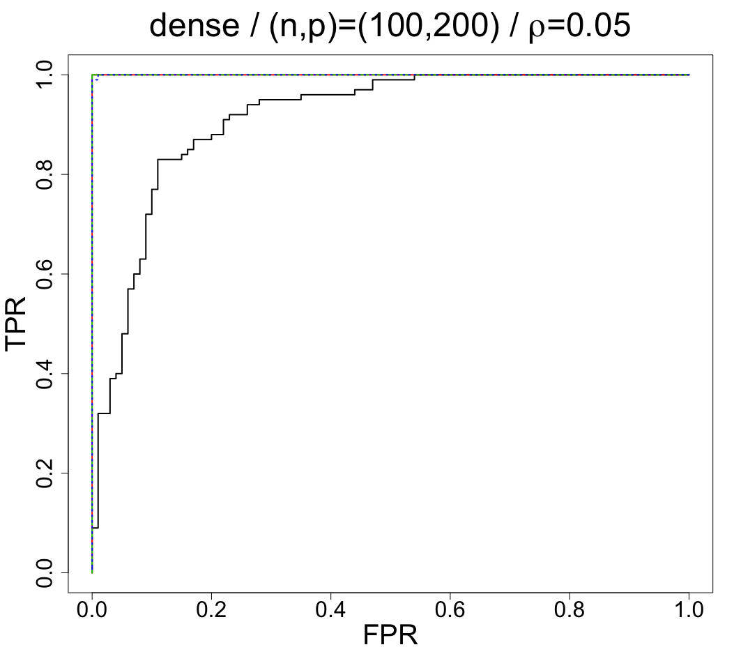
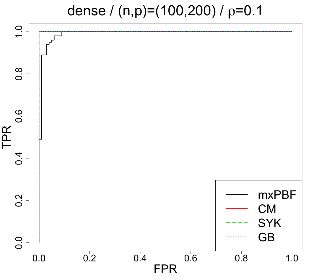
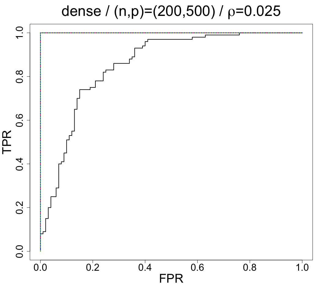
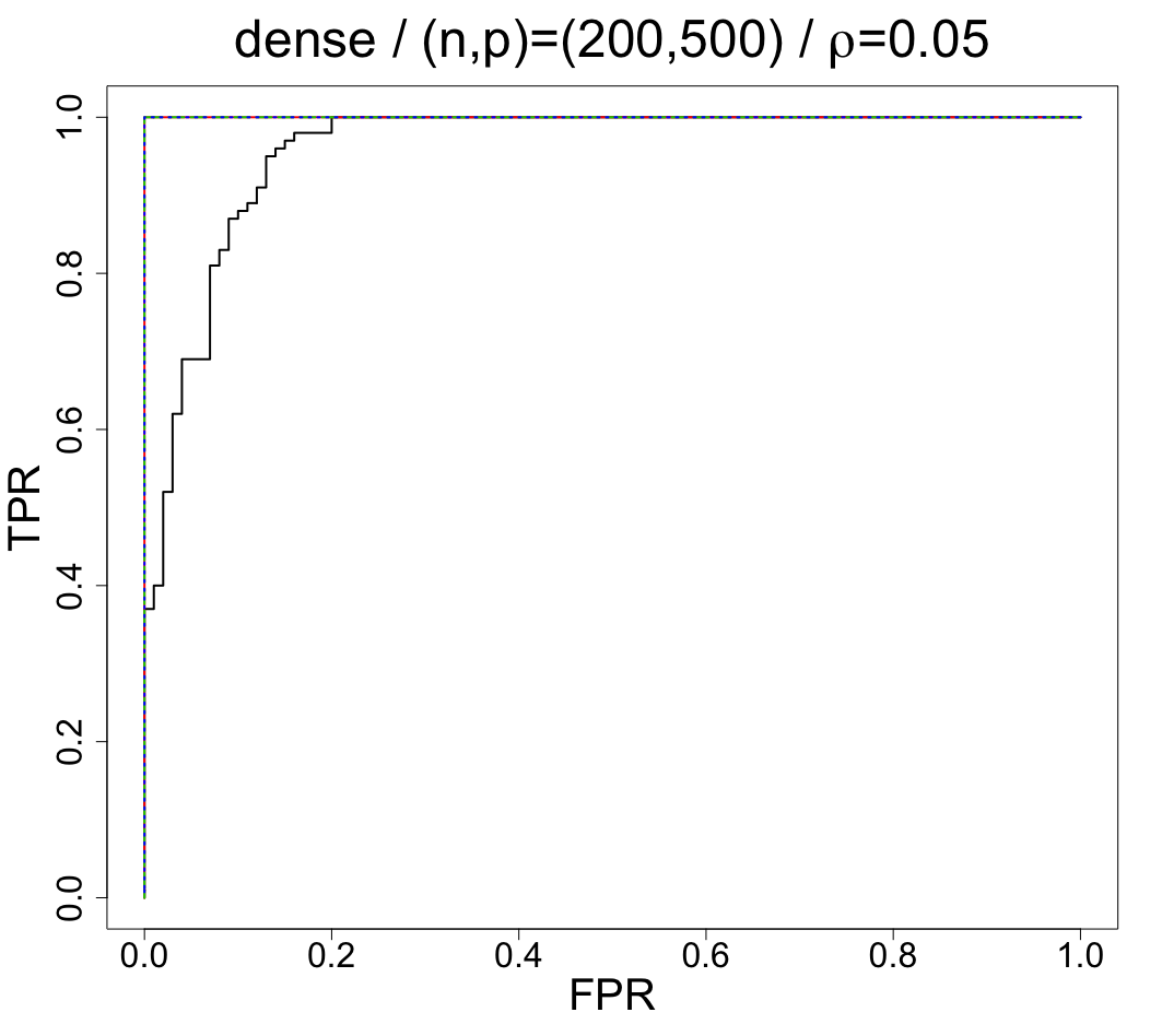
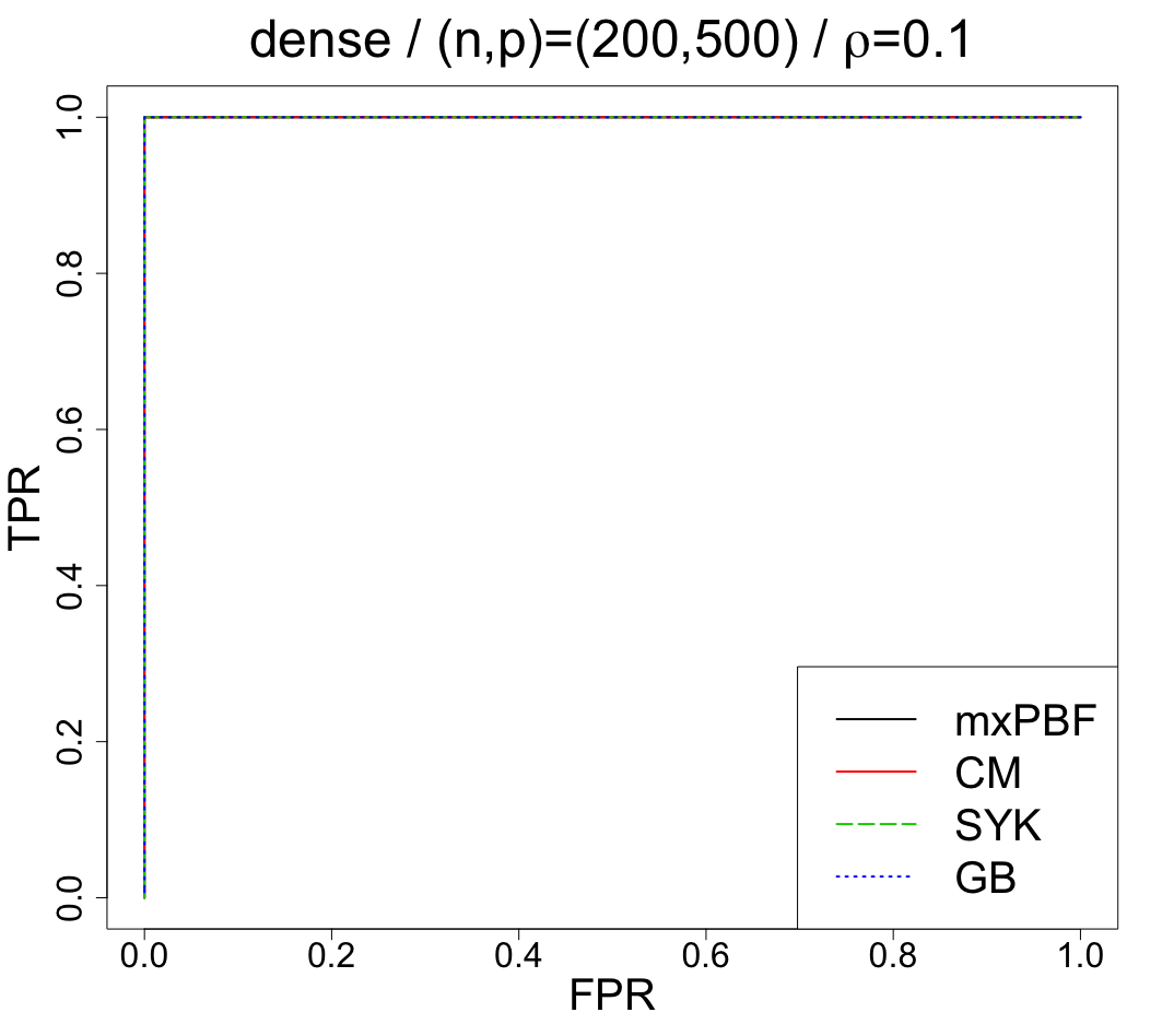
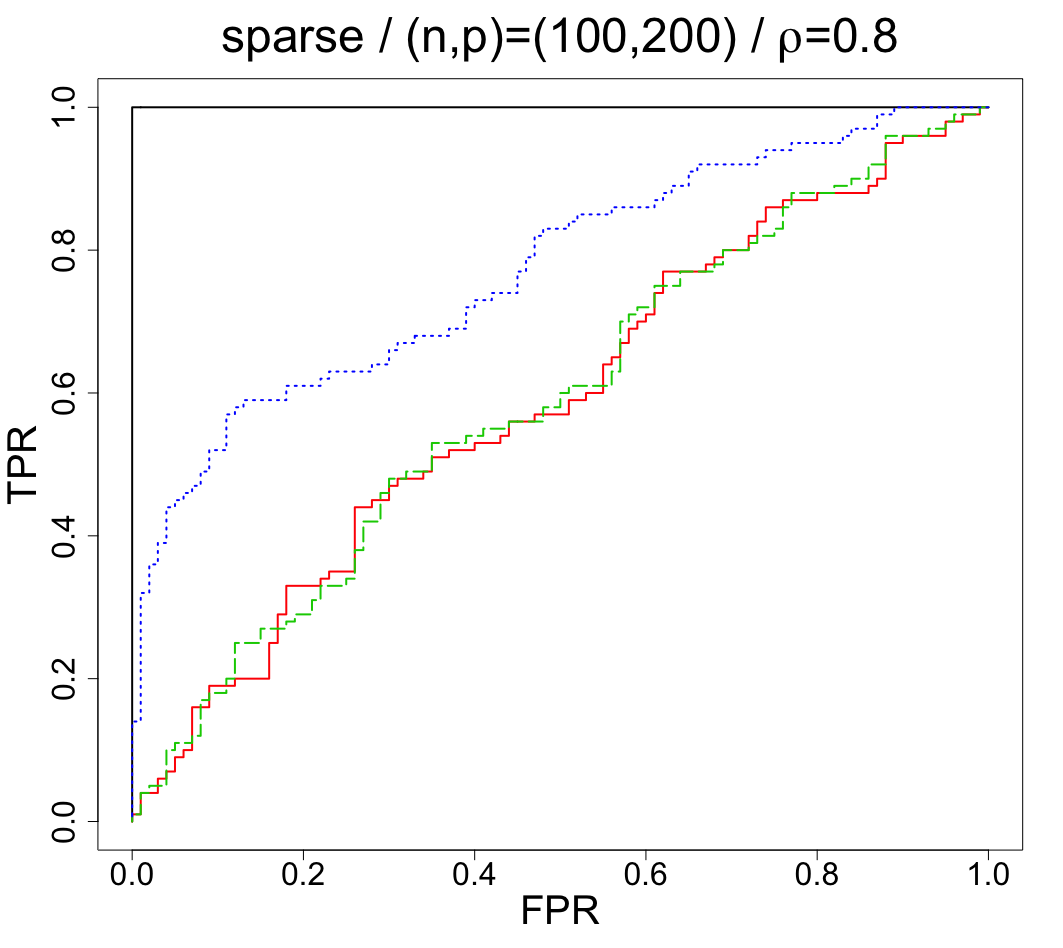
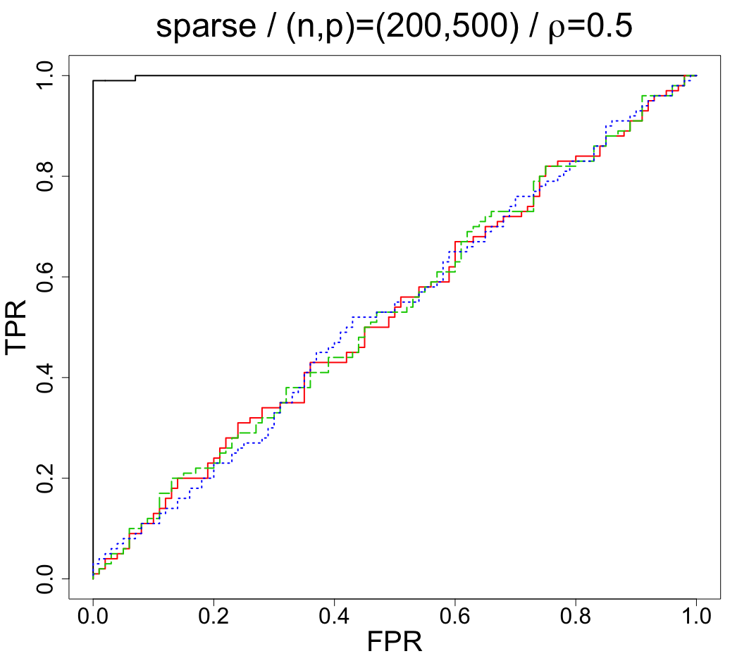
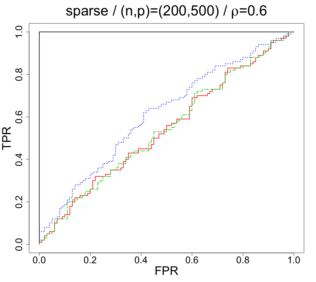
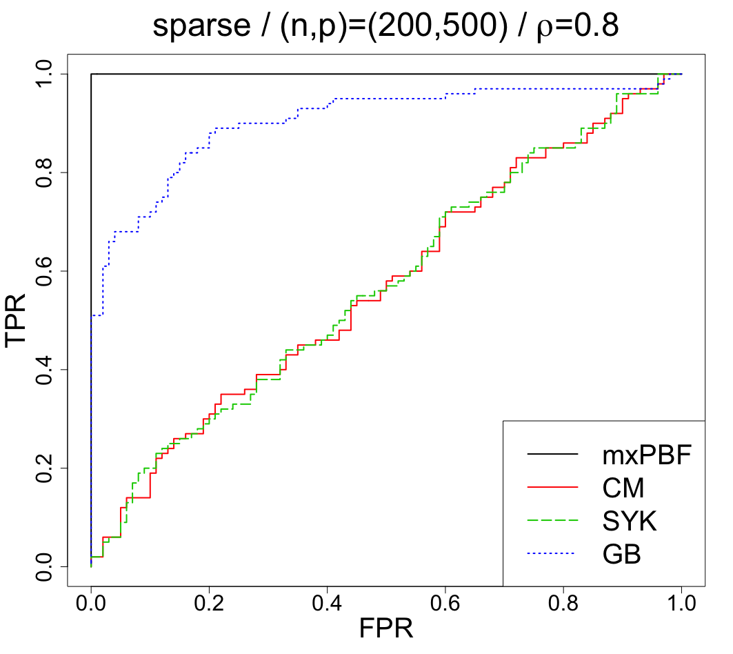
We calculated receiver operating characteristic curves to illustrate and compare the performance of the tests. For each setting, points of the curves were obtained based on various thresholds and significance levels for $B_{\max,10}(X)$ and the frequentist tests, respectively. We tried $n=100,200,300$ and $p=200,500$ for each setting. Figure 1 shows results based on 100 simulated data from $N_{p}(0,I_{p})$ ($H_{0}$) and 100 simulated data from $N_{p}(0,\Sigma_{0})$ with a compound symmetry structured $\Sigma_{0}$ ($H_{1}$) given in (15), for $(n,p)=(100,200)$ and $(n,p)=(200,500)$. The false positive rate corresponds to the rate of $H_{0}$’s falsely detected as $H_{1}$’s. Similarly, the true positive rate is the rate of $H_{1}$’s correctly detected as $H_{1}$’s. In this setting, as expected, the tests in Cai and Ma (2013), Srivastava et al. (2014) and Gupta and Bodnar (2014) work better than the test proposed in this paper. However, as we can see from the second and third columns in Figure 1, $B_{\max,10}(X)$ also performs well so long as there is a meaningful signal somewhere. The only case when our method is not as powerful is when weak signals are spread through the alternative covariance matrix, in which case one may question the meaningfulness of the signals.

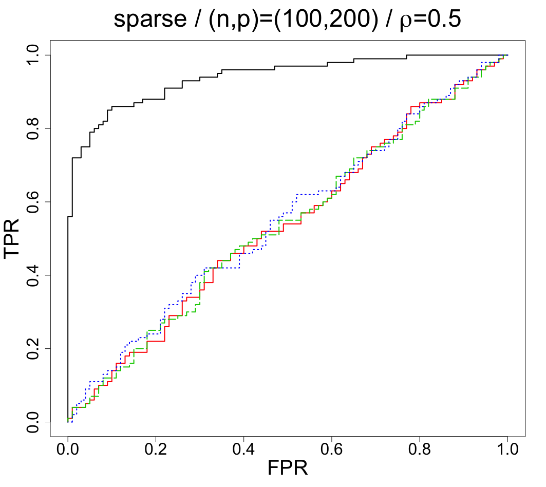
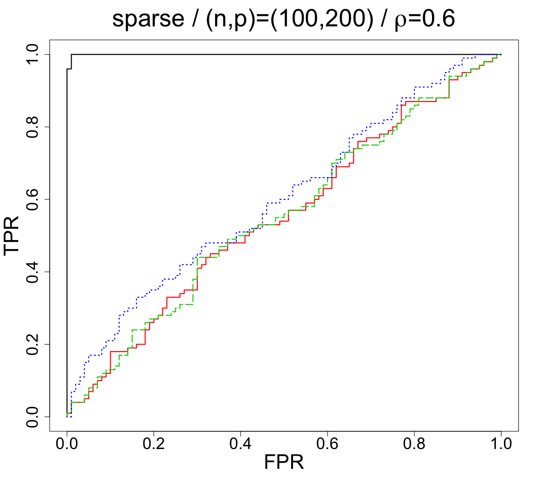
Figure 2 shows results based on 100 simulated data from $N_{p}(0,I_{p})$ and 100 simulated data from $N_{p}(0,\Sigma_{0})$ with $\Sigma_{0}$ given in (16), when $(n,p)=(100,200)$ and $(n,p)=(200,500)$. As expected, $B_{\max,10}(X)$ is much more powerful than the frequentist tests when $\Sigma_{0}-I_{p}$ is sparse. Furthermore, the performances of the frequentist tests based on the Frobenius norm are almost the same for every setting, while $B_{\max,10}(X)$ has better performance when $(n,p)=(200,500)$ than $(n,p)=(100,200)$. Interestingly, the performance of the test in Gupta and Bodnar (2014) improves as the signal strength $\rho$ increases. Thus, the test in Gupta and Bodnar (2014) is more sensitive to sparse changes than other tests based on the Frobenius norm difference. This makes sense because it focuses on the changes in a column of the covariance matrix rather than in the whole covariance matrix.

4.2 Simulation Study: Testing Diagonality

We conducted a simulation study to illustrate the performance of our proposed diagonality test. The hyperparameter $\alpha$ was chosen as $\alpha=4.01(1-1/\log n)$. We generated 100 data sets from the null $H_{0}:\sigma_{ij}=0$ for any $i\neq j$ using $\Sigma_{0}=I_{p}$. The two structures of $\Sigma_{0}$ under $H_{1}$ used in the previous section, (15) and (16), were considered. For each setting, 100 data sets were generated.

We compare our test with some existing frequentist tests. Cai and Jiang (2011) proposed a diagonality test based on the maximum of sample correlations. Here $\widehat{\tau}_{ij,\gamma}^{2}$ in the pairwise Bayes factor $\tilde{B}_{10}(\tilde{X}_{i},\tilde{X}_{j})$ is a decreasing function of the sample correlation between $\tilde{X}_{i}$ and $\tilde{X}_{j}$. Lan et al. (2015) developed a test in the regression setting based on the squared Frobenius norm of a sample covariance matrix. Their test should be powerful against dense alternatives. We also conducted maximum-type tests based on Kendall’s tau and Spearman’s rho (Han et al., 2017). Chen and Liu (2018) assumed $p$-dimensional observations from a common multivariate normal distribution and investigated the dependence among samples. Since their method can be applied to the diagonality test by considering $X^{T}$ instead of $X$, we included it as a contender. Their test requires $p=O(n)$ and the uniformly bounded condition for the eigenvalues of $\Sigma_{0}$ for theoretical properties, excluding the high-dimensional setting $p\gg n$ and some interesting covariance classes like compound symmetry. Finally, we also considered frequentist union-intersection tests based on the p-values associated with the marginal independence tests. A $t$-test for Pearson’s correlation was conducted for testing $H_{0,ij}:\sigma_{ij}=0$ for each pair $i>j$, and the null hypothesis $H_{0}:\sigma_{ij}=0$ for any $i\neq j$ was rejected if at least one $H_{0,ij}$ was rejected. To calculate the p-values, we used the cor0.test function in the GeneNet package.

Figure 3: Area under the curves are represented for the tests based on 100 simulated data sets for each hypothesis $H_{0}:\sigma_{ij}=0$ for any $i\neq j$ and $H_{1}:$ not $H_{0}$. “dense” and “sparse” mean that the true covariance matrix $\Sigma_{0}$ under $H_{1}$ were generated from (15) and (16), respectively. mxPBF, CL and Lan represent the tests proposed in this paper, Chen and Liu (2018) and Lan et al. (2015), respectively. HCL1 and HCL2 represent the test based on Kendall’s tau and Spearman’s rho, respectively. “multiple” means the frequentist union-intersection test.

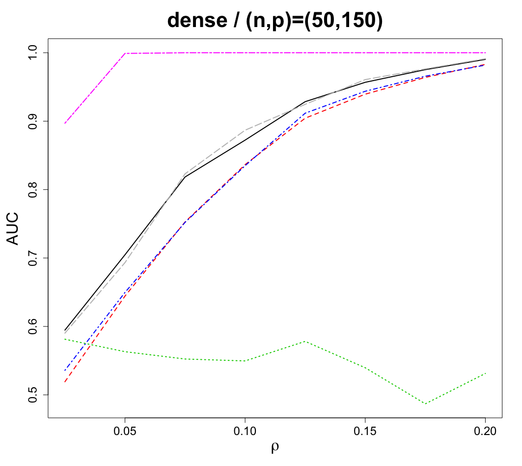
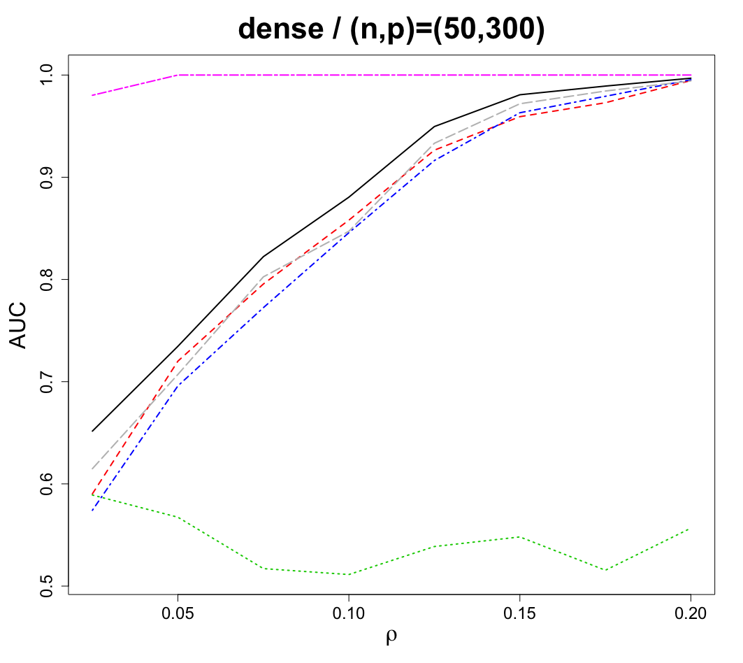
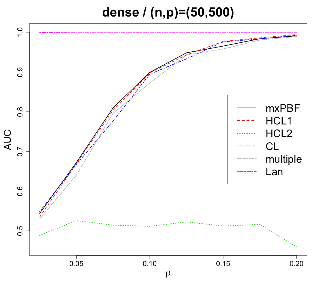
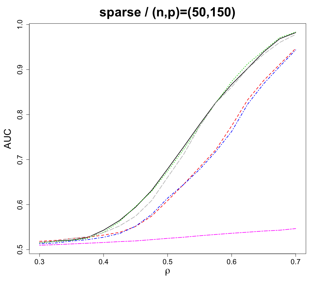
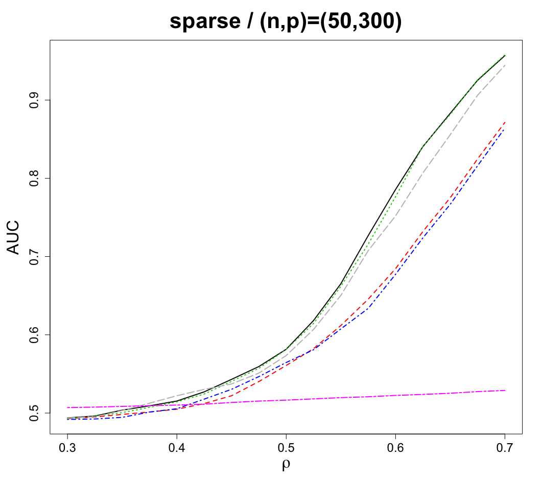
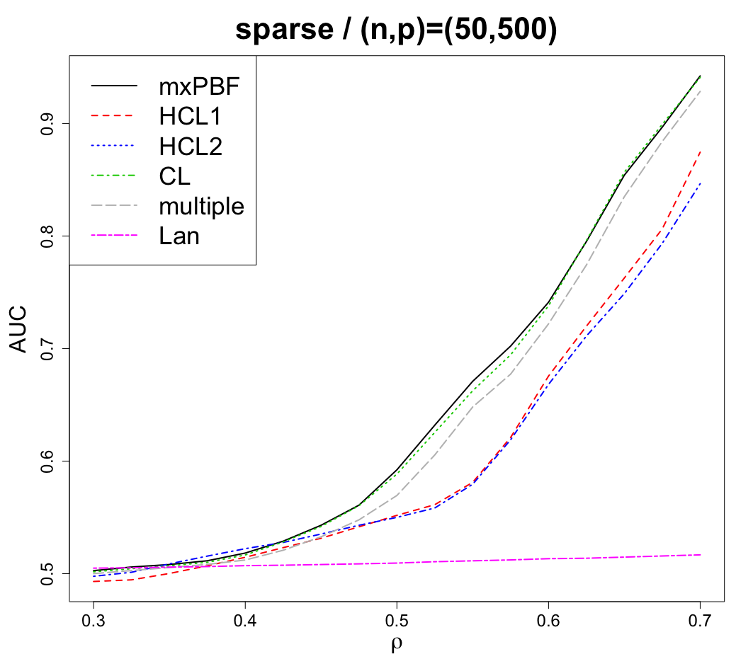
Figure 3 shows the area under the receiver operating characteristic curve for varying signal strength $\rho$ for each fixed $(n,p)$. We omit the results of Cai and Jiang (2011), which were almost identical to our test in every setting. As expected, the test of Lan et al. (2015) is more powerful against dense alternatives. The other tests, except the test of Chen and Liu (2018), have less power, but work reasonably well as the signal $\rho$ grows. The test of Chen and Liu (2018) does not work well, likely because (15) violates their assumptions. When $\Sigma_{0}-I_{p}$ is sparse, the test of Lan et al. (2015) does not work well even when $\rho$ is large. The other tests show good results against sparse alternatives, but our test has better performance.

4.3 Support Recovery using Gene Expression Data

To describe the practical performance of the support recovery procedure (14), $\widehat{S}_{pair}$, we analyzed a data set from a small round blue-cell tumor microarray experiment (Khan et al., 2001). The data set originally had 6,567 gene expression values, and 2,308 gene expressions were selected by an initial filtering (Khan et al., 2001). For comparison purposes, we focus on the preprocessed data used in Rothman et al. (2009) and Cai and Liu (2011), consisting of $p=200$ gene expression values for each of $n=64$ training tissue samples. There are four types of tumors represented in these tissue samples. Data were centered prior to analysis.

For pairwise Bayes factors, the hyperparameter was set at $\alpha=4.01(1-1/\log n)$. We used cross-validation to select $C_{sel}$. Let $n$ be the number of observations for a given data set. We randomly divided the data 50 times into two subsamples with size $n_{1}=\lceil n/3\rceil$ and $n_{2}=n-n_{1}$ as a test set and training set, respectively. Denote $I_{1}$ and $I_{2}$ as indices for the test set and training set, respectively, thus, $|I_{1}|=n_{1}$, $|I_{2}|=n_{2}$ and $I_{1}\cup I_{2}=\{1,\ldots,n\}$. Let $\hat{S}_{j}(C_{sel})$ be the estimated support for the $j$th column of the covariance matrix via pairwise Bayes factors, based on $\{X_{i}\}_{i\in I_{2}}$ and a given threshold $C_{sel}$. We calculated the averaged mean squared error

$$MSE(C_{sel}) = \sum_{j=1}^{p}\sum_{l\in\hat{S}_{j}(C_{sel})}\Big{\{}\sum_{i\in I_{1}}(X_{ij}-X_{il}\widehat{\beta}_{jl})^{2}/(n_{1}-1)\Big{\}}/|\hat{S}_{j}(C_{sel})|,$$

where $\widehat{\beta}_{jl}$ is a least square estimate with respect to the dependent variable $\{X_{ij}\}_{i\in I_{1}}$ and covariate $\{X_{il}\}_{i\in I_{1}}$. The threshold $C_{sel}$ was varied from $-7$ to $10$ with increment $0.2$, and we selected $\widehat{C}_{sel}$ which minimizes $50^{-1}\sum_{\nu=1}^{50}MSE_{\nu}(C_{sel})$, where $MSE_{\nu}(C_{sel})$ is the averaged mean squared error based on the $\nu$th split.

We compared our method with generalized thresholding estimators of Rothman et al. (2009) and Cai and Liu (2011). Rothman et al. (2009) used a universal threshold $\lambda=\delta(\log p/n)^{1/2}$, while Cai and Liu (2011) used an individual threshold $\hat{\lambda}_{ij}=\delta(\hat{\theta}_{ij}\log p/n)^{1/2}$ with a data-dependent $\hat{\theta}_{ij}$. We denote thresholding estimators proposed by Rothman et al. (2009) and Cai and Liu (2011) by $\widehat{\Sigma}_{\delta}$ and $\widehat{\Sigma}_{\delta}^{\star}$, respectively. We used the adaptive lasso thresholding rule, $s_{\lambda}(\sigma)=\sigma\max(1-|\lambda/\sigma|^{\eta},0)$ with $\eta=4$, because it gave good support recovery results in simulation studies in Rothman et al. (2009) and Cai and Liu (2011). We adopted the cross-validation method described in Section 4 of Cai and Liu (2011) to select $\delta$ and denote the selected tuning parameter by $\hat{\delta}$.

Figure 4: The absolute sample correlation matrix (top left) and estimated supports from various methods. Clockwise from the top right are plots for the estimated supports based on $\widehat{S}_{pair,\widehat{C}_{sel}}$, $\widehat{\Sigma}_{\hat{\delta}}^{\star}$ and $\widehat{\Sigma}_{\hat{\delta}}$, respectively.

Figure 5: The ordered absolute sample correlation matrix and estimated supports for top 40 genes, with 1’s representing the estimated supports from $\widehat{S}_{pair,\widehat{C}_{sel}}$ (left) and $\widehat{\Sigma}_{\hat{\delta}}^{\star}$ (right).

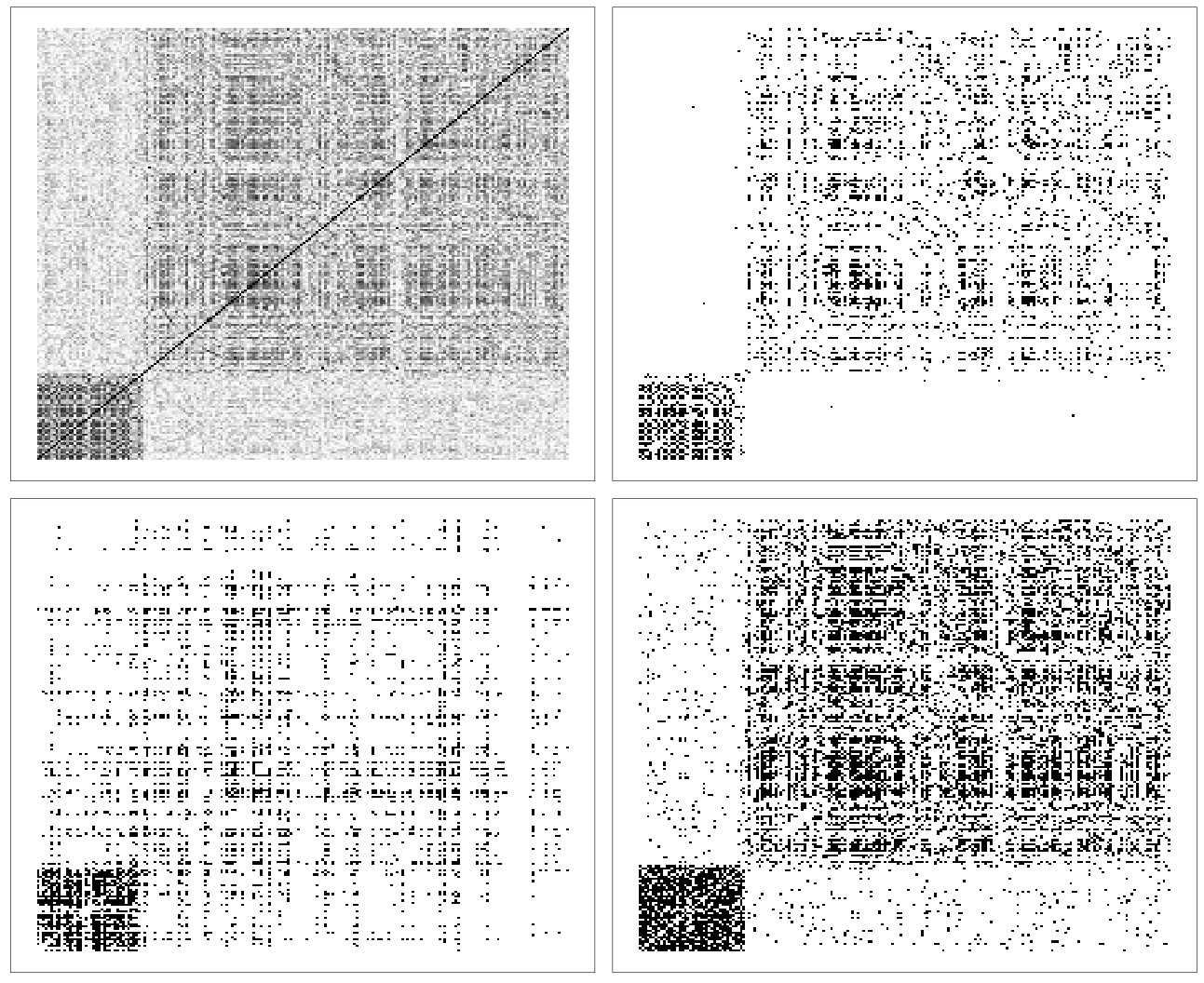
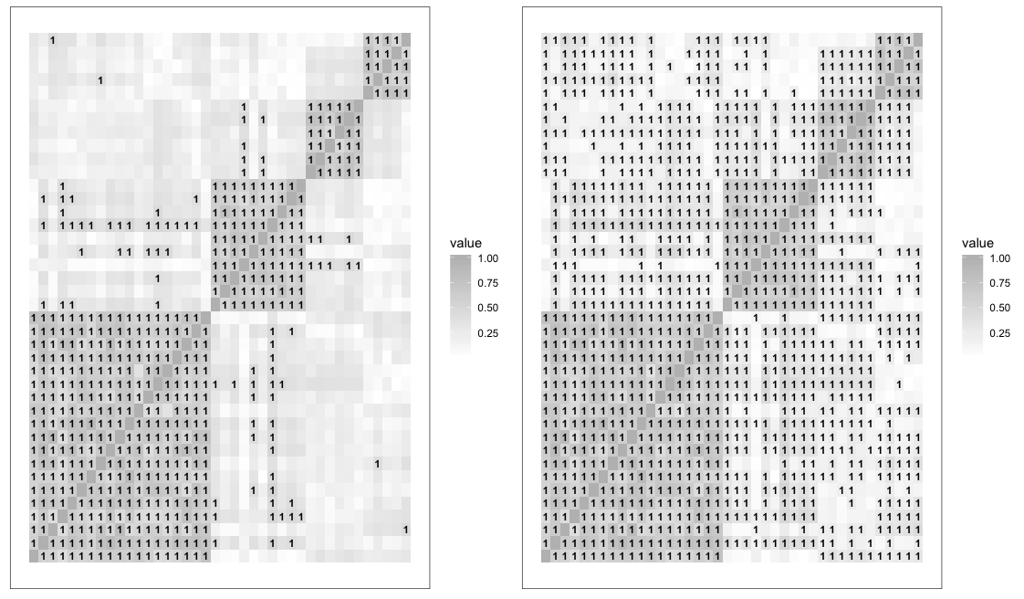
Figure 4 shows the support recovery results and the absolute sample correlation matrix. The estimated supports based on $\widehat{S}_{pair,\widehat{C}_{sel}}$, $\widehat{\Sigma}_{\hat{\delta}}^{\star}$ and $\widehat{\Sigma}_{\hat{\delta}}$ are represented. One can see that $\widehat{S}_{pair,\widehat{C}_{sel}}$ and $\widehat{\Sigma}_{\hat{\delta}}^{\star}$ show the clustering structure between informative (top 40) and non-informative (bottom 160) genes, while the structure is somewhat blurred in $\widehat{\Sigma}_{\hat{\delta}}$. To compare $\widehat{S}_{pair,\widehat{C}_{sel}}$ and $\widehat{\Sigma}_{\hat{\delta}}^{\star}$ in more detail, we further focused on the top 40 genes. We applied hierarchical clustering to the genes based on the complete linkage method using R function hclust, and the genes were ordered according to the clustering result. Figure 5 shows the ordered absolute sample correlation matrix and estimated supports for the top 40 genes. The clustering result suggests that there are four clusters, consistent with the four tumor types. Both support recovery procedures detect significant blocks in the sample correlation matrix. However, our support recovery procedure shows the clustering structure much clearer, while $\widehat{\Sigma}_{\hat{\delta}}^{\star}$ gives a blurred structure due to a dense support estimate. The estimated support based on pairwise Bayes factors has the advantage of producing a sparser, and hence potentially more interpretable, estimate of support.

5 Discussion

We have focused on covariance matrix structure testing in this paper, but the maximum pairwise Bayes factor idea can be easily applied to other related settings. For example, testing differences across groups in high-dimensional mean vectors is an interesting possibility. When the two mean vectors are almost the same but differ only at a few locations, a maximum pairwise Bayes factor approach should have relatively high power. Similarly, it can be applied to the high-dimensional two-sample covariance test. Two covariances from two populations may differ only in a small number of entries.

There are some possible generalizations of the pairwise Bayes factor idea. To accelerate the speed of computation, a random subsampling method can be used instead of calculating the pairwise Bayes factor for every single pair $(i,j)$. It should be interesting to develop a suitable random subsampling or random projection scheme achieving desirable theoretical properties. Especially when $p$ is huge, it will effectively reduce the computational complexity. The maximum pairwise Bayes factor approach is also trivially parallelizable. Another possibility is considering alternative combining approaches to the max in merging the information from every pairwise Bayes factor. If there are many weak non-zero covariances, then the average or summation may be preferable to the maximum. A suitable modification to learn parameters in the combining operator can potentially make the test powerful to a broad class of alternative hypotheses.

Appendix A Testing pairwise independence

As a by-product of Theorem 3, when pairwise independence testing (3.12) itself is of interest, we suggest a pairwise Bayes factor $\tilde{B}_{10}(\tilde{X}_{i},\tilde{X}_{j})$, which can be shown to be consistent. For consistency under the alternative hypothesis, we assume

$$\sigma_{0,ij}^{2} \geq \frac{C_{4}\sigma_{0,jj}}{1-2\epsilon_{0}{C_{1}}^{1/2}}\left\{\frac{9C_{1}\tau_{0,ij}^{2}}{(1-C_{3})^{2}}\vee\frac{\alpha(1+\gamma)(1+4\epsilon_{0}{C_{1}}^{1/2})\sigma_{0,ii}}{C_{3}}\right\}\frac{\log n}{n}\quad\quad\quad$$ (17)

for constants $C_{1}>0,0<C_{3}<1$ and $C_{4}>1$ defined in Section 3.1. If we substitute $\log n$ in the above condition with $\log(n\vee p)$, it coincides with condition (A4). The proof of Corollary 1 follows from that of Theorem 3, and thus it is omitted.

Corollary 1

Consider model (1.1) and a hypothesis testing problem (3.12) for a given pair $(i,j)$ such that $i\neq j$. Suppose we use the prior $\pi(\tau_{ij}^{2})\propto\tau_{ij}^{-2}$ under both $H_{0,ij}$ and $H_{1,ij}$, and the prior $\pi(a_{ij}\mid\tau_{ij}^{2})$ defined in (2.5) under $H_{1,ij}$ with $\gamma=n^{-\alpha}$ for some positive constant $\alpha$. Then under $H_{0,ij}:\sigma_{ij}=0$, for some constant $c>0$,

$$\tilde{B}_{10}(\tilde{X}_{i},\tilde{X}_{j}) = O_{p}\big{(}n^{-c}\big{)}.$$

If, under $H_{1,ij}:\sigma_{ij}\neq 0$, at least one of $\sigma_{0,ij}$ and $\sigma_{0,ji}$ satisfies (17), for some constant $c^{\prime}>0$,

$$\tilde{B}_{10}(\tilde{X}_{i},\tilde{X}_{j})^{-1} = O_{p}\big{(}n^{-c^{\prime}}\big{)}.$$

Appendix B Simulation Study: Support Recovery

The proposed support recovery procedure, $\widehat{S}_{pair,C_{sel}}$, consistently recovers the true support $S(\Sigma_{0})$ for any constant threshold $C_{sel}$ (Theorem 4). However, in practice, the choice of the threshold is crucial. In this section, we investigate the quality of $\widehat{S}_{pair,C_{sel}}$ as a function of the threshold $C_{sel}$ to assess the importance of the choice of $C_{sel}$. Furthermore, the performance of the cross-validation-based threshold $\widehat{C}_{sel}$ proposed in Section 4.3 also will be demonstrated.

Two structures of covariance matrices were investigated. In the first setting, we consider

$$\sigma_{0,ij}^{*} = 2\max\Big{(}1-\frac{|i-j|}{10},\,0\Big{)}I\left\{|i-j|\leq 5,\,(i\vee j)\leq\frac{p}{2}\right\}$$

for $i\neq j$. In the second setting, we consider

$$\sigma_{0,ij}^{*} = 2\max\Big{(}1-\frac{|i-j|}{10},\,0\Big{)}I\left\{|i-j|\leq 5,\,i\leq\frac{p}{2}\right\}$$

$$+\,\,2\max\Big{(}1-\frac{|i-j|}{20},\,0\Big{)}I\left\{|i-j|\leq 10,\,i>\frac{p}{2}\right\}$$

for $i<j$. In both settings, we set $\sigma_{0,ii}^{*}=1$ and $\sigma_{0,ij}^{*}=\sigma_{0,ji}^{*}$, where $\Sigma_{0}^{*}=(\sigma_{0,ij}^{*})$. Let $\Sigma_{0}=(\sigma_{0,ij})$ be the true covariance matrix. If $\Sigma_{0}^{*}$ is positive definite, $\Sigma_{0}=\Sigma_{0}^{*}$ is used, and if $\Sigma_{0}^{*}$ is not positive definite, $\Sigma_{0}=(\sigma_{0,ij})$ is used where $\sigma_{0,ij}=\sigma_{0,ij}^{*}$ and $\Sigma_{0,ii}=\Sigma_{0,ii}^{*}-\lambda_{\min}(\Sigma_{0})+0.01$ for all $1\leq i\neq j\leq p$. The data were generated from $N_{p}(0,\Sigma_{0})$ with $n=50,100$ and $p=100,300$. To illustrate the performance of the estimated support $\widehat{S}_{pair,C_{sel}}$, we consider (i) the Matthews correlation coefficient,

$$MCC = \frac{TP\times TN-FP\times FN}{\{(TP+FP)(TP+FN)(TN+FP)(TN+FN)\}^{1/2}},$$

and (ii) the number of errors, $FP+FN$, where $TP,TN,FP$ and $FN$ are true positive, true negative, false positive and false negative, respectively.

Figure 6: MCC (Matthews correlation coefficient) and the number of errors for the first setting. The red vertical line is the cross-validation-based threshold $\widehat{C}_{sel}$.

Figure 7: MCC (Matthews correlation coefficient) and the number of errors for the second setting. The red vertical line is the cross-validation-based threshold $\widehat{C}_{sel}$.

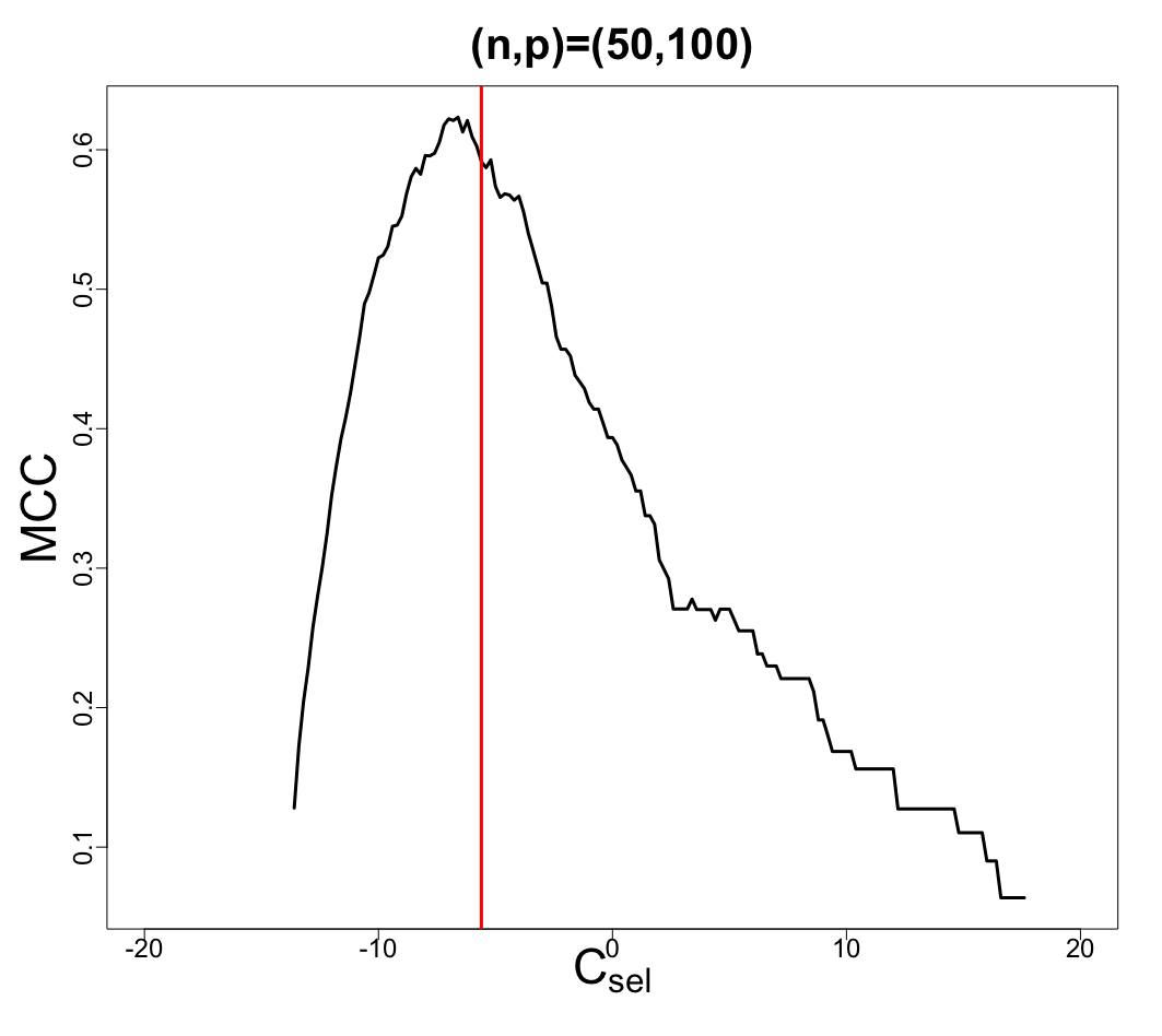
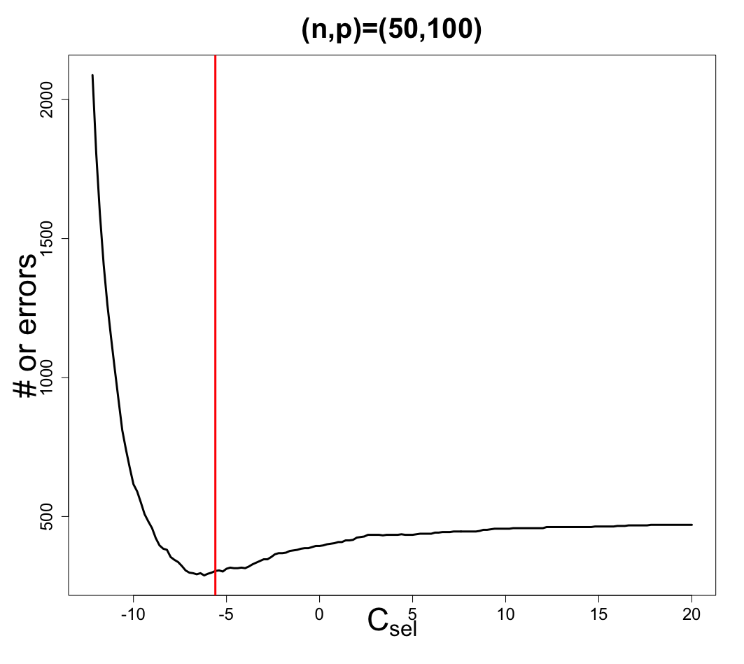
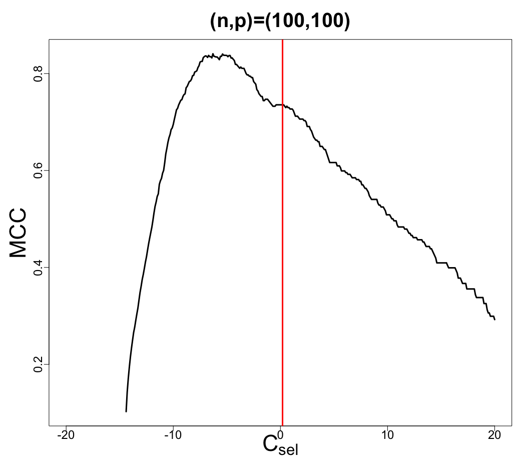
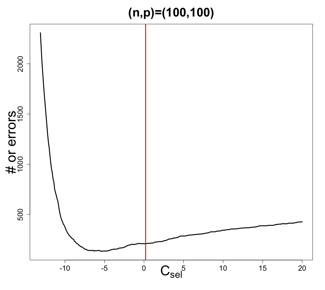
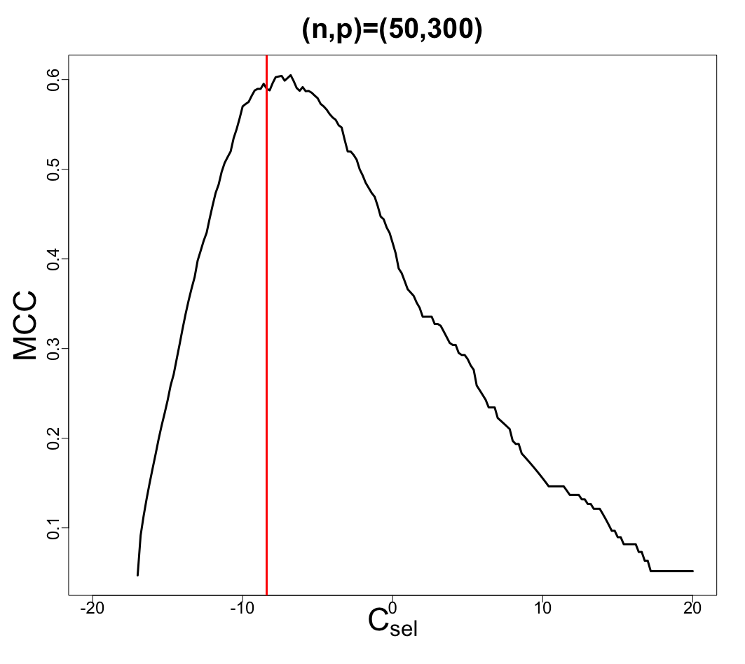
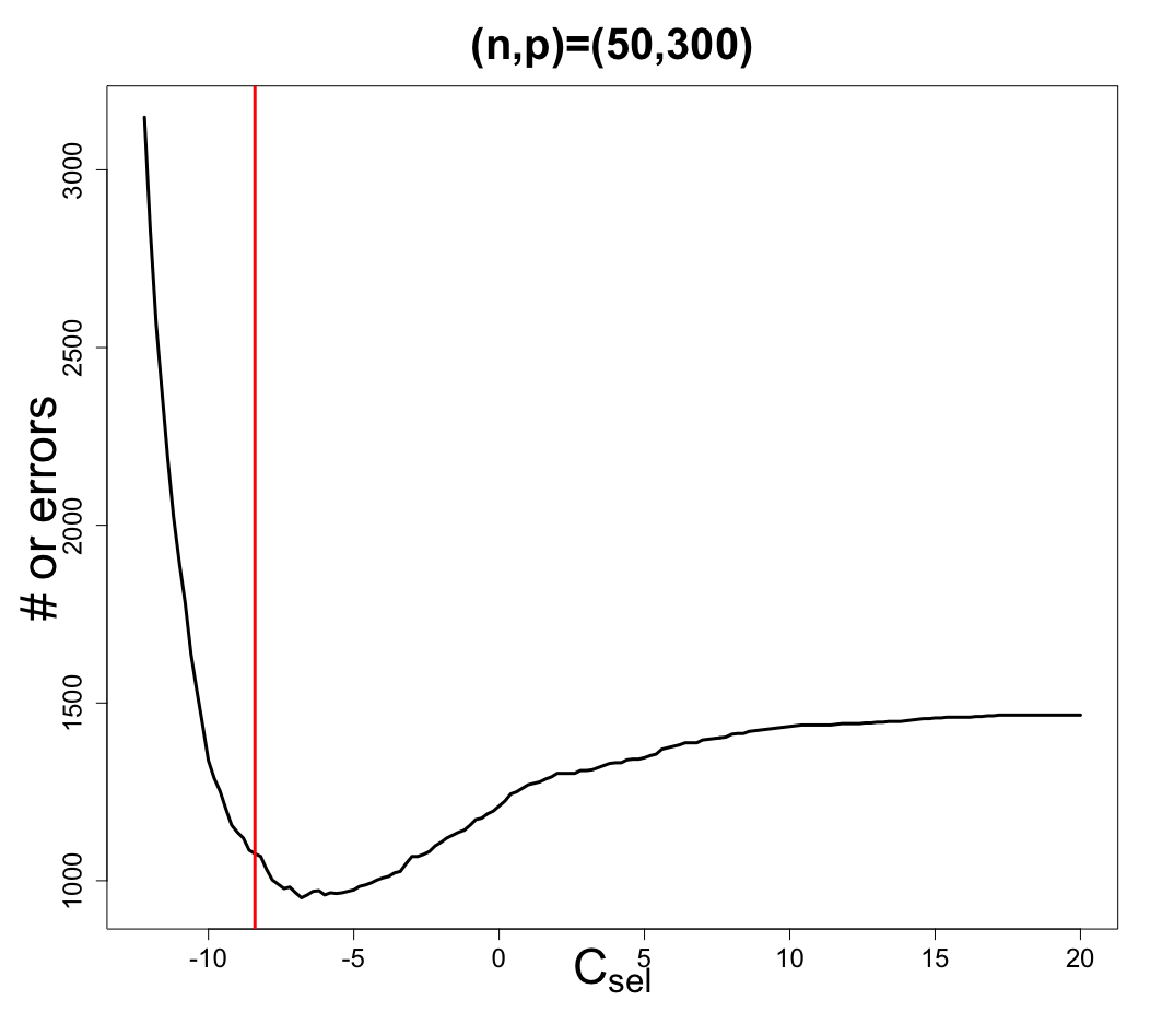
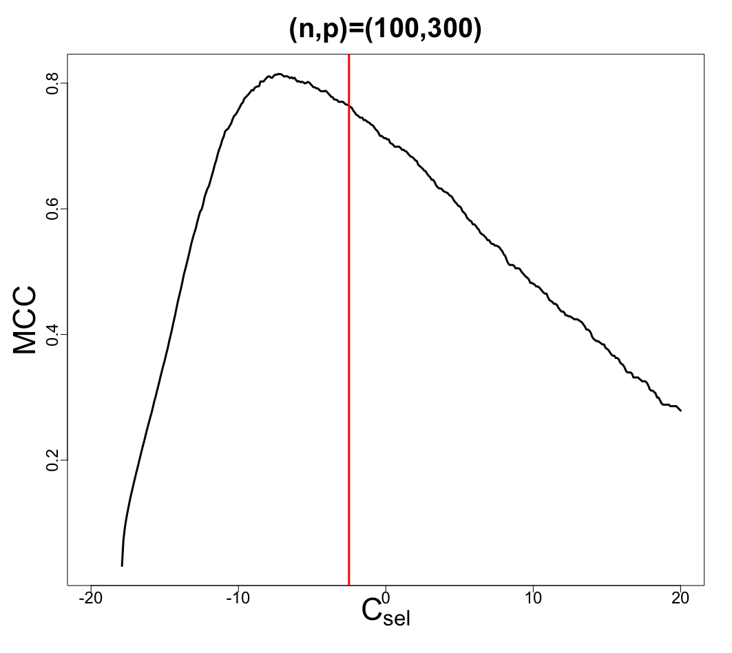
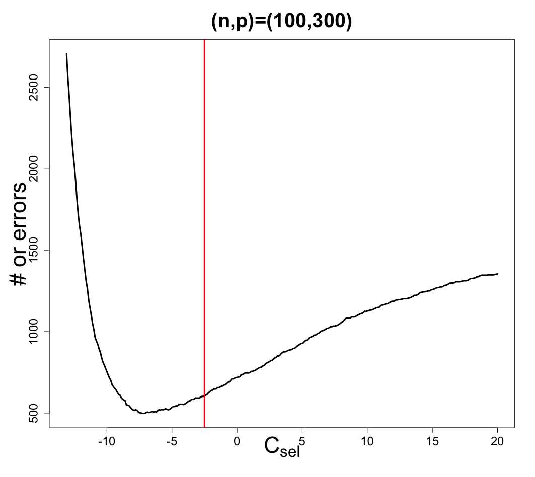
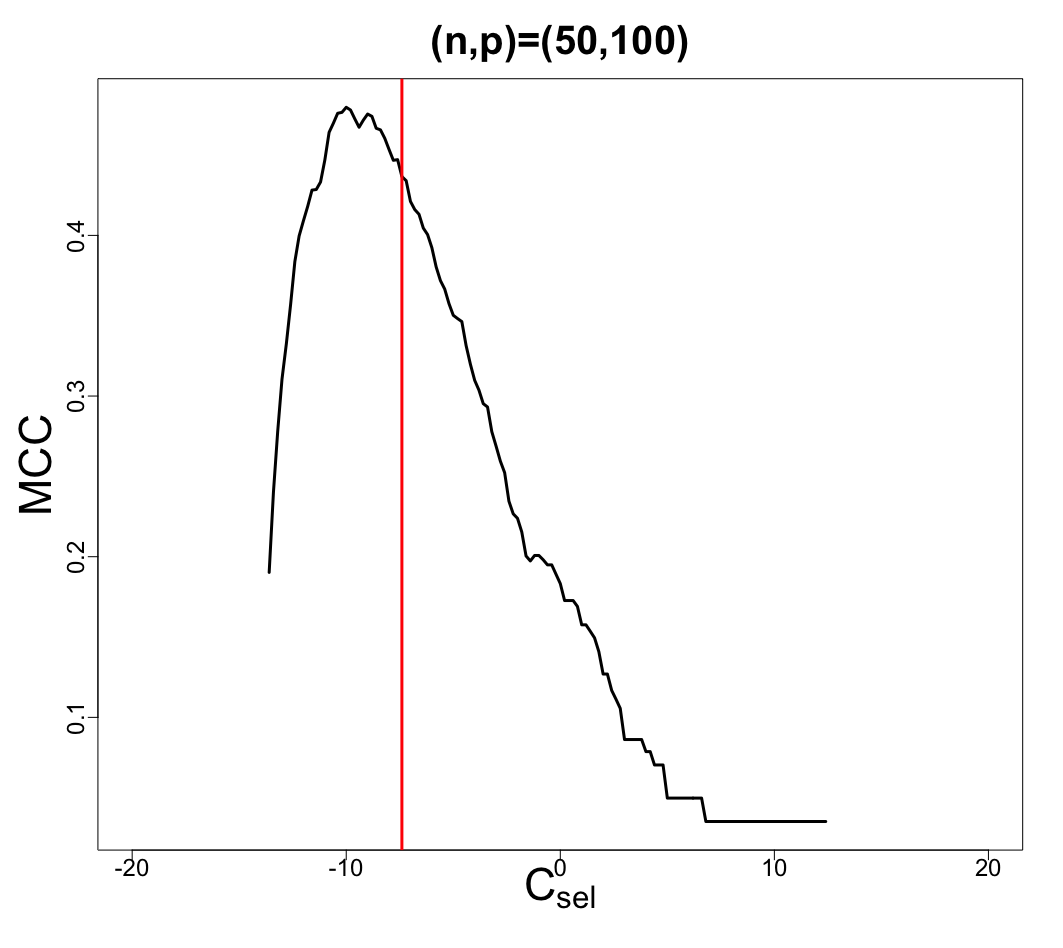
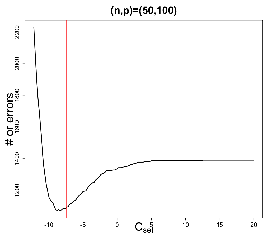
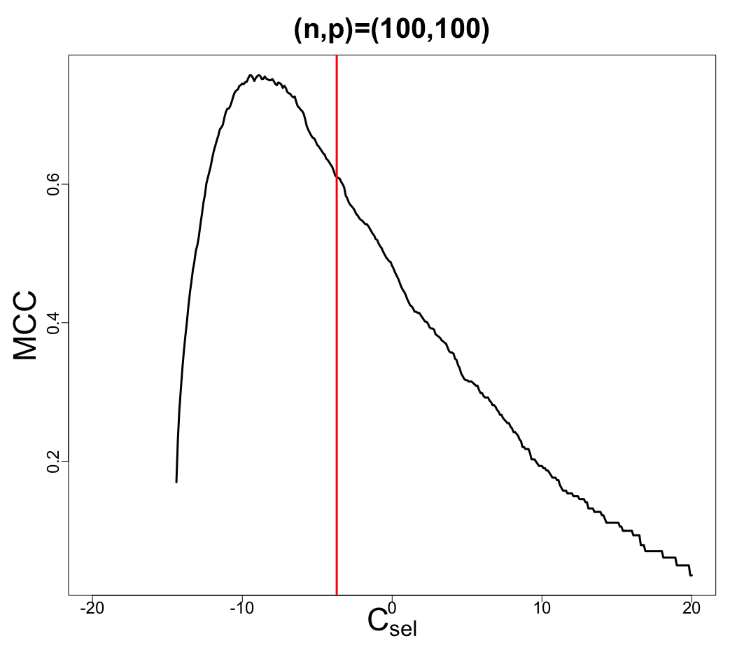
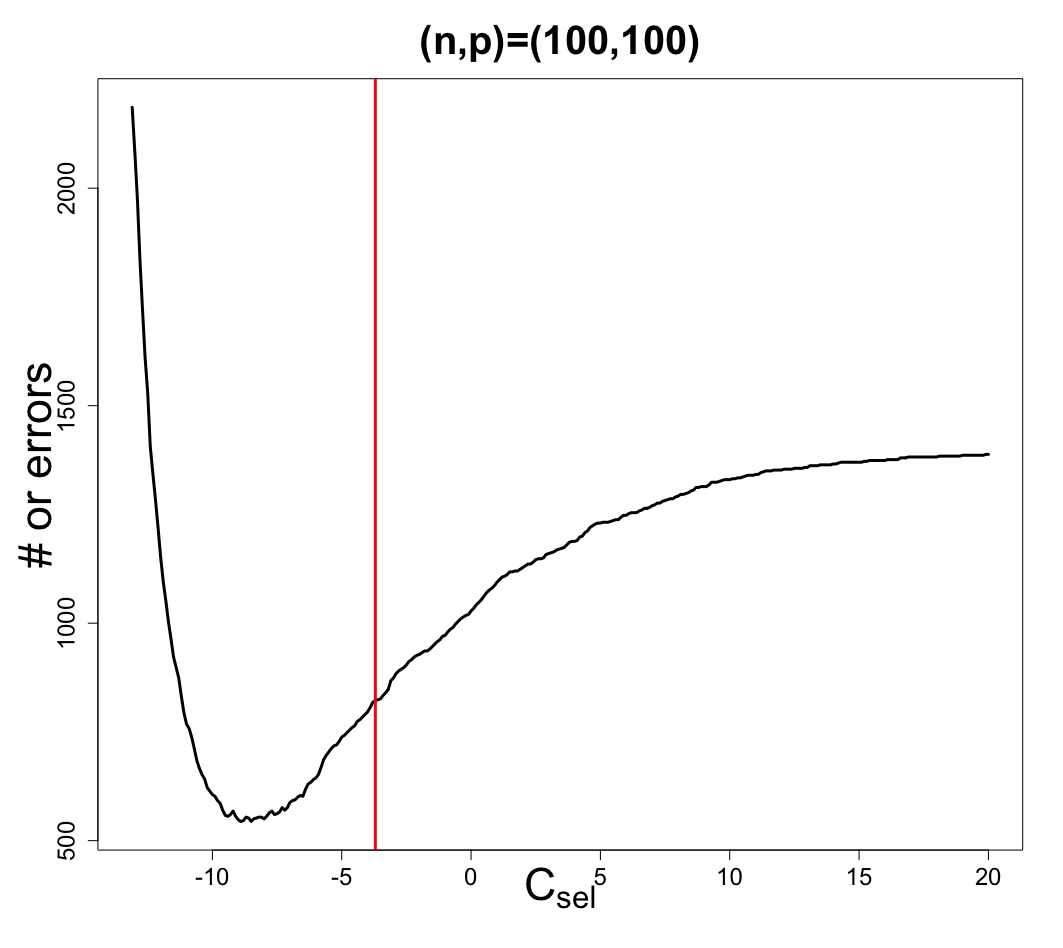
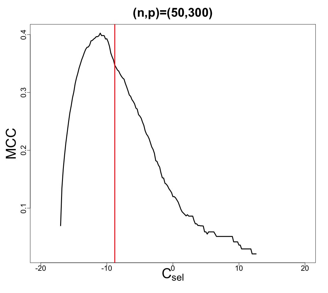
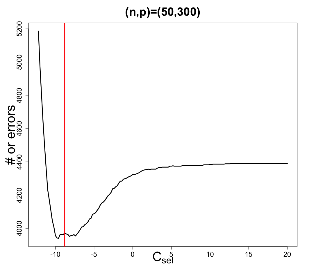
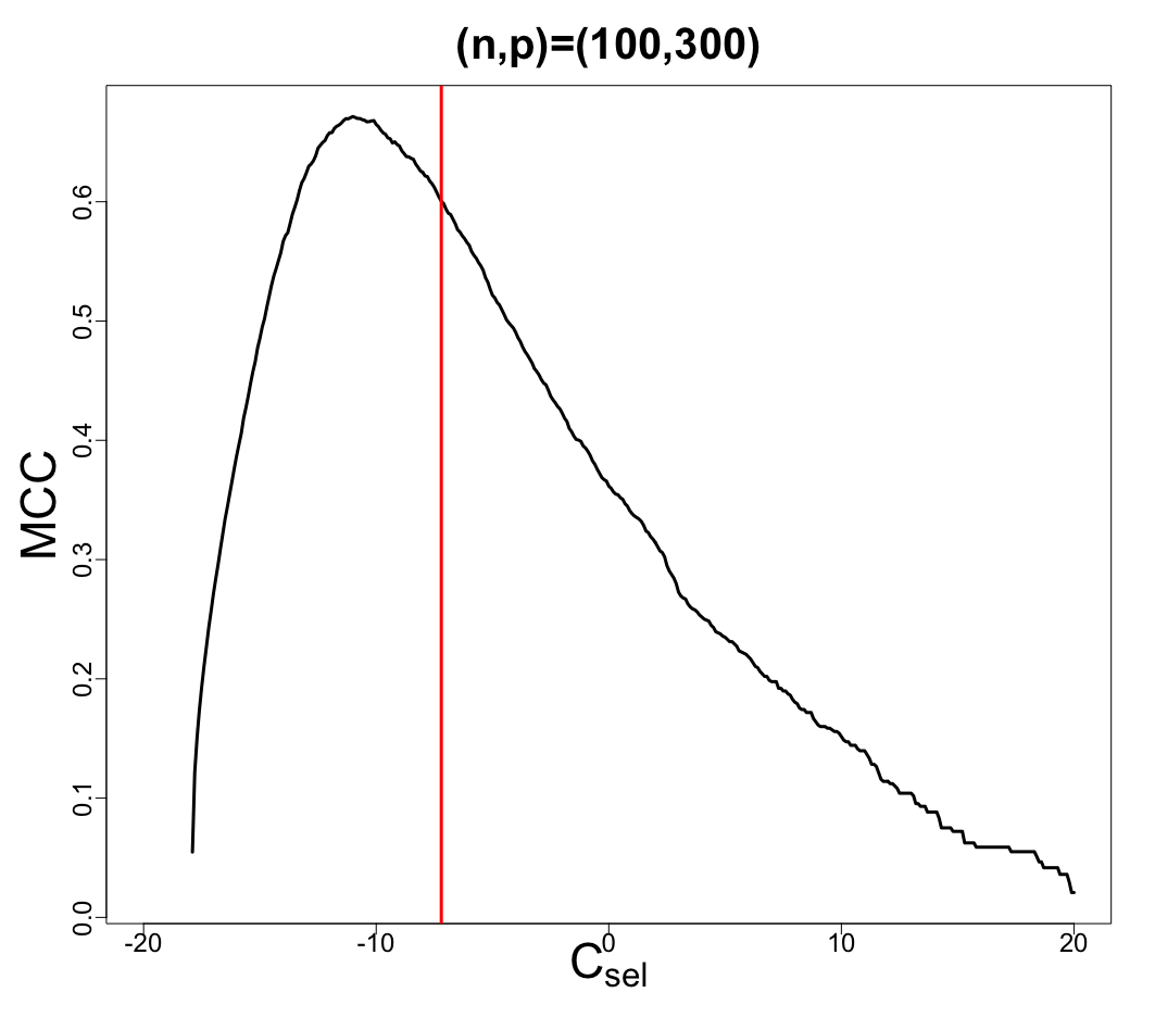
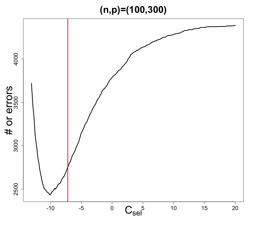
Figures 6 and 7 show the performance of $\widehat{S}_{pair,C_{sel}}$ for the first setting and the second setting, respectively. Each plot represents the performance of $\widehat{S}_{pair,C_{sel}}$ as a function of the threshold $C_{sel}$, where the red vertical line is the cross-validation-based threshold $\widehat{C}_{sel}$. We found that the quality of a fixed threshold changes with the sample size $n$, the dimension $p$ and the structure of $\Sigma_{0}$. The estimated $\widehat{C}_{sel}$ has reasonable performance in terms of the two criteria. Therefore, based on the simulation results, the cross-validation-based threshold $\widehat{C}_{sel}$ seems adequate for adaptive selection of the threshold.

Figure 8: The character $1$ indicates the estimated supports based on $\widehat{C}_{sel}$ for the first setting with $p=300$ when $n=50$ (left) and $n=100$ (right). The values in red represent the entries of the true covariance matrix.

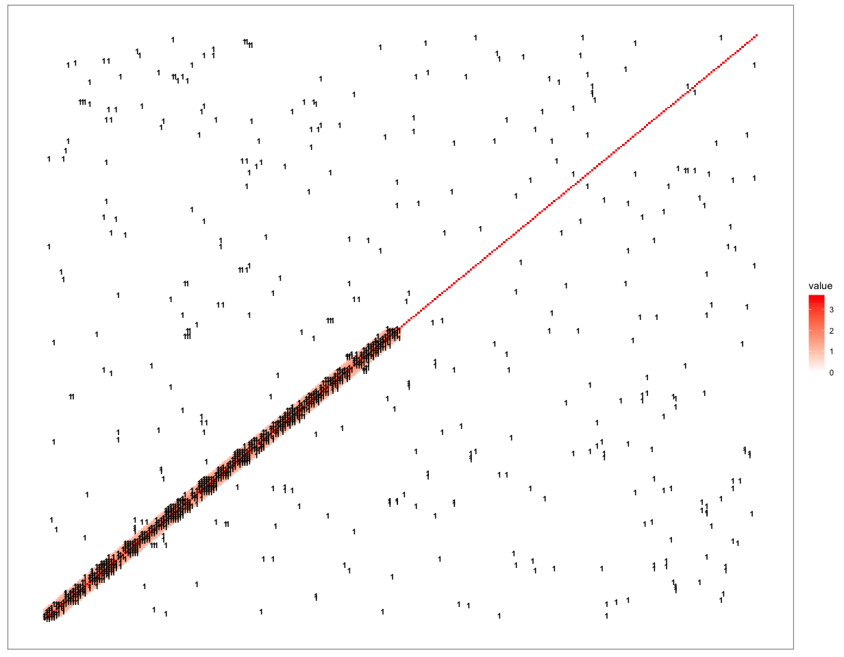
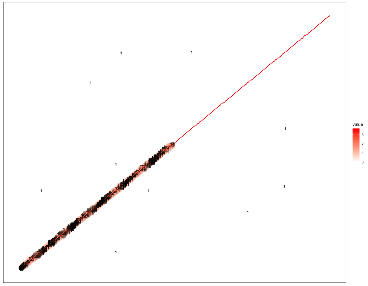
Figure 8 represents the estimated support $\widehat{S}_{pair,\widehat{C}_{sel}}$ for the first setting with $p=300$. It shows that the cross-validation-based threshold $\widehat{C}_{sel}$ has reasonable performance and the quality of the support recovery increases as the sample size gets larger.

Appendix C Proof of Theorem 1

• For a given pair $(i,j)$,

  $$\log B_{10}(\tilde{X}_{i},\tilde{X}_{j})$$ (18)

  $$= a_{0}\log b_{0,ij}+\frac{1}{2}\log\Big{(}\frac{\gamma}{1+\gamma}\Big{)}$$

  $$+ \Big{\{}\log\Gamma\big{(}\frac{n}{2}+a_{0}\big{)}-\log\Gamma(a_{0})-\big{(}\frac{n}{2}+a_{0}\big{)}\log\frac{n}{2}+\frac{n}{2}\Big{\}}$$ (19)

  $$+ \Big{\{}\frac{n}{2}\widehat{\tau}_{i}^{2}-\big{(}\frac{n}{2}+a_{0}\big{)}\log\big{(}\widehat{\tau}_{ij,\gamma}^{2}+\frac{2b_{0,ij}}{n}\big{)}-\frac{n}{2}\Big{\}}.$$ (20)

  Equation (19) can be written as

  $$\log\Gamma\big{(}\frac{n}{2}+a_{0}\big{)}-\log\Gamma\big{(}1+a_{0}\big{)}+a_{0}-\big{(}\frac{n}{2}+a_{0}\big{)}\log\frac{n}{2}+\frac{n}{2},$$

  where by Theorem 1 of Keckic and Vasic (1971),

  $$\big{(}\frac{n}{2}+a_{0}-1\big{)}\log\big{(}\frac{n}{2}+a_{0}\big{)}-a_{0}\log(1+a_{0})-\frac{n}{2}+1\,\,\leq\,\,\log\Gamma\big{(}\frac{n}{2}+a_{0}\big{)}-\log\Gamma\big{(}1+a_{0}\big{)}$$

  $$\leq \big{(}\frac{n}{2}+a_{0}-\frac{1}{2}\big{)}\log\big{(}\frac{n}{2}+a_{0}\big{)}-(\frac{1}{2}+a_{0})\log(1+a_{0})-\frac{n}{2}+1.$$

  Thus, it is easy to see that (19) is equal to

  $$-C\log\Big{(}\frac{n}{2}+a_{0}\Big{)}+\Big{(}a_{0}+\frac{2a_{0}^{2}}{n}\Big{)}\log\Big{(}1+\frac{2a_{0}}{n}\Big{)}^{n/2a_{0}}+C^{\prime}$$ (21)

  for some constants $1/2<C<1$ and $a_{0}\{1-\log(1+a_{0})\}+1-0.5\log(1+a_{0})<C^{\prime}<a_{0}\{1-\log(1+a_{0})\}+1$, which is of order $O(-\log n)$. Since $\gamma=(n\vee p)^{-\alpha}$, (18) is equal to

  $$a_{0}\log b_{0,ij}-\frac{\alpha}{2}\log(n\vee p)-\frac{1}{2}\log\big{\{}1+(n\vee p)^{-\alpha}\big{\}}$$ (22)

  $$= -\frac{\alpha}{2}\log(n\vee p)+C$$

  for some constant $C$. Thus, we only need to focus on the behavior of (20).

For the true covariance matrix $\Sigma_{0}$, one of the following cases holds:

Case (i).

$\Sigma_{0}=I_{p}$,

Case (ii).

$\sigma_{0,ii}$ satisfies condition (A1) for some pair $(i,j)$,

Case (iii).

$\tau_{0,ij}^{2}$ satisfies condition (A2) for some pair $(i,j)$,

Case (iv).

$\sigma_{0,ij}$ satisfies condition (A3) for some pair $(i,j)$.

Note that (20) can be expressed as

$$\frac{n}{2}\Big{\{}\widehat{\tau}_{ij,\gamma}^{2}+\frac{2b_{0,ij}}{n}-\log\big{(}\widehat{\tau}_{ij,\gamma}^{2}+\frac{2b_{0,ij}}{n}\big{)}-1\Big{\}}$$ (23)

$$+ \frac{n}{2}\big{(}\widehat{\tau}_{i}^{2}-\widehat{\tau}_{ij,\gamma}^{2}\big{)}$$ (24)

$$- \Big{\{}a_{0}\log\big{(}\widehat{\tau}_{ij,\gamma}^{2}+\frac{2b_{0,ij}}{n}\big{)}+b_{0,ij}\Big{\}}.$$ (25)

We will calculate the rate of the above three terms (23)-(25) for every possible case. More precisely, we will show that for all sufficiently large $n$, $\log B_{10}(\tilde{X}_{i},\tilde{X}_{j})\leq-C\log(n\vee p)$ with probability at least $1-(n\vee p)^{-c}$ for some constants $C>0$ and $c>2$ under Case (i), and $\log B_{10}(\tilde{X}_{i},\tilde{X}_{j})\geq C^{\prime}\log(n\vee p)$ with probability at least $1-(n\vee p)^{-c^{\prime}}$ for some constants $C^{\prime}>0$ and $c^{\prime}>0$ under Cases (ii)–(iv). Then, we have

$$\mathbb{P}_{0}\Big{\{}\log B_{\max,10}(X)\leq-C\log(n\vee p)\Big{\}} = 1-\mathbb{P}_{0}\left\{\max_{(i,j):i\neq j}\log B_{10}(\tilde{X}_{i},\tilde{X}_{j})>-C\log(n\vee p)\right\}$$

$$\geq 1-\sum_{(i,j):i\neq j}\mathbb{P}_{0}\left\{\log B_{10}(\tilde{X}_{i},\tilde{X}_{j})>-C\log(n\vee p)\right\}$$

$$\geq 1-(n\vee p)^{-c+2}$$

if Case (i) holds, and

$$\mathbb{P}_{0}\Big{\{}\log B_{\max,10}(X)\geq C^{\prime}\log(n\vee p)\Big{\}} \geq \max_{(i,j):i\neq j}\mathbb{P}_{0}\Big{\{}\log B_{10}(\tilde{X}_{i},\tilde{X}_{j})\geq C^{\prime}\log(n\vee p)\Big{\}}$$

$$\geq 1-(n\vee p)^{-c^{\prime}}$$

if there exists at least one pair $(i,j)$ satisfying one of Cases (ii)–(iv).

Case (i). Define $n\widehat{\tau}_{ij}^{2}=n\widehat{\tau}_{ij,\gamma=0}^{2}=\tilde{X}_{i}^{T}(I_{n}-H_{j})\tilde{X}_{i}$, then we have $n\widehat{\tau}_{ij,\gamma}^{2}=n\widehat{\tau}_{ij}^{2}+\gamma(1+\gamma)^{-1}\big{(}\tilde{X}_{j}^{T}\tilde{X}_{i}\big{)}^{2}\|\tilde{X}_{j}\|_{2}^{-2}$. Note that $\big{(}\tilde{X}_{j}^{T}\tilde{X}_{i}\big{)}^{2}\leq\|\tilde{X}_{j}\|_{2}^{2}\|\tilde{X}_{i}\|_{2}^{2}$ and $\|\tilde{X}_{i}\|_{2}^{2}\sim\chi_{n}^{2}$ under Case (i). By Lemma 1 in Laurent and Massart (2000), we have $P\{k^{-1}\chi_{k}^{2}-1\geq 2(k^{-1}x)^{1/2}+2k^{-1}x\}\leq 2\exp(-x)$ and $P\{1-k^{-1}\chi_{k}^{2}\geq 2{(k^{-1}x)^{1/2}}\}\leq 2\exp(-x)$ for all $x>0$, which implies

$$\widehat{\tau}_{ij}^{2} \leq \widehat{\tau}_{ij,\gamma}^{2}\,\,\leq\,\,\widehat{\tau}_{ij}^{2}+\frac{\gamma}{1+\gamma}\Big{[}1+2\Big{\{}\frac{C\log(n\vee p)}{n}\Big{\}}^{1/2}+\frac{2C\log(n\vee p)}{n}\Big{]}$$

with probability at least $1-2(n\vee p)^{-C}$ for some constant $C>2$. Since $\gamma=(n\vee p)^{-\alpha}$ under the conditions on $\alpha$, we have

$$\big{|}\widehat{\tau}_{ij,\gamma}^{2}-\widehat{\tau}_{ij}^{2}\big{|} \leq (n\vee p)^{-2}$$ (26)

with probability at least $1-2(n\vee p)^{-C}$ for some constant $C>2$ and all large $n$. It is easy to check that $n\widehat{\tau}_{ij}^{2}\sim\chi_{n-1}^{2}$ and $n(\widehat{\tau}_{i}^{2}-\widehat{\tau}_{ij}^{2})\sim\chi_{1}^{2}$ under Case (i). Thus, we have

$$\mathbb{P}_{0}\Big{\{}\,\big{|}n(\widehat{\tau}_{i}^{2}-\widehat{\tau}_{ij}^{2})-1\big{|}\leq 2C^{\prime}c\log(n\vee p)\,\Big{\}} \geq 1-2(n\vee p)^{-c},\quad\quad$$ (27)

$$\mathbb{P}_{0}\left[\,\Big{|}\frac{n}{n-1}\widehat{\tau}_{ij}^{2}-1\Big{|}\leq 2C^{\prime}\Big{\{}\frac{c\log(n\vee p)}{n-1}\Big{\}}^{1/2}\,\right] \geq 1-2(n\vee p)^{-c}\quad\quad$$ (28)

for any constants $c>2$, $C^{\prime}>1+{2}^{1/2}\epsilon_{0}$ and all large $n$. The inequalities (26) and (28) imply

$$\mathbb{P}_{0}\left[\,\Big{|}\widehat{\tau}_{ij,\gamma}^{2}+\frac{2b_{0,ij}}{n}-1\Big{|}<C\Big{\{}\frac{\log(n\vee p)}{n}\Big{\}}^{1/2}\,\right] \geq 1-4(n\vee p)^{-c}$$ (29)

for any constant $C>2({2}^{1/2}+2\epsilon_{0})$ and all large $n$. By the Taylor expansion of $\log(1+x)$,

$$x-\log(1+x) = x-\Big{(}x-\frac{1}{2}x^{2}+\frac{1}{3}x^{3}-\frac{1}{4}x^{4}+\cdots\Big{)}$$

$$= \frac{1}{2}x^{2}-\frac{1}{3}x^{3}+\frac{1}{4}x^{4}-\cdots\,\,\,\,\leq\,\,\,\frac{1}{2}x^{2}\big{(}1-|x|\big{)}^{-1}$$

for small $|x|$. Thus, on the event in (29), (23) is bounded above by $4^{-1}C^{2}(1-C\epsilon_{0})^{-1}\log(n\vee p)$ for any constant $2({2}^{1/2}+2\epsilon_{0})<C<\epsilon_{0}^{-1}$. Since (25) is of order $O(1)$ on the event in (29), we have

$$\log B_{10}(\tilde{X}_{i},\tilde{X}_{j}) \leq -2^{-1}\alpha\log(n\vee p)-2^{-1}\log n+2^{-1}C^{2}(1-C\epsilon_{0})^{-1}\log(n\vee p)$$

$$\leq -2^{-1}\big{\{}\alpha-C^{2}(1-C\epsilon_{0})^{-1}\big{\}}\log(n\vee p)$$

with probability at least $1-4(n\vee p)^{-c}$ for any constants $2(\sqrt{2}+2\epsilon_{0})<C<\epsilon_{0}^{-1}$ and all large $n$. Thus, if $\alpha>8(1+\sqrt{2}\epsilon_{0})^{2}/\{1-2\sqrt{2}\epsilon_{0}(1+\sqrt{2}\epsilon_{0})\}$,

$$\log B_{10}(\tilde{X}_{i},\tilde{X}_{j}) \leq -2^{-1}C\log(n\vee p)$$

with probability at least $1-4(n\vee p)^{-c}$ for any constants $0<C<\alpha-8(1+\sqrt{2}\epsilon_{0})^{2}/\{1-2^{3/2}\epsilon_{0}(1+{2}^{1/2}\epsilon_{0})\}$, $c>2$ and all large $n$. This completes the proof for Case (i).

Case (ii). Now assume that $\sigma_{0,ii}$ satisfies condition (A1) for some pair $(i,j)$. Note that (20) can be expressed as

$$\frac{n}{2}\Big{\{}\widehat{\tau}_{i}^{2}+\frac{2b_{0,ij}}{n}-\log\big{(}\widehat{\tau}_{i}^{2}+\frac{2b_{0,ij}}{n}\big{)}-1\Big{\}}$$ (30)

$$+ \Big{(}\frac{n}{2}+a_{0}\Big{)}\log\left(\frac{\widehat{\tau}_{i}^{2}+\frac{2b_{0,ij}}{n}}{\widehat{\tau}_{ij,\gamma}^{2}+\frac{2b_{0,ij}}{n}}\right)$$ (31)

$$- a_{0}\log\Big{(}\widehat{\tau}_{i}^{2}+\frac{2b_{0,ij}}{n}\Big{)}-b_{0,ij}.$$ (32)

We will show that for given constants $C_{1}>0$ and $C_{2}>2{(\alpha+2)^{1/2}}$,

$$\mathbb{P}_{0}\left\{\,\Big{|}\widehat{\tau}_{i}^{2}+\frac{2b_{0,ij}}{n}-1\Big{|}\geq C_{2}\Big{(}{\frac{\log(n\vee p)}{n}}\Big{)}^{1/2}\,\right\} \geq 1-2(n\vee p)^{-C_{1}}.\quad\quad\,\,$$ (33)

On this event, we can show that (30) is larger than $4^{-1}C_{2}^{2}(1-2C_{2}\epsilon_{0}/3)\log(n\vee p)$ for all large $n$ by the Taylor expansion of $\log(1+x)$ and the fact that $x-\log x-1$ is increasing in $|x-1|$. Note that (31) is positive and (32) is negligible compared to (30). Then, by (21) and (22),

$$\log B_{10}(\tilde{X}_{i},\tilde{X}_{j}) > -\frac{\alpha}{2}\log(n\vee p)-\log n+4^{-1}C_{2}^{2}(1-2C_{2}\epsilon_{0}/3)\log(n\vee p)+C$$

$$\geq 8^{-1}\big{(}C_{2}^{2}-4\alpha-8\big{)}\log(n\vee p)+C$$

with probability at least $1-4(n\vee p)^{-C_{1}}$ for some constant $C$ and all large $n$, by the condition on $\epsilon_{0}$.

Now, we only need to show (33). By Lemma 1 in Laurent and Massart (2000), one can show that

$$\mathbb{P}_{0}\Bigg{[}\sigma_{0,ii}-1+\frac{2b_{0,ij}}{n}-2\sigma_{0,ii}\Big{\{}{\frac{C_{1}\log(n\vee p)}{n}}\Big{\}}^{1/2}\,\,\leq\,\,\widehat{\tau}_{i}^{2}+\frac{2b_{0,ij}}{n}-1$$

$$\quad\quad\quad\quad\quad\quad\quad\quad\quad\leq\sigma_{0,ii}-1+\frac{2b_{0,ij}}{n}+4\sigma_{0,ii}\Big{\{}{\frac{C_{1}\log(n\vee p)}{n}}\Big{\}}^{1/2}\,\,\Bigg{]}\,\,\geq\,\,1-(n\vee p)^{-2C_{1}},$$

because $n\widehat{\tau}_{i}^{2}/\sigma_{0,ii}\sim\chi_{n}^{2}$. Thus, it suffices to prove

$$\sigma_{0,ii}-1+\frac{2b_{0,ij}}{n}-2\sigma_{0,ii}\Big{\{}{\frac{C_{1}\log(n\vee p)}{n}}\Big{\}}^{1/2} \geq C_{2}\Big{\{}{\frac{\log(n\vee p)}{n}}\Big{\}}^{1/2}$$

or

$$\sigma_{0,ii}-1+\frac{2b_{0,ij}}{n}+4\sigma_{0,ii}\Big{\{}{\frac{C_{1}\log(n\vee p)}{n}}\Big{\}}^{1/2} \leq -C_{2}\Big{\{}{\frac{\log(n\vee p)}{n}}\Big{\}}^{1/2},$$

which is satisfied by (A1).

Case (iii). If $\sigma_{0,ii}$ satisfies (A1) for some pair $(i,j)$, the previous case gives the desired result. Here we assume that $\sigma_{0,ii}$ does not satisfy (A1) for all $i$, and $\tau_{0,ij}^{2}$ satisfies condition (A2) for some pair $(i,j)$. Similar to Case (ii), we will show that for given constants $C_{1}>0$ and $C_{2}>2({\alpha+2})^{1/2}$,

$$\mathbb{P}_{0}\left[\,\Big{|}\widehat{\tau}_{ij,\gamma}^{2}+\frac{2b_{0,ij}}{n}-1\Big{|}\geq C_{2}\Big{\{}{\frac{\log(n\vee p)}{n}}\Big{\}}^{1/2}\,\right] \geq 1-4(n\vee p)^{-C_{1}},\quad\quad\quad$$ (34)

which gives the desired result by (23)–(25). Note that we have $n\widehat{\tau}_{ij}^{2}/\tau_{0,ij}^{2}\sim\chi_{n-1}^{2}$. Then, similar to (28),

$$\mathbb{P}_{0}\left[\,\Big{|}\widehat{\tau}_{ij,\gamma}^{2}-\frac{n-1}{n}\tau_{0,ij}^{2}\Big{|}\leq 4\tau_{0,ij}^{2}\Big{\{}{\frac{C_{1}\log(n\vee p)}{n}}\Big{\}}^{1/2}\,\right] \geq 1-4(n\vee p)^{-C_{1}}$$

by (26). To prove (34), we only need to show that

$$\Big{(}1-\frac{1}{n}\Big{)}\tau_{0,ij}^{2}+\frac{2b_{0,ij}}{n}-1-4\tau_{0,ij}^{2}\Big{\{}{\frac{C_{1}\log(n\vee p)}{n}}\Big{\}}^{1/2} \geq C_{2}\Big{\{}{\frac{\log(n\vee p)}{n}}\Big{\}}^{1/2},$$

when $\tau_{0,ij}^{2}>1$, and

$$\Big{(}1-\frac{1}{n}\Big{)}\tau_{0,ij}^{2}+\frac{2b_{0,ij}}{n}-1+4\tau_{0,ij}^{2}\Big{\{}{\frac{C_{1}\log(n\vee p)}{n}}\Big{\}}^{1/2} \leq -C_{2}\Big{\{}{\frac{\log(n\vee p)}{n}}\Big{\}}^{1/2}$$

when $\tau_{0,ij}^{2}<1$. It is satisfied because we have condition (A1). Thus, we have proved that if a pair $(i,j)$ satisfies (A1),

$$\log B_{10}(\tilde{X}_{i},\tilde{X}_{j}) \geq 8^{-1}(C_{2}^{2}-4\alpha-8)\log(n\vee p)+C$$

with probability at least $1-4(n\vee p)^{-C_{1}}$ for some constant $C$ and all sufficiently large $n$.

Case (iv). Suppose $\sigma_{0,ij}$ satisfies condition (A3). In this case, we have $n(\widehat{\tau}_{i}^{2}-\widehat{\tau}_{ij}^{2})/\tau_{0,ij}^{2}\sim\chi_{1}^{2}(\lambda_{ij})$ given $\tilde{X}_{j}$, where $\lambda_{ij}=\|\tilde{X}_{j}\|_{2}^{2}a_{0,ij}^{2}/\tau_{0,ij}^{2}$. For a random variable $X\sim\chi_{k}^{2}(\lambda)$,

$$\mathbb{P}\left[X\geq k+\lambda-2\{(k+2\lambda)x\}^{1/2}\,\right] \geq 1-e^{-x}$$

for all $x>0$, by Lemma 8 in Kolar and Liu (2012). Then,

$$1-(n\vee p)^{-C_{1}} \leq \mathbb{P}_{0}\left(\frac{n}{2}\big{(}\widehat{\tau}_{i}^{2}-\widehat{\tau}_{ij}^{2}\big{)}\geq\frac{\tau_{0,ij}^{2}}{2}\Big{[}1+\lambda_{ij}-2\{(1+2\lambda_{ij})C_{1}\log(n\vee p)\}^{1/2}\,\Big{]}\,\,\Big{|}\,\,\tilde{X}_{j}\right)$$

$$\leq \mathbb{P}_{0}\left(\frac{n}{2}\big{(}\widehat{\tau}_{i}^{2}-\widehat{\tau}_{ij}^{2}\big{)}\geq\frac{\tau_{0,ij}^{2}}{2}\lambda_{ij}\Big{[}1-2\Big{\{}\frac{(1+2\lambda_{ij})C_{1}\log(n\vee p)}{\lambda_{ij}^{2}}\Big{\}}^{1/2}\,\Big{]}\,\,\Big{|}\,\,\tilde{X}_{j}\right).$$

Also $\tau_{0,ij}^{2}\lambda_{ij}/(a_{0,ij}^{2}\sigma_{0,jj})=\|\tilde{X}_{j}\|_{2}^{2}/\sigma_{0,jj}\sim\chi_{n}^{2}$, so we have

$$\mathbb{P}_{0}\left(\frac{\tau_{0,ij}^{2}}{a_{0,ij}^{2}\sigma_{0,jj}}\,\lambda_{ij}\geq n\Big{[}1-2\Big{\{}\frac{C_{1}\log(n\vee p)}{n}\Big{\}}^{1/2}\,\,\Big{]}\right) \geq 1-(n\vee p)^{-C_{1}}$$ (35)

by Lemma 1 in Laurent and Massart (2000). On the event in (35), we have

$$\lambda_{ij} \geq \frac{a_{0,ij}^{2}\sigma_{0,jj}}{\tau_{0,ij}^{2}}n\Big{[}1-2\Big{\{}\frac{C_{1}\log(n\vee p)}{n}\Big{\}}^{1/2}\,\,\Big{]}$$

$$\geq \frac{\sigma_{0,ij}^{2}}{\sigma_{0,jj}\tau_{0,ij}^{2}}n\Big{[}1-2\Big{\{}\frac{C_{1}\log(n\vee p)}{n}\Big{\}}^{1/2}\,\,\Big{]}$$

$$\geq \frac{9C_{1}}{(1-C_{3})^{2}}\log(n\vee p)$$

with probability at least $1-(n\vee p)^{-C_{1}}$ by condition (A3), which implies

$$1-2\Big{\{}\frac{(1+2\lambda_{ij})C_{1}\log(n\vee p)}{\lambda_{ij}^{2}}\Big{\}}^{1/2} \geq C_{3}$$ (36)

for a given constant $0<C_{3}<1$. Again by (35) and condition (A3),

$$\frac{\tau_{0,ij}^{2}}{2}\lambda_{ij}\Big{[}1-2\Big{\{}\frac{(1+2\lambda_{ij})C_{1}\log(n\vee p)}{\lambda_{ij}^{2}}\Big{\}}^{1/2}\,\Big{]} \geq \frac{\tau_{0,ij}^{2}}{2}\lambda_{ij}C_{3}$$

$$\geq \frac{1}{2}\frac{\sigma_{0,ij}^{2}}{\sigma_{0,jj}}C_{3}\,n\Big{[}1-2\Big{\{}{\frac{C_{1}\log(n\vee p)}{n}}\Big{\}}^{1/2}\,\,\Big{]}$$

$$\geq \frac{1}{2}C_{4}(\alpha+2)\log(n\vee p)$$

with probability at least $1-(n\vee p)^{-C_{1}}$ for a given constant $C_{4}>1$ and all large $n$. Note that (23) is positive and (25) is negligible compared to (23). Thus, by similar arguments used in Case (ii),

$$\log B_{10}(\tilde{X}_{i},\tilde{X}_{j}) \geq 2^{-1}(C_{4}-1)(\alpha-2)\log(n\vee p)+C$$

with probability at least $1-2(n\vee p)^{-C^{\prime}}$ for some constants $C,C^{\prime}>0$ and all large $n$.

Appendix D Proof of Theorem 2

For a given constant $C_{\star}>0$, define a parameter class

$$H_{1}^{*}(C_{\star}) = \Big{\{}\Sigma_{\nu}:\Sigma_{\nu}=I_{p}+\Big{\{}C_{\star}\Big{(}\frac{\log p}{n}\Big{)}^{1/2}I(i=j=\nu)\Big{\}}_{1\leq i,j\leq p},\,1\leq\nu\leq p\Big{\}},$$

which trivially satisfies $H_{1}^{*}(C_{\star})\subset H_{1}(C_{\star})$. Let $\mathbb{P}_{mix}=p^{-1}\sum_{\nu}\mathbb{P}_{\Sigma_{\nu}}$ and $E_{mix}$ be the corresponding expectation under $\mathbb{P}_{mix}$. For any $\Sigma_{\nu}\in H_{1}^{*}(C_{\star})$ and test $\phi$,

$$\sup_{\nu}\big{\{}E_{I_{p}}(\phi)+E_{\Sigma_{\nu}}(1-\phi)\big{\}} \geq \inf_{\phi}\sup_{\nu}\big{\{}E_{I_{p}}(\phi)+E_{\Sigma_{\nu}}(1-\phi)\big{\}}$$

$$\geq \inf_{\phi}\frac{1}{p}\sum_{\nu}\big{\{}E_{I_{p}}(\phi)+E_{\Sigma_{\nu}}(1-\phi)\big{\}}$$

$$= \inf_{\phi}\big{\{}E_{I_{p}}(\phi)+E_{mix}(1-\phi)\big{\}}$$

$$= \int(f_{I_{p}}\wedge f_{mix})$$

$$= 1-\frac{1}{2}\int|f_{mix}-f_{I_{p}}|,$$

where $f_{mix}$ and $f_{\Sigma}$ are density functions of $\mathbb{P}_{mix}$ and $\mathbb{P}_{\Sigma}$, respectively. Also

$$\Big{(}\int|f_{mix}-f_{I_{p}}|\,\Big{)}^{2} \leq \int|f_{mix}-f_{I_{p}}|^{2}$$ (37)

$$\leq \int|\frac{f_{mix}}{f_{I_{p}}}-1|^{2}f_{I_{p}}$$

$$\leq \int\frac{f_{mix}^{2}}{f_{I_{p}}}-1.$$

Thus, for any test $\phi$,

$$\inf_{\Sigma\in H_{1}(C_{\star})}E_{\Sigma}(\phi) \leq \inf_{\Sigma\in H_{1}^{*}(C_{\star})}E_{\Sigma}(\phi)\,\,\leq\,\,E_{I_{p}}(\phi)+\frac{1}{2}\Big{(}\int\frac{f_{mix}^{2}}{f_{I_{p}}}-1\,\Big{)}^{1/2}$$

by the above arguments. Now we only need to deal with the upper bound of (37). An upper bound of $\int(f_{mix}^{2}/f_{I_{p}})$ can be derived as follows:

$$\int\frac{f_{mix}^{2}}{f_{I_{p}}} = \int\frac{1}{f_{I_{p}}}\Big{(}\frac{1}{p}\sum_{\nu}f_{\Sigma_{\nu}}\Big{)}^{2}$$

$$= \frac{1}{p^{2}}\sum_{\nu_{1},\nu_{2}}\int\frac{f_{\Sigma_{\nu_{1}}}f_{\Sigma_{\nu_{2}}}}{f_{I_{p}}}$$

$$= \frac{1}{p^{2}}\sum_{\nu_{1},\nu_{2}}\left[\det\Big{\{}I_{p}-(\Sigma_{\nu_{1}}-I_{p})(\Sigma_{\nu_{2}}-I_{p})\Big{\}}\right]^{-n/2}$$

$$= \frac{1}{p^{2}}\Big{\{}p^{2}-p+p\Big{(}1-C_{\star}^{2}\frac{\log p}{n}\Big{)}^{-n/2}\Big{\}}$$

$$\leq 1-\frac{1}{p}+\frac{1}{p}p^{C_{\star}^{2}/2}\,\,\leq\,\,2-\frac{1}{p}$$

because $C_{\star}^{2}\leq 2$. The third equality follows from Lemma B.3 of Lee and Lee (2018). It gives the upper bound

$$\inf_{\Sigma\in H_{1}(C_{\star})}E_{\Sigma}(\phi) \leq E_{I_{p}}(\phi)+\frac{1}{2}\big{(}2-p^{-1}\big{)}^{1/2},$$

which completes the proof.

Appendix E Proof of Theorem 3

For a given pair $(i,j)$ such that $i\neq j$, suppose the null hypothesis is true, so that $\sigma_{0,ij}=0$. We have

$$\log\tilde{B}_{10}(\tilde{X}_{i},\tilde{X}_{j}) = \frac{1}{2}\log\Big{(}\frac{\gamma}{1+\gamma}\Big{)}-\frac{n}{2}\log\left(\frac{\widehat{\tau}_{ij,\gamma}^{2}}{\widehat{\tau}_{i}^{2}}\right)$$

$$\leq \frac{1}{2}\log\Big{(}\frac{\gamma}{1+\gamma}\Big{)}+\frac{n}{2}\frac{\widehat{\tau}_{i}^{2}-\widehat{\tau}_{ij,\gamma}^{2}}{\widehat{\tau}_{ij,\gamma}^{2}}$$

$$\leq \frac{1}{2}\log\Big{(}\frac{\gamma}{1+\gamma}\Big{)}+\frac{n}{2}\frac{\widehat{\tau}_{i}^{2}-\widehat{\tau}_{ij}^{2}}{\widehat{\tau}_{ij}^{2}},$$

where the first inequality holds because $\log(1+x)\leq x$ for all $x$. Note that $n\widehat{\tau}_{ij}^{2}/\sigma_{0,ii}\sim\chi_{n-1}^{2}$ and $n(\widehat{\tau}_{i}^{2}-\widehat{\tau}_{ij}^{2})/\sigma_{0,ii}\sim\chi_{1}^{2}$. By Lemma 1 in Laurent and Massart (2000),

$$\frac{n(\widehat{\tau}_{i}^{2}-\widehat{\tau}_{ij}^{2})}{\sigma_{0,ii}} \leq 1+2C\,C_{4}\log(n\vee p)$$

and

$$\frac{n\widehat{\tau}_{ij}^{2}}{\sigma_{0,ii}}-(n-1) \geq 2\{C(n-1)\log(n\vee p)\}^{1/2}$$

with probability at least $1-6(n\vee p)^{-C}$ for any constant $C>2$ and $C_{4}>1$. This implies

$$\log\tilde{B}_{10}(\tilde{X}_{i},\tilde{X}_{j}) \leq \frac{1}{2}\log\Big{(}\frac{\gamma}{1+\gamma}\Big{)}+\frac{n}{2}\frac{1+2C\,C_{4}\log(n\vee p)}{n-1-2\{C(n-1)\log(n\vee p)\}^{1/2}}$$

$$\leq \frac{1}{2}\log\Big{(}\frac{\gamma}{1+\gamma}\Big{)}+\frac{1}{2}\frac{n+2C\,C_{4}n\log(n\vee p)}{n-1-2\{C(n-1)\log(n\vee p)\}^{1/2}}$$

$$\leq \frac{1}{2}\log\Big{(}\frac{\gamma}{1+\gamma}\Big{)}+\frac{1}{2}C^{\prime}\log(n\vee p)+C^{\prime\prime}$$

for any constants $C^{\prime}>2C\,C_{4}/(1-3\epsilon_{0}{C}^{1/2})$, $C^{\prime\prime}>0$ with probability at least $1-6(n\vee p)^{-C}$ for some constant $C>2$ and large $n$. Since $\gamma=(n\vee p)^{-\alpha}$ and $\alpha>4/(1-2^{1/2}3\epsilon_{0})$, by choosing $C>2$ and $C_{4}>1$ such that $\alpha>C^{\prime}$, the log Bayes factor $\log\tilde{B}_{10}(\tilde{X}_{i},\tilde{X}_{j})$ tends to minus infinity as $n\to\infty$ on the above event. By similar arguments used in the proof of Theorem 1, this implies consistency of the maximum pairwise Bayes factor under $H_{0}$.

Now suppose the alternative hypothesis is true. Without loss of generality, assume that $\sigma_{0,ij}$ satisfies condition (15). Then,

$$-\log\tilde{B}_{10}(\tilde{X}_{i},\tilde{X}_{j}) = -\frac{1}{2}\log\Big{(}\frac{\gamma}{1+\gamma}\Big{)}-\frac{n}{2}\log\left(1-\frac{\widehat{\tau}_{ij,\gamma}^{2}-\widehat{\tau}_{i}^{2}}{\widehat{\tau}_{ij,\gamma}^{2}}\right)$$

$$\leq -\frac{1}{2}\log\Big{(}\frac{\gamma}{1+\gamma}\Big{)}+\frac{n}{2}\,\frac{\widehat{\tau}_{ij,\gamma}^{2}-\widehat{\tau}_{i}^{2}}{\widehat{\tau}_{i}^{2}}$$

because $-\log(1-x)\leq x/(1-x)$ for any $x<1$. Since $n\widehat{\tau}_{i}^{2}/\sigma_{0,ii}\sim\chi_{n}^{2}$ and $n(\widehat{\tau}_{i}^{2}-\widehat{\tau}_{ij}^{2})/\tau_{0,ij}^{2}\sim\chi_{1}^{2}(\lambda_{ij})$ given $\tilde{X}_{j}$, where $\lambda_{ij}=\|\tilde{X}_{j}\|_{2}^{2}a_{0,ij}^{2}/\tau_{0,ij}^{2}$, we have

$$\frac{1}{2\widehat{\tau}_{i}^{2}} \geq \frac{1}{2}\Big{(}\sigma_{0,ii}\Big{[}1+4\Big{\{}\frac{C_{1}\log(n\vee p)}{n}\Big{\}}^{1/2}\,\,\Big{]}\Big{)}^{-1}$$

$$\geq \frac{1}{2}\Big{\{}\sigma_{0,ii}(1+4\epsilon_{0}{C_{1}}^{1/2})\Big{\}}^{-1}$$

and

$$n(\widehat{\tau}_{ij,\gamma}^{2}-\widehat{\tau}_{i}^{2}) = -\frac{1}{1+\gamma}n(\widehat{\tau}_{i}^{2}-\widehat{\tau}_{ij}^{2})$$

$$\leq -\frac{C_{3}}{1+\gamma}\tau_{0,ij}^{2}\lambda_{ij}$$

$$= -\frac{C_{3}}{1+\gamma}\sigma_{0,jj}a_{0,ij}^{2}\frac{\|\tilde{X}_{j}\|_{2}^{2}}{\sigma_{0,jj}}$$

$$\leq -\frac{C_{3}}{1+\gamma}\frac{\sigma_{0,ij}^{2}}{\sigma_{0,jj}}n(1-2{C_{1}}^{1/2}\epsilon_{0})$$

with probability at least $1-C(n\vee p)^{-c}$ for some constants $c>0$ and $C>0$ and all large $n$, by condition (15). The fourth inequality holds by condition (A4) and similar arguments used in (36). Thus, on this event,

$$\frac{n}{2}\,\frac{\widehat{\tau}_{ij,\gamma}^{2}-\widehat{\tau}_{i}^{2}}{\widehat{\tau}_{i}^{2}} \leq -\frac{C_{3}}{1+\gamma}\frac{\sigma_{0,ij}^{2}}{\sigma_{0,jj}}n(1-2\epsilon_{0}{C_{1}}^{1/2})\times\frac{1}{2}\Big{\{}\sigma_{0,ii}(1+4\epsilon_{0}{C_{1}}^{1/2})\Big{\}}^{-1}$$

$$\leq -\frac{\alpha}{2}C_{4}\log(n\vee p)$$

which implies

$$-\log\tilde{B}_{10}(\tilde{X}_{i},\tilde{X}_{j}) \leq \frac{\alpha}{2}\log(n\vee p)+\frac{1}{2}\log(1+\gamma)-\frac{\alpha}{2}C_{4}\log(n\vee p)$$

for all sufficiently large $n$. Since $C_{4}>1$, this completes the proof.

Appendix F Proof of Proposition 1

Let $\widehat{\sigma}_{ij}^{2}=n^{-1}(\tilde{X}_{i}^{T}\tilde{X}_{j})^{2}$ and $\widehat{\rho}_{ij}^{2}=\widehat{\sigma}_{ij}^{2}/(\widehat{\tau}_{i}^{2}\widehat{\tau}_{j}^{2})$. Then

$$\frac{\widehat{\tau}_{ij,\gamma}^{2}}{\widehat{\tau}_{i}^{2}} = \frac{\widehat{\tau}_{ij}^{2}}{\widehat{\tau}_{i}^{2}}+\frac{\widehat{\tau}_{ij,\gamma}^{2}-\widehat{\tau}_{ij}^{2}}{\widehat{\tau}_{i}^{2}}$$

$$= 1-\frac{\widehat{\sigma}_{ij}^{2}}{\widehat{\tau}_{i}^{2}\widehat{\tau}_{j}^{2}}+\frac{\widehat{\tau}_{ij,\gamma}^{2}-\widehat{\tau}_{ij}^{2}}{\widehat{\tau}_{i}^{2}}$$

$$\equiv 1-\widehat{\rho}_{ij}^{2}+\widehat{\delta}_{ij}.$$

Then we have

$$\log\tilde{B}_{\max,10}(X) = \frac{1}{2}\log\Big{(}\frac{\gamma}{1+\gamma}\Big{)}-\frac{n}{2}\log\Big{\{}1-\max_{i\neq j}(\widehat{\rho}_{ij}^{2}-\widehat{\delta}_{ij})\Big{\}}.$$

We will show that upper and lower bounds of $2\log\tilde{B}_{\max,10}(X)-C_{n,p}$ converges in distribution to an extreme distribution of type I with distribution function

$$F(z) = \exp\big{\{}-(8\pi)^{-1/2}e^{-z/2}\big{\}},\quad z\in\mathbb{R}.$$

By the definitions of $\widehat{\tau}_{ij}^{2}$ and $\widehat{\tau}_{ij,\gamma}^{2}$, we have $\widehat{\delta}_{ij}\geq 0$, thus

$$2\log\tilde{B}_{\max,10}(X)-C_{n,p}$$ (38)

$$\leq \log\Big{(}\frac{\gamma}{1+\gamma}\Big{)}-n\log\big{(}1-\max_{i\neq j}\widehat{\rho}_{ij}^{2}\big{)}-C_{n,p}$$

$$= \frac{\log\big{(}1-\max_{i\neq j}\widehat{\rho}_{ij}^{2}\big{)}}{-\max_{i\neq j}\widehat{\rho}_{ij}^{2}}\,n\,\max_{i\neq j}\widehat{\rho}_{ij}^{2}-4\log p+\log(\log p)$$

$$= \frac{\log\big{(}1-\max_{i\neq j}\widehat{\rho}_{ij}^{2}\big{)}}{-\max_{i\neq j}\widehat{\rho}_{ij}^{2}}\big{\{}n\,\max_{i\neq j}\widehat{\rho}_{ij}^{2}-4\log p+\log(\log p)\big{\}}$$

$$+ \Big{\{}\frac{\log\big{(}1-\max_{i\neq j}\widehat{\rho}_{ij}^{2}\big{)}}{-\max_{i\neq j}\widehat{\rho}_{ij}^{2}}-1\Big{\}}\big{\{}4\log p-\log(\log p)\big{\}}.$$ (39)

By Theorem 4 in Cai and Jiang (2011), $\log p\,\max_{i\neq j}\widehat{\rho}_{ij}^{2}\overset{p}{\longrightarrow}0$ as $n\to\infty$ under $\mathbb{P}_{0}$. Taylor expansion of $\log(1-x)$ gives

$$0\,\,\leq\,\,\frac{\log\big{(}1-\max_{i\neq j}\widehat{\rho}_{ij}^{2}\big{)}}{-\max_{i\neq j}\widehat{\rho}_{ij}^{2}}-1 = \frac{1}{2}\max_{i\neq j}\widehat{\rho}_{ij}^{2}+\frac{1}{3}\max_{i\neq j}\widehat{\rho}_{ij}^{4}+\cdots$$

$$\leq \frac{\max_{i\neq j}\widehat{\rho}_{ij}^{2}}{1-\max_{i\neq j}\widehat{\rho}_{ij}^{2}},$$

which implies that (39) converges to 0 in probability and

$$\frac{\log\big{(}1-\max_{i\neq j}\widehat{\rho}_{ij}^{2}\big{)}}{-\max_{i\neq j}\widehat{\rho}_{ij}^{2}} \overset{p}{\longrightarrow} 1$$

as $n\to\infty$. Since $n\,\max_{i\neq j}\widehat{\rho}_{ij}^{2}-4\log p+\log(\log p)$ converges in distribution to an extreme distribution of type I by Theorem 4 in Cai and Jiang (2011), Slutsky’s theorem says that (38) converges in distribution to an extreme distribution of type I.

On the other hand, we have

$$2\log\tilde{B}_{\max,10}(X)-C_{n,p}$$

$$\geq \log\Big{(}\frac{\gamma}{1+\gamma}\Big{)}-n\log\big{(}1-\max_{i\neq j}\widehat{\rho}_{ij}^{2}+\max_{i\neq j}\widehat{\delta}_{ij}\big{)}-C_{n,p}$$

$$= \frac{\log\big{(}1-\max_{i\neq j}\widehat{\rho}_{ij}^{2}+\max_{i\neq j}\widehat{\delta}_{ij}\big{)}}{-\max_{i\neq j}\widehat{\rho}_{ij}^{2}+\max_{i\neq j}\widehat{\delta}_{ij}}\,n\big{(}\max_{i\neq j}\widehat{\rho}_{ij}^{2}-\max_{i\neq j}\widehat{\delta}_{ij}\big{)}-4\log p+\log(\log p)$$

Thus, if we show that $n\,\max_{i\neq j}\widehat{\delta}_{ij}\overset{p}{\longrightarrow}0$ as $n\to\infty$ under $\mathbb{P}_{0}$, the same arguments used in the previous paragraph imply that the lower bound of $2\log\tilde{B}_{\max,10}(X)-C_{n,p}$ converges in distribution to an extreme distribution of type I, which completes the proof. By the proof of Theorem 1, for a given pair $(i,j)$,

$$\mathbb{P}_{0}\Big{[}1-2\Big{\{}\frac{C\log(n\vee p)}{n}\Big{\}}^{1/2}\leq\frac{\widehat{\tau}_{i}^{2}}{\sigma_{0,ii}}\leq 1+4\Big{\{}\frac{C\log(n\vee p)}{n}\Big{\}}^{1/2}\Big{]} \geq 1-(n\vee p)^{-2C}$$

and

$$\mathbb{P}_{0}\Big{(}0<\frac{\widehat{\tau}_{ij,\gamma}^{2}-\widehat{\tau}_{ij}^{2}}{\sigma_{0,ii}}\leq\frac{\gamma}{1+\gamma}\Big{[}1+2\Big{\{}\frac{C\log(n\vee p)}{n}\Big{\}}^{1/2}+\frac{2C\log(n\vee p)}{n}\Big{]}\Big{)}$$

$$\geq 1-2(n\vee p)^{-C}$$

for some constant $C>2$. Since $\gamma=(n\vee p)^{-\alpha}$ and $\alpha>1$, it implies that $n\,\max_{i\neq j}\widehat{\delta}_{ij}\overset{p}{\longrightarrow}0$ as $n\to\infty$ under $\mathbb{P}_{0}$.

Appendix G Proof of Theorem 4

For a given constant $C_{sel}>0$ and a pair $(i,j)$, define

$$\widehat{S}_{ij} = I\Big{\{}\,\log\tilde{B}_{pair,10}(\tilde{X}_{i},\tilde{X}_{j})>C_{sel}\,\Big{\}}$$

and $S_{ij}(\Sigma_{0})=I(\sigma_{0,ij}\neq 0)$. By the proof of Theorem 3,

$$\mathbb{P}_{0}\Big{\{}\widehat{S}_{ij}=1,\,S_{ij}(\Sigma_{0})=0\Big{\}} = \mathbb{P}_{0}\Big{\{}\log\tilde{B}_{pair,10}(\tilde{X}_{i},\tilde{X}_{j})>C_{sel},\,\sigma_{0,ij}=0\Big{\}}$$

$$\leq (n\vee p)^{-c}$$

for some constant $c>2$ and all sufficiently large $n$. Now, assume that $\sigma_{0,ij}$ satisfies condition (A5). Condition (A5) is the same as condition (A4) except using $C_{5}$ instead of $C_{1}$. Thus, by similar arguments used in the proof of Theorem 3, it is easy to check that

$$\mathbb{P}_{0}\Big{\{}\widehat{S}_{ij}=0,\,S_{ij}(\Sigma_{0})=1\Big{\}} = \mathbb{P}_{0}\Big{\{}\log\tilde{B}_{pair,10}(\tilde{X}_{i},\tilde{X}_{j})\leq C_{sel},\,\sigma_{0,ij}\neq 0\Big{\}}$$

$$\leq (n\vee p)^{-c}$$

for some constant $c>2$ and all sufficiently large $n$. Therefore, we have

$$\mathbb{P}_{0}\Big{\{}\widehat{S}\neq S(\Sigma_{0})\Big{\}} \leq \sum_{i\neq j,\,i<j}\mathbb{P}_{0}\Big{\{}\widehat{S}_{ij}\neq S_{ij}(\Sigma_{0})\Big{\}}\,\,\longrightarrow\,\,0$$

as $n\to\infty$.

References

- (1)
- Cai and Jiang (2011) Cai, T. T. and Jiang, T. (2011). Limiting laws of coherence of random matrices with applications to testing covariance structure and construction of compressed sensing matrices, Ann. Statist. 39(3): 1496–1525.
- Cai and Liu (2011) Cai, T. T. and Liu, W. (2011). Adaptive thresholding for sparse covariance matrix estimation, J. Am. Statist. Assoc. 106(494): 672–684.
- Cai and Ma (2013) Cai, T. T. and Ma, Z. (2013). Optimal hypothesis testing for high dimensional covariance matrices, Bernoulli 19(5B): 2359–2388.
- Castillo et al. (2015) Castillo, I., Schmidt-Hieber, J. and Van der Vaart, A. (2015). Bayesian linear regression with sparse priors, Ann. Statist. 43(5): 1986–2018.
- Chen et al. (2010) Chen, S. X., Zhang, L.-X. and Zhong, P.-S. (2010). Tests for high-dimensional covariance matrices, J. Am. Statist. Assoc. 105(490): 810–819.
- Chen and Liu (2018) Chen, X. and Liu, W. (2018). Testing independence with high-dimensional correlated samples, The Annals of Statistics 46(2): 866–894.
- Cox and Wermuth (1993) Cox, D. R. and Wermuth, N. (1993). Linear dependencies represented by chain graphs, Statist. Sci. pp. 204–218.
- Drton and Perlman (2004) Drton, M. and Perlman, M. D. (2004). Model selection for Gaussian concentration graphs, Biometrika 91(3): 591–602.
- Drton and Perlman (2007) Drton, M. and Perlman, M. D. (2007). Multiple testing and error control in Gaussian graphical model selection, Statist. Sci. pp. 430–449.
- Enikeeva and Harchaoui (2019) Enikeeva, F. and Harchaoui, Z. (2019). High-dimensional change-point detection under sparse alternatives, The Annals of Statistics 47(4): 2051–2079.
- Fernandez et al. (2001) Fernandez, C., Ley, E. and Steel, M. F. (2001). Benchmark priors for Bayesian model averaging, J. Econometrics 100(2): 381–427.
- Gan et al. (2018) Gan, L., Narisetty, N. N. and Liang, F. (2018). Bayesian regularization for graphical models with unequal shrinkage, J. Am. Statist. Assoc. pp. 1–14.
- Gupta and Bodnar (2014) Gupta, A. K. and Bodnar, T. (2014). An exact test about the covariance matrix, Journal of Multivariate Analysis 125: 176–189.
- Han et al. (2017) Han, F., Chen, S. and Liu, H. (2017). Distribution-free tests of independence in high dimensions, Biometrika 104(4): 813–828.
- Jeng et al. (2013) Jeng, X. J., Cai, T. T. and Li, H. (2013). Simultaneous discovery of rare and common segment variants, Biometrika 100(1): 157–172.
- Jiang et al. (2017) Jiang, B., Ye, C. and Liu, J. S. (2017). Bayesian nonparametric tests via sliced inverse modeling, Bayesian Anal. 12(1): 89–112.
- Johnson and Rossell (2010) Johnson, V. E. and Rossell, D. (2010). On the use of non-local prior densities in Bayesian hypothesis tests, J. R. Stat. Soc. Ser. B Stat. Methodol 72(2): 143–170.
- Johnson and Rossell (2012) Johnson, V. E. and Rossell, D. (2012). Bayesian model selection in high-dimensional settings, J. Am. Statist. Assoc. 107(498): 649–660.
- Johnstone and Lu (2009) Johnstone, I. M. and Lu, A. Y. (2009). On consistency and sparsity for principal components analysis in high dimensions, J. Amer. Statist. Assoc. 104(486): 682–693.
- Keckic and Vasic (1971) Keckic, J. D. and Vasic, P. M. (1971). Some inequalities for the gamma function, Publications de l’Institut Mathématique 11(31): 107–114.
- Khan et al. (2001) Khan, J., Wei, J. S., Ringner, M., Saal, L. H., Ladanyi, M., Westermann, F., Berthold, F., Schwab, M., Antonescu, C. R. and Peterson, C. (2001). Classification and diagnostic prediction of cancers using gene expression profiling and artificial neural networks, Nat. Med. 7(6): 673.
- Kolar and Liu (2012) Kolar, M. and Liu, H. (2012). Marginal regression for multitask learning, Artificial Intelligence and Statistics, pp. 647–655.
- Kundu et al. (2019) Kundu, S., Mallick, B. K., Baladandayuthapani, V. et al. (2019). Efficient Bayesian regularization for graphical model selection, Bayesian Analysis 14(2): 449–476.
- Lan et al. (2015) Lan, W., Luo, R., Tsai, C.-L., Wang, H. and Yang, Y. (2015). Testing the diagonality of a large covariance matrix in a regression setting, J. Bus. Econom. Statist. 33(1): 76–86.
- Laurent and Massart (2000) Laurent, B. and Massart, P. (2000). Adaptive estimation of a quadratic functional by model selection, Ann. Statist. 28(5): 1302–1338.
- Leday and Richardson (2018) Leday, G. G. and Richardson, S. (2018). Fast Bayesian inference in large Gaussian graphical models, arXiv preprint arXiv:1803.08155 .
- Lee and Lee (2018) Lee, K. and Lee, J. (2018). Optimal Bayesian minimax rates for inconstrained large covariance matrices, Bayesian Anal. 13(4): 1211–1229.
- Leung and Drton (2018) Leung, D. and Drton, M. (2018). Testing independence in high dimensions with sums of rank correlations, The Annals of Statistics 46(1): 280–307.
- Martin et al. (2017) Martin, R., Mess, R. and Walker, S. G. (2017). Empirical Bayes posterior concentration in sparse high-dimensional linear models, Bernoulli 23(3): 1822–1847.
- Narisetty and He (2014) Narisetty, N. N. and He, X. (2014). Bayesian variable selection with shrinking and diffusing priors, Ann. Statist. 42(2): 789–817.
- Rockova (2018) Rockova, V. (2018). Bayesian estimation of sparse signals with a continuous spike-and-slab prior, Ann. Statist. 46(1): 401–437.
- Rockova and George (2016) Rockova, V. and George, E. I. (2016). Fast Bayesian factor analysis via automatic rotations to sparsity, J. Am. Statist. Assoc. 111(516): 1608–1622.
- Rothman et al. (2009) Rothman, A. J., Levina, E. and Zhu, J. (2009). Generalized thresholding of large covariance matrices, J. Am. Statist. Assoc. 104(485): 177–186.
- Srivastava et al. (2014) Srivastava, M. S., Yanagihara, H. and Kubokawa, T. (2014). Tests for covariance matrices in high dimension with less sample size, J. Multivariate Anal. 130: 289–309.
- Yang et al. (2016) Yang, Y., Wainwright, M. J. and Jordan, M. I. (2016). On the computational complexity of high-dimensional Bayesian variable selection, Ann. Statist. 44(6): 2497–2532.
- Yao et al. (2018) Yao, S., Zhang, X. and Shao, X. (2018). Testing mutual independence in high dimension via distance covariance, Journal of the Royal Statistical Society: Series B (Statistical Methodology) 80(3): 455–480.
- Yuan and Lin (2006) Yuan, M. and Lin, Y. (2006). Model selection and estimation in regression with grouped variables, J. R. Stat. Soc. Ser. B Stat. Methodol 68(1): 49–67.