SEGA: Variance Reduction via Gradient Sketching

Abstract

We propose a randomized first order optimization method—SEGA (SkEtched GrAdient)—which progressively throughout its iterations builds a variance-reduced estimate of the gradient from random linear measurements (sketches) of the gradient obtained from an oracle. In each iteration, SEGA updates the current estimate of the gradient through a sketch-and-project operation using the information provided by the latest sketch, and this is subsequently used to compute an unbiased estimate of the true gradient through a random relaxation procedure. This unbiased estimate is then used to perform a gradient step. Unlike standard subspace descent methods, such as coordinate descent, SEGA can be used for optimization problems with a non-separable proximal term. We provide a general convergence analysis and prove linear convergence for strongly convex objectives. In the special case of coordinate sketches, SEGA can be enhanced with various techniques such as importance sampling, minibatching and acceleration, and its rate is up to a small constant factor identical to the best-known rate of coordinate descent.

1 Introduction

Consider the optimization problem

$$\min_{x\in\mathbb{R}^{n}}F(x)\overset{\text{def}}{=}f(x)+R(x),$$ (1)

where $f:\mathbb{R}^{n}\to\mathbb{R}$ is smooth and $\mu$–strongly convex, and $R:\mathbb{R}^{n}\to\mathbb{R}\cup\{+\infty\}$ is a closed convex regularizer. In some applications, $R$ is either the indicator function of a convex set or a sparsity-inducing non-smooth penalty such as group $\ell_{1}$-norm. We assume that, as in these two examples, the proximal operator of $R$, defined as

$$\mathop{\mathrm{prox}}\nolimits_{\alpha R}(x)\overset{\text{def}}{=}\operatorname*{argmin}_{y\in\mathbb{R}^{n}}\left\{R(y)+\frac{1}{2\alpha}\|y-x\|^{2}_{\bf B}\right\},$$

is easily computable (e.g., in closed form). Above we use the weighted Euclidean norm $\|x\|_{\bf B}\overset{\text{def}}{=}\langle x,x\rangle_{\bf B}^{1/2}$, where $\langle x,y\rangle_{\bf B}\overset{\text{def}}{=}\langle{\bf B}x,y\rangle$ is a weighted inner product associated with a positive definite weight matrix ${\bf B}$. Strong convexity of $f$ is defined with respect to the geometry induced by this inner product and norm.

1.1 Gradient sketching

In this paper we design proximal gradient-type methods for solving (1) without assuming that the true gradient of $f$ is available. Instead, we assume that an oracle provides a random linear transformation (i.e., a sketch) of the gradient, which is the information available to drive the iterative process. In particular, given a fixed distribution ${\cal D}$ over matrices $\mathbf{S}\in\mathbb{R}^{n\times b}$ ($b\geq 1$ can but does not need to be fixed), and a query point $x\in\mathbb{R}^{n}$, our oracle provides us the random linear transformation of the gradient given by

$$\zeta(\mathbf{S},x)\overset{\text{def}}{=}\mathbf{S}^{\top}\nabla f(x)\in\mathbb{R}^{b},\qquad\mathbf{S}\sim{\cal D}.$$ (2)

Information of this type is available/used in a variety of scenarios. For instance, randomized coordinate descent (CD) methods use oracle (2) with ${\cal D}$ corresponding to a distribution over standard basis vectors. Minibatch/parallel variants of CD methods utilize oracle (2) with ${\cal D}$ corresponding to a distribution over random column submatrices of the identity matrix. If one is prepared to use difference of function values to approximate directional derivatives, then one can apply our oracle model to zeroth-order optimization [8]. Indeed, the directional derivative of $f$ in a random direction $\mathbf{S}=s\in\mathbb{R}^{n\times 1}$ can be approximated by $\zeta(s,x)\approx\tfrac{1}{\epsilon}(f(x+\epsilon s)-f(x))$, where $\epsilon>0$ is sufficiently small.

We now illustrate this concept using two examples.

Example 1.1 (Sketches).

(i) Coordinate sketch. Let ${\cal D}$ be the uniform distribution over standard unit basis vectors $e_{1},e_{2},\dots,e_{n}$ of $\mathbb{R}^{n}$. Then $\zeta(e_{i},x)=e_{i}^{\top}\nabla f(x)$, i.e., the $i^{\text{th}}$ partial derivative of $f$ at $x$. (ii) Gaussian sketch. Let ${\cal D}$ be the standard Gaussian distribution in $\mathbb{R}^{n}$. Then for $s\sim{\cal D}$ we have $\zeta(s,x)=s^{\top}\nabla f(x)$, i.e., the directional derivative of $f$ at $x$ in direction $s$.

1.2 Related work

In the last decade, stochastic gradient-type methods for solving problem (1) have received unprecedented attention by theoreticians and practitioners alike. Specific examples of such methods are stochastic gradient descent (SGD) [45], variance-reduced variants of SGD such as SAG [46], SAGA [10], SVRG [22], and their accelerated counterparts [26, 1]. While these methods are specifically designed for objectives formulated as an expectation or a finite sum, we do not assume such a structure. Moreover, these methods utilize a fundamentally different stochastic gradient information: they have access to an unbiased estimator of the gradient. In contrast, we do not assume that (2) is an unbiased estimator of $\nabla f(x)$. In fact, $\zeta(\mathbf{S},x)\in\mathbb{R}^{b}$ and $\nabla f(x)\in\mathbb{R}^{n}$ do not even necessarily belong to the same space. Therefore, our algorithms and results should be seen as complementary to the above line of research.

While the gradient sketch $\zeta(\mathbf{S},x)$ does not immediatey lead to an unbiased estimator of the gradient, SEGA uses the information provided in the sketch to construct an unbiased estimator of the gradient via a sketch-and-project process. Sketch-and-project iterations were introduced in [16] in the contex of linear feasibility problems. A dual view uncovering a direct relationship with stochastic subspace ascent methods was developed in [17]. The latest and most in-depth treatment of sketch-and-project for linear feasibility is based on the idea of stochastic reformulations [44]. Sketch-and-project can be combined with Polyak [31, 30] and Nesterov momentum [15], extended to convex  feasibility problems [32], matrix inversion [19, 18, 15], and empirical risk minimization [14, 13]. Connections to gossip algorithms for average consensus were made in [29, 28].

The line of work most closely related to our setup is that on randomized coordinate/subspace descent methods [36, 17]. Indeed, the information available to these methods is compatible with our oracle for specific distributions ${\cal D}$. However, the main disadvantage of these methods is that they are not able to handle non-separable regularizers $R$. In contrast, the algorithm we propose—SEGA—works for any regularizer $R$. In particular, SEGA can handle non-separable constraints even with coordinate sketches, which is out of range of current coordinate descent methods. Hence, our work could be understood as extending the reach of coordinate and subspace descent methods from separable to arbitrary regularizers, which allows for a plethora of new applications. Our method is able to work with an arbitrary regularizer due to its ability to build an unbiased variance-reduced estimate of the gradient of $f$ throughout the iterative process from the random linear measurements thereof provided by the oracle. Moreover, and unlike coordinate descent, SEGA allows for general sketches from essentially any distribution ${\cal D}$.

Another stream of work on designing gradient-type methods without assuming perfect access to the gradient is represented by the inexact gradient descent methods [9, 11, 47]. However, these methods deal with deterministic estimates of the gradient and are not based on linear transformations of the gradient. Therefore, this second line of research is also significantly different from what we do here.

1.3 Outline

We describe SEGA in Section 2. Convergence results for general sketches are described in Section 3. Refined results for coordinate sketches are presented in Section 4, where we also describe and analyze an accelerated variant of SEGA. Experimental results can be found in Section 5. We also include here experiments with a subspace variant of SEGA, which is described and analyzed in Appendix C. Conclusions are drawn and potential extensions outlined in Section 6. A simplified analysis of SEGA in the case of coordinate sketches and for $R\equiv 0$ is developed in Appendix D (under standard assumptions as in the main paper) and E (under alternative assumptions). Extra experiments for additional insights are included in Appendix F.

1.4 Notation

We introduce notation when and where needed. For convenience, we provide a table of frequently used notation in Appendix G.

2 The SEGA Algorithm

In this section we introduce a learning process for estimating the gradient from the sketched information provided by (2); this will be used as a subroutine of SEGA.

Let $x^{k}$ be the current iterate, and let $h^{k}$ be the current estimate of the gradient of $f$. We then query the oracle, and receive new gradient information in the form of the sketched gradient (2). At this point, we would like to update $h^{k}$ based on this new information. We do this using a sketch-and-project process [16, 17, 44]: we set $h^{k+1}$ to be the closest vector to $h^{k}$ (in a certain Euclidean norm) satisfying (2):

$$h^{k+1} = \arg\min_{h\in\mathbb{R}^{n}}\|h-h^{k}\|_{{\bf B}}^{2}$$ (3)

$$\text{subject to}\quad\mathbf{S}_{k}^{\top}h=\mathbf{S}_{k}^{\top}\nabla f(x^{k}).$$

The closed-form solution of (3) is

$$h^{k+1}=h^{k}-{\bf B}^{-1}{\bf Z}_{k}(h^{k}-\nabla f(x^{k}))=({\bf I}-{\bf B}^{-1}{\bf Z}_{k})h^{k}+{\bf B}^{-1}{\bf Z}_{k}\nabla f(x^{k}),$$ (4)

where ${\bf Z}_{k}\overset{\text{def}}{=}\mathbf{S}_{k}\left(\mathbf{S}_{k}^{\top}{\bf B}^{-1}\mathbf{S}_{k}\right)^{\dagger}\mathbf{S}_{k}^{\top}$. Notice that $h^{k+1}$ is a biased estimator of $\nabla f(x^{k})$. In order to obtain an unbiased gradient estimator, we introduce a random variable $\theta_{k}=\theta(\mathbf{S}_{k})$ for which

$$\mathbb{E}_{{\cal D}}\left[\theta_{k}{\bf Z}_{k}\right]={\bf B}.$$ (5)

If $\theta_{k}$ satisfies (5), it is straightforward to see that the random vector

$$g^{k}\overset{\text{def}}{=}(1-\theta_{k})h^{k}+\theta_{k}h^{k+1}\overset{\eqref{eq:h^{k+1}}}{=}h^{k}+\theta_{k}{\bf B}^{-1}{\bf Z}_{k}(\nabla f(x^{k})-h^{k})$$ (6)

is an unbiased estimator of the gradient:

$$\mathbb{E}_{{\cal D}}\left[g^{k}\right] \overset{\eqref{eq:unbiased}+\eqref{eq:g^k}}{=} \nabla f(x^{k}).$$ (7)

Finally, we use $g^{k}$ instead of the true gradient, and perform a proximal step with respect to $R$. This leads to a new randomized optimization method, which we call SkEtched GrAdient Method (SEGA). The method is formally described in Algorithm 1. We stress again that the method does not need the access to the full gradient.

1 Initialize : $x^{0},h^{0}\in\mathbb{R}^{n}$; ${\bf B}\succ 0$; distribution ${\cal D}$; stepsize $\alpha>0$

2 for $k=1,2,\dots$ do

      3 Sample $\mathbf{S}_{k}\sim{\cal D}$

      4 $g^{k}=h^{k}+\theta_{k}{\bf B}^{-1}{\bf Z}_{k}(\nabla f(x^{k})-h^{k})$

      5 $x^{k+1}=\mathop{\mathrm{prox}}\nolimits_{\alpha R}(x^{k}-\alpha g^{k})$

      6 $h^{k+1}=h^{k}+{\bf B}^{-1}{\bf Z}_{k}(\nabla f(x^{k})-h^{k})$

      

Algorithm 1 SEGA: SkEtched GrAdient Method

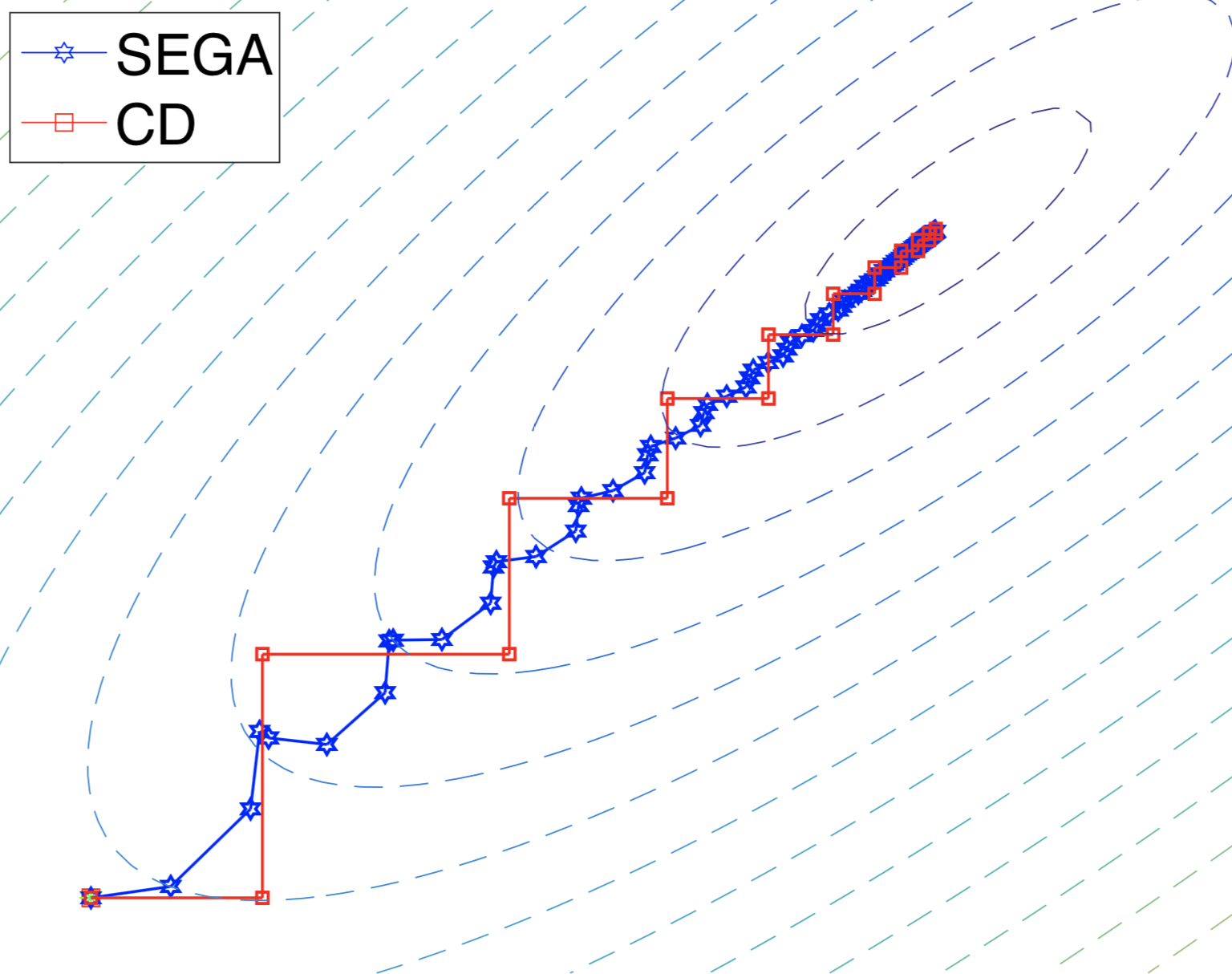
Figure 1: Iterates of SEGA and CD

2.1 SEGA as a variance-reduced method

As we shall show, both $h^{k}$ and $g^{k}$ are becoming better at approximating $\nabla f(x^{k})$ as the iterates $x^{k}$ approach the optimum. Hence, the variance of $g^{k}$ as an estimator of the gradient tends to zero, which means that SEGA is a variance-reduced algorithm. The structure of SEGA is inspired by the JackSketch algorithm introduced in [13]. However, as JackSketch is aimed at solving a finite-sum optimization problem with many components, it does not make much sense to apply it to (1). Indeed, when applied to (1) (with $R=0$, since JackSketch was analyzed for smooth optimization only), JackSketch reduces to gradient descent. While JackSketch performs Jacobian sketching (i.e., multiplying the Jacobian by a random matrix from the right, effectively sampling a subset of the gradients forming the finite sum), SEGA multiplies the Jacobian by a random matrix from the left. In doing so, SEGA becomes oblivious to the finite-sum structure and transforms into the gradient sketching mechanism described in (2).

2.2 SEGA versus coordinate descent

We now illustrate the above general setup on the simple example when ${\cal D}$ corresponds to a distribution over standard unit basis vectors in $\mathbb{R}^{n}$.

Example 2.1.

Let ${\bf B}={\rm Diag}(b_{1},\dots,b_{n})\succ 0$ and let ${\cal D}$ be defined as follows. We choose $\mathbf{S}_{k}=e_{i}$ with probability $p_{i}>0$, where $e_{1},e_{2},\dots,e_{n}$ are the unit basis vectors in $\mathbb{R}^{n}$. Then

$$h^{k+1}\overset{\eqref{eq:h^{k+1}}}{=}h^{k}+e_{i}^{\top}(\nabla f(x^{k})-h^{k})e_{i},$$ (8)

which can equivalently be written as $h^{k+1}_{i}=e_{i}^{\top}\nabla f(x^{k})$ and $h^{k+1}_{j}=h^{k}_{j}$ for $j\neq i$. Note that $h^{k+1}$ does not depend on ${\bf B}$. If we choose $\theta_{k}=\theta(\mathbf{S}_{k})=1/p_{i}$, then

$$\mathbb{E}_{{\cal D}}\left[\theta_{k}{\bf Z}_{k}\right]=\sum_{i=1}^{n}p_{i}\frac{1}{p_{i}}e_{i}(e_{i}^{\top}{\bf B}^{-1}e_{i})^{-1}e_{i}^{\top}=\sum_{i=1}^{n}\frac{e_{i}e_{i}^{\top}}{1/b_{i}}={\bf B}$$

which means that $\theta_{k}$ is a bias-correcting random variable. We then get

$$g^{k}\overset{\eqref{eq:g^k}}{=}h^{k}+\frac{1}{p_{i}}e_{i}^{\top}(\nabla f(x^{k})-h^{k})e_{i}.$$ (9)

In the setup of Example 2.1, both SEGA and CD obtain new gradient information in the form of a random partial derivative of $f$. However, the two methods process this information differently, and perform a different update:

• While SEGA allows for arbitrary proximal term, CD allows for separable proximal term only [48, 27, 12].

• While SEGA updates all coordinates in every iteration, CD updates a single coordinate only.

• If we force $h^{k}=0$ in SEGA and use coordinate sketches, the method transforms into CD.

Based on the above observations, we conclude that SEGA can be applied in more general settings for the price of potentially more expensive iterations. For intuition-building illustration of how SEGA works, Figure 1 shows the evolution of iterates of both SEGA and CD applied to minimizing a simple quadratic function in 2 dimensions. For more figures of this type, including the composite case where CD does not work, see Appendix F.1.

In Section 4 we show that SEGA enjoys the same theoretical iteration complexity rates as CD, up to a small constant factor. This remains true when comparing state-of-the-art variants of CD utilizing importance-sampling, parallelism/mini-batching and acceleration with the appropriate corresponding variants of SEGA.

Remark 2.2.

Nontrivial sketches $\mathbf{S}$ and metric ${\bf B}$ might, in some applications, bring a substantial speedup against the baseline choices mentioned in Example 2.1. Appendix C provides one setting where this can happen: there are problems where the gradient of $f$ always lies in a particular $d$-dimensional subspace of $\mathbb{R}^{n}$. In such a case, suitable choice of $\mathbf{S}$ and ${\bf B}$ leads to ${\cal O}\left(\tfrac{n}{d}\right)$–times faster convergence compared to the setup of Example 2.1. In Section 5.3 we numerically demonstrate this claim.

3 Convergence of SEGA for General Sketches

In this section we state a linear convergence result for SEGA (Algorithm 1) for general sketch distributions ${\cal D}$ under smoothness and strong convexity assumptions.

3.1 Smoothness assumptions

We will use the following general version of smoothness.

Assumption 3.1 (${\bf Q}$-smoothness).

Function $f$ is ${\bf Q}$-smooth with respect to ${\bf B}$, where ${\bf Q}\succ 0$ and ${\bf B}\succ 0$. That is, for all $x,y$, the following inequality is satisfied:

$$f(x)-f(y)-\langle\nabla f(y),x-y\rangle_{{\bf B}}\geq\frac{1}{2}\|\nabla f(x)-\nabla f(y)\|_{{\bf Q}}^{2},$$ (10)

Assumption 3.1 is not standard in the literature. However, as Lemma A.1 states, for ${\bf B}={\bf I}$ and ${\bf Q}={\bf M}^{-1}$, Assumption 3.1 is equivalent to ${\bf M}$-smoothness (see Assumption 3.2), which is a common assumption in modern analysis of CD methods. Hence, our assumption is more general than the commonly used assumption.

Assumption 3.2 (${\bf M}$-smoothness).

Function $f$ is ${\bf M}$-smooth for some matrix ${\bf M}\succ 0$. That is, for all $x,y$, the following inequality is satisfied:

$$f(x)\leq f(y)+\langle\nabla f(y),x-y\rangle+\frac{1}{2}\|x-y\|^{2}_{{\bf M}}.$$ (11)

Assumption 3.2 is fairly standard in the CD literature. It appears naturally in various application such as empirical risk minimization with linear predictors and is a baseline in the development of minibatch CD methods [43, 40, 38, 41]. We will adopt this notion in Section 4, when comparing SEGA to coordinate descent. Until then, let us consider the more general Assumption 3.1.

3.2 Main result

We are now ready to present one of the key theorems of the paper, which states that the iterates of SEGA converge linearly to the optimal solution.

Theorem 3.3.

Assume that $f$ is ${\bf Q}$–smooth with respect to ${\bf B}$, and $\mu$–strongly convex. Choose stepsize $\alpha>0$ and Lyapunov parameter $\sigma>0$ so that

$$\alpha\left(2({\bf C}-{\bf B})+\sigma\mu{\bf B}\right)\leq\sigma\mathbb{E}_{{\cal D}}\left[{\bf Z}\right],\qquad\alpha{\bf C}\leq\frac{1}{2}\left({\bf Q}-\sigma\mathbb{E}_{{\cal D}}\left[{\bf Z}\right]\right),$$ (12)

where ${\bf C}\overset{\text{def}}{=}\mathbb{E}_{{\cal D}}\left[\theta_{k}^{2}{\bf Z}_{k}\right]$. Fix $x^{0},h^{0}\in{\rm dom}(F)$ and let $x^{k},h^{k}$ be the random iterates produced by SEGA. Then

$$\mathbb{E}\left[{\Phi}^{k}\right]\leq(1-\alpha\mu)^{k}{\Phi}^{0},$$

where ${\Phi}^{k}\overset{\text{def}}{=}\|x^{k}-x^{*}\|^{2}_{{\bf B}}+\sigma\alpha\|h^{k}-\nabla f(x^{*})\|^{2}_{{\bf B}}$ is a Lyapunov function and $x^{*}$ is the solution of (1).

Note that the convergence of the Lyapunov function ${\Phi}^{k}$ implies both $x^{k}\rightarrow x^{*}$ and $h^{k}\rightarrow\nabla f(x^{*})$. The latter means that SEGA is variance reduced, in contrast to CD in the proximal setup with non-separable $R$, which does not converge to the solution.

To clarify on the assumptions, let us mention that if $\sigma$ is small enough so that ${\bf Q}-\sigma\mathbb{E}_{{\cal D}}\left[{\bf Z}\right]\succ 0$, one can always choose stepsize $\alpha$ satisfying

$$\alpha\leq\min\left\{\frac{\lambda_{\text{min}}(\mathbb{E}_{{\cal D}}\left[{\bf Z}\right])}{\lambda_{\max}(2\sigma^{-1}({\bf C}-{\bf B})+\mu{\bf B})},\frac{\lambda_{\min}({\bf Q}-\sigma\mathbb{E}_{{\cal D}}\left[{\bf Z}\right])}{2\lambda_{\max}({\bf C})}\right\}$$ (13)

and inequalities (12) will hold. Therefore, we get the next corollary.

Corollary 3.4.

If $\sigma<\frac{\lambda_{\min}({\bf Q})}{\lambda_{\max}(\mathbb{E}_{{\cal D}}\left[{\bf Z}\right])}$, $\alpha$ satisfies (13) and $k\geq\frac{1}{\alpha\mu}\log\frac{{\Phi}^{0}}{\epsilon}$, then $\mathbb{E}\left[\|x^{k}-x^{*}\|^{2}_{{\bf B}}\right]\leq\epsilon$.

As Theorem 3.3 is rather general, we also provide a simplified version thereof, complete with a simplified analysis (Theorem D.1 in Appendix D). In the simplified version we remove the proximal setting (i.e., we set $R=0$), assume $L$–smoothness, and only consider coordinate sketches with uniform probabilities. The result is provided as Corollary 3.5.

Corollary 3.5.

Let ${\bf B}={\bf I}$ and choose ${\cal D}$ to be the uniform distribution over unit basis vectors in $\mathbb{R}^{n}$. If the stepsize satisfies

$$0<\alpha\leq\min\left\{\frac{1-\frac{L\sigma}{n}}{2Ln},\frac{1}{n\left(\mu+\tfrac{2(n-1)}{\sigma}\right)}\right\},$$

then $\mathbb{E}_{{\cal D}}\left[{\Phi}^{k+1}\right]\leq(1-\alpha\mu){\Phi}^{k}$, therefore the iteration complexity is $\tilde{{\cal O}}(nL/\mu)$.

Remark 3.6.

In the fully general setting, one might choose $\alpha$ to be bigger than bound (13), which depends on eigen properties of matrices $\mathbb{E}_{{\cal D}}\left[{\bf Z}\right],{\bf C},{\bf Q},{\bf B}$, leading to a better overall complexity according to Corollary 3.4. However, in the simple case with ${\bf B}={\bf I}$, ${\bf Q}={\bf I}$ and $\mathbf{S}_{k}=e_{i_{k}}$ with uniform probabilities, bound (13) is tight.

4 Convergence of SEGA for Coordinate Sketches

In this section we compare SEGA with coordinate descent. We demonstrate that, specialized to a particular choice of the distribution ${\cal D}$ (where $\mathbf{S}$ is a random column submatrix of the identity matrix), which makes SEGA use the same random gradient information as that used in modern state-of-the-art randomized CD methods, SEGA attains, up to a small constant factor, the same convergence rate as CD methods.

Firstly, in Section 4.2 we develop SEGA with arbitrary “coordinate sketches” (Theorem 4.2). Then, in Section 4.3 we develop an accelerated variant of SEGA in a very general setup known as arbitrary sampling (see Theorem B.5) [43, 42, 39, 40, 6]. Lastly, Corollary 4.3 and Corollary 4.5 provide us with importance sampling for both nonaccelerated and accelerated method, which matches up to a constant factor cutting-edge coordinate descent rates [43, 3] under the same oracle and assumptions. Table 1 summarizes the results of this section. We provide a dedicated analysis for the methods from this section in Appendix B.

	CD	SEGA
Nonaccelerated method importance sampling, $b=1$	$\frac{{\rm Trace}({\bf M})}{\mu}\log\frac{1}{\epsilon}$ [36]	$8.55\cdot\frac{{\rm Trace}({\bf M})}{\mu}\log\frac{1}{\epsilon}$
Nonaccelerated method arbitrary sampling	$\left(\max_{i}\frac{v_{i}}{p_{i}\mu}\right)\log\frac{1}{\epsilon}$ [43]	$8.55\cdot\left(\max_{i}\frac{v_{i}}{p_{i}\mu}\right)\log\frac{1}{\epsilon}$
Accelerated method importance sampling, $b=1$	$1.62\cdot\frac{\sum_{i}\sqrt{{\bf M}_{ii}}}{\sqrt{\mu}}\log\frac{1}{\epsilon}$ [3]	$9.8\cdot\frac{\sum_{i}\sqrt{{\bf M}_{ii}}}{\sqrt{\mu}}\log\frac{1}{\epsilon}$
Accelerated method arbitrary sampling	$1.62\cdot\sqrt{\max_{i}\frac{v_{i}}{p_{i}^{2}\mu}}\log\frac{1}{\epsilon}$ [20]	$9.8\cdot\sqrt{\max_{i}\frac{v_{i}}{p_{i}^{2}\mu}}\log\frac{1}{\epsilon}$

Table 1: Complexity results for coordinate descent (CD) and our sketched gradient method (SEGA), specialized to coordinate sketching, for ${\bf M}$–smooth and $\mu$–strongly convex functions.

We now describe the setup and technical assumptions for this section. In order to facilitate a direct comparison with CD (which does not work with non-separable regularizer $R$), for simplicity we consider problem (1) in the simplified setting with $R\equiv 0$. Further, function $f$ is assumed to be ${\bf M}$–smooth (Assumption 3.2) and $\mu$–strongly convex.

4.1 Defining ${\cal D}$: samplings

In order to draw a direct comparison with general variants of CD methods (i.e., with those analyzed in the arbitrary sampling paradigm), we consider sketches in (3) that are column submatrices of the identity matrix: $\mathbf{S}={\bf I}_{S},$ where $S$ is a random subset (aka sampling) of $[n]\overset{\text{def}}{=}\{1,2,\dots,n\}$. Note that the columns of ${\bf I}_{S}$ are the standard basis vectors $e_{i}$ for $i\in S$ and hence

$$\mbox{Range}\left(\mathbf{S}\right)=\mbox{Range}\left(e_{i}\;:\;i\in S\right).$$

So, distribution ${\cal D}$ from which we draw matrices is uniquely determined by the distribution of sampling $S$. Given a sampling $S$, define $p=(p_{1},\dots,p_{n})\in\mathbb{R}^{n}$ to be the vector satisfying $p_{i}=\mathbb{P}\left(e_{i}\in\mbox{Range}\left(\mathbf{S}\right)\right)=\mathbb{P}\left(i\in S\right)$, and ${{\bf P}}$ to be the matrix for which

$${{\bf P}}_{ij}=\mathbb{P}\left(\{i,j\}\subseteq S\right).$$

Note that $p$ and ${{\bf P}}$ are the probability vector and probability matrix of sampling $S$, respectively [40]. We assume throughout the paper that $S$ is proper, i.e., we assume that $p_{i}>0$ for all $i$. State-of-the-art minibatch CD methods (including the ones we compare against [43, 20]) utilize large stepsizes related to the so-called ESO Expected Separable Overapproximation (ESO) [40] parameters $v=(v_{1},\dots,v_{n})$. ESO parameters play a key role in SEGA as well, and are defined next.

Assumption 4.1 (ESO).

There exists a vector $v$ satisfying the following inequality

$${{\bf P}}\circ{\bf M}\preceq{\rm Diag}(p){\rm Diag}(v),$$ (14)

where $\circ$ denotes the Hadamard (i.e., element-wise) product of matrices.

In case of single coordinate sketches, parameters $v$ are equal to coordinate-wise smoothness constants of $f$. An extensive study on how to choose them in general was performed in [40]. For notational brevity, let us set ${\bf\hat{P}}\overset{\text{def}}{=}{\rm Diag}(p)$ and ${\bf\hat{V}}\overset{\text{def}}{=}{\rm Diag}(v)$ throughout this section.

4.2 Non-accelerated method

We now state the convergence rate of (non-accelerated) SEGA for coordinate sketches with arbitrary sampling of subsets of coordinates. The corresponding CD method was developed in [43].

Theorem 4.2.

Assume that $f$ is ${\bf M}$–smooth and $\mu$–strongly convex. Denote ${\Psi}^{k}\overset{\text{def}}{=}f(x^{k})-f(x^{*})+\sigma\|h^{k}\|^{2}_{{\bf\hat{P}}^{-1}}$. Choose $\alpha,\sigma>0$ such that

$$\sigma{\bf I}-\alpha^{2}({\bf\hat{V}}{\bf\hat{P}}^{-1}-{\bf M})\succeq\gamma\mu\sigma{\bf\hat{P}}^{-1},$$ (15)

where $\gamma\overset{\text{def}}{=}\alpha-\alpha^{2}\max_{i}\{\tfrac{v_{i}}{p_{i}}\}-\sigma$. Then the iterates of SEGA satisfy $\mathbb{E}\left[{\Psi}^{k}\right]\leq(1-\gamma\mu)^{k}{\Psi}^{0}.$

We now give an importance sampling result for a coordinate version of SEGA. We recover, up to a constant factor, the same convergence rate as standard CD [36]. The probabilities we chose are optimal in our analysis and are proportional to the diagonal elements of matrix ${\bf M}$.

Corollary 4.3.

Assume that $f$ is ${\bf M}$–smooth and $\mu$–strongly convex. Suppose that ${\cal D}$ is such that at each iteration standard unit basis vector $e_{i}$ is sampled with probability $p_{i}\propto{\bf M}_{ii}$. If we choose $\alpha=\frac{0.232}{{\rm Trace}({\bf M})},\sigma=\frac{0.061}{{\rm Trace}({\bf M})}$, then $\mathbb{E}\left[{\Psi}^{k}\right]\leq\left(1-\frac{0.117\mu}{{\rm Trace}({\bf M})}\right)^{k}{\Psi}^{0}.$

The iteration complexities provided in Theorem 4.2 and Corollary 4.3 are summarized in Table 1. We also state that $\sigma,\alpha$ can be chosen so that (15) holds, and the rate from Theorem 4.2 coincides with the rate from Table 1.

Remark 4.4.

Theorem 4.2 and Corollary 4.3 hold even under a non-convex relaxation of strong convexity – Polyak-Łojasiewicz inequality: $\mu(f(x)-f(x^{*}))\leq\tfrac{1}{2}\|\nabla f(x)\|_{2}^{2}$. Therefore, SEGA also converges for a certain class of non-convex problems. For an overview on different relaxations of strong convexity, see [23].

4.3 Accelerated method

In this section, we propose an accelerated (in the sense of Nesterov’s method [33, 34]) version of SEGA, which we call ASEGA. The analogous accelerated CD method, in which a single coordinate is sampled in every iteration, was developed and analyzed in [3]. The general variant utilizing arbitrary sampling was developed and analyzed in [20].

1 Initialize : $x^{0}=y^{0}=z^{0}\in\mathbb{R}^{n}$; $h^{0}\in\mathbb{R}^{n}$; $S$; parameters $\alpha,\beta,\tau,\mu>0$

2 for $k=1,2,\dots$ do

      3 $x^{k}=(1-\tau)y^{k-1}+\tau z^{k-1}$

      4 Sample $\mathbf{S}_{k}={\bf I}_{S_{k}}$, where $S_{k}\sim S$, and compute $g^{k},h^{k+1}$ according to (4), (6)

      5 $y^{k}=x^{k}-\alpha{\bf\hat{P}}^{-1}g^{k}$

      6 $z^{k}=\frac{1}{1+\beta\mu}(z^{k}+\beta\mu x^{k}-\beta g^{k})$

      

Algorithm 2 ASEGA: Accelerated SEGA

The method and analysis is inspired by [2]. Due to space limitations and technicality of the content, we state the main theorem of this section in Appendix B.4. Here, we provide Corollary 4.5, which shows that Algorithm 2 with single coordinate sampling enjoys, up to a constant factor, the same convergence rate as state-of-the-art accelerated coordinate descent method NUACDM of Allen-Zhu et al. [3].

Corollary 4.5.

Let the sampling be defined as follows: $S=\{i\}$ with probability $p_{i}\propto\sqrt{{\bf M}_{ii}}$, for $i\in[n]$. Then there exist acceleration parameters and a Lyapunov function ${\Upsilon}^{k}$ such that $f(y^{k})-f(x^{*})\leq{\Upsilon}^{k}$ and

$$\mathbb{E}\left[{\Upsilon}^{k}\right]\leq(1-\tau)^{k}{\Upsilon}^{0}=\left(1-{\cal O}\left(\frac{\sqrt{\mu}}{\sum_{i}\sqrt{{\bf M}_{ii}}}\right)\right)^{k}{\Upsilon}^{0}.$$

The iteration complexity guarantees provided by Theorem B.5 and Corollary 4.5 are summarized in Table 1.

5 Experiments

In this section we perform numerical experiments to illustrate the potential of SEGA. Firstly, in Section 5.1, we compare it to projected gradient descent (PGD) algorithm. Then in Section 5.2, we study the performance of zeroth-order SEGA (when sketched gradients are being estimated through function value evaluations) and compare it to the analogous zeroth-order method. Lastly, in Section 5.3 we verify the claim from Remark 3.6 that in some applications, particular sketches and metric might lead to a significantly faster convergence. In the experiments where theory-supported stepsizes were used, we obtained them by precomputing strong convexity and smoothness measures.

5.1 Comparison to projected gradient

In this experiment, we illustrate the potential superiority of our method to PGD. We consider the $\ell_{2}$ ball constrained problem ($R$ is the indicator function of the unit ball) with the oracle providing the sketched gradient in the random Gaussian direction. As we mentioned in the introduction, a method moving in the gradient direction (analogue of CD), will not converge due to the proximal nature of the problem. Therefore, we can only compare against the projected gradient. However, in order to obtain the full gradient, one needs to gather $n$ sketched gradients and solve a linear system to recover the gradient. To illustrate this, we choose 4 different quadratic problems, according to Table 2 in the appendix. We stress that these are synthetic problems generated for the purpose of illustrating the potential of our method against a natural baseline. Figure 2 compares SEGA and PGD under various relative cost scenarios of solving the linear system compared to the cost of the oracle calls. The results show that SEGA significantly outperforms PGD as soon as solving the linear system is expensive, and is as fast as PGD even if solving the linear system comes for free.

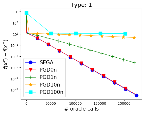
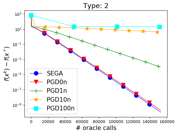
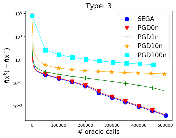
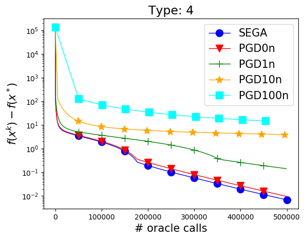
Figure 2: Convergence of SEGA and PGD on synthetic problems with $n=500$. The indicator “Xn” in the label indicates the setting where the cost of solving linear system is $Xn$ times higher comparing to the oracle call. Recall that a linear system is solved after each $n$ oracle calls. Stepsizes $1/\lambda_{\max}({\bf M})$ and $1/(n\lambda_{\max}({\bf M}))$ were used for PGD and SEGA, respectively.

5.2 Comparison to zeroth-order optimization methods

In this section, we compare SEGA to the random direct search (RDS) method [5] under a zeroth-order oracle for unconstrained optimization. For SEGA, we estimate the sketched gradient using finite differences. Note that RDS is a randomized version of the classical direct search method [21, 24, 25]. At iteration $k$, RDS moves to $\operatorname*{argmin}\left(f(x^{k}+\alpha^{k}s^{k}),f(x^{k}-\alpha^{k}s^{k}),f(x^{k})\right)$ for a random direction $s^{k}\sim{\cal D}$ and a suitable stepszie $\alpha^{k}$. For illustration, we choose $f$ to be a quadratic problem based on Table 2 and compare both Gaussian and coordinate directions. Figure 3 shows that SEGA outperforms RDS.

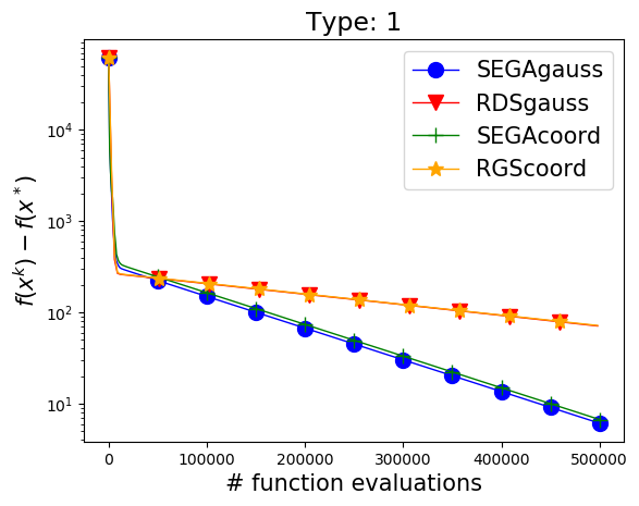
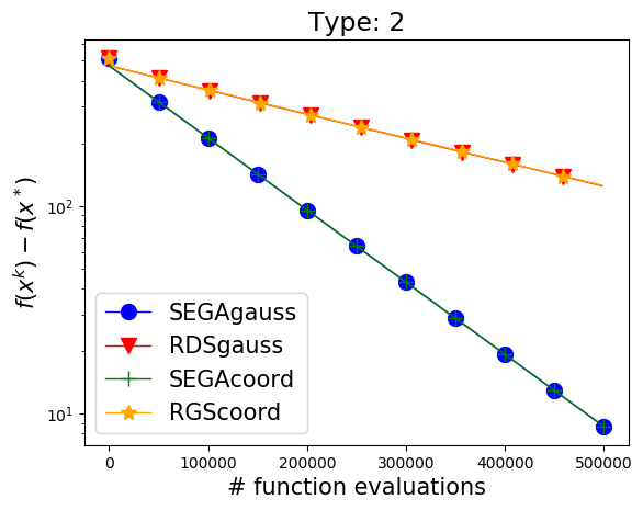
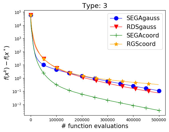
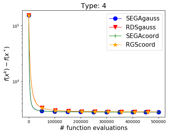
Figure 3: Comparison of SEGA and randomized direct search for various problems. Theory supported stepsizes were chosen for both methods. 500 dimensional problem.

5.3 Subspace SEGA: a more aggressive approach

As mentioned in Remark 3.6, well designed sketches are capable of exploiting structure of $f$ and lead to a better rate. We address this in detail Appendix C where we develop and analyze a subspace variant of SEGA.

To illustrate this phenomenon in a simple setting, we perform experiments for problem (1) with $f(x)=\|{\bf A}x-b\|^{2},$ where $b\in\mathbb{R}^{d}$ and ${\bf A}\in\mathbb{R}^{d\times n}$ has orthogonal rows, and with $R$ being the indicator function of the unit ball in $\mathbb{R}^{n}$. That is, we solve the problem

$$\min_{\|x\|_{2}\leq 1}\|{\bf A}x-b\|^{2}.$$

We assume that $n\gg d$. We compare two methods: naiveSEGA, which uses coordinate sketches, and subspaceSEGA, where sketches are chosen as rows of ${\bf A}$. Figure 4 indicates that subspaceSEGA outperforms naiveSEGA roughly by the factor $\tfrac{n}{d}$, as claimed in Appendix C.

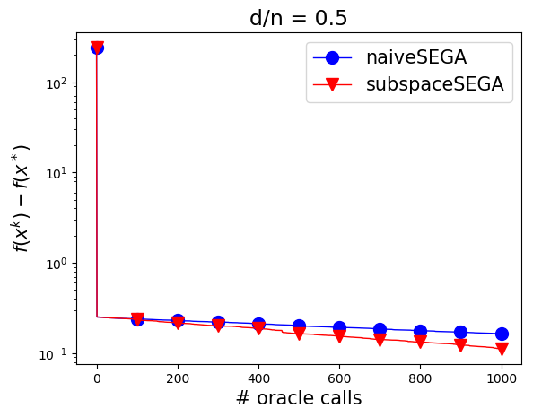
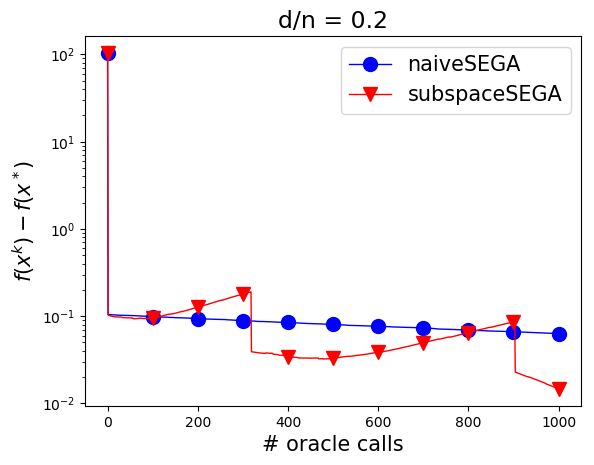
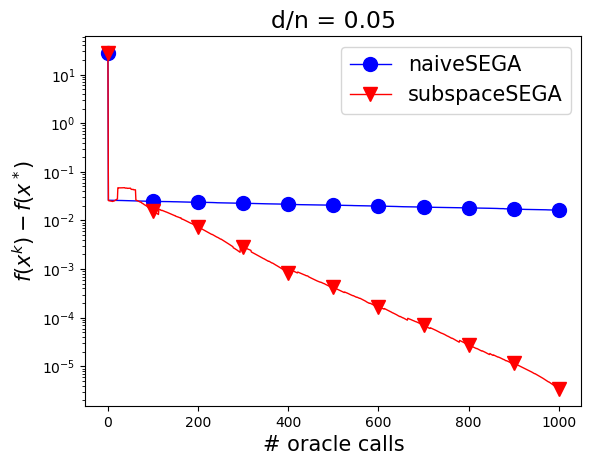
Figure 4: Comparison of SEGA with sketches from a correct subspace versus coordinate sketches naiveSEGA. Stepsize chosen according to theory. 1000 dimensional problem.

6 Conclusions and Extensions

6.1 Conclusions

We proposed SEGA, a method for solving composite optimization problems under a novel stochastic linear first order oracle. SEGA is variance-reduced, and this is achieved via sketch-and-project updates of gradient estimates. We provided an analysis for smooth and strongly convex functions and general sketches, and a refined analysis for coordinate sketches. For coordinate sketches we also proposed an accelerated variant of SEGA, and our theory matches that of state-of-the-art CD methods. However, in contrast to CD, SEGA can be used for optimization problems with a non-separable proximal term. We develop a more aggressive subspace variant of the method—subspaceSEGA—which leads to improvements in the $n\gg d$ regime. In the Appendix we give several further results, including simplified and alternative analyses of SEGA in the coordinate setup from Example 2.1. Our experiments are encouraging and substantiate our theoretical predictions.

6.2 Extensions

We now point to several potential extensions of our work.

Speeding up the general method.

We believe that it should be possible to extend ASEGA to the general setup from Theorem 3.3. In such a case, it might be possible to design metric ${\bf B}$ and distribution of sketches ${\cal D}$ so as to outperform accelerated proximal gradient methods [35, 4].

Biased gradient estimator.

Recall that SEGA uses unbiased gradient estimator $g^{k}$ for updating the iterates $x^{k}$ in a similar way JacSketch [13] or SAGA [10] do this for the stochastic finite sum optimization. Recently, a stochastic method for finite sum optimization using biased gradient estimators was proven to be more efficient [37]. Therefore, it might be possible to establish better properties for a biased variant of SEGA. To demonstrate the potential of this approach, in Appendix F.1 we plot the evolution of iterates for the very simple biased method which uses $h^{k}$ as an update for line 2 in Algorithm 1.

Applications.

We believe that SEGA might work well in applications where a zeroth-order approach is inevitable, such as reinforcement learning. We therefore believe that SEGA might be an efficient proximal method in some reinforcement learning applications. We also believe that communication-efficient variants of SEGA can be used for distributed training of machine learning models. This is because SEGA can be adapted to communicate sparse model updates only.

Appendix

Appendix A Proofs for Section 3

Lemma A.1.

Suppose that ${\bf B}={\bf I}$ and $f$ is twice differentiable. Assumption 3.1 is equivalent to Assumption 3.2 for ${\bf Q}={\bf M}^{-1}$.

Proof: We first establish that Assumption 3.1 implies Assumption 3.2. Summing up (10) for $(x,y)$ and $(y,x)$ yields

$$\langle\nabla f(x)-\nabla f(y),x-y\rangle\geq\|\nabla f(x)-\nabla f(y)\|_{{\bf Q}}^{2}.$$

Using Cauchy Schwartz inequality we obtain

$$\|x-y\|_{{\bf Q}^{-1}}\geq\|\nabla f(x)-\nabla f(y)\|_{{\bf Q}}.$$

By the mean value theorem, there is $z\in[x,y]$ such that $\nabla f(x)-\nabla f(y)=\nabla^{2}f(z)(x-y)$. Thus

$$\|x-y\|_{{\bf Q}^{-1}}\geq\|x-y\|_{\nabla^{2}f(z){\bf Q}\nabla^{2}f(z)}.$$

The above is equivalent to

$$\left(\nabla^{2}f(z)\right)^{-\frac{1}{2}}{\bf Q}^{-1}\left(\nabla^{2}f(z)\right)^{-\frac{1}{2}}\succeq\left(\nabla^{2}f(z)\right)^{\frac{1}{2}}{\bf Q}\left(\nabla^{2}f(z)\right)^{\frac{1}{2}}$$

Note that for any ${\bf M}^{\prime}\succ 0$ we have ${\bf M}^{\prime}\succeq{\bf M}^{-1}$ if and only if ${\bf M}\succeq{\bf I}$. Thus

$$\left(\nabla^{2}f(z)\right)^{-\frac{1}{2}}{\bf Q}^{-1}\left(\nabla^{2}f(z)\right)^{-\frac{1}{2}}\succeq{\bf I},$$

which is equivalent to ${\bf Q}^{-1}\succeq\nabla^{2}f(z)$. To establish the other direction, denote $\phi(y)=f(y)-\langle\nabla f(x),y\rangle$. Clearly, $x$ is minimizer of $\phi$ and therefore we have

$$\phi(x)\leq\phi(x-{\bf M}^{-1}\nabla f(y))\leq\phi(y)-\frac{1}{2}\|\nabla f(y)\|^{2}_{{\bf M}^{-1}},$$

which is exactly (10) for ${\bf Q}={\bf M}^{-1}$. ∎

Lemma A.2.

For ${\bf B}\succ 0$ and ${\bf Z}_{k}\overset{\text{def}}{=}\mathbf{S}_{k}(\mathbf{S}_{k}^{\top}{\bf B}^{-1}\mathbf{S}_{k})^{\dagger}\mathbf{S}_{k}^{\top}$, then

$${\bf Z}_{k}^{\top}{\bf B}^{-1}{\bf Z}_{k}={\bf Z}_{k}.$$ (16)

Proof: It is a property of pseudo-inverse that for any matrices ${\bf A},{\bf B}$ it holds $(({\bf A}{\bf B})^{\dagger})^{\top}=({\bf B}^{\top}{\bf A}^{\top})^{\dagger}$, so ${\bf Z}_{k}^{\top}={\bf Z}_{k}$. Moreover, we also know for any ${\bf A}$ that ${\bf A}^{\dagger}{\bf A}{\bf A}^{\dagger}={\bf A}^{\dagger}$ and, thus,

$${\bf Z}_{k}^{\top}{\bf B}^{-1}{\bf Z}_{k}=\mathbf{S}_{k}(\mathbf{S}_{k}^{\top}{\bf B}^{-1}\mathbf{S}_{k})^{\dagger}\mathbf{S}_{k}^{\top}{\bf B}^{-1}\mathbf{S}_{k}(\mathbf{S}_{k}^{\top}{\bf B}^{-1}\mathbf{S}_{k})^{\dagger}\mathbf{S}_{k}^{\top}=\mathbf{S}_{k}(\mathbf{S}_{k}^{\top}{\bf B}^{-1}\mathbf{S}_{k})^{\dagger}\mathbf{S}_{k}^{\top}={\bf Z}_{k}.$$

∎

A.1 Proof of Theorem 3.3

We first state two lemmas which will be crucial for the analysis. They characterize key properties of the gradient learning process (4), (6) and will be used later to bound expected distances of both $h^{k+1}$ and $g^{k}$ from $\nabla f(x^{*})$. The proofs are provided in Appendix A.2 and A.3 respectively

Lemma A.3.

For all $v\in\mathbb{R}^{n}$ we have

$$\mathbb{E}_{{\cal D}}\left[\|h^{k+1}-v\|_{{\bf B}}^{2}\right]=\|h^{k}-v\|_{{\bf B}-\mathbb{E}_{{\cal D}}\left[{\bf Z}\right]}^{2}+\|\nabla f(x^{k})-v\|_{\mathbb{E}_{{\cal D}}\left[{\bf Z}\right]}^{2}.$$ (17)

Lemma A.4.

Let ${\bf C}\overset{\text{def}}{=}\mathbb{E}_{{\cal D}}\left[\theta^{2}{\bf Z}\right]$. Then for all $v\in\mathbb{R}^{n}$ we have

$$\mathbb{E}_{{\cal D}}\left[\|g^{k}-v\|_{\bf B}^{2}\right]\leq 2\|\nabla f(x^{k})-v\|^{2}_{\bf C}+2\|h^{k}-v\|^{2}_{{\bf C}-{\bf B}}.$$

For notational simplicity, it will be convenient to define Bregman divergence between $x$ and $y$:

$$D_{f}(x,y)\overset{\text{def}}{=}f(x)-f(y)-\langle\nabla f(y)),x-y\rangle_{{\bf B}}$$

We can now proceed with the proof of Theorem 3.3. Let us start with bounding the first term in the expression for ${\Phi}^{k+1}$. From Lemma A.4 and strong convexity it follows that

$$\mathbb{E}_{{\cal D}}\left[\|x^{k+1}-x^{*}\|^{2}_{\bf B}\right] = \mathbb{E}_{{\cal D}}\left[\|\mathop{\mathrm{prox}}\nolimits_{\alpha R}(x^{k}-\alpha g^{k})-\mathop{\mathrm{prox}}\nolimits_{\alpha R}(x^{*}-\alpha\nabla f(x^{*}))\|^{2}_{\bf B}\right]$$

$$\leq \mathbb{E}_{{\cal D}}\left[\|x^{k}-\alpha g^{k}-(x^{*}-\alpha\nabla f(x^{*}))\|^{2}_{\bf B}\right]$$

$$= \|x^{k}-x^{*}\|^{2}_{\bf B}-2\alpha\mathbb{E}_{{\cal D}}\left[(g^{k}-\nabla f(x^{*}))^{\top}{\bf B}(x^{k}-x^{*})\right]$$

$$\qquad+\alpha^{2}\mathbb{E}_{{\cal D}}\left[\|g^{k}-\nabla f(x^{*})\|^{2}_{\bf B}\right]$$

$$\leq \|x^{k}-x^{*}\|^{2}_{\bf B}-2\alpha(\nabla f(x^{k})-\nabla f(x^{*}))^{\top}{\bf B}(x^{k}-x^{*})$$

$$\qquad+2\alpha^{2}\|\nabla f(x^{k})-\nabla f(x^{*})\|^{2}_{\bf C}+2\alpha^{2}\|h^{k}-\nabla f(x^{*})\|^{2}_{{\bf C}-{\bf B}}$$

$$\leq \|x^{k}-x^{*}\|^{2}_{\bf B}-\alpha\mu\|x^{k}-x^{*}\|^{2}_{\bf B}-2\alpha D_{f}(x^{k},x^{*})$$

$$\qquad+2\alpha^{2}\|\nabla f(x^{k})-\nabla f(x^{*})\|^{2}_{\bf C}+2\alpha^{2}\|h^{k}-\nabla f(x^{*})\|^{2}_{{\bf C}-{\bf B}}.$$

Using Assumption 3.1 we get

$$-2\alpha D_{f}(x^{k},x^{*})\leq-\alpha\|\nabla f(x^{k})-\nabla f(x^{*})\|^{2}_{\bf Q}.$$

As for the second term in ${\Phi}^{k+1}$, we have by Lemma A.3

$$\alpha\sigma\mathbb{E}_{{\cal D}}\left[\|h^{k+1}-\nabla f(x^{*})\|^{2}_{\bf B}\right]=\alpha\sigma\|h^{k}-\nabla f(x^{*})\|^{2}_{{\bf B}-\mathbb{E}_{{\cal D}}\left[{\bf Z}\right]}+\alpha\sigma\|\nabla f(x^{k})-\nabla f(x^{*})\|^{2}_{\mathbb{E}_{{\cal D}}\left[{\bf Z}\right]}$$

Combining it into Lyapunov function ${\Phi}^{k}$,

$${\Phi}^{k+1} \leq (1-\alpha\mu)\|x^{k}-x^{*}\|^{2}_{\bf B}+\alpha\sigma\|h^{k}-\nabla f(x^{*})\|^{2}_{{\bf B}-\mathbb{E}_{{\cal D}}\left[{\bf Z}\right]}+2\alpha^{2}\|h^{k}-\nabla f(x^{*})\|^{2}_{{\bf C}-{\bf B}}$$

$$+\alpha\sigma\|\nabla f(x^{k})-\nabla f(x^{*})\|^{2}_{\mathbb{E}_{{\cal D}}\left[{\bf Z}\right]}+2\alpha^{2}\|\nabla f(x^{k})-\nabla f(x^{*})\|^{2}_{\bf C}-\alpha\|\nabla f(x^{k})-\nabla f(x^{*})\|^{2}_{\bf Q}.$$

To see that this gives us the theorem’s statement, consider first

$$\alpha\sigma\mathbb{E}_{{\cal D}}\left[{\bf Z}\right]+2\alpha^{2}{\bf C}-\alpha{\bf Q}=2\alpha(\alpha{\bf C}-\tfrac{1}{2}({\bf Q}-\sigma\mathbb{E}_{{\cal D}}\left[{\bf Z}\right]))\leq 0,$$

so we can drop norms related to $\nabla f(x^{k})-\nabla f(x^{*})$. Next, we have

$$\alpha\sigma({\bf B}-\mathbb{E}_{{\cal D}}\left[{\bf Z}\right])+2\alpha^{2}({\bf C}-{\bf B}) = \alpha\left(\alpha(2({\bf C}-{\bf B})+\sigma\mu{\bf B})-\mathbb{E}_{{\cal D}}\left[{\bf Z}\right]\right)+\sigma\alpha(1-\alpha\mu){\bf B}$$

$$\leq \sigma\alpha(1-\alpha\mu){\bf B},$$

which follows from our assumption on $\alpha$. ∎

A.2 Proof of Lemma A.3

Proof: Keeping in mind that ${\bf Z}_{k}^{\top}={\bf Z}_{k}$ and $({\bf B}^{-1})^{\top}={\bf B}^{-1}$, we first write

$$\mathbb{E}_{{\cal D}}\left[\|h^{k+1}-v\|_{\bf B}^{2}\right] \overset{\eqref{eq:988fgf}}{=} \mathbb{E}_{{\cal D}}\left[\left\|h^{k}+{\bf B}^{-1}{\bf Z}_{k}(\nabla f(x^{k})-h^{k})-v\right\|_{\bf B}^{2}\right]$$

$$= \mathbb{E}_{{\cal D}}\left[\left\|\left({\bf I}-{\bf B}^{-1}{\bf Z}_{k}\right)(h^{k}-v)+{\bf B}^{-1}{\bf Z}_{k}(\nabla f(x^{k})-v)\right\|_{\bf B}^{2}\right]$$

$$= \mathbb{E}_{{\cal D}}\left[\left\|\left({\bf I}-{\bf B}^{-1}{\bf Z}_{k}\right)(h^{k}-v)\right\|_{\bf B}^{2}\right]+\mathbb{E}_{{\cal D}}\left[\left\|{\bf B}^{-1}{\bf Z}_{k}(\nabla f(x^{k})-v)\right\|_{\bf B}^{2}\right]$$

$$\qquad+2(h^{k}-v)^{\top}\mathbb{E}_{{\cal D}}\left[\left({\bf I}-{\bf B}^{-1}{\bf Z}_{k}\right)^{\top}{\bf B}{\bf B}^{-1}{\bf Z}_{k}\right](\nabla f(x^{k})-v)$$

$$= (h^{k}-v)^{\top}\mathbb{E}_{{\cal D}}\left[\left({\bf I}-{\bf B}^{-1}{\bf Z}_{k}\right)^{\top}{\bf B}\left({\bf I}-{\bf B}^{-1}{\bf Z}_{k}\right)\right](h^{k}-v)$$

$$\qquad+(\nabla f(x^{k})-v)^{\top}\mathbb{E}_{{\cal D}}\left[{\bf Z}_{k}{\bf B}^{-1}{\bf B}{\bf B}^{-1}{\bf Z}_{k}\right](\nabla f(x^{k})-v)$$

$$\qquad+2(h^{k}-v)^{\top}\mathbb{E}_{{\cal D}}\left[{\bf Z}_{k}-{\bf Z}_{k}{\bf B}^{-1}{\bf Z}_{k}\right](\nabla f(x^{k})-v).$$

By Lemma A.2 we have ${\bf Z}_{k}{\bf B}^{-1}{\bf Z}_{k}={\bf Z}_{k}$, so the last term in the expression above is equal to 0. As for the other two, expanding the matrix factor in the first term leads to

$$\mathbb{E}_{{\cal D}}\left[\left({\bf I}-{\bf B}^{-1}{\bf Z}_{k}\right)^{\top}{\bf B}\left({\bf I}-{\bf B}^{-1}{\bf Z}_{k}\right)\right] = \mathbb{E}_{{\cal D}}\left[\left({\bf I}-{\bf Z}_{k}{\bf B}^{-1}\right){\bf B}\left({\bf I}-{\bf B}^{-1}{\bf Z}_{k}\right)\right]$$

$$= \mathbb{E}_{{\cal D}}\left[{\bf B}-{\bf Z}_{k}{\bf B}^{-1}{\bf B}-{\bf B}{\bf B}^{-1}{\bf Z}_{k}+{\bf Z}_{k}{\bf B}^{-1}{\bf B}{\bf B}^{-1}{\bf Z}_{k}\right]$$

$$= {\bf B}-\mathbb{E}_{{\cal D}}\left[{\bf Z}_{k}\right].$$

We, thereby, have derived

$$\mathbb{E}_{{\cal D}}\left[\|h^{k+1}-v\|_{\bf B}^{2}\right] = (h^{k}-v)^{\top}\left({\bf B}-\mathbb{E}_{{\cal D}}\left[{\bf Z}_{k}\right]\right)(h^{k}-v)$$

$$\quad+(\nabla f(x^{k})-v)^{\top}\mathbb{E}_{{\cal D}}\left[{\bf Z}_{k}{\bf B}^{-1}{\bf Z}_{k}\right](\nabla f(x^{k})-v)$$

$$= \|h^{k}-v\|_{{\bf B}-\mathbb{E}_{{\cal D}}\left[{\bf Z}\right]}^{2}+\|\nabla f(x^{k})-v\|_{\mathbb{E}_{{\cal D}}\left[{\bf Z}\right]}^{2}.$$

∎

A.3 Proof of Lemma A.4

Proof: Throughout this proof, we will use without any mention that ${\bf Z}_{k}^{\top}={\bf Z}_{k}$.

Writing $g^{k}-v=a+b$, where $a\overset{\text{def}}{=}({\bf I}-\theta_{k}{\bf B}^{-1}{\bf Z}_{k})(h^{k}-v)$ and $b\overset{\text{def}}{=}\theta_{k}{\bf B}^{-1}{\bf Z}_{k}(\nabla f(x^{k})-v)$, we get $\|g^{k}\|_{\bf B}^{2}\leq 2(\|a\|_{\bf B}^{2}+\|b\|_{\bf B}^{2})$. Using Lemma A.2 and the definition of $\theta_{k}$ yields

$$\mathbb{E}_{{\cal D}}\left[\|a\|_{\bf B}^{2}\right] = \mathbb{E}_{{\cal D}}\left[\|\left({\bf I}-\theta_{k}{\bf B}^{-1}{\bf Z}_{k}\right)(h^{k}-v)\|_{\bf B}^{2}\right]$$

$$= (h^{k}-v)^{\top}\mathbb{E}_{{\cal D}}\left[\left({\bf I}-\theta_{k}{\bf Z}_{k}{\bf B}^{-1}\right){\bf B}\left({\bf I}-\theta_{k}{\bf B}^{-1}{\bf Z}_{k}\right)\right](h^{k}-v)$$

$$= (h^{k}-v)^{\top}\mathbb{E}_{{\cal D}}\left[\left({\bf B}-\theta_{k}{\bf Z}_{k}{\bf B}^{-1}{\bf B}-{\bf B}\theta_{k}{\bf B}^{-1}{\bf Z}_{k}+\theta_{k}^{2}{\bf Z}_{k}{\bf B}^{-1}{\bf B}{\bf B}^{-1}{\bf Z}_{k}\right)\right](h^{k}-v)$$

$$= (h^{k}-v)^{\top}\mathbb{E}_{{\cal D}}\left[\left({\bf B}-2{\bf B}+\theta_{k}^{2}{\bf Z}_{k}\right)\right](h^{k}-v)$$

$$= \|h^{k}-v\|^{2}_{\mathbb{E}_{{\cal D}}\left[\theta^{2}{\bf Z}\right]-{\bf B}}.$$

Similarly, the second term in the upper bound on $g^{k}$ can be rewritten as

$$\mathbb{E}_{{\cal D}}\left[\|b\|_{\bf B}^{2}\right] = \mathbb{E}_{{\cal D}}\left[\|\theta_{k}{\bf B}^{-1}{\bf Z}_{k}(\nabla f(x^{k})-v)\|^{2}_{\bf B}\right]$$

$$= (\nabla f(x^{k})-v)^{\top}\mathbb{E}_{{\cal D}}\left[\theta_{k}^{2}{\bf Z}_{k}{\bf B}^{-1}{\bf B}{\bf B}^{-1}{\bf Z}_{k}\right](\nabla f(x^{k})-v)$$

$$= \|\nabla f(x^{k})-v\|^{2}_{{\bf C}}.$$

Combining the pieces, we get the claim. ∎

Appendix B Proofs for Section 4

B.1 Technical Lemmas

We first start with an analogue of Lemma A.4 allowing for a norm different from $\|\cdot\|_{\bf B}$. We remark that matrix ${\bf Q}^{\prime}$ in the lemma is not to be confused with the smoothness matrix ${\bf Q}$ from Assumption 3.1.

Lemma B.1.

Let ${\bf Q}^{\prime}\succ 0$. The variance of $g^{k}$ as an estimator of $\nabla f(x^{k})$ can be bounded as follows:

$$\frac{1}{2}\mathbb{E}_{{\cal D}}\left[\|g^{k}\|_{{\bf Q}^{\prime}}^{2}\right]\leq\|h^{k}\|_{{\bf\hat{P}}^{-1}({{\bf P}}\circ{\bf Q}^{\prime}){\bf\hat{P}}^{-1}-{\bf Q}^{\prime}}^{2}+\|\nabla f(x^{k})\|^{2}_{{\bf\hat{P}}^{-1}({{\bf P}}\circ{\bf Q}^{\prime}){\bf\hat{P}}^{-1}}.$$ (18)

Proof: Denote $\mathbf{S}_{k}$ to be a matrix with columns $e_{i}$ for $i\in\mbox{Range}\left(\mathbf{S}_{k}\right)$. We first write

$$g^{k}=\underbrace{h^{k}-{\bf\hat{P}}^{-1}\mathbf{S}_{k}\mathbf{S}_{k}^{\top}h^{k}}_{a}+\underbrace{{\bf\hat{P}}^{-1}\mathbf{S}_{k}\mathbf{S}_{k}^{\top}\nabla f(x^{k})}_{b}.$$

Let us bound the expectation of each term individually. The first term is equal to

$$\mathbb{E}_{{\cal D}}\left[\|a\|_{{\bf Q}^{\prime}}^{2}\right] = \mathbb{E}_{{\cal D}}\left[\left\|\left({\bf I}-{\bf\hat{P}}^{-1}\mathbf{S}_{k}\mathbf{S}_{k}^{\top}\right)h^{k}\right\|_{{\bf Q}^{\prime}}^{2}\right]$$

$$= (h^{k})^{\top}\mathbb{E}_{{\cal D}}\left[\left({\bf I}-{\bf\hat{P}}^{-1}\mathbf{S}_{k}\mathbf{S}_{k}^{\top}\right)^{\top}{\bf Q}^{\prime}\left({\bf I}-{\bf\hat{P}}^{-1}\mathbf{S}_{k}\mathbf{S}_{k}^{\top}\right)\right]h^{k}$$

$$= (h^{k})^{\top}\mathbb{E}_{{\cal D}}\left[\left({\bf Q}^{\prime}-{\bf\hat{P}}^{-1}\mathbf{S}_{k}\mathbf{S}_{k}^{\top}{\bf Q}^{\prime}-{\bf Q}^{\prime}\mathbf{S}_{k}\mathbf{S}_{k}^{\top}{\bf\hat{P}}^{-1}\right)\right]h^{k}$$

$$\qquad\qquad+(h^{k})^{\top}\mathbb{E}_{{\cal D}}\left[\left({\bf\hat{P}}^{-1}\mathbf{S}_{k}\mathbf{S}_{k}^{\top}{\bf Q}^{\prime}\mathbf{S}_{k}\mathbf{S}_{k}^{\top}{\bf\hat{P}}^{-1}\right)\right]h^{k}$$

$$= (h^{k})^{\top}\left({\bf\hat{P}}^{-1}({{\bf P}}\circ{\bf Q}^{\prime}){\bf\hat{P}}^{-1}-{\bf Q}^{\prime}\right)h^{k}.$$

The second term can be bounded as

$$\mathbb{E}_{{\cal D}}\left[\|b\|_{{\bf Q}^{\prime}}^{2}\right] = \mathbb{E}_{{\cal D}}\left[\left\|{\bf\hat{P}}^{-1}\mathbf{S}_{k}^{\top}\nabla f(x^{k})\mathbf{S}_{k}\right\|_{{\bf Q}^{\prime}}^{2}\right]=\mathbb{E}_{{\cal D}}\left[\|\nabla f(x^{k})\|^{2}_{{\bf\hat{P}}^{-1}\mathbf{S}_{k}\mathbf{S}_{k}^{\top}{\bf Q}^{\prime}\mathbf{S}_{k}\mathbf{S}_{k}^{\top}{\bf\hat{P}}^{-1}}\right]$$

$$= \|\nabla f(x^{k})\|^{2}_{{\bf\hat{P}}^{-1}({{\bf P}}\circ{\bf Q}^{\prime}){\bf\hat{P}}^{-1}}$$

It remains to combine the two bounds. ∎

We also state the analogue of Lemma A.3, which allows for a different norm as well.

Lemma B.2.

For all diagonal ${\bf D}\succ 0$ we have

$$\mathbb{E}_{{\cal D}}\left[\|h^{k+1}\|_{{\bf D}}^{2}\right]=\|h^{k}\|_{{\bf D}-{\bf\hat{P}}{\bf D}}^{2}+\|\nabla f(x^{k})\|_{{\bf\hat{P}}{\bf D}}^{2}.$$ (19)

Proof: Denote $\mathbf{S}_{k}$ to be a matrix with columns $e_{i}$ for $i\in\mathbf{S}_{k}$. We first write

$$h^{k+1}=h^{k}-\mathbf{S}_{k}\mathbf{S}_{k}^{\top}h^{k}+\mathbf{S}_{k}\mathbf{S}_{k}^{\top}\nabla f(x^{k}).$$

Therefore

$$\mathbb{E}_{{\cal D}}\left[\|h^{k+1}\|_{{\bf D}}^{2}\right] = \mathbb{E}_{{\cal D}}\left[\left\|({\bf I}-\mathbf{S}_{k}\mathbf{S}_{k}^{\top})h^{k}+\mathbf{S}_{k}\mathbf{S}_{k}^{\top}\nabla f(x^{k})\right\|_{{\bf D}}^{2}\right]$$

$$= \mathbb{E}_{{\cal D}}\left[\left\|({\bf I}-\mathbf{S}_{k}\mathbf{S}_{k}^{\top})h^{k}\right\|_{{\bf D}}^{2}\right]+\mathbb{E}_{{\cal D}}\left[\left\|\mathbf{S}_{k}\mathbf{S}_{k}^{\top}\nabla f(x^{k})\right\|_{{\bf D}}^{2}\right]$$

$$\qquad+2\mathbb{E}_{{\cal D}}\left[{h^{k}}^{\top}({\bf I}-\mathbf{S}_{k}\mathbf{S}_{k}^{\top}){\bf D}\mathbf{S}_{k}\mathbf{S}_{k}^{\top}\nabla f(x^{k})\right]$$

$$= \|h^{k}\|_{{\bf D}-{\bf\hat{P}}{\bf D}}^{2}+\|\nabla f(x^{k})\|_{{\bf\hat{P}}{\bf D}}^{2}.$$

∎

B.2 Proof of Theorem 4.2

Proof: Throughout the proof, we will use the following Lyapunov function:

$${\Psi}^{k}\overset{\text{def}}{=}f(x^{k})-f(x^{*})+\sigma\|h^{k}\|^{2}_{{\bf P}^{-1}}.$$

Following similar steps to what we did before, we obtain

$$\mathbb{E}\left[{\Psi}^{k+1}\right] \stackrel{{\scriptstyle\eqref{eq:M_smooth}}}{{\leq}} f(x^{k})-f(x^{*})+\alpha\mathbb{E}\left[\langle\nabla f(x^{k}),g^{k}\rangle\right]+\frac{\alpha^{2}}{2}\mathbb{E}\left[\|g^{k}\|_{\bf M}^{2}\right]+\sigma\mathbb{E}\left[\|h^{k+1}\|^{2}_{{\bf\hat{P}}^{-1}}\right]$$

$$= f(x^{k})-f(x^{*})-\alpha\|\nabla f(x^{k})\|_{2}^{2}+\frac{\alpha^{2}}{2}\mathbb{E}\left[\|g^{k}\|_{\bf M}^{2}\right]+\sigma\mathbb{E}\left[\|h^{k+1}\|^{2}_{{\bf\hat{P}}^{-1}}\right]$$

$$\stackrel{{\scriptstyle\eqref{eq:almost_eso_g}}}{{\leq}} f(x^{k})-f(x^{*})-\alpha\|\nabla f(x^{k})\|_{2}^{2}+\alpha^{2}\|\nabla f(x^{k})\|^{2}_{{\bf\hat{P}}^{-1}({{\bf P}}\circ{\bf M}){\bf\hat{P}}^{-1}}+\alpha^{2}\|h^{k}\|^{2}_{{\bf\hat{P}}^{-1}({{\bf P}}\circ{\bf M}){\bf\hat{P}}^{-1}-{\bf M}}$$

$$\qquad+\sigma\mathbb{E}\left[\|h^{k+1}\|^{2}_{{\bf\hat{P}}^{-1}}\right].$$

This is the place where the ESO assumption comes into play. By applying it to the right-hand side of the bound above, we obtain

$$\mathbb{E}\left[{\Psi}^{k+1}\right] \stackrel{{\scriptstyle\eqref{eq:ESO}}}{{\leq}} f(x^{k})-f(x^{*})-\alpha\|\nabla f(x^{k})\|_{2}^{2}+\alpha^{2}\|\nabla f(x^{k})\|^{2}_{{\bf\hat{V}}{\bf\hat{P}}^{-1}}+\alpha^{2}\|h^{k}\|^{2}_{{\bf\hat{V}}{\bf\hat{P}}^{-1}-{\bf M}}$$

$$\qquad+\sigma\mathbb{E}\left[\|h^{k+1}\|^{2}_{{\bf\hat{P}}^{-1}}\right]$$

$$\stackrel{{\scriptstyle\eqref{eq:h_dec_general}}}{{=}} f(x^{k})-f(x^{*})-\alpha\|\nabla f(x^{k})\|_{2}^{2}+\alpha^{2}\|\nabla f(x^{k})\|^{2}_{{\bf\hat{V}}{\bf\hat{P}}^{-1}}+\alpha^{2}\|h^{k}\|^{2}_{{\bf\hat{V}}{\bf\hat{P}}^{-1}-{\bf M}}$$

$$\qquad+\sigma\|\nabla f(x^{k})\|_{2}^{2}+\sigma\|h^{k}\|^{2}_{{\bf\hat{P}}^{-1}-{\bf I}}$$

$$= f(x^{k})-f(x^{*})-\left(\alpha-\alpha^{2}\max_{i}\frac{v_{i}}{p_{i}}-\sigma\right)\|\nabla f(x^{k})\|_{2}^{2}$$

$$\qquad+\|h^{k}\|^{2}_{\alpha^{2}({\bf\hat{V}}{\bf\hat{P}}^{-1}-{\bf M})+\sigma({\bf\hat{P}}^{-1}-{\bf I})}.$$

Due to Polyak-Łojasiewicz inequality, we can further upper bound the last expression by

$$\left(1-\left(\alpha-\alpha^{2}\max_{i}\frac{v_{i}}{p_{i}}-\sigma\right)\mu\right)(f(x^{k})-f(x^{*}))+\|h^{k}\|^{2}_{\alpha^{2}({\bf\hat{V}}{\bf P}^{-1}-{\bf M})+\sigma({\bf P}^{-1}-{\bf I})}.$$

To finish the proof, it remains to use (15). ∎

B.3 Proof of Corollary 4.3

The claim was obtained by choosing carefully $\alpha$ and $\sigma$ using numerical grid search. Note that by strong convexity we have ${\bf I}\succeq\mu{\rm Diag}({\bf M})^{-1}$, so we can satisfy assumption (15). Then, the claim follows immediately noticing that we can also set ${\bf\hat{V}}={\rm Diag}({\bf M})$ while maintaining

$$\left(\alpha-\alpha^{2}\max_{i}\frac{{\bf M}_{ii}}{p_{i}}-\sigma\right)\geq\frac{0.117}{{\rm Trace}({\bf M})}.$$

B.4 Accelerated SEGA with arbitrary sampling

Before establishing the main theorem, we first state two technical lemmas which will be crucial for the analysis. First one, Lemma B.3 provides a key inequality following from (2). The second one, Lemma B.4, analyzes update (2) and was technically established throughout the proof of Theorem 4.2. We include a proof of lemmas in Appendix B.5 and B.6 respectively.

Lemma B.3.

For every $u\in\mathbb{R}^{n}$ we have

$$\beta\langle\nabla f(x^{k+1}),z^{k}-u\rangle-\frac{\beta\mu}{2}\|x^{k+1}-u\|_{2}^{2}$$

$$\qquad\qquad\leq\beta^{2}\frac{1}{2}\mathbb{E}\left[\|g^{k}\|_{2}^{2}\right]+\frac{1}{2}\|z^{k}-u\|_{2}^{2}-\frac{1+\beta\mu}{2}\mathbb{E}\left[\|z^{k+1}-u\|_{2}^{2}\right]$$ (20)

Lemma B.4.

Letting ${\rm\eta}(v,p)\overset{\text{def}}{=}\max_{i}\frac{\sqrt{v_{i}}}{p_{i}}$, we have

$$f(x^{k+1})-\mathbb{E}\left[f(y^{k+1})\right]+\|h^{k}\|^{2}_{\alpha^{2}({\bf\hat{V}}{\bf\hat{P}}^{-3}-{\bf\hat{P}}^{-1}{\bf M}{\bf\hat{P}}^{-1})}\geq\left(\alpha-\alpha^{2}{\rm\eta}(v,p)^{2}\right)\|\nabla f(x^{k})\|^{2}_{{\bf\hat{P}}^{-1}}.$$ (21)

Now we state the main theorem of Section 4.3, providing a convergence rate of ASEGA (Algorithm 2) for arbitrary minibatch sampling. As we mentioned, the convergence rate is, up to a constant factor, same as state-of-the-art minibatch accelerated coordinate descent [20].

Theorem B.5.

Assume ${\bf M}$–smoothness and $\mu$–strong convexity and that $v$ satisfies (14). Denote

$${\Upsilon}^{k}\overset{\text{def}}{=}\frac{2}{75}\frac{{\rm\eta}(v,p)^{-2}}{\tau^{2}}\left(\mathbb{E}\left[f(y^{k})\right]-f(x^{*})\right)+\frac{1+\beta\mu}{2}\mathbb{E}\left[\|z^{k}-x^{*}\|_{2}^{2}\right]+\sigma\mathbb{E}\left[\|h^{k}\|^{2}_{{\bf\hat{P}}^{-2}}\right]$$

and choose

$$c_{1} = \max\left(1,{\rm\eta}(v,p)^{-1}\frac{\sqrt{\mu}}{\min_{i}p_{i}}\right)$$ (22)

$$\alpha = \frac{1}{5{\rm\eta}(v,p)^{2}}$$ (23)

$$\beta = \frac{2}{75\tau{\rm\eta}(v,p)^{2}}$$ (24)

$$\sigma = 5\beta^{2}$$ (25)

$$\tau = \frac{\sqrt{\frac{4}{9\cdot 5^{4}}{\rm\eta}(v,p)^{-4}\mu^{2}+\frac{8}{75}{\rm\eta}(v,p)^{-2}\mu}-\frac{2}{75}{\rm\eta}(v,p)^{-2}\mu}{2}$$ (26)

Then, we have

$$\mathbb{E}\left[{\Upsilon}^{k}\right]\leq\left(1-c_{1}^{-1}\tau\right)^{k}{\Upsilon}^{0}.$$

Proof: The proof technique is inspired by [2]. First of all, let us see what strong convexity of $f$ gives us:

$$\beta\left(f(x^{k+1})-f(x^{*})\right)\leq\beta\langle\nabla f(x^{k+1}),x^{k+1}-x^{*}\rangle-\frac{\beta\mu}{2}\|x^{*}-x^{k+1}\|_{2}^{2}.$$

Thus, we are interested in finding an upper bound for the scalar product that appeared above. We have

$$\beta\langle\nabla f(x^{k+1}),z^{k}-u\rangle-\frac{\beta\mu}{2}\|x^{k+1}-u\|_{2}^{2}+\sigma\mathbb{E}\left[\|h^{k+1}\|^{2}_{{\bf\hat{P}}^{-2}}\right]$$

$$\qquad\qquad\stackrel{{\scriptstyle\eqref{eq:md_imp}}}{{\leq}}\beta^{2}\frac{1}{2}\mathbb{E}\left[\|g^{k}\|_{2}^{2}\right]+\frac{1}{2}\|z^{k}-u\|_{2}^{2}-\frac{1+\beta\mu}{2}\mathbb{E}\left[\|z^{k+1}-u\|_{2}^{2}\right]+\sigma\mathbb{E}\left[\|h^{k+1}\|^{2}_{{\bf\hat{P}}^{-2}}\right].$$

Using the Lemmas introduced above, we can upper bound the norms of $g^{k}$ and $h^{k+1}$ by using norms of $h^{k}$ and $\nabla f(x^{k})$ to get the following:

$$\beta^{2}\frac{1}{2}\mathbb{E}\left[\|g^{k}\|_{2}^{2}\right]+\sigma\mathbb{E}\left[\|h^{k+1}\|^{2}_{{\bf\hat{P}}^{-2}}\right]$$

$$\qquad\qquad\stackrel{{\scriptstyle\eqref{eq:h_dec_general}}}{{\leq}}\beta^{2}\frac{1}{2}\mathbb{E}\left[\|g^{k}\|_{2}^{2}\right]+\sigma\|h^{k}\|^{2}_{{\bf\hat{P}}^{-2}-{\bf\hat{P}}^{-1}}+\sigma\|\nabla f(x^{k})\|^{2}_{{\bf\hat{P}}^{-1}}$$

$$\qquad\qquad\stackrel{{\scriptstyle\eqref{eq:almost_eso_g}}}{{\leq}}\beta^{2}\|h^{k}\|_{{\bf\hat{P}}^{-1}-{\bf I}}^{2}+\beta^{2}\|\nabla f(x^{k})\|^{2}_{{\bf\hat{P}}^{-1}}+\sigma\|h^{k}\|^{2}_{{\bf\hat{P}}^{-2}-{\bf\hat{P}}^{-1}}+\sigma\|\nabla f(x^{k})\|^{2}_{{\bf\hat{P}}^{-1}}.$$

Now, let us get rid of $\nabla f(x^{k})$ by using the gradients property from Lemma B.4:

$$\beta^{2}\frac{1}{2}\mathbb{E}\left[\|g^{k}\|_{2}^{2}\right]+\sigma\mathbb{E}\left[\|h^{k+1}\|^{2}_{{\bf\hat{P}}^{-2}}\right]$$

$$\qquad\qquad\stackrel{{\scriptstyle\eqref{eq:gd}}}{{\leq}}\beta^{2}\|h^{k}\|_{{\bf\hat{P}}^{-1}-{\bf I}}^{2}+\left(\beta^{2}+\sigma\right)\frac{f(x^{k+1})-f(y^{k+1})+\|h^{k}\|^{2}_{\alpha^{2}({\bf\hat{V}}{\bf\hat{P}}^{-3}-{\bf\hat{P}}^{-1}{\bf M}{\bf\hat{P}}^{-1})}}{\alpha-\alpha^{2}{\rm\eta}(v,p)^{2}}+\sigma\|h^{k}\|^{2}_{{\bf\hat{P}}^{-2}-{\bf\hat{P}}^{-1}}$$

$$\qquad\qquad=\|h^{k}\|^{2}_{\beta^{2}({\bf\hat{P}}^{-1}-{\bf I})+\frac{(\beta^{2}+\sigma)\alpha^{2}}{\alpha-\alpha^{2}{\rm\eta}(v,p)^{2}}({\bf\hat{V}}{\bf\hat{P}}^{-3}-{\bf\hat{P}}^{-1}{\bf M}{\bf\hat{P}}^{-1})+\sigma({\bf\hat{P}}^{-2}-{\bf\hat{P}}^{-1})}$$

$$\qquad\qquad\qquad+\frac{\beta^{2}+\sigma}{\alpha-\alpha^{2}{\rm\eta}(v,p)^{2}}(f(x^{k+1})-\mathbb{E}\left[f(y^{k+1})\right])$$

$$\qquad\qquad\leq\|h^{k}\|^{2}_{\beta^{2}{\bf\hat{P}}^{-1}+\frac{(\beta^{2}+\sigma)\alpha^{2}}{\alpha-\alpha^{2}{\rm\eta}(v,p)^{2}}{\bf\hat{V}}{\bf\hat{P}}^{-3}+\sigma({\bf\hat{P}}^{-2}-{\bf\hat{P}}^{-1})}+\frac{\beta^{2}+\sigma}{\alpha-\alpha^{2}{\rm\eta}(v,p)^{2}}(f(x^{k+1})-\mathbb{E}\left[f(y^{k+1})\right]).$$

Plugging this into the bound with which we started the proof, we deduce

$$\beta\langle\nabla f(x^{k+1}),z^{k}-u\rangle-\frac{\beta\mu}{2}\|x^{k+1}-u\|_{2}^{2}+\sigma\mathbb{E}\left[\|h^{k+1}\|^{2}_{{\bf\hat{P}}^{-2}}\right]$$

$$\qquad\qquad\leq\|h^{k}\|^{2}_{\beta^{2}{\bf\hat{P}}^{-1}+\frac{(\beta^{2}+\sigma)\alpha^{2}}{\alpha-\alpha^{2}{\rm\eta}(v,p)^{2}}{\bf\hat{V}}{\bf\hat{P}}^{-3}+\sigma({\bf\hat{P}}^{-2}-{\bf\hat{P}}^{-1})}$$

$$\qquad\qquad\qquad+\frac{\beta^{2}+\sigma}{\alpha-\alpha^{2}{\rm\eta}(v,p)^{2}}(f(x^{k+1})-\mathbb{E}\left[f(y^{k+1})\right])+\frac{1}{2}\|z^{k}-u\|_{2}^{2}-\frac{1+\beta\mu}{2}\mathbb{E}\left[\|z^{k+1}-u\|_{2}^{2}\right].$$

Recalling our first step, we get with a few rearrangements

$$\beta\left(f(x^{k+1})-f(x^{*})\right)$$

$$\qquad\qquad\leq\beta\langle\nabla f(x^{k+1}),x^{k+1}-x^{*}\rangle-\frac{\beta\mu}{2}\|x^{*}-x^{k+1}\|_{2}^{2}$$

$$\qquad\qquad=\beta\langle\nabla f(x^{k+1}),x^{k+1}-z^{k}\rangle+\beta\langle\nabla f(x^{k+1)},z^{k}-x^{*}\rangle-\frac{\beta\mu}{2}\|x^{*}-x^{k+1}\|_{2}^{2}$$

$$\qquad\qquad=\frac{(1-\tau)\beta}{\tau}\langle\nabla f(x^{k+1}),y^{k}-x^{k+1}\rangle+\beta\langle\nabla f(x^{k+1}),z^{k}-x^{*}\rangle-\frac{\beta\mu}{2}\|x^{*}-x^{k+1}\|_{2}^{2}$$

$$\qquad\qquad\leq\frac{(1-\tau)\beta}{\tau}\left(f(y^{k})-f(x^{k+1})\right)+\|h^{k}\|^{2}_{\beta^{2}{\bf\hat{P}}^{-1}+\frac{(\beta^{2}+\sigma)\alpha^{2}}{\alpha-\alpha^{2}{\rm\eta}(v,p)^{2}}{\bf\hat{V}}{\bf\hat{P}}^{-3}+\sigma({\bf\hat{P}}^{-2}-{\bf\hat{P}}^{-1})}$$

$$\qquad\qquad\qquad+\frac{\beta^{2}+\sigma}{\alpha-\alpha^{2}{\rm\eta}(v,p)^{2}}(f(x^{k+1})-\mathbb{E}\left[f(y^{k+1})\right])+\frac{1}{2}\|z^{k}-x^{*}\|_{2}^{2}$$

$$\qquad\qquad\qquad-\frac{1+\beta\mu}{2}\mathbb{E}\left[\|z^{k+1}-x^{*}\|_{2}^{2}\right]-\sigma\mathbb{E}\left[\|h^{k+1}\|^{2}_{{\bf\hat{P}}^{-2}}\right].$$

Let us choose $\sigma$, $\beta$ such that for some constant $c_{2}$ (which we choose at the end) we have

$$c_{2}\sigma=\beta^{2},\qquad\beta=\frac{\alpha-\alpha^{2}{\rm\eta}(v,p)^{2}}{(1+c_{2}^{-1})\tau}.$$

Consequently, we have

$$\frac{\alpha-\alpha^{2}{\rm\eta}(v,p)^{2}}{(1+c_{2}^{-1})\tau^{2}}\left(\mathbb{E}\left[f(y^{k+1})\right]-f(x^{*})\right)+\frac{1+\beta\mu}{2}\mathbb{E}\left[\|z^{k+1}-x^{*}\|_{2}^{2}\right]+\sigma\mathbb{E}\left[\|h^{k+1}\|^{2}_{{\bf\hat{P}}^{-2}}\right]$$

$$\qquad\qquad\leq(1-\tau)\frac{\alpha-\alpha^{2}{\rm\eta}(v,p)^{2}}{(1+c_{2}^{-1})\tau^{2}}\left(f(y^{k})-f(x^{*})\right)+\frac{1}{2}\|z^{k}-x^{*}\|_{2}^{2}$$

$$\qquad\qquad\qquad+\|h^{k}\|^{2}_{\left({\bf\hat{P}}^{-1}-(1-c_{2}){\bf I}+\frac{(1+c_{2})\alpha^{2}}{\alpha-\alpha^{2}{\rm\eta}(v,p)^{2}}{\bf\hat{V}}{\bf\hat{P}}^{-2}\right)\sigma{\bf\hat{P}}^{-1}}$$

Let us make a particular choice of $\alpha$, so that for some constant $c_{3}$ (which we choose at the end) we can obtain the equations below:

$$\alpha=\frac{1}{c_{3}{\rm\eta}(v,p)^{2}}\quad\Rightarrow\quad\alpha-\alpha^{2}{\rm\eta}(v,p)^{2}=\frac{c_{3}-1}{c_{3}^{2}}{\rm\eta}(v,p)^{-2},\quad\frac{\alpha^{2}}{\alpha-\alpha^{2}{\rm\eta}(v,p)^{2}}=\frac{1}{(c_{3}-1){\rm\eta}(v,p)^{2}}.$$

Thus

$$\frac{\frac{c_{3}-1}{c_{3}^{2}}{\rm\eta}(v,p)^{-2}}{(1+c_{2}^{-1})\tau^{2}}\left(\mathbb{E}\left[f(y^{k+1})\right]-f(x^{*})\right)+\frac{1+\beta\mu}{2}\mathbb{E}\left[\|z^{k+1}-x^{*}\|_{2}^{2}\right]+\sigma\mathbb{E}\left[\|h^{k+1}\|^{2}_{{\bf\hat{P}}^{-2}}\right]$$

$$\qquad\qquad\leq(1-\tau)\frac{\frac{c_{3}-1}{c_{3}^{2}}{\rm\eta}(v,p)^{-2}}{(1+c_{2}^{-1})\tau^{2}}\left(f(y^{k})-f(x^{*})\right)+\frac{1}{2}\|z^{k}-x^{*}\|_{2}^{2}$$

$$\qquad\qquad\qquad+\|h^{k}\|^{2}_{\left({\bf\hat{P}}^{-1}-(1-c_{2}){\bf I}+\frac{(1+c_{2})}{(c_{3}-1){\rm\eta}(v,p)^{2}}{\bf\hat{V}}{\bf\hat{P}}^{-2}\right)\sigma{\bf\hat{P}}^{-1}}.$$

Using the definition of ${\rm\eta}(v,p)$, one can see that the above gives

$$\frac{\frac{c_{3}-1}{c_{3}^{2}}{\rm\eta}(v,p)^{-2}}{(1+c_{2}^{-1})\tau^{2}}\left(\mathbb{E}\left[f(y^{k+1})\right]-f(x^{*})\right)+\frac{1+\beta\mu}{2}\mathbb{E}\left[\|z^{k+1}-x^{*}\|_{2}^{2}\right]+\sigma\mathbb{E}\left[\|h^{k+1}\|^{2}_{{\bf\hat{P}}^{-2}}\right]$$

$$\qquad\qquad\leq(1-\tau)\frac{\frac{c_{3}-1}{c_{3}^{2}}{\rm\eta}(v,p)^{-2}}{(1+c_{2}^{-1})\tau^{2}}\left(f(y^{k})-f(x^{*})\right)+\frac{1}{2}\|z^{k}-x^{*}\|_{2}^{2}+\|h^{k}\|^{2}_{\left({\bf\hat{P}}^{-1}-(1-c_{2}){\bf I}+\frac{1+c_{2}}{c_{3}-1}{\bf I}\right)\sigma{\bf\hat{P}}^{-1}}.$$

To get the convergence rate, we shall establish

$$\left(1-c_{2}-\frac{1+c_{2}}{c_{3}-1}\right)c_{1}{\bf I}\succeq\tau{\bf\hat{P}}^{-1}$$ (27)

and

$$1+\beta\mu\geq\frac{1}{1-\tau}.$$ (28)

To this end, let us recall that

$$\beta=\frac{c_{3}-1}{c^{2}_{2}}{\rm\eta}(v,p)^{-2}\tau^{-1}\frac{1}{1+c_{2}^{-1}}.$$

Now we would like to set equality in (28), which yields

$$0=\tau^{2}+\frac{c_{3}-1}{c^{2}_{2}}{\rm\eta}(v,p)^{-2}\frac{1}{1+c_{2}^{-1}}\mu\tau-\frac{c_{3}-1}{c^{2}_{2}}{\rm\eta}(v,p)^{-2}\frac{1}{1+c_{2}^{-1}}\mu=0.$$

This, in turn, implies

$$\tau = \frac{\sqrt{\left(\frac{c_{3}-1}{c^{2}_{2}}\right)^{2}{\rm\eta}(v,p)^{-4}\frac{1}{\left(1+c_{2}^{-1}\right)^{2}}\mu^{2}+4\frac{c_{3}-1}{c^{2}_{2}}{\rm\eta}(v,p)^{-2}\frac{1}{1+c_{2}^{-1}}\mu}-\frac{c_{3}-1}{c^{2}_{2}}{\rm\eta}(v,p)^{-2}\frac{1}{1+c_{2}^{-1}}\mu}{2}$$

$$= {\cal O}\left(\sqrt{\frac{c_{3}-1}{c^{2}_{2}}}\frac{1}{\sqrt{1+c_{2}^{-1}}}{\rm\eta}(v,p)^{-1}\sqrt{\mu}\right).$$

Notice that for any $c\leq 1$ we have $\frac{\sqrt{c^{2}+4c}-c}{2}\leq\sqrt{c}$ and therefore

$$\tau\leq\sqrt{\frac{c_{3}-1}{c^{2}_{2}}}{\rm\eta}(v,p)^{-1}\frac{1}{\sqrt{1+c_{2}^{-1}}}\sqrt{\mu}.$$ (29)

Using this inequality and a particular choice of constants, we can upper bound ${\bf P}^{-1}$ by a matrix proportional to identity as shown below:

$$\tau{\bf\hat{P}}^{-1} \stackrel{{\scriptstyle\eqref{eq:tau_bound}}}{{\preceq}} \sqrt{\frac{c_{3}-1}{c^{2}_{2}}}{\rm\eta}(v,p)^{-1}\frac{1}{\sqrt{1+c_{2}^{-1}}}\sqrt{\mu}{\bf\hat{P}}^{-1}$$

$$\preceq \sqrt{\frac{c_{3}-1}{c^{2}_{2}}}{\rm\eta}(v,p)^{-1}\frac{1}{\sqrt{1+c_{2}^{-1}}}\frac{\sqrt{\mu}}{\min_{i}p_{i}}{\bf I}$$

$$\stackrel{{\scriptstyle\eqref{eq:c4_choice}}}{{\preceq}} \sqrt{\frac{c_{3}-1}{c^{2}_{2}}}\frac{1}{\sqrt{1+c_{2}^{-1}}}c_{1}{\bf I}$$

$$\stackrel{{\scriptstyle(*)}}{{\preceq}} \left(1-c_{2}-\frac{1+c_{2}}{c_{3}-1}\right)c_{1}{\bf I},$$

which is exactly (27). Above, $(*)$ holds for choice $c_{3}=5$ and $c_{2}=\frac{1}{5}$. It remains to verify that (23), (24), (25) and (26) indeed correspond to our derivations. ∎

We also mention, without a proof, that acceleration parameters can be chosen in general such that $c_{1}$ can be lower bounded by constant and therefore the rate from Theorem B.5 coincides with the rate from Table 1. Corollary 4.5 is in fact a weaker result of that type.

B.4.1 Proof of Corollary 4.5

It suffices to verify that one can choose $v={\rm Diag}({\bf M})$ in (14) and that due to $p_{i}\propto\sqrt{{\bf M}_{ii}}$ we have $c_{1}=1$.

B.5 Proof of Lemma B.3

Proof: Firstly (2), is equivalent to

$$z^{k+1}=\operatorname*{argmin}_{z}\psi^{k}(z)\overset{\text{def}}{=}\frac{1}{2}\|z-z^{k}\|_{2}^{2}+\beta\langle g^{k},z\rangle+\frac{\beta\mu}{2}\|z-x^{k+1}\|_{2}^{2}.$$

Therefore, we have for every $u$

$$0 =\langle\nabla\psi^{k}(z^{k+1}),z^{k+1}-u\rangle$$

$$=\langle z^{k+1}-z^{k},z^{k+1}-u\rangle+\beta\langle g^{k},z^{k+1}-u\rangle+\beta\mu\langle z^{k+1}-x^{k+1},z^{k+1}-u\rangle.$$ (30)

Next, by generalized Pythagorean theorem we have

$$\langle z^{k+1}-z^{k},z^{k+1}-u\rangle=\frac{1}{2}\|z^{k}-z^{k+1}\|_{2}^{2}-\frac{1}{2}\|z^{k}-u\|_{2}^{2}+\frac{1}{2}\|u-z^{k+1}\|_{2}^{2}$$ (31)

and

$$\langle z^{k+1}-x^{k+1},z^{k+1}-u\rangle=\frac{1}{2}\|x^{k+1}-z^{k+1}\|_{2}^{2}-\frac{1}{2}\|x^{k+1}-u\|_{2}^{2}+\frac{1}{2}\|u-z^{k+1}\|_{2}^{2}.$$ (32)

Plugging (31) and (32) into (30) we obtain

$$\beta\langle g^{k},z^{k}-u\rangle-\frac{\beta\mu}{2}\|x^{k+1}-u\|_{2}^{2}$$

$$\qquad\qquad\leq\beta\langle g^{k},z^{k}-z^{k+1}\rangle-\frac{1}{2}\|z^{k}-z^{k+1}\|_{2}^{2}+\frac{1}{2}\|z^{k}-u\|_{2}^{2}-\frac{1+\beta\mu}{2}\|z^{k+1}-u\|_{2}^{2}$$

$$\qquad\qquad\stackrel{{\scriptstyle(*)}}{{\leq}}\frac{\beta^{2}}{2}\|g^{k}\|_{2}^{2}+\frac{1}{2}\|z^{k}-u\|_{2}^{2}-\frac{1+\beta\mu}{2}\|z^{k+1}-u\|_{2}^{2}.$$

The step marked by $(*)$ holds due to Cauchy-Schwartz inequality. It remains to take the expectation conditioned on $x^{k+1}$ and use (7). ∎

B.6 Proof of Lemma B.4

Proof: The shortest, although not the most intuitive, way to write the proof is to put matrix factor into norms. Apart from this trick, the proof is quite simple consists of applying smoothness followed by ESO:

$$\mathbb{E}\left[f(y^{k+1})\right]-f(x^{k+1}) \stackrel{{\scriptstyle\eqref{eq:M_smooth}}}{{\leq}} -\alpha\mathbb{E}\left[\langle\nabla f(x^{k}),{\bf\hat{P}}^{-1}g^{k}\rangle\right]+\frac{\alpha^{2}}{2}\mathbb{E}\left[\|{\bf\hat{P}}^{-1}g^{k}\|_{\bf M}^{2}\right]$$

$$= -\alpha\|\nabla f(x^{k})\|^{2}_{{\bf\hat{P}}^{-1}}+\frac{\alpha^{2}}{2}\mathbb{E}\left[\|g^{k}\|_{{\bf\hat{P}}^{-1}{\bf M}{\bf\hat{P}}^{-1}}\right]$$

$$\stackrel{{\scriptstyle\eqref{eq:almost_eso_g}}}{{\leq}} -\alpha\|\nabla f(x^{k})\|^{2}_{{\bf\hat{P}}^{-1}}+\alpha^{2}\|\nabla f(x^{k})\|^{2}_{{\bf\hat{P}}^{-1}({{\bf P}}\circ{\bf\hat{P}}^{-1}{\bf M}{\bf\hat{P}}^{-1}){\bf\hat{P}}^{-1}}$$

$$\qquad+\alpha^{2}\|h^{k}\|^{2}_{{\bf\hat{P}}^{-1}({{\bf P}}\circ{\bf\hat{P}}^{-1}{\bf M}{\bf\hat{P}}^{-1}){\bf\hat{P}}^{-1}-{\bf\hat{P}}^{-1}{\bf M}{\bf\hat{P}}^{-1}}$$

$$= -\alpha\|\nabla f(x^{k})\|^{2}_{{\bf\hat{P}}^{-1}}+\alpha^{2}\|\nabla f(x^{k})\|^{2}_{{\bf\hat{P}}^{-2}({{\bf P}}\circ{\bf M}){\bf\hat{P}}^{-2}}$$

$$\qquad+\alpha^{2}\|h^{k}\|^{2}_{{\bf\hat{P}}^{-2}({{\bf P}}\circ{\bf M}){\bf\hat{P}}^{-2}-{\bf\hat{P}}^{-1}{\bf M}{\bf\hat{P}}^{-1}}$$

$$\stackrel{{\scriptstyle\eqref{eq:ESO}}}{{\leq}} -\alpha\|\nabla f(x^{k})\|^{2}_{{\bf\hat{P}}^{-1}}+\alpha^{2}\|\nabla f(x^{k})\|^{2}_{{\bf\hat{V}}{\bf\hat{P}}^{-3}}$$

$$\qquad+\alpha^{2}\|h^{k}\|^{2}_{{\bf\hat{V}}{\bf\hat{P}}^{-3}-{\bf\hat{P}}^{-1}{\bf M}{\bf\hat{P}}^{-1}}$$

$$\leq -\left(\alpha-\alpha^{2}\max_{i}\frac{v_{i}}{p_{i}^{2}}\right)\|f(x^{k})\|^{2}_{{\bf\hat{P}}^{-1}}+\alpha^{2}\|h^{k}\|^{2}_{{\bf\hat{V}}{\bf\hat{P}}^{-3}-{\bf\hat{P}}^{-1}{\bf M}{\bf\hat{P}}^{-1}}.$$

∎

Appendix C Subspace SEGA: a More Aggressive Approach

In this section we describe a more aggressive variant of SEGA, one that exploits the fact that the gradients of $f$ lie in a lower dimensional subspace if this is indeed the case.

In particular, assume that $F(x)=f(x)+R(x)$ and

$$f(x)=\phi({\bf A}x),$$

where ${\bf A}\in\mathbb{R}^{m\times n}$. Note that $\nabla f(x)$ lies in $\mbox{Range}\left({\bf A}^{\top}\right)$. There are situations where the dimension of $\mbox{Range}\left({\bf A}^{\top}\right)$ is much smaller than $n$. For instance, this happens when $m\ll n$. However, standard coordinate descent methods still move around in directions $e_{i}\in\mathbb{R}^{n}$ for all $i$. We can modify the gradient sketch method to force our gradient estimate to lie in $\mbox{Range}\left({\bf A}^{\top}\right)$, hoping that this will lead to faster convergence.

C.1 The algorithm

Let $x^{k}$ be the current iterate, and let $h^{k}$ be the current estimate of the gradient of $f$. Assume that the sketch $\mathbf{S}_{k}^{\top}\nabla f(x^{k})$ is available. We can now define $h^{k+1}$ through the following modified sketch-and-project process:

$$h^{k+1} = \arg\min_{h\in\mathbb{R}^{n}}\|h-h^{k}\|_{\bf B}^{2}$$

$$\text{subject to}\quad\mathbf{S}_{k}^{\top}h=\mathbf{S}_{k}^{\top}\nabla f(x^{k}),$$

$$\phantom{subjectto}\quad h\in\mbox{Range}\left({\bf A}^{\top}\right).$$

Before proceeding further, we note that there are such sketches and metric (as discussed in Section C.4) which keep $h\in\mbox{Range}\left({\bf A}^{\top}\right)$ implicitly, and therefore one might omit the extra constraint in such case. In fact, the mentioned sketches also lead to a faster convergence, which is the main takeaway from this section.

Standard arguments reveal that the closed-form solution of (C.1) is

$$h^{k+1}={\bf H}\ \left(h^{k}-{\bf B}^{-1}\mathbf{S}_{k}(\mathbf{S}_{k}^{\top}{\bf H}{\bf B}^{-1}\mathbf{S}_{k})^{\dagger}\mathbf{S}_{k}^{\top}({\bf H}h^{k}-\nabla f(x^{k}))\right),$$ (34)

where

$${\bf H}\overset{\text{def}}{=}{\bf A}^{\top}({\bf A}{\bf B}{\bf A}^{\top})^{\dagger}{\bf A}{\bf B}$$ (35)

is the projector onto $\mbox{Range}\left({\bf A}^{\top}\right)$. A quick sanity check reveals that this gives the same formula as (4) in the case where $\mbox{Range}\left({\bf A}^{\top}\right)=\mathbb{R}^{n}$. We can also write

$$h^{k+1}={\bf H}h^{k}-{\bf H}{\bf B}^{-1}{\bf Z}_{k}({\bf H}h^{k}-\nabla f(x^{k}))=\left({\bf I}-{\bf H}{\bf B}^{-1}{\bf Z}_{k}\right){\bf H}h^{k}+{\bf H}{\bf B}^{-1}{\bf Z}_{k}\nabla f(x^{k}),$$ (36)

where

$${\bf Z}_{k}\overset{\text{def}}{=}\mathbf{S}_{k}(\mathbf{S}_{k}^{\top}{\bf H}{\bf B}^{-1}\mathbf{S}_{k})^{\dagger}\mathbf{S}_{k}^{\top}.$$ (37)

Assume that $\theta_{k}$ is chosen in such a way that

$$\mathbb{E}_{{\cal D}}\left[\theta_{k}{\bf Z}_{k}\right]={\bf B}.$$

Then, the following estimate of $\nabla f(x^{k})$

$$g^{k}\overset{\text{def}}{=}{\bf H}h^{k}+\theta_{k}{\bf H}{\bf B}^{-1}{\bf Z}_{k}(\nabla f(x^{k})-{\bf H}h^{k})$$ (38)

is unbiased, i.e. $\mathbb{E}_{{\cal D}}\left[g^{k}\right]=\nabla f(x^{k})$. After evaluating $g^{k}$, we perform the same step as in SEGA:

$$x^{k+1}=\mathop{\mathrm{prox}}\nolimits_{\alpha R}(x^{k}-\alpha g^{k}).$$

By inspecting (C.1), (35) and (38), we get the following simple observation.

Lemma C.1.

If $h^{0}\in\mbox{Range}\left({\bf A}^{\top}\right)$, then $h^{k},g^{k}\in\mbox{Range}\left({\bf A}^{\top}\right)$ for all $k$.

Consequently, if $h^{0}\in\mbox{Range}\left({\bf A}^{\top}\right)$, (34) simplifies to

$$h^{k+1}=h^{k}-{\bf H}{\bf B}^{-1}\mathbf{S}_{k}(\mathbf{S}_{k}^{\top}{\bf H}{\bf B}^{-1}\mathbf{S}_{k})^{\dagger}\mathbf{S}_{k}^{\top}(h^{k}-\nabla f(x^{k}))$$ (39)

and (38) simplifies to

$$g^{k}\overset{\text{def}}{=}h^{k}+\theta_{k}{\bf H}{\bf B}^{-1}{\bf Z}_{k}(\nabla f(x^{k})-h^{k}).$$ (40)

Example C.2 (Coordinate sketch).

Consider ${\bf B}={\bf I}$ and the choice of ${\cal D}$ given by $\mathbf{S}=e_{i}$ with probability $p_{i}>0$. Then we can choose the bias-correcting random variable as $\theta=\theta(s)=\frac{w_{i}}{p_{i}}$, where $w_{i}\overset{\text{def}}{=}\|{\bf H}e_{i}\|_{2}^{2}=e_{i}^{\top}{\bf H}e_{i}$. Indeed, with this choice, (5) is satisfied. For simplicity, further choose $p_{i}=1/n$ for all $i$. We then have

$$h^{k+1}=h^{k}-\frac{e_{i}^{\top}h^{k}-e_{i}^{\top}\nabla f(x^{k})}{w_{i}}{\bf H}e_{i}=\left({\bf I}-\frac{{\bf H}e_{i}e_{i}^{\top}}{w_{i}}\right)h^{k}+\frac{{\bf H}e_{i}e_{i}^{\top}}{w_{i}}\nabla f(x^{k})$$ (41)

and (40) simplifies to

$$g^{k}\overset{\text{def}}{=}(1-\theta_{k})h^{k}+\theta_{k}h^{k+1}=h^{k}+n{\bf H}e_{i}e_{i}^{\top}\left(\nabla f(x^{k})-h^{k}\right).$$ (42)

C.2 Lemmas

All theory provided in this subsection is, in fact, a straightforward generalization of our non-subspace results. The reader can recognize similarities in both statements and proofs with that of previous sections.

Lemma C.3.

Define ${\bf Z}_{k}$ and ${\bf H}$ as in equations (37) and (35). Then ${\bf Z}_{k}$ is symmetric, ${\bf Z}_{k}{\bf H}{\bf B}^{-1}{\bf Z}_{k}={\bf Z}_{k}$, ${\bf H}^{2}={\bf H}$ and ${\bf H}{\bf B}^{-1}={\bf B}^{-1}{\bf H}^{\top}$.

Proof: The symmetry of ${\bf Z}_{k}$ follows from its definition. The second statement is a corollary of the equations $(({\bf A}_{1}{\bf A}_{2})^{\dagger})^{\top}=({\bf A}_{2}^{\top}{\bf A}_{1}^{\top})^{\dagger}$ and ${\bf A}_{1}^{\dagger}{\bf A}_{1}{\bf A}_{1}^{\dagger}={\bf A}_{1}^{\dagger}$, which are true for any matrices ${\bf A}_{1},{\bf A}_{2}$. Finally, the last two rules follow directly from the definition of ${\bf H}$ and the property ${\bf A}_{1}^{\dagger}{\bf A}_{1}{\bf A}_{1}^{\dagger}={\bf A}_{1}^{\dagger}$. ∎

Lemma C.4.

Assume $h^{k}\in\mbox{Range}\left({\bf A}^{\top}\right)$. Then

$$\mathbb{E}_{{\cal D}}\left[\|h^{k+1}-v\|_{\bf B}^{2}\right]=\|h^{k}-v\|_{{\bf B}-\mathbb{E}_{{\cal D}}\left[{\bf Z}\right]}^{2}+\|\nabla f(x^{k})-v\|_{\mathbb{E}_{{\cal D}}\left[{\bf Z}\right]}^{2}$$

for any vector $v\in\mbox{Range}\left({\bf A}^{\top}\right)$.

Proof: By Lemma C.3 we can rewrite ${\bf H}{\bf B}^{-1}$ as ${\bf B}^{-1}{\bf H}^{\top}$, so

$$\mathbb{E}_{{\cal D}}\left[\|h^{k+1}-v\|_{\bf B}^{2}\right] \overset{\eqref{eq:general_update_of_h}}{=} \mathbb{E}_{{\cal D}}\left[\left\|h^{k}-{\bf H}{\bf B}^{-1}{\bf Z}_{k}(h^{k}-\nabla f(x^{k}))-v\right\|_{\bf B}^{2}\right]$$ (43)

$$= \mathbb{E}_{{\cal D}}\left[\left\|\left({\bf I}-{\bf H}{\bf B}^{-1}{\bf Z}_{k}\right)(h^{k}-v)+{\bf H}{\bf B}^{-1}{\bf Z}_{k}(\nabla f(x^{k})-v)\right\|_{\bf B}^{2}\right]$$

$$= \mathbb{E}_{{\cal D}}\left[\left\|\left({\bf I}-{\bf B}^{-1}{\bf H}^{\top}{\bf Z}_{k}\right)(h^{k}-v)+{\bf H}{\bf B}^{-1}{\bf Z}_{k}(\nabla f(x^{k})-v)\right\|_{\bf B}^{2}\right]$$

$$= \mathbb{E}_{{\cal D}}\left[\left\|\left({\bf I}-{\bf B}^{-1}{\bf H}^{\top}{\bf Z}_{k}\right)(h^{k}-v)\right\|_{\bf B}^{2}\right]+\mathbb{E}_{{\cal D}}\left[\left\|{\bf H}{\bf B}^{-1}{\bf Z}_{k}(\nabla f(x^{k})-v)\right\|_{\bf B}^{2}\right]$$

$$\quad+2(h^{k}-v)^{\top}\mathbb{E}_{{\cal D}}\left[\left({\bf I}-{\bf B}^{-1}{\bf H}^{\top}{\bf Z}_{k}\right)^{\top}{\bf B}{\bf H}{\bf B}^{-1}{\bf Z}_{k}\right](\nabla f(x^{k})-v)$$

$$= (h^{k}-v)^{\top}\mathbb{E}_{{\cal D}}\left[\left({\bf I}-{\bf B}^{-1}{\bf H}^{\top}{\bf Z}_{k}\right)^{\top}{\bf B}\left({\bf I}-{\bf H}{\bf B}^{-1}{\bf Z}_{k}\right)\right](h^{k}-v)$$

$$\quad+(\nabla f(x^{k})-v)^{\top}\mathbb{E}_{{\cal D}}\left[{\bf Z}_{k}{\bf B}^{-1}{\bf H}^{\top}{\bf B}{\bf H}{\bf B}^{-1}{\bf Z}_{k}\right](\nabla f(x^{k})-v)$$

$$\quad+2(h^{k}-v)^{\top}\mathbb{E}_{{\cal D}}\left[{\bf B}{\bf H}{\bf B}^{-1}{\bf Z}_{k}-{\bf Z}_{k}{\bf H}{\bf H}{\bf B}^{-1}{\bf Z}_{k}\right](\nabla f(x^{k})-v).$$

By Lemma C.3 we have

$${\bf Z}_{k}{\bf H}{\bf H}{\bf B}^{-1}{\bf Z}_{k}={\bf Z}_{k}{\bf H}{\bf B}^{-1}{\bf Z}_{k}={\bf Z}_{k},$$

so the last term in (43) is equal to 0. As for the other two, expanding the matrix factor in the first term leads to

$$\left({\bf I}-{\bf B}^{-1}{\bf H}^{\top}{\bf Z}_{k}\right)^{\top}{\bf B}\left({\bf I}-{\bf H}{\bf B}^{-1}{\bf Z}_{k}\right) = \left({\bf I}-{\bf Z}_{k}{\bf H}{\bf B}^{-1}\right){\bf B}\left({\bf I}-{\bf H}{\bf B}^{-1}{\bf Z}_{k}\right)$$

$$= {\bf B}-{\bf Z}_{k}{\bf H}{\bf B}^{-1}{\bf B}-{\bf B}{\bf B}^{-1}{\bf H}^{\top}{\bf Z}_{k}+{\bf Z}_{k}{\bf H}{\bf B}^{-1}{\bf B}{\bf H}{\bf B}^{-1}{\bf Z}_{k}$$

$$= {\bf B}-{\bf Z}_{k}{\bf H}-{\bf H}^{\top}{\bf Z}_{k}+{\bf Z}_{k}.$$

Let us mention that ${\bf H}(h^{k}-v)=h^{k}-v$ and $(h^{k}-v)^{\top}{\bf H}^{\top}=(h^{k}-v)^{\top}$ as both vectors $h^{k}$ and $v$ belong to $\mbox{Range}\left({\bf A}^{\top}\right)$. Therefore,

$$(h^{k}-v)^{\top}\mathbb{E}_{{\cal D}}\left[{\bf B}-{\bf Z}_{k}{\bf H}-{\bf H}^{\top}{\bf Z}_{k}+{\bf Z}_{k}\right](h^{k}-v)=(h^{k}-v)^{\top}\left({\bf B}-\mathbb{E}_{{\cal D}}\left[{\bf Z}_{k}\right]\right)(h^{k}-v).$$

It remains to consider

$$\mathbb{E}_{{\cal D}}\left[{\bf Z}_{k}{\bf B}^{-1}{\bf H}^{\top}{\bf B}{\bf H}{\bf B}^{-1}{\bf Z}_{k}\right]=\mathbb{E}_{{\cal D}}\left[{\bf Z}_{k}{\bf H}{\bf B}^{-1}{\bf B}{\bf H}{\bf B}^{-1}{\bf Z}_{k}\right]=\mathbb{E}_{{\cal D}}\left[{\bf Z}_{k}\right].$$

We, thereby, have derived

$$\mathbb{E}_{{\cal D}}\left[\|h^{k+1}-v\|_{\bf B}^{2}\right] = (h^{k}-v)^{\top}\left({\bf B}-\mathbb{E}_{{\cal D}}\left[{\bf Z}_{k}\right]\right)(h^{k}-v)$$

$$\quad+(\nabla f(x^{k})-v)^{\top}\mathbb{E}_{{\cal D}}\left[{\bf Z}_{k}{\bf B}^{-1}{\bf Z}_{k}\right](\nabla f(x^{k})-v)$$

$$= \|h^{k}-v\|_{{\bf B}-\mathbb{E}_{{\cal D}}\left[{\bf Z}_{k}\right]}^{2}+\|\nabla f(x^{k})-v\|_{\mathbb{E}_{{\cal D}}\left[{\bf Z}\right]}^{2}.$$

∎

Lemma C.5.

Suppose $h^{k}\in\mbox{Range}\left({\bf A}^{\top}\right)$ and $g^{k}$ is defined by (38). Then

$$\mathbb{E}_{{\cal D}}\left[\|g^{k}-v\|^{2}_{\bf B}\right]\leq\|h^{k}-v\|^{2}_{{\bf C}-{\bf B}}+\|\nabla f(x^{k})-v\|^{2}_{{\bf C}}$$ (44)

for any $v\in\mbox{Range}\left({\bf A}^{\top}\right)$, where

$${\bf C}\overset{\text{def}}{=}\mathbb{E}_{{\cal D}}\left[\theta^{2}{\bf Z}\right].$$ (45)

Proof: Writing $g^{k}-v=a+b$, where $a\overset{\text{def}}{=}({\bf I}-\theta_{k}{\bf H}{\bf B}^{-1}{\bf Z}_{k})(h^{k}-v)$ and $b\overset{\text{def}}{=}\theta_{k}{\bf H}{\bf B}^{-1}{\bf Z}_{k}(\nabla f(x^{k})-v)$, we get $\|g^{k}\|_{\bf B}^{2}\leq 2(\|a\|_{\bf B}^{2}+\|b\|_{\bf B}^{2})$. By definition of $\theta_{k}$,

$$\mathbb{E}_{{\cal D}}\left[\|a\|_{\bf B}^{2}\right] = \mathbb{E}_{{\cal D}}\left[\|\left({\bf I}-\theta_{k}{\bf H}{\bf B}^{-1}{\bf Z}_{k}\right)(h^{k}-v)\|_{\bf B}^{2}\right]$$

$$= (h^{k}-v)^{\top}\mathbb{E}_{{\cal D}}\left[\left({\bf I}-\theta_{k}{\bf Z}_{k}{\bf B}^{-1}{\bf H}\right){\bf B}\left({\bf I}-\theta_{k}{\bf H}{\bf B}^{-1}{\bf Z}_{k}\right)\right](h^{k}-v)$$

$$= (h^{k}-v)^{\top}\mathbb{E}_{{\cal D}}\left[\left({\bf B}-\theta_{k}{\bf Z}_{k}{\bf B}^{-1}{\bf H}{\bf B}-{\bf B}\theta_{k}{\bf H}{\bf B}^{-1}{\bf Z}_{k}+\theta_{k}^{2}{\bf Z}_{k}{\bf B}^{-1}{\bf H}{\bf B}{\bf H}{\bf B}^{-1}{\bf Z}_{k}\right)\right](h^{k}-v).$$

According to Lemma C.3, ${\bf H}{\bf B}^{-1}={\bf B}^{-1}{\bf H}$ and ${\bf Z}_{k}{\bf H}{\bf B}^{-1}{\bf Z}_{k}={\bf Z}_{k}$, so

$$\mathbb{E}_{{\cal D}}\left[\|a\|_{\bf B}^{2}\right] = (h^{k}-v)^{\top}\mathbb{E}_{{\cal D}}\left[\left({\bf B}-\theta_{k}{\bf Z}_{k}{\bf H}-\theta_{k}{\bf H}^{\top}{\bf Z}_{k}+\theta_{k}^{2}{\bf Z}_{k}\right)\right](h^{k}-v)$$

$$= \|h^{k}-v\|^{2}_{\mathbb{E}_{{\cal D}}\left[\theta^{2}{\bf Z}\right]-{\bf B}},$$

where in the last step we used the assumption that $h^{k}$ and $v$ are from $\mbox{Range}\left({\bf A}^{\top}\right)$ and ${\bf H}$ is the projector operator onto $\mbox{Range}\left({\bf A}^{\top}\right)$.

Similarly, the second term in the upper bound on $g^{k}$ can be rewritten as

$$\mathbb{E}_{{\cal D}}\left[\|b\|_{\bf B}^{2}\right] = \mathbb{E}_{{\cal D}}\left[\|\theta_{k}{\bf H}{\bf B}^{-1}{\bf Z}_{k}(\nabla f(x^{k})-v)\|^{2}_{\bf B}\right]$$

$$= (\nabla f(x^{k})-v)^{\top}\mathbb{E}_{{\cal D}}\left[\theta_{k}^{2}{\bf Z}_{k}{\bf B}^{-1}{\bf H}^{\top}{\bf B}{\bf H}{\bf B}^{-1}{\bf Z}_{k}\right](\nabla f(x^{k})-v)$$

$$= \|\nabla f(x^{k})-v\|^{2}_{\mathbb{E}_{{\cal D}}\left[\theta_{k}^{2}{\bf Z}_{k}\right]}.$$

Combining the pieces, we get the claim. ∎

C.3 Main result

The main result of this section is:

Theorem C.6.

Assume that $f$ is ${\bf Q}$–smooth, $\mu$–strongly convex, and that $\alpha>0$ is such that

$$\alpha\left(2({\bf C}-{\bf B})+\sigma\mu{\bf B}\right)\leq\sigma\mathbb{E}_{{\cal D}}\left[{\bf Z}\right],\qquad\alpha{\bf C}\leq\frac{1}{2}\left({\bf Q}-\sigma\mathbb{E}_{{\cal D}}\left[{\bf Z}\right]\right).$$ (46)

If we define ${\Phi}^{k}\overset{\text{def}}{=}\|x^{k}-x^{*}\|^{2}_{{\bf B}}+\sigma\alpha\|h^{k}-\nabla f(x^{k})\|^{2}_{{\bf B}}$, then $\mathbb{E}\left[{\Phi}^{k}\right]\leq(1-\alpha\mu)^{k}{\Phi}^{0}.$

Proof: Having established Lemmas C.3, C.4 and C.5, the proof follows the same steps as the proof of Theorem 3.3. ∎

C.4 Optimal choice of ${\bf B}$ and $\mathbf{S}_{k}$

Let us now slightly change the value of $\theta_{k}$ that we use in the algorithm. Instead of seeking for $\theta_{k}$ giving $\mathbb{E}_{{\cal D}}\left[\theta_{k}{\bf Z}_{k}\right]={\bf B}$, we will use the one that gives $\mathbb{E}_{{\cal D}}\left[\theta_{k}{\bf Z}_{k}\right]={\bf B}{\bf H}$. This will steal lead to $\mathbb{E}_{{\cal D}}\left[g^{k}\right]=\nabla f(x^{k})$ and, if $f$ is strongly-convex, we can still show the convergence rate of Theorem C.6. Although the strong convexity assumption is simplistic, the new idea results in a surprising finding.

Let $a_{1},\dotsc,a_{m}$ be the columns of ${\bf A}^{\top}$ and ${\bf U}\in\mathbb{R}^{d\times n}$ be a matrix that transforms these columns into an orthogonal basis of $d\overset{\text{def}}{=}\text{Rank}({\bf A})$ vectors. Set ${\bf B}={\bf U}^{\top}{\bf U}$. Then, $\langle a_{i},a_{j}\rangle_{\bf B}=0$ for any $i\neq j$. Assume for simplicity, that $\|a_{i}\|_{\bf B}\neq 0$ for $i\leq d$ and $\|a_{i}\|_{\bf B}=0$ for $i>d$. This is always true up to permutation of $a_{1},\dotsc,a_{m}$. Choose also $\mathbf{S}_{k}\in\mathbb{R}^{n}$ equal to $\xi_{i}\overset{\text{def}}{=}\tfrac{{\bf B}a_{i}}{\|a_{i}\|_{\bf B}}$ with $i$ sampled with probability $p_{i}>0$, and $\theta_{k}=p_{i}^{-1}$. Clearly, one has

$$\mathbb{E}_{{\cal D}}\left[\theta_{k}{\bf Z}_{k}\right]=\sum_{i=1}^{d}p_{i}p_{i}^{-1}\xi_{i}(\xi_{i}^{\top}{\bf H}{\bf B}^{-1}\xi_{i})^{\dagger}\xi_{i}^{\top}=\sum_{i=1}^{d}\xi_{i}\|a_{i}\|_{\bf B}^{2}(a_{i}^{\top}{\bf B}{\bf H}{\bf B}^{-1}{\bf B}a_{i})^{\dagger}\xi_{i}^{\top}.$$

Since $a_{i}$ lies in $\mbox{Range}\left({\bf A}^{\top}\right)$, we have ${\bf H}a_{i}=a_{i}$, which gives

$$\mathbb{E}_{{\cal D}}\left[\theta_{k}{\bf Z}_{k}\right]=\sum_{i=1}^{d}\xi_{i}\|a_{i}\|_{\bf B}^{2}(a_{i}^{\top}{\bf B}a_{i})^{\dagger}\xi_{i}^{\top}=\sum_{i=1}^{d}\xi_{i}\xi_{i}^{\top}.$$ (47)

By definition of ${\bf B}$,

$$({\bf A}{\bf B}{\bf A}^{\top})^{\dagger}=(\text{diag}(\|a_{i}\|^{2}_{\bf B}))^{\dagger}=\sum_{i=1}^{d}\|a_{i}\|_{\bf B}^{-2}e_{i}e_{i}^{\top}.$$

Thus,

$${\bf B}{\bf H}={\bf B}{\bf A}^{\top}({\bf A}{\bf B}{\bf A}^{\top}){\bf A}{\bf B}=\sum_{i=1}^{d}\frac{({\bf B}a_{i})^{\top}{\bf B}a_{i}}{\|a_{i}\|_{\bf B}^{2}}=\mathbb{E}_{{\cal D}}\left[\theta_{k}{\bf Z}_{k}\right],$$

so we have achieved our goal. Note that if $h^{0}\in\mbox{Range}\left({\bf A}^{\top}\right)$, we have $h^{k}\in\mbox{Range}\left({\bf A}^{\top}\right)$ even without implicitly enforcing it in (C.1). Therefore, the method can be seen as SEGA with a smart choice of both sketches and metric in which we project.

To show how the choice of ${\bf B}$ and of the sketches provided above improves the rate, let us take a closer look at the conditions of Theorem C.6. We have

$${\bf C}\stackrel{{\scriptstyle\eqref{eq:mC}}}{{=}}\mathbb{E}_{{\cal D}}\left[\theta^{2}{\bf Z}\right]\stackrel{{\scriptstyle\eqref{eq:ED_theta_mZ}}}{{=}}\sum_{i=1}^{d}p_{i}p_{i}^{-2}\xi_{i}\xi_{i}^{\top}=\sum_{i=1}^{d}p_{i}^{-1}\xi_{i}\xi_{i}^{\top}.$$

If we assume that $\sigma\leq 2/\mu$, then the first bound on $\alpha$ simplifies to

$$\alpha(2({\bf C}-{\bf B})+\sigma\mu{\bf B})\leq 2\alpha{\bf C}\leq\sigma\mathbb{E}_{{\cal D}}\left[{\bf Z}\right]=\sigma\sum_{i=1}^{d}p_{i}\xi_{i}\xi_{i}^{\top},$$

where the second part needs to be verified by choosing $\alpha$ to be small enough. For this it is sufficient to take $\alpha\leq\sigma\max p_{i}^{-2}$ as every summand $\xi_{i}\xi_{i}^{\top}$ in the expression for ${\bf C}$ is positive definite. As for the second condition, it is enough to choose $\sigma\leq\tfrac{\lambda_{\max}({\bf Q})}{2\lambda_{\min}(\mathbb{E}_{{\cal D}}\left[{\bf Z}\right])}$ and $\alpha\leq\tfrac{\lambda_{\max}({\bf Q})}{4\lambda_{\min}({\bf C})}$. Note that $\xi_{i}\xi_{i}^{\top}\leq\|\xi_{i}\|_{2}^{2}{\bf I}$, so for uniform sampling with $p_{i}=\tfrac{1}{d}$ and uniform ${\bf Q}$–smoothness with ${\bf Q}=\tfrac{1}{L}{\bf I}$ we get the following condition on $\alpha$:

$$\alpha\leq\min\left\{\frac{\sigma}{d^{2}},\frac{1}{4Ld\max_{i}\|\xi_{i}\|_{2}^{2}}\right\}.$$

In particular, choosing $\sigma=\min\left\{\frac{2}{\mu},\frac{\lambda_{\max}({\bf Q})}{2\lambda_{\min}(\mathbb{E}_{{\cal D}}\left[{\bf Z}\right])}\right\}=\min\left\{\frac{2}{\mu},\frac{d}{2L\max_{i}\|\xi_{i}\|_{2}^{2}}\right\}$, we get the requirement

$$\alpha\leq\min\left\{\frac{2}{\mu d^{2}},\frac{1}{4Ld\max_{i}\|\xi_{i}\|_{2}^{2}}\right\}.$$

Typically, $d\ll\tfrac{1}{\mu}$, so the leading term in the maximum above is the second one and we get ${\cal O}\left(\tfrac{1}{d}\right)$ requirement instead of previous ${\cal O}\left(\tfrac{1}{n}\right)$.

C.5 The conclusion of subspace SEGA

Let us recall that $g^{k}=h^{k}+\theta_{k}{\bf B}^{-1}{\bf Z}_{k}(\nabla f(x^{k})-h^{k})$. A careful examination shows that when we reduce $\theta_{k}$ from ${\cal O}(n)$ to ${\cal O}(d)$, we put more trust in the value of $h^{k}$ with the benefit of reducing the variance of $g^{k}$. This insight points out that a practical implementation of the algorithm may exploit the fact that $h^{k}$ learns the gradient of $f$ by using smaller $\theta_{k}$.

It is also worth noting that SEGA is a stationary point algorithm regardless of the value of $\theta_{k}$. Indeed, if one has $x^{k}=x^{*}$ and $h^{k}=\nabla f(x^{*})$, then $g^{k}=\nabla f(x^{*})$ for any $\theta_{k}$. Therefore, once we get a reasonable $h^{k}$, it is well grounded to choose $g^{k}$ to be closer to $h^{k}$. This argument is also supported by our experiments.

Finally, the ability to take bigger stepsizes is also of high interest. One can think of extending other methods in this direction, especially if interested in applications with a small rank of matrix ${\bf A}$.

Appendix D Simplified Analysis of SEGA 1

In this section we consider the setup from Example 2.1 with ${\bf B}={\bf I}$ uniform probabilities: $p_{i}=1/n$ for all $i$. We now state the main complexity result.

Theorem D.1.

Let ${\bf B}={\bf I}$ and choose ${\cal D}$ to be the uniform distribution over unit basis vectors in $\mathbb{R}^{n}$. Choose $\sigma>0$ and define

$${\Phi}^{k}\overset{\text{def}}{=}\|x^{k}-x^{*}\|_{2}^{2}+\sigma\alpha\|h^{k}\|_{2}^{2},$$

where $\{x^{k},h^{k}\}_{k\geq 0}$ are the iterates of the gradient sketch method. If the stepsize satisfies

$$0<\alpha\leq\min\left\{\frac{1-\frac{L\sigma}{n}}{2Ln},\frac{1}{n\left(\mu+\tfrac{2(n-1)}{\sigma}\right)}\right\},$$ (48)

then $\mathbb{E}_{{\cal D}}\left[{\Phi}^{k+1}\right]\leq(1-\alpha\mu){\Phi}^{k}.$ This means that

$$k\geq\frac{1}{\alpha\mu}\log\frac{1}{\epsilon}\quad\Rightarrow\quad\mathbb{E}\left[{\Phi}^{k}\right]\leq\epsilon{\Phi}^{0}.$$

In particular, if we let $\sigma=\frac{n}{2L}$, then $\alpha=\tfrac{1}{(4L+\mu)n}$ satisfies (48), and we have the iteration complexity

$$n\left(4+\frac{1}{\kappa}\right)\kappa\log\frac{1}{\epsilon}=\tilde{{\cal O}}(n\kappa),$$

where $\kappa\overset{\text{def}}{=}\tfrac{L}{\mu}$ is the condition number.

This is the same complexity as NSync [43] under the same assumptions on $f$. NSync also needs just access to partial derivatives. However, NSync uses variable stepsizes, while SEGA can do the same with fixed stepsizes. This is because SEGA learns the direction $g^{k}$ using past information.

D.1 Technical Lemmas

Since $f$ is $L$–smooth, we have

$$\|\nabla f(x^{k})\|_{2}^{2}\leq 2L(f(x^{k})-f(x^{*})).$$ (49)

On the other hand, by $\mu$–strong convexity of $f$ we have

$$f(x^{*})\geq f(x^{k})+\langle\nabla f(x^{k}),x^{*}-x^{k}\rangle+\frac{\mu}{2}\|x^{*}-x^{k}\|_{2}^{2}.$$ (50)

Lemma D.2.

The variance of $g^{k}$ as an estimator of $\nabla f(x^{k})$ can be bounded as follows:

$$\mathbb{E}_{{\cal D}}\left[\|g^{k}\|_{2}^{2}\right]\leq 4Ln(f(x^{k})-f(x^{*}))+2(n-1)\|h^{k}\|_{2}^{2}.$$ (51)

Proof: In view of (9), we first write

$$g^{k}=\underbrace{h^{k}-\frac{1}{p_{i}}e_{i}^{\top}h^{k}e_{i}}_{a}+\underbrace{\frac{1}{p_{i}}e_{i}^{\top}\nabla f(x^{k})e_{i}}_{b},$$

and note that $p_{i}=1/n$ for all $i$. Let us bound the expectation of each term individually. The first term is equal to

$$\mathbb{E}_{{\cal D}}\left[\|a\|_{2}^{2}\right] = \mathbb{E}_{{\cal D}}\left[\left\|h^{k}-ne_{i}^{\top}h^{k}e_{i}\right\|_{2}^{2}\right]$$

$$= \mathbb{E}_{{\cal D}}\left[\left\|\left({\bf I}-ne_{i}e_{i}^{\top}\right)h^{k}\right\|_{2}^{2}\right]$$

$$= (h^{k})^{\top}\mathbb{E}_{{\cal D}}\left[\left({\bf I}-ne_{i}e_{i}^{\top}\right)^{\top}\left({\bf I}-ne_{i}e_{i}^{\top}\right)\right]h^{k}$$

$$= (n-1)\|h^{k}\|_{2}^{2}.$$

The second term can be bounded as

$$\mathbb{E}_{{\cal D}}\left[\|b\|_{2}^{2}\right] = \mathbb{E}_{{\cal D}}\left[\left\|ne_{i}^{\top}\nabla f(x^{k})e_{i}\right\|_{2}^{2}\right]$$

$$= n^{2}\sum_{i=1}^{n}\frac{1}{n}(e_{i}^{\top}\nabla f(x^{k}))^{2}$$

$$= n\|\nabla f(x^{k})\|_{2}^{2}$$

$$= n\|\nabla f(x^{k})-\nabla f(x^{*})\|_{2}^{2}$$

$$\overset{\eqref{eq:L-smooth_inequality}}{\leq} 2Ln(f(x^{k})-f(x^{*})),$$

where in the last step we used $L$–smoothness of $f$. It remains to combine the two bounds.

Lemma D.3.

For all $v\in\mathbb{R}^{n}$ we have

$$\mathbb{E}_{{\cal D}}\left[\|h^{k+1}\|_{2}^{2}\right]=\left(1-\frac{1}{n}\right)\|h^{k}\|_{2}^{2}+\frac{1}{n}\|\nabla f(x^{k})-v\|_{2}^{2}.$$ (52)

Proof: We have

$$\mathbb{E}_{{\cal D}}\left[\|h^{k+1}\|_{2}^{2}\right] \overset{\eqref{eq:988fgf}}{=} \mathbb{E}_{{\cal D}}\left[\left\|h^{k}+e_{i_{k}}^{\top}(\nabla f(x^{k})-h^{k})e_{i_{k}}\right\|_{2}^{2}\right]$$

$$= \mathbb{E}_{{\cal D}}\left[\left\|\left({\bf I}-e_{i_{k}}e_{i_{k}}^{\top}\right)h^{k}+e_{i_{k}}e_{i_{k}}^{\top}\nabla f(x^{k})\right\|_{2}^{2}\right]$$

$$= \mathbb{E}_{{\cal D}}\left[\left\|\left({\bf I}-e_{i_{k}}e_{i_{k}}^{\top}\right)h^{k}\right\|_{2}^{2}\right]+\mathbb{E}_{{\cal D}}\left[\left\|e_{i_{k}}e_{i_{k}}^{\top}\nabla f(x^{k})\right\|_{2}^{2}\right]$$

$$= (h^{k})^{\top}\mathbb{E}_{{\cal D}}\left[\left({\bf I}-e_{i_{k}}e_{i_{k}}^{\top}\right)^{\top}\left({\bf I}-e_{i_{k}}e_{i_{k}}^{\top}\right)\right]h^{k}(\nabla f(x^{k}))^{\top}\mathbb{E}_{{\cal D}}\left[(e_{i_{k}}e_{i_{k}}^{\top})^{\top}e_{i_{k}}e_{i_{k}}^{\top}\right]\nabla f(x^{k})$$

$$= (h^{k})^{\top}\mathbb{E}_{{\cal D}}\left[{\bf I}-e_{i_{k}}e_{i_{k}}^{\top}\right]h^{k}+(\nabla f(x^{k}))^{\top}\mathbb{E}_{{\cal D}}\left[e_{i_{k}}e_{i_{k}}^{\top}\right]\nabla f(x^{k})$$

$$= \left(1-\frac{1}{n}\right)\|h^{k}\|_{2}^{2}+\frac{1}{n}\|\nabla f(x^{k})\|_{2}^{2}.$$

D.2 Proof of Theorem D.1

We can now write

$$\mathbb{E}_{{\cal D}}\left[\|x^{k+1}-x^{*}\|_{2}^{2}\right] = \mathbb{E}_{{\cal D}}\left[\|x^{k}-\alpha g^{k}-x^{*}\|_{2}^{2}\right]$$

$$= \|x^{k}-x^{*}\|_{2}^{2}+\alpha^{2}\mathbb{E}_{{\cal D}}\left[\|g^{k}\|_{2}^{2}\right]-2\alpha\langle\mathbb{E}_{{\cal D}}\left[g^{k}\right],x^{k}-x^{*}\rangle$$

$$\overset{\eqref{eq:unbiased_estimator}}{=} \|x^{k}-x^{*}\|_{2}^{2}+\alpha^{2}\mathbb{E}_{{\cal D}}\left[\|g^{k}\|_{2}^{2}\right]-2\alpha\langle\nabla f(x^{k}),x^{k}-x^{*}\rangle$$

$$\overset{\eqref{eq:8998sgjfbif}}{\leq} (1-\alpha\mu)\|x^{k}-x^{*}\|_{2}^{2}+\alpha^{2}\mathbb{E}_{{\cal D}}\left[\|g^{k}\|_{2}^{2}\right]-2\alpha(f(x^{k})-f(x^{*})).$$

Using Lemma D.2, we can further estimate

$$\mathbb{E}_{{\cal D}}\left[\|x^{k+1}-x^{*}\|_{2}^{2}\right] \leq (1-\alpha\mu)\|x^{k}-x^{*}\|_{2}^{2}$$

$$\qquad+2\alpha(2Ln\alpha-1)(f(x^{k})-f(x^{*}))+2(n-1)\alpha^{2}\|h^{k}\|_{2}^{2}.$$

Let us now add $\sigma\alpha\mathbb{E}_{{\cal D}}\left[\|h^{k+1}\|_{2}^{2}\right]$ to both sides of the last inequality. Recalling the definition of the Lyapunov function, and applying Lemma A.3, we get

$$\mathbb{E}_{{\cal D}}\left[{\Phi}^{k+1}\right] \leq (1-\alpha\mu)\|x^{k}-x^{*}\|_{2}^{2}+2\alpha(2Ln\alpha-1)(f(x^{k})-f(x^{*}))+2(n-1)\alpha^{2}\|h^{k}\|_{2}^{2}$$

$$\quad+\sigma\alpha\left(1-\frac{1}{n}\right)\|h^{k}\|_{2}^{2}+\frac{\sigma\alpha}{n}\|\nabla f(x^{k})\|_{2}^{2}$$

$$\overset{\eqref{eq:L-smooth_inequality}}{\leq} (1-\alpha\mu)\|x^{k}-x^{*}\|_{2}^{2}+2\alpha\underbrace{\left(2Ln\alpha+\frac{L\sigma}{n}-1\right)}_{\text{I}}(f(x^{k})-f(x^{*}))$$

$$\qquad+\underbrace{\left(1-\frac{1}{n}+\frac{2(n-1)\alpha}{\sigma}\right)}_{\text{II}}\sigma\alpha\|h^{k}\|_{2}^{2}.$$

Let us choose $\alpha$ so that $\text{I}\leq 0$ and $\text{II}\leq 1-\alpha\mu$. This leads to the bound (48). For any $\alpha>0$ satisfying this bound we therefore have $\mathbb{E}_{{\cal D}}\left[{\Phi}^{k+1}\right]\leq(1-\alpha\mu){\Phi}^{k},$ as desired. Lastly, as we have freedom to choose $\sigma$, let us pick it so as to maximize the upper bound on the stepsize.

Appendix E Simplified Analysis of SEGA II

In this section we consider the setup from Example 2.1 with arbitrary non-uniform probabilities: $p_{i}>0$ for all $i$. We provide a simplified analysis of SEGA in this scenario. However, we will do this under slightly different assumptions. In particular, we shall assume that smoothness and strong convexity of $f$ are measured with respect to the same norm.

In this setup, as we shall see, uniform probabilities are optimal. That is, uniform probabilities are identical to the importance sampling probabilities. We note that this would be the case even for standard coordinate descent under these assumptions, as follows from the results in [43].

Let ${\bf G}={\rm Diag}(g_{1},\dots,g_{n})\succ 0$ and assume that

$$\|\nabla f(x)-\nabla f(y)\|_{{\bf G}^{-1}}\leq L\|x-y\|_{{\bf G}}$$

and

$$f(x)\geq f(y)+\langle\nabla f(y),x-y\rangle+\frac{\mu}{2}\|x-y\|_{{\bf G}}^{2}$$

for all $x,y\in\mathbb{R}^{n}$. These two assumptions combined lead to the following inequalities:

$$f(y)+\langle\nabla f(y),x-y\rangle+\frac{\mu}{2}\|x-y\|_{{\bf G}}^{2}\leq f(x)\leq f(y)+\langle\nabla f(y),x-y\rangle+\frac{L}{2}\|x-y\|_{{\bf G}}^{2}.$$

We define $g^{k}$ as before, but change the method to:

$$\boxed{x^{k+1}=x^{k}-\alpha{\bf G}^{-1}g^{k}}$$ (53)

We now state the main complexity result.

Theorem E.1.

Choose $\sigma>0$ and define ${\Phi}^{k}\overset{\text{def}}{=}\|x^{k}-x^{*}\|_{{\bf G}}^{2}+\sigma\alpha\|h^{k}\|_{{\rm Diag}\left(\frac{1}{g_{i}p_{i}}\right)}^{2}$, where $\{x^{k},h^{k}\}_{k\geq 0}$ are the iterates of the gradient sketch method. If the stepsize satisfies

$$0<\alpha\leq\min_{i}\left\{p_{i}\left(\frac{1}{\mu+L}-\frac{\sigma}{2}\right),\frac{p_{i}}{\frac{2}{\sigma}(1-p_{i})+\frac{2L\mu}{\mu+L}}\right\},$$ (54)

then $\mathbb{E}_{{\cal D}}\left[{\Phi}^{k+1}\right]\leq\left(1-\alpha\mu\frac{2L}{\mu+L}\right){\Phi}^{k}.$ This means that

$$k\geq\frac{L+\mu}{2\alpha L\mu}\log\frac{1}{\epsilon}\quad\Rightarrow\quad\mathbb{E}\left[{\Phi}^{k}\right]\leq\epsilon{\Phi}^{0}.$$

In particular, if we choose $g_{i}=1$ and $p_{i}=\tfrac{1}{n}$ for all $i$, then if we set $\sigma=\tfrac{1}{2L}$, we can choose stepsize $\alpha=\frac{3L-\mu}{4Ln(L+\mu)}$, and obtain the rate $\frac{2L+2\mu}{3L-\mu}n\left(\frac{L}{\mu}+1\right)\log\frac{1}{\epsilon}\leq 2n\left(\frac{L}{\mu}+1\right)\log\frac{1}{\epsilon}$.

E.1 Two lemmas

Lemma E.2.

Let $d_{1},\dots,d_{n}>0$. The variance of $g^{k}$ as an estimator of $\nabla f(x^{k})$ can be bounded as follows:

$$\mathbb{E}_{{\cal D}}\left[\|g^{k}\|_{{\rm Diag}(d_{i})}^{2}\right]\leq 2\|h^{k}\|_{{\rm Diag}\left(d_{i}\frac{1-p_{i}}{p_{i}}\right)}^{2}+2\|\nabla f(x^{k})\|^{2}_{{\rm Diag}\left(\frac{d_{i}}{p_{i}}\right)}.$$ (55)

Proof: In view of (9), we first write

$$g^{k}=\underbrace{h^{k}-\frac{1}{p_{i}}e_{i}^{\top}h^{k}e_{i}}_{a}+\underbrace{\frac{1}{p_{i}}e_{i}^{\top}\nabla f(x^{k})e_{i}}_{b}.$$

Let us bound the expectation of each term individually. The first term is equal to

$$\mathbb{E}_{{\cal D}}\left[\|a\|_{{\bf G}^{-1}}^{2}\right] = \mathbb{E}_{{\cal D}}\left[\left\|h^{k}-\frac{1}{p_{i}}e_{i}^{\top}h^{k}e_{i}\right\|_{{\rm Diag}(d_{i})}^{2}\right]$$

$$= \mathbb{E}_{{\cal D}}\left[\left\|\left({\bf I}-\frac{1}{p_{i}}e_{i}e_{i}^{\top}\right)h^{k}\right\|_{{\rm Diag}(d_{i})}^{2}\right]$$

$$= (h^{k})^{\top}\mathbb{E}_{{\cal D}}\left[\left({\bf I}-\frac{1}{p_{i}}e_{i}e_{i}^{\top}\right)^{\top}{\rm Diag}(d_{i})\left({\bf I}-\frac{1}{p_{i}}e_{i}e_{i}^{\top}\right)\right]h^{k}$$

$$= (h^{k})^{\top}\mathbb{E}_{{\cal D}}\left[\left({\rm Diag}(d_{i})-\frac{2d_{i}}{p_{i}}e_{i}e_{i}^{\top}+\frac{d_{i}}{p_{i}^{2}}e_{i}e_{i}^{\top}\right)\right]h^{k}$$

$$= \sum_{i=1}^{n}d_{i}\left(\frac{1}{p_{i}}-1\right)(h^{k}_{i})^{2}.$$

The second term can be bounded as

$$\mathbb{E}_{{\cal D}}\left[\|b\|_{{\rm Diag}(d_{i})}^{2}\right]=\mathbb{E}_{{\cal D}}\left[\left\|\frac{1}{p_{i}}e_{i}^{\top}\nabla f(x^{k})e_{i}\right\|_{{\rm Diag}(d_{i})}^{2}\right]=\sum_{i=1}^{n}\frac{d_{i}}{p_{i}}(e_{i}^{\top}\nabla f(x^{k}))^{2}.$$

It remains to combine the two bounds. ∎

Lemma E.3.

For all $v\in\mathbb{R}^{n}$ and $d_{1},\dots,d_{n}>0$ we have

$$\mathbb{E}_{{\cal D}}\left[\|h^{k+1}-v\|_{{\rm Diag}(d_{i})}^{2}\right]=\|h^{k}-v\|_{{\rm Diag}(d_{i}(1-p_{i}))}^{2}+\|\nabla f(x^{k})-v\|_{{\rm Diag}(d_{i}p_{i})}^{2}.$$ (56)

Proof: We have

$$\mathbb{E}_{{\cal D}}\left[\|h^{k+1}-v\|_{{\rm Diag}(d_{i})}^{2}\right] \overset{\eqref{eq:988fgf}}{=} \mathbb{E}_{{\cal D}}\left[\left\|h^{k}+e_{i}^{\top}(\nabla f(x^{k})-h^{k})e_{i}-v\right\|_{{\rm Diag}(d_{i})}^{2}\right]$$

$$= \mathbb{E}_{{\cal D}}\left[\left\|\left({\bf I}-e_{i}e_{i}^{\top}\right)(h^{k}-v)+e_{i}e_{i}^{\top}(\nabla f(x^{k})-v)\right\|_{{\rm Diag}(d_{i})}^{2}\right]$$

$$= \mathbb{E}_{{\cal D}}\left[\left\|\left({\bf I}-e_{i}e_{i}^{\top}\right)(h^{k}-v)\right\|_{{\rm Diag}(d_{i})}^{2}\right]+\mathbb{E}_{{\cal D}}\left[\left\|e_{i}e_{i}^{\top}(\nabla f(x^{k})-v)\right\|_{{\rm Diag}(d_{i})}^{2}\right]$$

$$= (h^{k}-v)^{\top}\mathbb{E}_{{\cal D}}\left[\left({\bf I}-e_{i}e_{i}^{\top}\right)^{\top}{\rm Diag}(d_{i})\left({\bf I}-e_{i}e_{i}^{\top}\right)\right](h^{k}-v)$$

$$\qquad+(\nabla f(x^{k})-v)^{\top}\mathbb{E}_{{\cal D}}\left[(e_{i}e_{i}^{\top})^{\top}{\rm Diag}(d_{i})e_{i}e_{i}^{\top}\right](\nabla f(x^{k})-v)$$

$$= (h^{k}-v)^{\top}\mathbb{E}_{{\cal D}}\left[{\rm Diag}(d_{i})-d_{i}e_{i}e_{i}^{\top}\right](h^{k}-v)$$

$$\qquad+(\nabla f(x^{k})-v)^{\top}\mathbb{E}_{{\cal D}}\left[d_{i}e_{i}e_{i}^{\top}\right](\nabla f(x^{k})-v)$$

$$= \|h^{k}-v\|_{{\rm Diag}(d_{i}(1-p_{i}))}^{2}+\|\nabla f(x^{k})-v\|_{{\rm Diag}(d_{i}p_{i})}^{2}.$$

∎

E.2 Proof of Theorem D.1

Proof: Since $f$ is $L$–smooth and $\mu$–strongly convex, we have the inequality

$$\langle\nabla f(x)-\nabla f(y),x-y\rangle\geq\frac{\mu L}{\mu+L}\|x-y\|_{{\bf G}}^{2}+\frac{1}{\mu+L}\|\nabla f(x)-\nabla f(y)\|_{{\bf G}^{-1}}^{2}.$$

In particular, we will use it for $x=x^{k}$ and $y=x^{*}$:

$$\langle\nabla f(x^{k}),x^{*}-x^{k}\rangle\leq-\frac{\mu L}{\mu+L}\|x-x^{*}\|_{{\bf G}}^{2}-\frac{1}{\mu+L}\|\nabla f(x^{k})\|_{{\bf G}^{-1}}^{2}.$$ (57)

We can now write

$$\mathbb{E}_{{\cal D}}\left[\|x^{k+1}-x^{*}\|_{{\bf G}}^{2}\right] \overset{\eqref{eq:method_G}}{=} \mathbb{E}_{{\cal D}}\left[\|x^{k}-\alpha{\bf G}^{-1}g^{k}-x^{*}\|_{{\bf G}}^{2}\right]$$

$$= \|x^{k}-x^{*}\|_{{\bf G}}^{2}+\alpha^{2}\mathbb{E}_{{\cal D}}\left[\|{\bf G}^{-1}g^{k}\|_{{\bf G}}^{2}\right]-2\alpha\langle\mathbb{E}_{{\cal D}}\left[g^{k}\right],x^{k}-x^{*}\rangle$$

$$\overset{\eqref{eq:unbiased_estimator}}{=} \|x^{k}-x^{*}\|_{{\bf G}}^{2}+\alpha^{2}\mathbb{E}_{{\cal D}}\left[\|g^{k}\|_{{\bf G}^{-1}}^{2}\right]+2\alpha\langle\nabla f(x^{k}),x^{*}-x^{k}\rangle$$

$$\overset{\eqref{eq:bun09s88yh08s}}{\leq} \left(1-\alpha\mu\tfrac{2L}{\mu+L}\right)\|x^{k}-x^{*}\|_{{\bf G}}^{2}+\alpha^{2}\mathbb{E}_{{\cal D}}\left[\|g^{k}\|_{{\bf G}^{-1}}^{2}\right]-\tfrac{2\alpha}{\mu+L}\|\nabla f(x^{k})\|_{{\bf G}^{-1}}^{2}.$$

Using Lemma E.2 to bound $\mathbb{E}_{{\cal D}}\left[\|g^{k}\|_{{\bf G}^{-1}}^{2}\right]$, we can further estimate

$$\mathbb{E}_{{\cal D}}\left[\|x^{k+1}-x^{*}\|_{{\bf G}}^{2}\right] \leq \left(1-\alpha\mu\tfrac{2L}{\mu+L}\right)\|x^{k}-x^{*}\|_{{\bf G}}^{2}+2\alpha^{2}\|\nabla f(x^{k})\|^{2}_{{\rm Diag}\left(\tfrac{1}{p_{i}g_{i}}\right)}$$

$$\qquad-\tfrac{2\alpha}{\mu+L}\|\nabla f(x^{k})\|_{{\bf G}^{-1}}^{2}+2\alpha^{2}\|h^{k}\|_{{\rm Diag}\left(\tfrac{1-p_{i}}{p_{i}g_{i}}\right)}^{2}.$$

Let us now add $\sigma\alpha\mathbb{E}_{{\cal D}}\left[\|h^{k+1}\|_{{\rm Diag}\left(\tfrac{1}{g_{i}p_{i}}\right)}^{2}\right]$ to both sides of the last inequality. Recalling the definition of the Lyapunov function, and applying Lemma E.3 with $v=0$ and $d_{i}=\tfrac{1}{g_{i}p_{i}}$, we get

$$\mathbb{E}_{{\cal D}}\left[{\Phi}^{k+1}\right] \leq \left(1-\alpha\mu\tfrac{2L}{\mu+L}\right)\|x^{k}-x^{*}\|_{{\bf G}}^{2}+2\alpha^{2}\|\nabla f(x^{k})\|^{2}_{{\rm Diag}\left(\frac{1}{p_{i}g_{i}}\right)}+\left(\alpha\sigma-\tfrac{2\alpha}{\mu+L}\right)\|\nabla f(x^{k})\|_{{\bf G}^{-1}}^{2}$$

$$\qquad+(2\alpha^{2}+\alpha\sigma)\|h^{k}\|_{{\rm Diag}\left(\frac{1-p_{i}}{p_{i}g_{i}}\right)}^{2}$$

$$\leq \left(1-\alpha\mu\tfrac{2L}{\mu+L}\right)\|x^{k}-x^{*}\|_{{\bf G}}^{2}+\sigma\alpha\|h^{k}\|_{{\rm Diag}\left(\left(\frac{2\alpha}{\sigma}+1\right)\frac{1-p_{i}}{p_{i}g_{i}}\right)}^{2}$$

$$\qquad+\|\nabla f(x^{k})\|^{2}_{{\rm Diag}\left(\frac{2\alpha^{2}}{p_{i}g_{i}}+\frac{\sigma\alpha}{g_{i}}-\frac{2\alpha}{(\mu+L)g_{i}}\right)}.$$

If we now choose $\alpha>0$ such that

$$\frac{2\alpha}{p_{i}}+\sigma-\frac{2}{\mu+L}\leq 0,\qquad\left(\frac{2\alpha}{\sigma}+1\right)(1-p_{i})\leq 1-\alpha\mu\frac{2L}{\mu+L},$$

then we get the recursion

$$\mathbb{E}_{{\cal D}}\left[{\Phi}^{k+1}\right]\leq\left(1-\alpha\mu\tfrac{2L}{\mu+L}\right){\Phi}^{k}\leq(1-\alpha\mu){\Phi}^{k}.$$

∎

Appendix F Extra Experiments

F.1 Evolution of Iterates: Extra Plots

Here we show some additional plots similar to Figure 1, which we believe help to build intuition about how the iterates of SEGA behave. We also include plots for biasSEGA, which uses biased estimators of the gradient instead. We found that the iterates of biasSEGA often behave in a more stable way, as could be expected given the fact that they enjoy lower variance. However, we do not have any theory supporting the convergence of biasSEGA; this is left for future research.

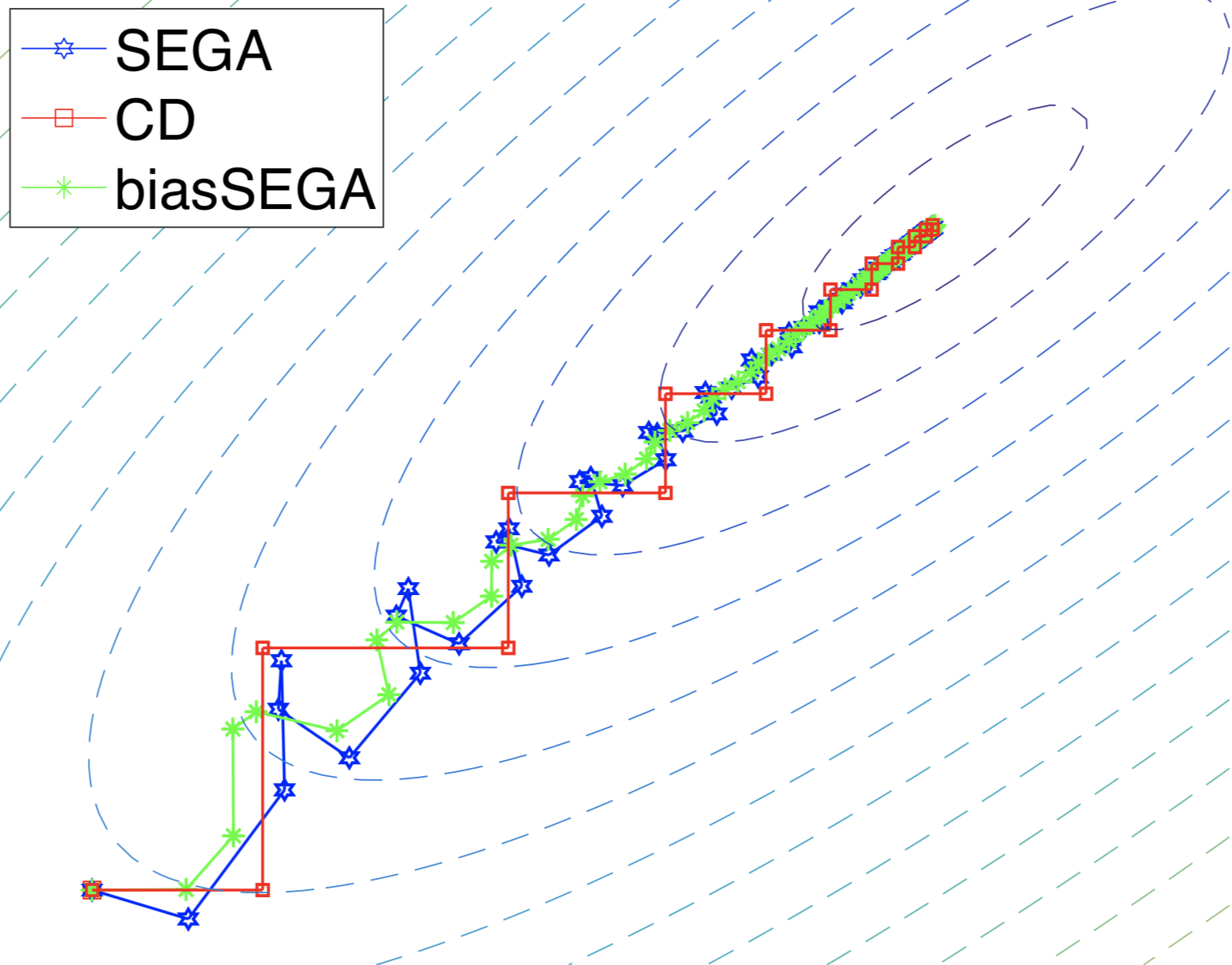
Figure 5: Evolution of iterates of SEGA, CD and biasSEGA (updates made via $h^{k+1}$ instead of $g^{k}$).

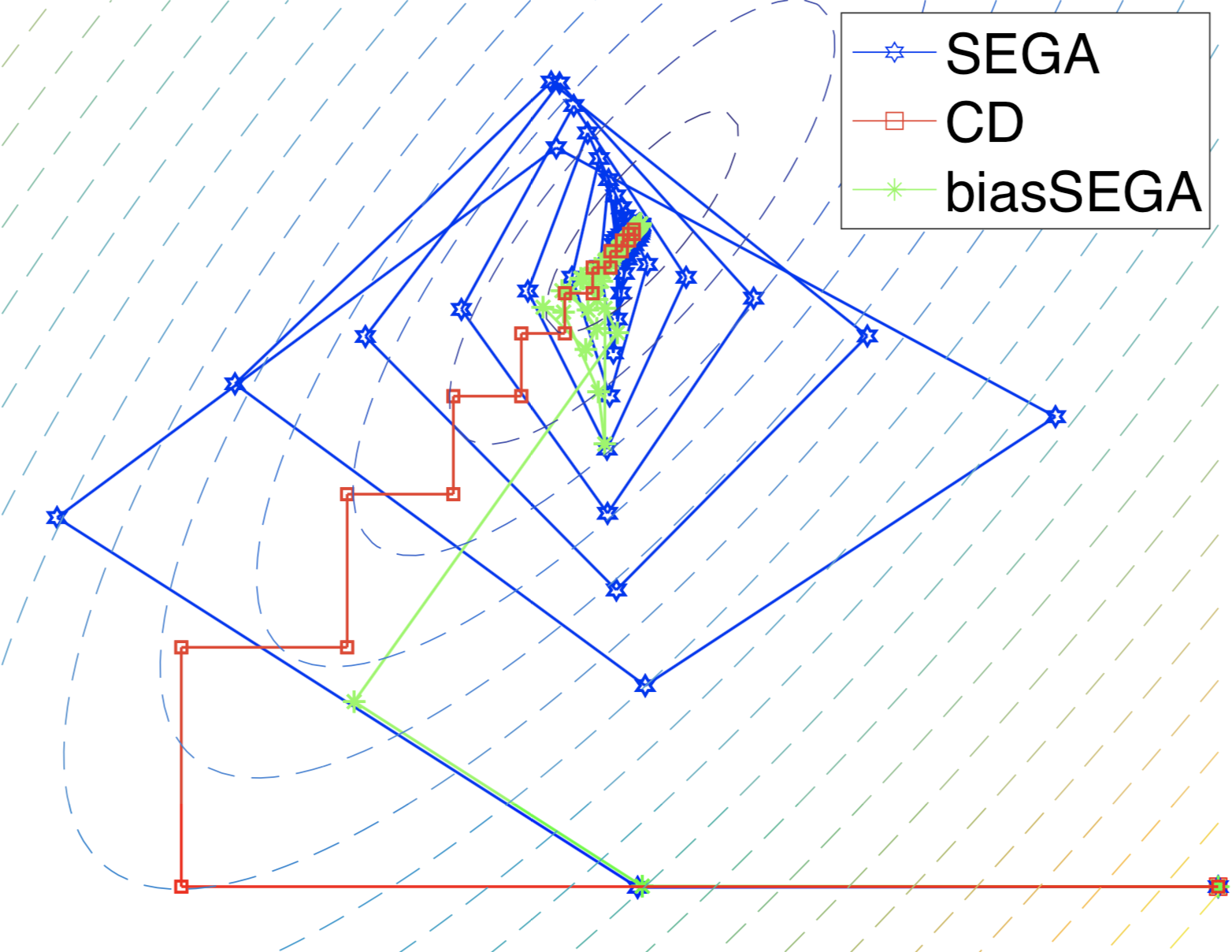
Figure 6: Iterates of SEGA, CD and biasSEGA (updates made via $h^{k+1}$ instead of $g^{k}$). Different starting point.

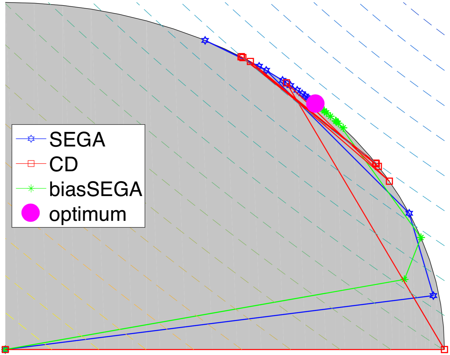
Figure 7: Iterates of projected SEGA, projected CD (which do not converge) and projected biasSEGA (updates made via $h^{k+1}$ instead of $g^{k}$). The constraint set is represented by the shaded region.

F.2 Experiments from Section 5 with empirically optimal stepsize

In the experiments in Section 5, we worked with quadratic functions of the form

$$f(x)\overset{\text{def}}{=}\frac{1}{2}x^{\top}{\bf M}x-b^{\top}x,$$

where $b$ is a random vector with independent entries from ${\cal N}(0,1)$ and ${\bf M}\overset{\text{def}}{=}{\bf U}\Sigma{\bf U}^{\top}$ according to Table 2 for ${\bf U}$ obtained from QR decomposition of random matrix with independent entries from ${\cal N}(0,1)$. For each problem, the starting point was chosen to be a vector with independent entries from ${\cal N}(0,1)$.

Type	$\Sigma$
1	Diagonal matrix with first $n/2$ components equal to 1 and the rest equal to $n$
2	Diagonal matrix with first $n-1$ components equal to 1 and the remaining one equal to $n$
3	Diagonal matrix with $i$–th component equal to $i$
4	Diagonal matrix with components coming from uniform distribution over $[0,1]$

Table 2: Spectrum of ${\bf M}$.

The results are provided in Figures 8-10. They include zeroth-order experiments and the subspace version of SEGA.

Figure 8: Counterpart to Figure 2 – convergence illustration of SEGA and PGD. The indicator “Xn” in the label stands for the setting when the cost of solving linear system is $Xn$ times higher comparing to the oracle call. Recall that a linear system is solved after each $n$ oracle calls. Empirically best stepsizes were used both PGD and SEGA.

Figure 9: Counterpart to Figure 3 – comparison of SEGA and randomized direct search for a various problems. Empirically best stepsizes were used for both methods.

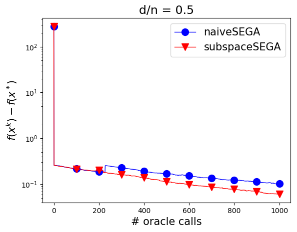
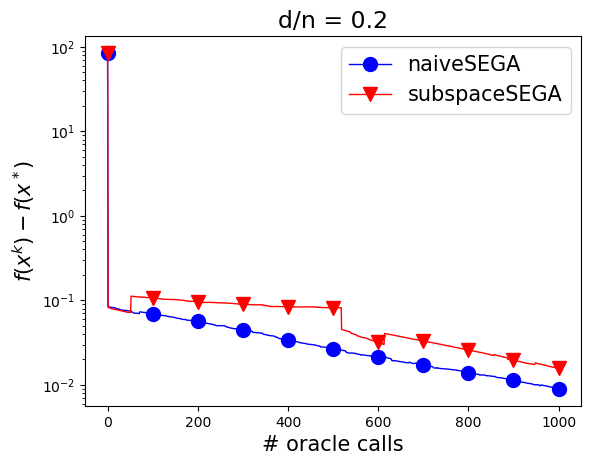
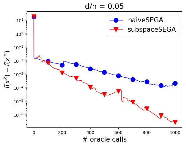
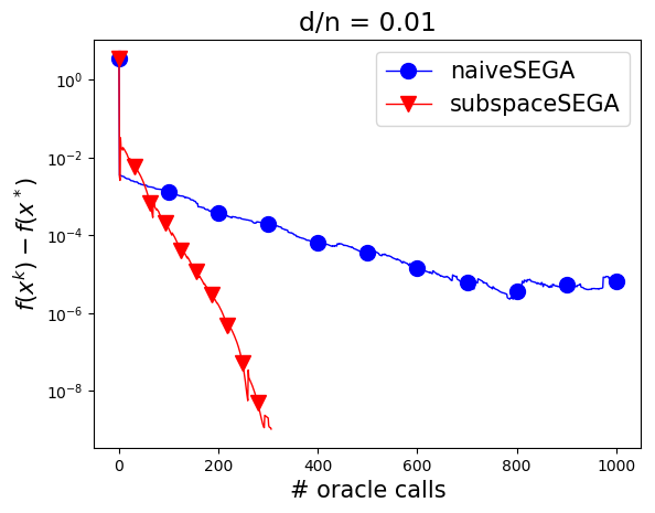
Figure 10: Counterpart to Figure 4 – comparison of SEGA with sketches from a correct subspace versus naive SEGA. Optimal (empirically) stepsize chosen.

F.3 Experiment: comparison with randomized coordinate descent

In this section we numerically compare the results from Section 4 to analogous results for coordinate descent (as indicated in Table 1). We consider the ridge regression problem on LibSVM [7] data, for both primal and dual formulation. For all methods, we have chosen parameters as suggested from theory Figure 11 shows the results. We can see that in all cases, SEGA is slower to the corresponding coordinate descent method, but still is competitive. We however observe only constant times difference in terms of the speed, as suggested by Table 1.

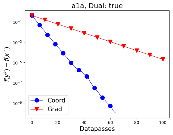
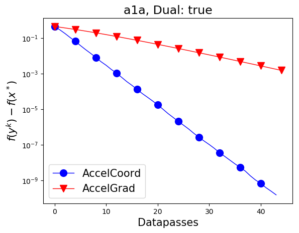
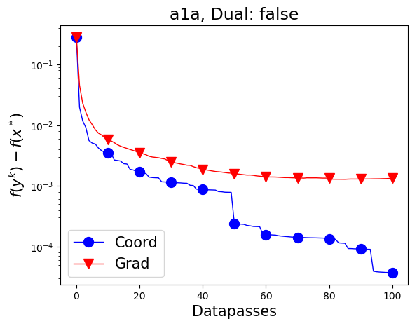
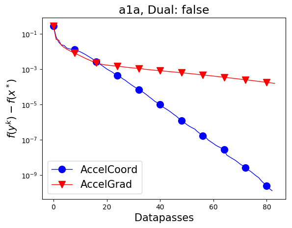
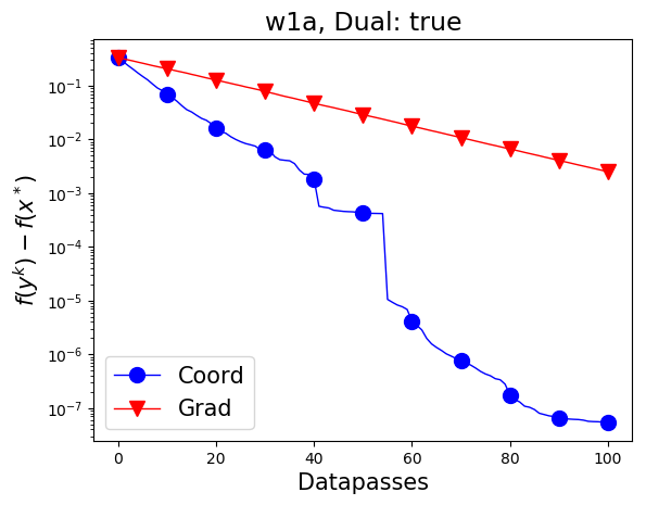
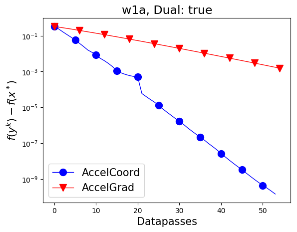
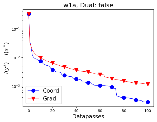
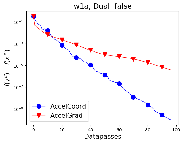
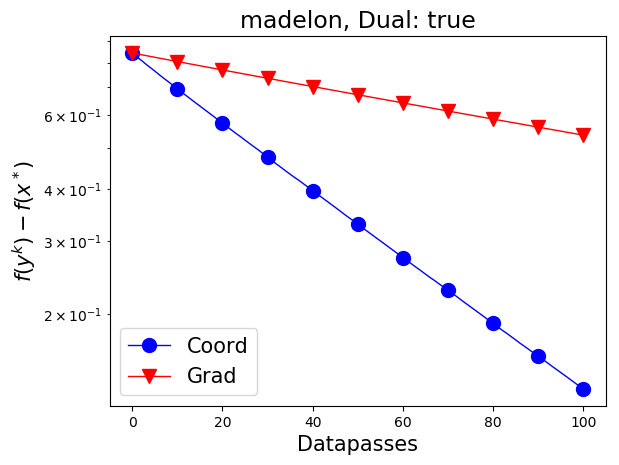
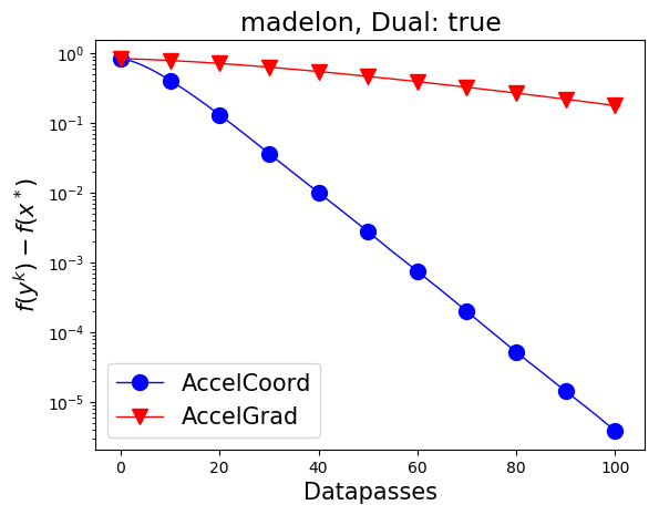
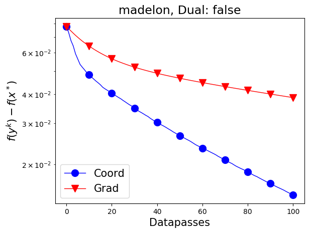
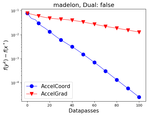
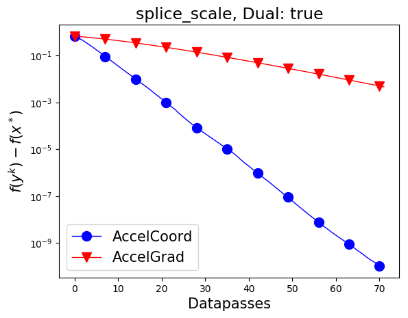
Figure 11: Comparison of SEGA and ASEGA with corresponding coordinate descent methods for $R=0$.

F.4 Experiment: large-scale logistic regression

In this experiment, we set ${\bf B}$ to be identity matrix and compare CD to SEGA with coordinate sketches, both with uniform sampling and with similar stepsizes. The problem considered is logistic regression with $\ell_{2}$ penalty:

$$\min_{x\in\mathbb{R}^{n}}\frac{1}{m}\sum_{i=1}^{m}\log\left(1+\exp(-b_{i}a_{i}^{\top}x)\right)+\frac{\mu}{2}\|x\|_{2}^{2},$$

where $a_{i}$ and $b_{i}$ are data-dependent. Clearly, this regularizer is separable, so we can easily apply both methods. The value of $\mu$ was chosen to be of order $\frac{1}{m}$ in both experiments. Here we use real-world large scale datasets from the LIBSVM [7] library, a summary can be found in Table 3. To make it clear whether CD and SEGA converge with the same speed if given similar stepsizes, we use stepsize $\frac{1}{L}$ for CD and $\frac{1}{dL}$ for SEGA. The results can be found in Figure 12.

Dataset	$m$	$n$	$L$	$\mu$
Epsilon	400000	2000	0.25	$2.5\cdot 10^{-5}$
Covtype	581012	54	21930585. 25	$10^{-1}$

Table 3: Description of the datasets used in our logistic regression experiments. Constants $m$, $n$, $L$ and $\mu$ denote respectively the size of the training set, the number of features, the Lipschitz constant, and the value of $\ell_{2}$ penalty.

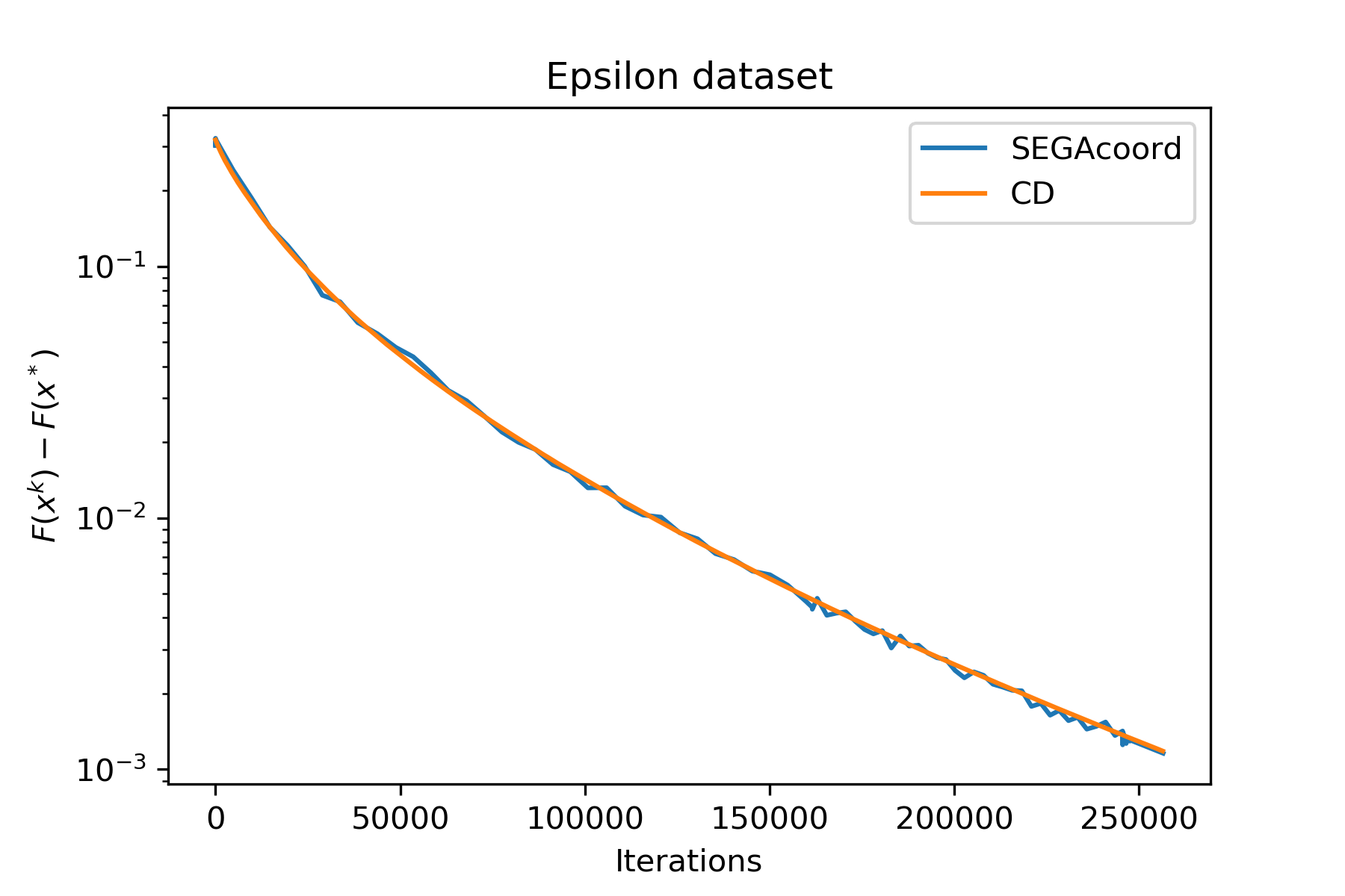
Figure 12: Comparison of SEGA with CD on logistic regression problem with similar stepsizes.

Appendix G Frequently Used Notation

Basic
$\mathbb{E}\left[\cdot\right]$, $\mathbb{P}\left(\cdot\right)$	Expectation / Probability
$\langle\cdot,\cdot\rangle_{\bf B}$, $\|\cdot\|_{\bf B}$	Weighted inner product and norm: $\langle x,y\rangle_{\bf B}=x^{\top}{\bf B}y$; $\|x\|_{\bf B}=\sqrt{\langle x,x\rangle_{\bf B}}$
$e_{i}$	$i$-th vector from the standard basis
${\bf I}$	Identity matrix
$\lambda_{\max}(\cdot),\lambda_{\min}(\cdot)$	Maximal eigenvalue / minimal eigenvalue
$f$	Objective to be minimized over set $\mathbb{R}^{n}$	(1)
$R$	Regularizer	(1)
$x^{*}$	Global optimum
$L$	Lipschitz constant for $\nabla f$
${\bf Q}$	Smoothness matrix	(10)
${\bf M}$	Smoothness matrix, equal to ${\bf Q}^{-1}$ for ${\bf B}={\bf I}$	(11)
$\mu$	Strong convexity constant
SEGA
${\cal D}$	Distribution over sketch matrices $\mathbf{S}$
$\mathbf{S}$	Sketch matrix	(3)
$\mathbb{E}_{{\cal D}}\left[\cdot\right]$	Expectation over the choice of $\mathbf{S}$
$b$	Random variable such that $\mathbf{S}\in\mathbb{R}^{n\times b}$
$\zeta(\mathbf{S},x)$	Sketched gradient at $x$	(2)
${\bf Z}$	$\mathbf{S}\left(\mathbf{S}^{\top}{\bf B}^{-1}\mathbf{S}\right)^{\dagger}\mathbf{S}^{\top}$
$\theta$	Random variable for which $\mathbb{E}_{{\cal D}}\left[\theta{\bf Z}\right]={\bf B}$	(5)
${\bf C}$	$\mathbb{E}_{{\cal D}}\left[\theta^{2}{\bf Z}\right]$	Thm 3.3
$h,g$	Biased and unbiased gradient estimators	(4), (6)
$\alpha$	Stepsize
${\Phi}$	Lyapunov function	Thm 3.3,
$\sigma$	Parameter for Lyapunov function	Thm 3.3, 4.2
Extra Notation for Section 4
$p$, ${{\bf P}}$	Probability vector and matrix
$v$	vector of ESO parameters	(14)
${\bf\hat{P}},{\bf\hat{V}}$	${\rm Diag}(p),{\rm Diag}(v)$
$\gamma$	$\alpha-\alpha^{2}\max_{i}\{\tfrac{v_{i}}{p_{i}}\}-\sigma$	Thm 4.2
$y,z$	Extra sequences of iterates for ASEGA
$\tau,\beta$	Parameters for ASEGA
${\Psi},{\Upsilon}$	Lyapunov functions	Thm 4.2, B.5
${\rm\eta}(v,p)$	$\max_{i}\frac{\sqrt{v_{i}}}{p_{i}}$

Table 4: Summary of frequently used notation.

References

• [1] Zeyuan Allen-Zhu. Katyusha: The first direct acceleration of stochastic gradient methods. In Proceedings of the 49th Annual ACM SIGACT Symposium on Theory of Computing, pages 1200–1205. ACM, 2017.
• [2] Zeyuan Allen-Zhu and Lorenzo Orecchia. Linear coupling: An ultimate unification of gradient and mirror descent. In Innovations in Theoretical Computer Science, 2017.
• [3] Zeyuan Allen-Zhu, Zheng Qu, Peter Richtárik, and Yang Yuan. Even faster accelerated coordinate descent using non-uniform sampling. In Proceedings of The 33rd International Conference on Machine Learning, volume 48 of Proceedings of Machine Learning Research, pages 1110–1119, 2016.
• [4] Amir Beck and Marc Teboulle. A fast iterative shrinkage-thresholding algorithm for linear inverse problems. SIAM Journal on Imaging Sciences, 2(1):183–202, 2009.
• [5] El Houcine Bergou, Peter Richtárik, and Eduard Gorbunov. Random direct search method for minimizing nonconvex, convex and strongly convex functions. Manuscript, 2018.
• [6] Antonin Chambolle, Matthias J. Ehrhardt, Peter Richtárik, and Carola-Bibiane Schöenlieb. Stochastic primal-dual hybrid gradient algorithm with arbitrary sampling and imaging applications. SIAM Journal on Optimization, 28(4):2783–2808, 2018.
• [7] Chih-Chung Chang and Chih-Jen Lin. LibSVM: A library for support vector machines. ACM transactions on intelligent systems and technology (TIST), 2(3):27, 2011.
• [8] Andrew R Conn, Katya Scheinberg, and Luis N Vicente. Introduction to derivative-free optimization, volume 8. Siam, 2009.
• [9] Alexandre d’Aspremont. Smooth optimization with approximate gradient. SIAM Journal on Optimization, 19(3):1171–1183, 2008.
• [10] Aaron Defazio, Francis Bach, and Simon Lacoste-Julien. SAGA: A fast incremental gradient method with support for non-strongly convex composite objectives. In Advances in Neural Information Processing Systems, pages 1646–1654, 2014.
• [11] Olivier Devolder, François Glineur, and Yurii Nesterov. First-order methods of smooth convex optimization with inexact oracle. Mathematical Programming, 146(1-2):37–75, 2014.
• [12] Olivier Fercoq and Peter Richtárik. Accelerated, parallel and proximal coordinate descent. SIAM Journal on Optimization, (25):1997–2023, 2015.
• [13] Robert M Gower, Peter Richtárik, and Francis Bach. Stochastic quasi-gradient methods: Variance reduction via Jacobian sketching. arXiv preprint arXiv:1805.02632, 2018.
• [14] Robert Mansel Gower, Donald Goldfarb, and Peter Richtárik. Stochastic block BFGS: squeezing more curvature out of data. In 33rd International Conference on Machine Learning, pages 1869–1878, 2016.
• [15] Robert Mansel Gower, Filip Hanzely, Peter Richtárik, and Sebastian Stich. Accelerated stochastic matrix inversion: general theory and speeding up BFGS rules for faster second-order optimization. arXiv:1802.04079, 2018.
• [16] Robert Mansel Gower and Peter Richtárik. Randomized iterative methods for linear systems. SIAM Journal on Matrix Analysis and Applications, 36(4):1660–1690, 2015.
• [17] Robert Mansel Gower and Peter Richtárik. Stochastic dual ascent for solving linear systems. arXiv preprint arXiv:1512.06890, 2015.
• [18] Robert Mansel Gower and Peter Richtárik. Linearly convergent randomized iterative methods for computing the pseudoinverse. arXiv:1612.06255, 2016.
• [19] Robert Mansel Gower and Peter Richtárik. Randomized quasi-Newton updates are linearly convergent matrix inversion algorithms. SIAM Journal on Matrix Analysis and Applications, 38(4):1380–1409, 2017.
• [20] Filip Hanzely and Peter Richtárik. Accelerated coordinate descent with arbitrary sampling and best rates for minibatches. arXiv preprint arXiv:1809.09354, 2018.
• [21] Robert Hooke and Terry A Jeeves. “Direct search” solution of numerical and statistical problems. Journal of the ACM (JACM), 8(2):212–229, 1961.
• [22] Rie Johnson and Tong Zhang. Accelerating stochastic gradient descent using predictive variance reduction. In Advances in Neural Information Processing Systems, pages 315–323, 2013.
• [23] Hamed Karimi, Julie Nutini, and Mark Schmidt. Linear convergence of gradient and proximal-gradient methods under the Polyak-Lojasiewicz condition. In Joint European Conference on Machine Learning and Knowledge Discovery in Databases, pages 795–811. Springer, 2016.
• [24] Tamara G Kolda, Robert Michael Lewis, and Virginia Torczon. Optimization by direct search: New perspectives on some classical and modern methods. SIAM Review, 45(3):385–482, 2003.
• [25] Jakub Konečný and Peter Richtárik. Simple complexity analysis of simplified direct search. arXiv preprint arXiv:1410.0390, 2014.
• [26] Hongzhou Lin, Julien Mairal, and Zaid Harchaoui. A universal catalyst for first-order optimization. In Advances in Neural Information Processing Systems, pages 3384–3392, 2015.
• [27] Qihang Lin, Zhaosong Lu, and Lin Xiao. An accelerated proximal coordinate gradient method. In Advances in Neural Information Processing Systems, pages 3059–3067, 2014.
• [28] Nicoas Loizou and Peter Richtárik. Accelerated gossip via stochastic heavy ball method. In 56th Annual Allerton Conference on Communication, Control, and Computing, 2018.
• [29] Nicolas Loizou and Peter Richtárik. A new perspective on randomized gossip algorithms. In IEEE Global Conference on Signal and Information Processing (GlobalSIP), pages 440–444, 2016.
• [30] Nicolas Loizou and Peter Richtárik. Linearly convergent stochastic heavy ball method for minimizing generalization error. In NIPS Workshop on Optimization for Machine Learning, 2017.
• [31] Nicolas Loizou and Peter Richtárik. Momentum and stochastic momentum for stochastic gradient, Newton, proximal point and subspace descent methods. arXiv:1712.09677, 2017.
• [32] Ion Necoara, Peter Richtárik, and Andrei Patrascu. Randomized projection methods for convex feasibility problems: conditioning and convergence rates. arXiv:1801.04873, 2018.
• [33] Yurii Nesterov. A method of solving a convex programming problem with convergence rate ${O}(1/k^{2})$. Soviet Mathematics Doklady, 27(2):372–376, 1983.
• [34] Yurii Nesterov. Introductory lectures on convex optimization: A basic course. Kluwer Academic Publishers, 2004.
• [35] Yurii Nesterov. Smooth minimization of nonsmooth functions. Mathematical Programming, 103:127–152, 2005.
• [36] Yurii Nesterov. Efficiency of coordinate descent methods on huge-scale optimization problems. SIAM Journal on Optimization, 22(2):341–362, 2012.
• [37] Lam M. Nguyen, Jie Liu, Katya Scheinberg, and Martin Takáč. SARAH: A novel method for machine learning problems using stochastic recursive gradient. In Proceedings of the 34th International Conference on Machine Learning, volume 70 of Proceedings of Machine Learning Research, pages 2613–2621. PMLR, 2017.
• [38] Zheng Qu and Peter Richtárik. Coordinate descent with arbitrary sampling I: Algorithms and complexity. Optimization Methods and Software, 31(5):829–857, 2016.
• [39] Zheng Qu and Peter Richtárik. Coordinate descent with arbitrary sampling I: Algorithms and complexity. Optimization Methods and Software, 31(5):829–857, 2016.
• [40] Zheng Qu and Peter Richtárik. Coordinate descent with arbitrary sampling II: Expected separable overapproximation. Optimization Methods and Software, 31(5):858–884, 2016.
• [41] Zheng Qu, Peter Richtárik, Martin Takáč, and Olivier Fercoq. SDNA: Stochastic dual Newton ascent for empirical risk minimization. In Proceedings of The 33rd International Conference on Machine Learning, volume 48 of Proceedings of Machine Learning Research, pages 1823–1832. PMLR, 2016.
• [42] Zheng Qu, Peter Richtárik, and Tong Zhang. Quartz: Randomized dual coordinate ascent with arbitrary sampling. In Advances in Neural Information Processing Systems, pages 865–873, 2015.
• [43] Peter Richtárik and Martin Takáč. On optimal probabilities in stochastic coordinate descent methods. Optimization Letters, 10(6):1233–1243, 2016.
• [44] Peter Richtárik and Martin Takáč. Stochastic reformulations of linear systems: algorithms and convergence theory. arXiv:1706.01108, 2017.
• [45] H. Robbins and S. Monro. A stochastic approximation method. Annals of Mathematical Statistics, 22:400–407, 1951.
• [46] Nicolas Le Roux, Mark Schmidt, and Francis Bach. A stochastic gradient method with an exponential convergence rate for finite training sets. In Advances in Neural Information Processing Systems, pages 2663–2671, 2012.
• [47] Mark Schmidt, Nicolas L Roux, and Francis R Bach. Convergence rates of inexact proximal-gradient methods for convex optimization. In Advances in Neural Information Processing Systems, pages 1458–1466, 2011.
• [48] Shai Shalev-Shwartz and Tong Zhang. Proximal stochastic dual coordinate ascent. arXiv preprint arXiv:1211.2717, 2012.