Variational Inference for Stochastic Control of Infinite Dimensional Systems

Abstract

This paper develops a variational inference framework for control of infinite dimensional stochastic systems. We employ a measure theoretic approach which relies on the generalization of Girsanov’s theorem, as well as the relation between relative entropy and free energy. The derived control scheme is applicable to a large class of stochastic, infinite dimensional systems, and can be used for trajectory optimization and model predictive control. Our work opens up new research avenues at the intersection of stochastic control, inference and information theory for dynamical systems described by stochastic partial differential equations.

1 Introduction

In many practical applications, one faces the problem of controlling dynamical systems represented by stochastic partial differential equations (SPDEs). Examples can be found, for instance, in fluid mechanics, open quantum systems, turbulence, plasma physics and partially observable stochastic control Chow (2007); Da Prato and Zabczyk (2014); Mikulevicius and Rozovskii (2004); G. Dumont and Longtin (2017); Pardouxt (1980); Bang et al. (1994); Cont (2005); Knopf and Weber (2017). Despite the importance of such applications, the majority of works on computational stochastic control has been dedicated to finite dimensional systems. These are systems represented by stochastic differential equations (SDEs), and can be found in a plethora of applications from robotics and autonomous systems, to computational neuroscience, biology and finance. In contrast, the literature is lacking works on scalable/implementable control schemes for stochastic, infinite dimensional systems. To this end, this paper tries to bridge the gap between theory and implementation of stochastic control in infinite dimensions. Our approach is based on the free energy-relative entropy duality, and utilizes elements from stochastic calculus in Hilbert spaces. The resulting methodology avoids restictive assumptions about the problem formulation, and can be applied to a broad class of semilinear SPDEs.

Previous work in the area of control of SPDEs has focused on very specific systems, and typically consists of theoretical results on the existence and uniqueness of solutions. References Prato and Debussche (1999) and Feng (2006) share some common characteristics with our paper. In particular, the former work investigates explicit solutions of the Hamilton-Jacobi-Bellman (HJB) equation for the stochastic Burgers equation. The derivation is based on the exponential transformation of the value function, as well as the transformation of the backward HJB equation into a forward Kolmogorov equation. Then, the explicit solution is recovered through the forward Feynman-Kac lemma and a probabilistic representation of the value function. The work in Feng (2006) extends the large deviation theory to infinite dimensional systems, and creates connections to HJB theory. The analysis therein shows that a free energy-like function corresponds to the value function of a deterministic optimal control problem under a specific cost functional. This connection is established by proving that the aforementioned free energy-like function satisfies the HJB equation of an infinite horizon deterministic optimal control problem.

On the computational side, the work in Lou et al. (2009) proposes a model predictive control methodology for nonlinear dissipative SPDEs. The key idea lies in model reduction; that is, the transformation of the original SPDE into a set of coupled stochastic differential equations. Once this finite dimensional representation is obtained, a model predictive control methodology is developed and is then applied on the Kuramoto-Sivanshisky equation. Another work on computational control of the aforementioned SPDE can be found in Gomes et al. (2017). This approach shares similarities with the one in Lou et al. (2009), in that a finite dimensional representation of the SPDE is utilized, rendering thus the use of standard control theory feasible.

To the best of our knowledge, the framework developed in this paper is the first step towards explicitly designing implementable, numerical stochastic control algorithms in infinite dimensions. In contrast to prior work (see Lou et al. (2009); Gomes et al. (2017)), the proposed approach treats SPDEs as time-indexed stochastic processes taking values in an infinite dimensional space. The core of our methodology relies on sampling stochastic paths from the dynamics, and computing the associated trajectory costs. Grounded on the theory of stochastic calculus in Hilbert spaces, we are not restricted to any particular finite representation of the original system. Besides the theoretical implications, this fact is also benfecial from a computational standpoint. Specifically, the obtained expressions for our control updates are independent of the method used to actually simulate the SPDEs. This further implies that the required sampled paths can be obtained by employing the scheme that is more suitable to each particular problem setup (e.g., finite differences, Galerkin methods or finite elements). Finally, we note that this work can be considered as a generalization of the Path Integral and information theoretic control method Todorov (2009); Theodorou and Todorov (2012); Theodorou (2015); Kappen (2005). As such, the proposed stochastic control algorithm can be efficiently applied in a Model Predictive Control (MPC) fashion, and inherits the ability to deal with non-quadratic cost functions and nonlinear dynamics.

The rest of the paper is organized as follows: In section 2 we provide some important definitions and theorems on infinite dimensional stochastic systems. In section 3 we discuss the free energy and relative entropy relation. Based on this connection, section 4 derives our stochastic control method by performing inference in Hilbert spaces. Furthermore, in subsection 4.1 we develop an iterative version of our framework, which is subsequently tested in simulation in section 5. Section 6 concludes the paper.

2 Preliminaries - Stochastic Calculus

In this paper we consider infinite dimensional stochastic systems of the following form:

$${\mathrm{d}}X={\cal A}X(t){\mathrm{d}}t+F(X(t)){\mathrm{d}}t+G(X(t)){\mathrm{d}}W(t),\quad X(0)=\xi$$ (1)

defined on the probability space $(\Omega,\mathscr{F},\mathbb{P})$ with filtration $\mathscr{F}_{t},t\geq 0$, for the time interval $t\in[0,T]$. Let, $H$ and $U$ Hilbert spaces, then ${\cal A}:D({\cal A})\subset H\to H$ is a infinitesimal generator , $\xi$ is an $\mathscr{F}_{0}-$measurable $H-$valued random variable, while $F:H\to H$ and $G:U\to H$ are nonlinear mappings that satisfy properly formulated Lipschitz and linear growth conditions (associated with the existence and uniqueness of solutions for infinite dimensional stochastic systems - see (Da Prato and Zabczyk, 2014, Theorem 7.2)). The term $W(t)\in U$ corresponds to a $Q$-Wiener process that is defined based on the following proposition (see (Da Prato and Zabczyk, 2014, Chapter 4)). We use the notation $X(\cdot,\omega)$ to denote a state trajectory.

Proposition 2.1.

Let $\{e_{i}\}_{i=1}^{\infty}$ be a complete orthonormal system for the Hilbert Space $U$ such that $Qe_{i}=\lambda_{i}e_{i}$. Here, $\lambda_{i}$ is the eigenvalue of $Q\in L(U)$ that corresponds to eigenvector $e_{i}$, and $L(U)$ denotes the space of linear operators acting on $U$. Then, a $Q$-Wiener process $W(t)\in U$ satisfies the following properties:

1. $W$ is a Gaussian process on $U$ with mean and variance:

   $$\mathbb{E}[W(t)]=0,\quad\mathbb{E}[W(t)W(t)]=tQ,~{}t\geq 0.$$ (2)

2. For arbitrary $t\geq 0$, $W$ has the following expansion:

   $$W(t)=\sum_{j=1}^{\infty}\sqrt{\lambda_{j}}\beta_{j}(t)e_{j},$$ (3)

   where $\beta_{j}(t)$ are real valued brownian motions that are mutually independent on $(\Omega,\mathscr{F},P).$

In this paper we will make use of Girsanov’s theorem for systems evolving on Hilbert spaces. To this end, let us introduce the Hilbert space $U_{0}:=Q^{1/2}(U)\subset U$ with inner product: $\langle u,v\rangle_{U_{0}}:=\langle Q^{-1/2}u,Q^{-1/2}v\rangle_{U}$, $\forall u,v\in U_{0}$. The following proposition is from (Da Prato and Zabczyk, 2014, Theorem 10.18):

Proposition 2.2 (Girsanov).

Let $\Omega$ be a sample space with a $\sigma$-algebra $\mathcal{F}$. Consider the following $H$-valued stochastic processes:

$${\mathrm{d}}X =({\cal A}X+F(X)){\mathrm{d}}t+G(X){\mathrm{d}}W(t),\quad X(0)=x$$ (4)

$${\mathrm{d}}\tilde{X} =({\cal A}\tilde{X}+F(\tilde{X})){\mathrm{d}}t+\tilde{B}(\tilde{X}){\mathrm{d}}t+G(\tilde{X}){\mathrm{d}}W(t),\quad\tilde{X}(0)=x,$$ (5)

where $W\in U$ is a Q-Wiener process with respect to the measure $\mathbb{P}$. Moreover, $\forall\Gamma\in C([0,T];H)$ let the law of $X$ defined as $\mathcal{L}(X(\cdot,\omega)\in\Gamma):=\mathbb{P}(\omega\in\Omega|X(\cdot,\omega)\in\Gamma)$ . Similarly, the law of $\tilde{X}$, is defined as $\tilde{{\mathcal{L}}}(\tilde{X}(\cdot,\omega)\in\Gamma):=\mathbb{P}(\omega\in\Omega|\tilde{X}(\cdot,\omega)\in\Gamma)$. Then

$$\begin{split}&\tilde{{\mathcal{L}}}(\omega)=\mathbb{E}_{\mathbb{P}}\big{[}\exp\big{(}\int_{0}^{T}\langle\psi(s),dW(s)\rangle_{U_{0}}-\frac{1}{2}\int_{0}^{T}||\psi(s)||_{U_{0}}^{2}ds\big{)}|X(\cdot)\in\Gamma\big{]},\end{split}$$ (6)

where $\psi(t):=G^{-1}(X(t))\tilde{B}(X(t))\in U_{0}$. Here, we write for brevity $\tilde{{\mathcal{L}}}(\omega)\equiv\tilde{{\mathcal{L}}}(\tilde{X}(\cdot,\omega)\in\Gamma)$.

Proof.

Define the process:

$$\hat{W}(t):=W(t)-\int_{0}^{t}\psi(s){\mathrm{d}}s.$$ (7)

Based on (Da Prato and Zabczyk, 2014, Theorem 10.18), $\hat{W}$ is a Q-Wiener process with respect to a measure $\mathbb{Q}$ determined by:

$$\begin{split}{\mathrm{d}}\mathbb{Q}(\omega)&=\exp\big{(}\int_{0}^{T}\langle\psi(s),{\mathrm{d}}W(s)\rangle_{U_{0}}-\frac{1}{2}\int_{0}^{T}||\psi(s)||_{U_{0}}^{2}{\mathrm{d}}s\big{)}{\mathrm{d}}\mathbb{P}\\ &=\exp\big{(}\int_{0}^{T}\langle\psi(s),{\mathrm{d}}\hat{W}(s)\rangle_{U_{0}}+\frac{1}{2}\int_{0}^{T}||\psi(s)||_{U_{0}}^{2}{\mathrm{d}}s\big{)}{\mathrm{d}}\mathbb{P}.\end{split}$$ (8)

Now, using (7), eq. (4) is rewritten as:

$$\begin{split}{\mathrm{d}}X&=(AX+F(X)){\mathrm{d}}t+G(X){\mathrm{d}}W(t)=(AX+F(X)){\mathrm{d}}t+B(X){\mathrm{d}}t+G(X){\mathrm{d}}\hat{W}(t)\end{split}$$ (9)

Notice that the above SPDE has the same form as (5). Therefore, under the introduced measure $\mathbb{Q}$, $X$ becomes equivalent to (5). However, under the measure $\mathbb{P}$, the SPDE in (9) behaves as the original system in (4). In other words, eqs. (4) and (9) describe the same system on $(\Omega,\mathcal{F},\mathbb{P})$. From the uniqueness of solutions and the aforementioned reasoning, one has

$$\mathbb{P}(\{\tilde{X}\in\Gamma\})=\mathbb{Q}(\{X\in\Gamma\}).$$

The result follows from (8). ∎

To conclude this section, we note that when $\lambda_{j}=1$, $\forall j$, $W(t)$ corresponds to a cylindrical Wiener process (space-time white noise). In that case, the series in (3) converges in another Hilbert space $U_{1}\supset U$, when the inclusion $\iota:U\rightarrow U_{1}$ is Hilbert-Schmidt. For more details see Da Prato and Zabczyk (2014).

3 Relative Entropy and Free Energy Dualities in Hilbert Spaces

In this section we provide the relation between free energy and relative entropy. The relation is valid for general probability measures including measures defined on path spaces induced by infinite dimensional stochastic systems. Here we will consider the general measures ${\mathcal{L}}$ and $\tilde{{\mathcal{L}}}$.

Definition 3.1.

(Free Energy) Let ${\mathcal{L}}\in\mathscr{P}$ a probability measure and let the function $J\equiv J(X(\cdot,\omega)):L^{p}\to\mathbb{R}_{+}$ be a measurable function. Then the following term:

$$V=\frac{1}{\mu}\log_{e}\int_{\Omega}\exp(\mu J){\mathrm{d}}{\mathcal{L}}(\omega),$$ (10)

is called the free energy of $J$ with respect to ${\mathcal{L}}$ and $\mu\in\mathbb{R}$.

Definition 3.2.

(Generalized Entropy) Let ${\mathcal{L}}\in\mathscr{P}$ and $\tilde{{\mathcal{L}}}\in\mathscr{P}$ then the relative entropy of $\tilde{{\mathcal{L}}}$ with respect to ${\mathcal{L}}$ is defined as:

$$S\left(\tilde{{\mathcal{L}}}||{\mathcal{L}}\ \right)=\left\{\begin{array}[]{l l}-\int_{\Omega}\frac{{\mathrm{d}}\tilde{{\mathcal{L}}}(\omega)}{{\mathrm{d}}{\mathcal{L}}(\omega)}\log_{e}\frac{{\mathrm{d}}\tilde{{\mathcal{L}}}(\omega)}{{\mathrm{d}}{\mathcal{L}}(\omega)}{\mathrm{d}}{\mathcal{L}}(\omega),\mbox{if $\tilde{{\mathcal{L}}}<<{\mathcal{L}}$},\\ +\infty,\quad\mbox{otherwise},\\ \end{array}\right.$$

where “$<<$” denotes absolute continuity of $\tilde{{\mathcal{L}}}$ with respect to ${\mathcal{L}}$ and $\mathcal{L}_{1}$ denotes the space of Lebesgue measurable functions on $[0,\infty)$. We say that $\tilde{{\mathcal{L}}}$ is absolutely continuous with respect to ${\mathcal{L}}$ and we write $\tilde{{\mathcal{L}}}<<{\mathcal{L}}$ if ${\mathcal{L}}(B)=0\Rightarrow\tilde{{\mathcal{L}}}(B)=0,~{}\forall B\in\mathscr{F}$.

The free energy and relative entropy relationship is expressed by the theorem that follows:

Theorem 3.1.

Let $(\Omega,{\mathscr{F}})$ be a measurable space. Consider ${\mathcal{L}},\tilde{{\mathcal{L}}}\in\mathscr{P}$ and the definitions of free energy and relative entropy as expressed in definitions 3.1 and 3.2. Under the assumption that $\mathbb{Q}_{\mathbb{X}}<<\mathbb{P}_{\mathbb{X}}$, the following inequality holds:

$$-\frac{1}{\rho}\log_{e}\mathbb{E}_{{\mathcal{L}}}\bigg{[}\exp(-\rho{J})\bigg{]}\leq\bigg{[}\mathbb{E}_{\tilde{{\mathcal{L}}}}\left({J}\right)-\frac{1}{\rho}S\left(\tilde{{\mathcal{L}}}||{\mathcal{L}}\right)\bigg{]},$$ (11)

where $\mathbb{E}_{{\mathcal{L}}},\mathbb{E}_{\tilde{{\mathcal{L}}}}$ is the expectation under the probability measure ${\mathcal{L}},\tilde{{\mathcal{L}}}$ respectively and $\rho\in\mathbb{R}_{+}$ and $J:L^{p}\to\mathbb{R}_{+}$. The inequality in (11) is the so called Legendre Transform.

By defining the free energy as temperature $T=\frac{1}{\rho}$ the Legendre transformation has the form:

$$V\leq E-TS,$$ (12)

which has statistical mechanics interpretation. The equilibrium probability measure has the classical form:

$${\mathrm{d}}{\mathcal{L}}^{*}(\omega)=\frac{\exp(-\rho J){\mathrm{d}}{\mathcal{L}}(\omega)}{\int_{\Omega}\exp(-\rho J){\mathrm{d}}{\mathcal{L}}(\omega)},$$ (13)

To verify that the measure in (13) is the optimal measure it suffices to substitute (13) in (11) and show that the inequality collapses to an equality Theodorou (2015). The statistical physics interpretation of inequality (12) is that, maximization of entropy results in reduction of the available energy. At the thermodynamic equilibrium the entropy reaches its maximum and the inequality collapses to equality. It can be shown that when the measures $\tilde{{\mathcal{L}}}$ and ${\mathcal{L}}$ are associated to paths generated by control and uncontrolled semi-linear SPDEs, then the free energy is value function that satisfies the HJB equation of an infinite dimensional stochastic optimal control problem. This observation motivates the use of (13) for the development of stochastic control algorithms.

4 Variational Inference and Control in Hilbert Spaces

In this section we will derive our numerical algorithm for controlling stochastic infinite dimensional systems.To simplify our expressions, we will consider without loss of generality SPDEs with additive noise. Let the uncontrolled and controlled version of an $H$-valued process be given respectively by:

$${\mathrm{d}}X(t)=(\mathscr{A}X+F(X(t))){\mathrm{d}}t+\frac{1}{\sqrt{\rho}}{\mathrm{d}}W(t),~{}\text{and}~{}{\mathrm{d}}\tilde{X}(t)=(\mathscr{A}\tilde{X}+F(\tilde{X}(t))+{\cal U}(t)){\mathrm{d}}t+\frac{1}{\sqrt{\rho}}{\mathrm{d}}W(t)$$ (14)

both with initial condition: $X(0)=\tilde{X}(0)=\xi$. Here, $W\in U=H$ is a $Q$-Wiener process on $(\Omega,\mathcal{F},\mathbb{P})$ with covariance operator $Q\in L(U)$. As in the previous section, the uncontrolled dynamics are equivalent to:

$${\mathrm{d}}X(t)=(\mathscr{A}X+F(X(t))+{\cal U}(t)){\mathrm{d}}t+\frac{1}{\sqrt{\rho}}{\mathrm{d}}\hat{W}(t),$$ (15)

with respect to $\mathbb{P}$. Here, $\hat{W}$ is a $Q$-Wiener process with respect to another measure $\mathbb{Q}$. The law of the uncontrolled states, $\mathcal{L}(\cdot)$, defines a measure on the path space via (14) as $\mathcal{L}(\omega):=\mathbb{P}(\omega|X(\cdot,\omega)\in\Gamma)$. Similarly, the law of controlled trajectories is $\tilde{\mathcal{L}}(\omega):=\mathbb{P}(\omega|\tilde{X}(\cdot,\omega)\in\Gamma)$. Finally, we suppose that there exists an optimal controller ${\cal U}^{*}$ which corresponds to the law of optimal trajectories, $\mathcal{L}^{*}(\cdot)$.

In this section we derive controllers by formulating a new optimization problem in which we make use of the measure theoretic approach. We are looking for a control input ${\cal U}(\cdot)$ that minimizes the distance to the optimal path law. That is:

$${\cal U}^{*}(\cdot)=\operatornamewithlimits{argmax}_{{\cal U}(\cdot)}S(\mathcal{L}^{*}||\tilde{\mathcal{L}}).$$ (16)

Under the parameterization ${\cal U}={\cal U}(X(t);{\mbox{\boldmath$\theta$}})$ the problem above will take the form:

$${\mbox{\boldmath$\theta$}}^{*}=\operatornamewithlimits{argmax}\bigg{[}-\int_{\Omega}\frac{{\mathrm{d}}{\mathcal{L}}^{*}(\omega)}{{\mathrm{d}}\tilde{{\mathcal{L}}}(\omega)}\log_{e}\frac{{\mathrm{d}}{\mathcal{L}}^{*}(\omega)}{{\mathrm{d}}\tilde{{\mathcal{L}}}(\omega)}{\mathrm{d}}\tilde{{\mathcal{L}}}(\omega)\bigg{]}=\operatornamewithlimits{argmin}\bigg{[}\int_{\Omega}\ \log_{e}\frac{{\mathrm{d}}{\mathcal{L}}^{*}(\omega)}{{\mathrm{d}}\tilde{{\mathcal{L}}}(\omega)}{\mathrm{d}}{\mathcal{L}}^{*}(\omega)\bigg{]}.$$

To perform the optimization we will consider the chain rule property for the Radon-Nikodym derivative.For instance, this results in the following expression:

$$\frac{{\mathrm{d}}{\mathcal{L}}^{*}(\omega)}{{\mathrm{d}}\tilde{{\mathcal{L}}}(\omega)}=\frac{{\mathrm{d}}{\mathcal{L}}^{*}(\omega)}{{\mathrm{d}}{\mathcal{L}}(\omega)}\frac{{\mathrm{d}}{\mathcal{L}}(\omega)}{{\mathrm{d}}\tilde{{\mathcal{L}}}(\omega)}.$$ (17)

Note that the first derivative is given by (13) while the second derivative is given by the change of measure between control and uncontrolled infinite dimensional stochastic dynamics. Based on the discussion of the previous section, $\tilde{\mathcal{L}}(\omega)=\mathbb{Q}(\omega|X(\cdot,\omega)\in\Gamma)$ and $\mathcal{L}^{*}(\omega)=\mathbb{Q}^{*}(\omega|X(\cdot,\omega)\in\Gamma)$, where $\mathbb{Q}^{*}$ is properly defined. From Proposition 2.2, this is computed by

$$\frac{{\mathrm{d}}\tilde{{\mathcal{L}}}}{{\mathrm{d}}{\mathcal{L}}}=\frac{{\mathrm{d}}\mathbb{Q}}{{\mathrm{d}}\mathbb{P}}=\exp\bigg{(}\int_{0}^{T}\langle\psi(s),{\mathrm{d}}W(s)\rangle_{U_{0}}-\frac{1}{2}\int_{0}^{T}||\psi(s)||_{U_{0}}^{2}{\mathrm{d}}s\bigg{)},$$ (18)

where $\psi(t):=\sqrt{\rho}\mathcal{U}(t)\in U$. In this paper we will parameterize our infinite dimensional control as follows:

$${\cal U}(t)=\sum_{\ell=1}^{N}m_{\ell}u_{\ell}(t)\in U\equiv H,$$ (19)

so that

$${\cal U}(t)({\bf x})=\sum_{\ell=1}^{N}m_{\ell}({\bf x})u_{\ell}(t)={\bf m}({\bf x})^{{\mathrm{T}}}{\bf u}(t)\in\mathbb{R}.$$ (20)

Here, $m_{\ell}\in U$ are design functions that specify how the actuation is incorporated into the infinite dimensional dynamical system. Under this parameterization, the change of measure between the two SPDEs takes the form:

$$\begin{split}\frac{{\mathrm{d}}\mathbb{Q}}{{\mathrm{d}}\mathbb{P}}=\exp\bigg{(}\sqrt{\rho}\int_{0}^{T}{\bf u}(t)^{\top}\bar{{\bf m}}(t)-\rho\frac{1}{2}\int_{0}^{T}{\bf u}(t)^{\top}{\bf M}{\bf u}(t){\mathrm{d}}t\bigg{)},\end{split}$$ (21)

where

$$\bar{{\bf m}}(t):=\bigg{[}\langle m_{1},{\mathrm{d}}W(t)\rangle_{U_{0}},...,\langle m_{N},{\mathrm{d}}W(t)\rangle_{U_{0}}\bigg{]}^{\top}\in\mathbb{R}^{N},$$ (22)

$${\bf M}\in\mathbb{R}^{N\times N},\quad({\bf M})_{ij}:=\langle m_{i},m_{j}\rangle_{U_{0}}.$$ (23)

The following theorem provides the optimal control ${\bf u}^{*}$ for the case of the controlled SPDEs of the form in (14).

Lemma 4.1.

(Variational Stochastic Control) Consider the controlled SPDE in (14) and let the following objective function:

$${\bf u}^{*}=\operatornamewithlimits{argmax}S({\mathcal{L}}^{*}||\tilde{{\mathcal{L}}})$$ (24)

The probability measure ${\mathcal{L}}^{*}$ is induced by the optimally controlled SPDE in (14) and has the form:

$${\mathrm{d}}{\mathcal{L}}^{*}(\omega)=\frac{\exp(-\rho J(Xq)){\mathrm{d}}{\mathcal{L}}(\omega)}{\int_{\Omega}\exp(-\rho J(X)){\mathrm{d}}{\mathcal{L}}(\omega)},$$ (25)

The probability measure $\tilde{{\mathcal{L}}}$ is induced by controlled trajectories of the SPDEs when infinite dimensional control ${\cal U}(t)$ is determined by (26) and ${\bf u}(t)$ in (20) is parameterized as follows:

$${\bf u}(t)={\bf u}_{i}\equiv{\bf u}(t_{i})\quad\text{if }\quad i\Delta t\leq t<(i+1)\Delta t,\quad\forall t\in[0,T]$$ (26)

with $i=\{0,1,\ldots L\}$. Under the aforementioned representation, the optimal control is provided by the following expression:

$${\bf u}^{*}_{i}=\frac{1}{\sqrt{\rho}\Delta t}{\bf M}^{-1}\mathbb{E}_{{\mathcal{L}}}\bigg{[}\frac{\exp(-\rho J)}{\mathbb{E}_{{\mathcal{L}}}[\exp(-\rho J)]}\delta{\bf u}_{i}\bigg{]},\quad\text{and}\quad\delta{\bf u}_{i}:=\int_{t_{i}}^{t_{i+1}}\bar{{\bf m}}(t).$$ (27)

Proof.

Under the parameterization ${\cal U}({\bf x},t)={\bf m}({\bf x})^{{\mathrm{T}}}{\bf u}(t)$ the problem above will take the form:

$${\bf u}^{*}=\operatornamewithlimits{argmin}\bigg{[}\int_{\Omega}\ \log_{e}\frac{{\mathrm{d}}{\mathcal{L}}^{*}(\omega)}{{\mathrm{d}}\tilde{{\mathcal{L}}}(\omega)}{\mathrm{d}}{\mathcal{L}}^{*}(\omega)\bigg{]} =\operatornamewithlimits{argmin}\bigg{[}\int_{\Omega}\ \log_{e}\frac{{\mathrm{d}}{\mathcal{L}}^{*}(\omega)}{{\mathrm{d}}{\mathcal{L}}(\omega)}\frac{{\mathrm{d}}{\mathcal{L}}(\omega)}{{\mathrm{d}}\tilde{{\mathcal{L}}}(\omega)}{\mathrm{d}}{\mathcal{L}}^{*}(\omega)\bigg{]}.$$

By using (21) minimization of the last expression is equivalent to the minimization of the expression:

$$\mathbb{E}_{{\mathcal{L}}^{*}}\bigg{[}\log_{e}\frac{{\mathrm{d}}{\mathcal{L}}(\omega)}{{\mathrm{d}}\tilde{{\mathcal{L}}}(\omega)}\bigg{]} =-\sqrt{\rho}\mathbb{E}_{{\mathcal{L}}^{*}}\bigg{[}\int_{0}^{T}{\bf u}(t)^{\top}\bar{{\bf m}}(t)\bigg{]}+\frac{1}{2}\rho\mathbb{E}_{{\mathcal{L}}^{*}}\bigg{[}\int_{0}^{T}{\bf u}(t)^{\top}{\bf M}{\bf u}(t){\mathrm{d}}t\bigg{]}.$$

The goal is to find the function ${\bf u}^{*}(\cdot)$ which minimizes. However, since we inevitably apply the control in discrete time it suffices to consider the class of step functions:

$$\mathbb{E}_{{\mathcal{L}}^{*}}\bigg{[}\log_{e}\frac{{\mathrm{d}}{\mathcal{L}}(\omega)}{{\mathrm{d}}\tilde{{\mathcal{L}}}(\omega)}\bigg{]}=-\sqrt{\rho}\sum_{i=0}^{L-1}{\bf u}_{i}^{\top}\mathbb{E}_{{\mathcal{L}}^{*}}\bigg{[}\int_{t_{i}}^{t_{i+1}}\bar{{\bf m}}(t)\bigg{]}+\frac{1}{2}\rho\sum_{i=0}^{L-1}{\bf u}_{i}^{\top}{\bf M}{\bf u}_{i}\Delta t,$$

where we have used the fact that ${\bf M}$ is symmetric and constant with respect to time. Minimization of the expression above with respect to ${\bf u}_{i}$ results in:

$${\bf u}_{i}^{*}=\frac{1}{\sqrt{\rho}\Delta t}{\bf M}^{-1}\mathbb{E}_{{\mathcal{L}}^{*}}\bigg{[}\int_{t_{i}}^{t_{i+1}}\bar{{\bf m}}(t)\bigg{]}.$$ (28)

Since we cannot sample from the ${\mathcal{L}}^{*}$, we need to change the expectation to be an expectation with respect to the uncontrolled dynamics, ${\mathcal{L}}$. We can then directly sample trajectories from ${\mathcal{L}}$ to approximate the controls. The change in expectation is achieved by applying the Radon-Nikodym derivative. The result is equation (27). ∎

4.1 Iterative Control of SPDEs

We derive an iterative scheme that can be used for stochastic optimization and be implemented in a receding horizon fashion. In particular, let us consider the controlled dynamics at iteration $i^{th}$ given by:

$${\mathrm{d}}X^{(i)}(t)=(\mathscr{A}X^{(i)}+F(X^{(i)})+{\cal U}^{(i)}(t)){\mathrm{d}}t+\frac{1}{\sqrt{\rho}}{\mathrm{d}}W(t),$$ (29)

where ${\cal U}^{i}(t)$ is the control at the $i^{th}$ iteration. As we have already shown, the uncontrolled dynamics can be equivalently written as:

$$\begin{split}{\mathrm{d}}X(t)&=(\mathscr{A}X+F(X(t))){\mathrm{d}}t+\frac{1}{\sqrt{\rho}}{\mathrm{d}}W(t)=(\mathscr{A}h+F(X(t))+{\cal U}^{(i)}(t)){\mathrm{d}}t+\frac{1}{\sqrt{\rho}}{\mathrm{d}}W^{(i)}(t),\end{split}$$ (30)

where $W^{(i)}$ is a $Q$-Wiener process with respect to some measure $\mathbb{Q}^{(i)}$ with:

$$W^{(i)}(t):=W(t)-\int_{0}^{t}\rho{\cal U}^{(i)}(s){\mathrm{d}}s,$$ (31)

Again here we define the path measure ${\mathcal{L}}^{i}(\omega):=\mathbb{P}(\omega|X^{(i)}(\cdot,\omega)\in\Gamma)$ induced by 29 and the path measure ${\mathcal{L}}(\omega):=\mathbb{P}(\omega|X(\cdot,\omega)\in\Gamma)$ induced by (30). Then according to 2.2 we have:

$$\begin{split}\frac{{\mathrm{d}}\mathbb{{\mathcal{L}}}^{(i)}}{{\mathrm{d}}{\mathcal{L}}}=\frac{{\mathrm{d}}\mathbb{Q}^{(i)}}{{\mathrm{d}}\mathbb{P}}=\exp\big{(}\sqrt{\rho}\sum_{k=0}^{L-1}{\bf u}_{k}^{(i)\top}\int_{t_{k}}^{t_{k+1}}\bar{{\bf m}}^{(i)}(t)+\rho\frac{1}{2}\sum_{k=0}^{L-1}{\bf u}_{k}^{(i)\top}{\bf M}{\bf u}_{k}^{(i)}\Delta t\big{)},\end{split}$$ (32)

where

$$\mathbb{R}^{N}\ni\bar{{\bf m}}^{(i)}(t):=\bigg{[}\langle m_{1},{\mathrm{d}}W^{(i)}(t)\rangle_{U_{0}},...,\langle m_{N},{\mathrm{d}}W^{(i)}(t)\rangle_{U_{0}}\bigg{]}^{\top},$$ (33)

Lemma 4.2.

(Iterative Stochastic Control) Consider the controlled SPDE in (14) and the parameterization of the control as specified by (20) and (26). The iterative control scheme is given by the following expression:

$${\bf u}^{*}_{j}{}^{(i+1)}={\bf u}^{*}_{j}{}^{(i)}+\frac{1}{\sqrt{\rho}\Delta t}{\bf M}^{-1}\mathbb{E}_{{\mathcal{L}}^{(i)}}\bigg{[}\frac{\exp(-\rho\tilde{J})}{\mathbb{E}_{{\mathcal{L}}^{(i)}}[\exp(-\rho\tilde{J}]}\delta{\bf u}^{(i)}_{j}\bigg{]},\quad and\quad\delta{\bf u}^{(i)}_{j}=\int_{t_{j}}^{t_{j+1}}\bar{{\bf m}}^{(i)}(t).$$ (34)

and

$$\tilde{J}=J+\zeta,$$ (35)

with the control path dependent function $\zeta^{(i)}=\zeta({\cal U}^{(i)}):[0,T]\times{\cal O}\to\mathbb{R}$ defined as follows:

$$\zeta({\cal U}^{(i)})= \frac{1}{\sqrt{\rho}}\sum_{k=0}^{L-1}{\bf u}_{k}^{(i)\top}\int_{t_{k}}^{t_{k+1}}\bar{{\bf m}}^{(i)}(t)+\frac{1}{2}\sum_{k=0}^{L-1}{\bf u}_{k}^{(i)\top}{\bf M}{\bf u}_{k}^{(i)}\Delta t.$$ (36)

The expectation in (34) is taken with respect to the probability path measure ${\mathcal{L}}^{(i)}$ induced by sampled trajectories generated using (29).

Proof.

In order to derive the iterative scheme, we perform one step of importance sampling. In particular, instead of sampling from the uncontrolled SPDE (14) to evaluate the expectation in (27) we sample using the controlled SPDE (29). In addition, we modify (27) so that to perform the appropriate change of measure between the uncontrolled version of infinite dimensional dynamics and the controlled version at iteration $i$. Next we modify equations (27) by considering (32) and (31).

$${\bf u}^{(i+1)}_{j}=\frac{1}{\sqrt{\rho}\Delta t}{\bf M}^{-1}\mathbb{E}_{{\mathcal{L}}^{(i)}}\bigg{[}\frac{{\mathrm{d}}{\mathcal{L}}}{{\mathrm{d}}{\mathcal{L}}^{(i)}}\frac{\exp(-\rho J)}{\mathbb{E}_{{\mathcal{L}}}[\exp(-\rho J)]}\delta{\bf u}_{j}\bigg{]},$$ (37)

Regarding $\delta{\bf u}_{j}$, one has:

$$\begin{split}&\bigg{(}\int_{t_{j}}^{t_{j+1}}\bar{{\bf m}}(t)\bigg{)}_{l}=\int_{t_{j}}^{t_{j+1}}\langle m_{l},{\mathrm{d}}W(t)\rangle_{U_{0}}=\\ &\int_{t_{j}}^{t_{j+1}}\langle m_{l},{\mathrm{d}}W^{(i)}(t)+\sqrt{\rho}{\cal U}^{(i)}(t){\mathrm{d}}t\rangle_{U_{0}}=\int_{t_{j}}^{t_{j+1}}\langle m_{l},{\mathrm{d}}W^{(i)}(t)\rangle_{U_{0}}+\sqrt{\rho}\bigg{[}\langle m_{l},m_{1}\rangle_{U_{0}},...,\langle m_{l},m_{N}\rangle_{U_{0}}\bigg{]}{\bf u}_{j}^{(i)}\Delta t.\end{split}$$

It follows that:

$$\int_{t_{j}}^{t_{j+1}}\bar{{\bf m}}(t)=\int_{t_{j}}^{t_{j+1}}\bar{{\bf m}}^{(i)}(t)+\sqrt{\rho}\Delta t{\bf M}{\bf u}_{j}^{(i)}.$$

Substitution of the Radon-Nikodym derivative yields the final result in (34). Note that under $\mathbb{Q}^{(i)}$ renders $W^{(i)}$ a standard $Q$-Wiener process. ∎

For the purposes of implementation we will approximate the optimal controls (34) as:

$$(\delta\tilde{{\bf u}}^{(i)}_{j})_{l}:=\sum_{s=1}^{R}\langle m_{l},\sqrt{\lambda}_{s}e_{s}\rangle_{U_{0}}\Delta\beta^{(i)}_{s}(t_{j}),$$ (38)

where $\Delta\beta^{(i)}_{s}(t_{j})\sim\mathcal{N}(0,\Delta t)$ under $\mathbb{Q}^{(i)}$. Next we discuss the application of the iterative stochastic control on two examples of SPDEs.

5 Experiments

In this section, we present simulation results on two infinite dimensional stochastic systems. The first systems is the stochastic Heat equation and the second system is the Nagumo SPDE. The iterative stochastic optimal control is used for open loop trajectory optimization and for MPC.
Heat SPDE: The 1-D stochastic heat equation with homogeneous Dirichlet boundary conditions can be used to simulate the diffusion of heat along a rod insulated on the sides and exposed to freezing conditions at the end points. Our experiments consisted of achieving desired temperature levels at specific positions along a rod in the presence of space-time stochastic disturbing forces. As seen in Fig. 1, the MPC has robust performance compared to open-loop controller with the mean temperature profile closer to the desired temperature levels and tighter sigma bounds in the presence of space-time white noise.

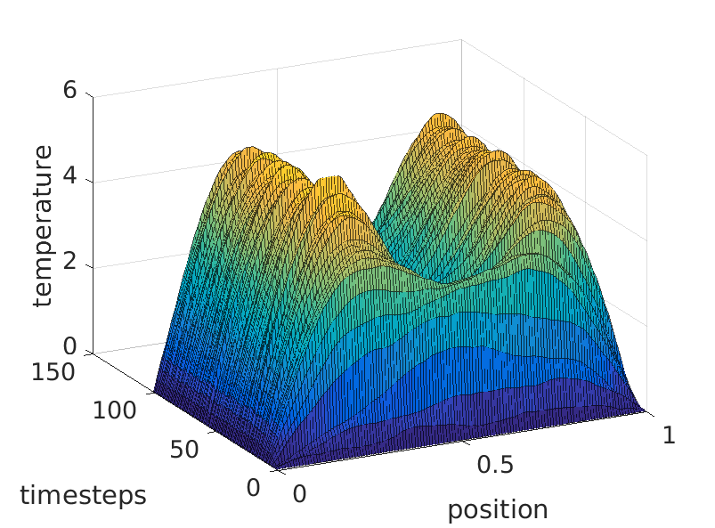
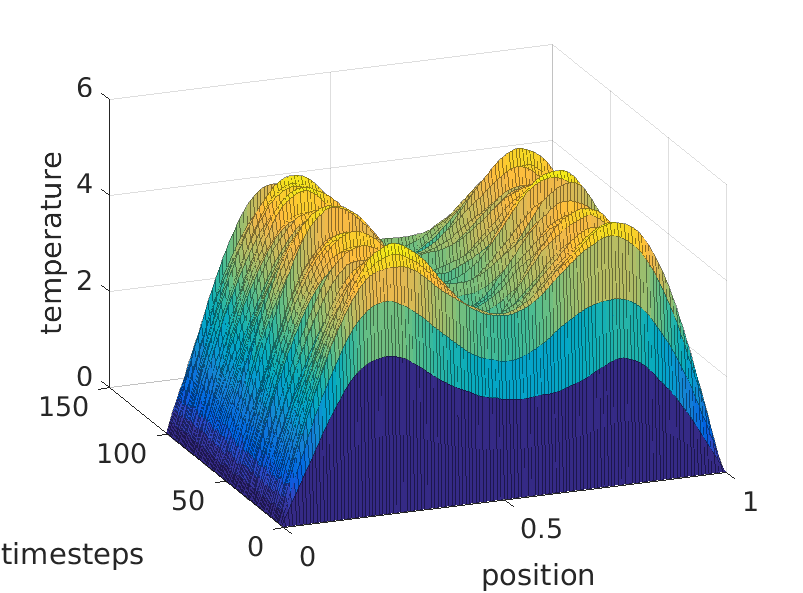
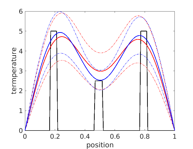
Figure 1: Plots showing the evolution of temperature profile along a rod for Model Predictive Controller (left), Open-Loop controller (middle) and the mean temperature profile for both controllers over an episode within $\pm$1-$\sigma$ bounds (right). Curves in red record performance of open-loop controller, those in blue record MPC. Black bars indicate desired temperature levels.

Nagumo SPDE: The stochastic Nagumo equation with homogeneous Neumann boundary conditions is a reduced model for wave propagation of the voltage $u$ in the axon of a neuron Lord et al. (2014). The Nagumo equation is expressed as follows:

$$u_{t}=\epsilon u_{xx}+u(1-u)(u-\alpha)+\sigma dW(t),\quad u_{x}(t,0)=u_{x}(t,a)=0,u(0,x)=(1+\exp(-(2-x)/\sqrt[]{2}))^{-1}$$

The parameter $\alpha$ determines the speed of a wave traveling down the length of the axon and $\epsilon$ the rate of diffusion. From simulating the deterministic version of the above pde for $a=10,\,\epsilon=1$ and $\alpha=-0.5$, we observed that it requires about 10 seconds for the wave to propagate to the end of the axon An open-loop infinite-dimensional controller was employed to accelerate the propagation of the voltage and to suppress the propagation of the voltage in about 2.5 seconds. The plots shown in the figure below demonstrate the achievement of desired behavior in the axon.

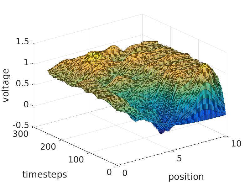
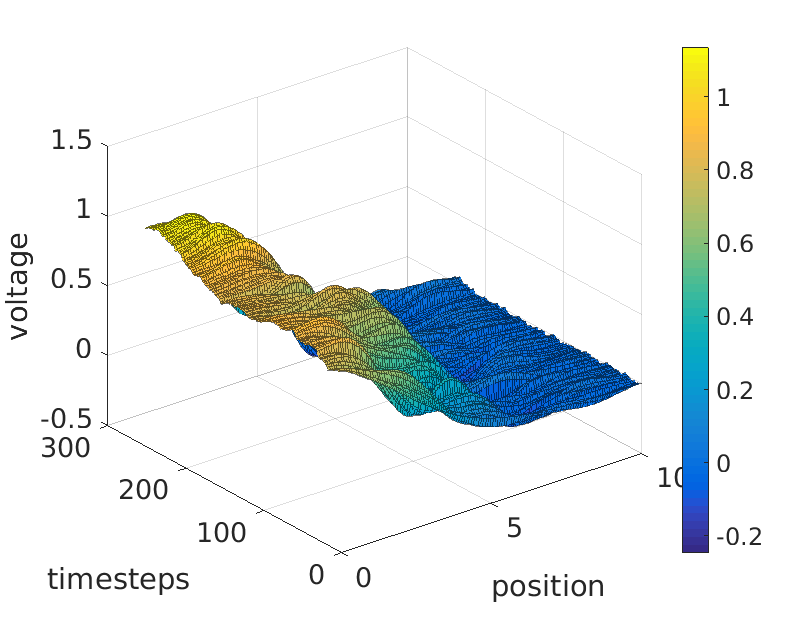
Figure 2: Plots showing the acceleration of voltage propagation in an axon (left) and suppression of voltage propagation in an axon (right)

.

6 Conclusions

We present an information theoretic formulation for stochastic optimal control of infinite dimensional dynamical systems. The analysis relies on concepts drawn from the theory of stochastic calculus in Hilbert spaces, the relative entropy and free energy relation and its connections to stochastic dynamic programming. The resulting algorithm can be used for stochastic trajectory optimization and MPC for a large class of systems with dynamics governed by SPDEs. The work in this paper is a generalization of the path integral and information theoretic control to infinite dimensional spaces and is a significant step towards the development of scalable and real time control algorithms for infinite dimensional stochastic systems. Future directions involve, the theoretical analysis of the convergence, application to higher order infinite dimensional systems, fully nonlinear SPDEs and application to real systems.

References

- Chow [2007] P.L. Chow. Stochastic Partial Differential Equations. Advances in Applied Mathematics. Taylor & Francis, 2007. ISBN 9781584884439. URL https://books.google.com/books?id=x9Ois68HJ0QC.
- Da Prato and Zabczyk [2014] G. Da Prato and J. Zabczyk. Stochastic Equations in Infinite Dimensions. Encyclopedia of Mathematics and its Applications. Cambridge University Press, 2014. ISBN 9780521385299. URL https://books.google.com/books?id=Sid6pwAACAAJ.
- Mikulevicius and Rozovskii [2004] R. Mikulevicius and B. L. Rozovskii. Stochastic navier–stokes equations for turbulent flows. SIAM Journal on Mathematical Analysis, 35(5):1250–1310, 2004.
- G. Dumont and Longtin [2017] A. Payeur. G. Dumont and A. Longtin. A stochastic-field description of finite-size spiking neural networks. PLOS Computational Biology, 13, 08 2017.
- Pardouxt [1980] E. Pardouxt. Stochastic partial differential equations and filtering of diffusion processes. Stochastics, 3(1-4):127–167, 1980.
- Bang et al. [1994] O. Bang, P. L. Christiansen, F. If, K. Ø. Rasmussen, and Y. B. Gaididei. Temperature effects in a nonlinear model of monolayer scheibe aggregates. Phys. Rev. E, 49:4627–4636, May 1994.
- Cont [2005] Rama Cont. Modeling term structure dynamics: An infinite dimensional approach. International Journal of Theoretical and Applied Finance, 08(03):357–380, 2005.
- Knopf and Weber [2017] P. Knopf and J. Weber. Optimal control of a Vlasov-Poisson plasma by fixed magnetic field coils. ArXiv e-prints, 2017.
- Prato and Debussche [1999] Giuseppe Da Prato and Arnaud Debussche. Control of the stochastic burgers model of turbulence. SIAM Journal on Control and Optimization, 37(4):1123–1149, 1999.
- Feng [2006] Jin Feng. Large deviation for diffusions and hamilton-jacobi equation in hilbert spaces. Ann. Probab., pages 321–385, 01 2006. doi: 10.1214/009117905000000567.
- Lou et al. [2009] Y. Lou, G. Hu, and P. D. Christofides. Model predictive control of nonlinear stochastic pdes: Application to a sputtering process. In 2009 American Control Conference, June 2009.
- Gomes et al. [2017] S.N. Gomes, S. Kalliadasis, D.T. Papageorgiou, G.A. Pavliotis, and M. Pradas. Controlling roughening processes in the stochastic kuramoto-sivashinsky equation. Physica D: Nonlinear Phenomena, 348:33 – 43, 2017. ISSN 0167-2789. doi: https://doi.org/10.1016/j.physd.2017.02.011. URL http://www.sciencedirect.com/science/article/pii/S0167278916301567.
- Todorov [2009] E. Todorov. Efficient computation of optimal actions. Proceedings of the national academy of sciences, 106(28):11478–11483, 2009.
- Theodorou and Todorov [2012] E.A Theodorou and E. Todorov. Relative entropy and free energy dualities: Connections to path integral and kl control. In the Proceedings of IEEE Conference on Decision and Control, pages 1466–1473, Dec 2012.
- Theodorou [2015] E. A. Theodorou. Nonlinear stochastic control and information theoretic dualities: Connections, interdependencies and thermodynamic interpretations. Entropy, 17(5):3352, 2015.
- Kappen [2005] H. J. Kappen. Path integrals and symmetry breaking for optimal control theory. Journal of Statistical Mechanics: Theory and Experiment, 11:P11011, 2005.
- Lord et al. [2014] Gabriel J. Lord, Catherine E. Powell, and Tony Shardlow. An Introduction to Computational Stochastic PDEs. Cambridge Texts in Applied Mathematics. Cambridge University Press, 2014. doi: 10.1017/CBO9781139017329.