Bayesian dynamic variable selection in high dimensions

Abstract

This paper proposes a variational Bayes algorithm for computationally efficient posterior and predictive inference in time-varying parameter (TVP) models. Within this context we specify a new dynamic variable/model selection strategy for TVP dynamic regression models in the presence of a large number of predictors. This strategy allows for assessing in individual time periods which predictors are relevant (or not) for forecasting the dependent variable. The new algorithm is evaluated numerically using synthetic data and its computational advantages are established. Using macroeconomic data for the US we find that regression models that combine time-varying parameters with the information in many predictors have the potential to improve forecasts of price inflation over a number of alternative forecasting models.

Keywords: dynamic linear model; approximate posterior inference; dynamic variable selection; forecasting

JEL Classification: C11, C13, C52, C53, C61

1 Introduction

Regression models that incorporate stochastic variation in parameters have been used by economists at least since the work Cooley and Prescott (1976). Thirty years later, Granger (2008) argued that time-varying parameter models might become the norm in econometric inference since, as he illustrated via White’s theorem, time variation is able to approximate generic forms of nonlinearity in parameters. Indeed, initiated by the unprecedented shocks observed during and after the Global Recession of 2007-9, a large recent literature has established the importance of modeling time variation in the intercept, slopes and variance of regressions for forecasting economic time series; see Stock and Watson (2007) for a representative example of a model using only a stochastic intercept and volatilities. At the same time, the stylized fact that economic predictors are short-lived – that is, relevant for the dependent variable only in short periods – has emerged in various forecasting problems such as inflation (Koop and Korobilis, 2012), stock returns (Dangl and Halling, 2012) and exchange rates (Byrne et al., 2018). Following these observations, there is no shortage of recent econometric work on methods for penalized estimation of time-varying parameter models via classical or Bayesian shrinkage, as well as variable selection methods; see for example Belmonte et al. (2014), Bitto and Frühwirth-Schnatter (2019), Kalli and Griffin (2014), Callot and Kristensen (2014), Korobilis (2019), Kowal et al. (2019), Nakajima and West (2013), Ročková and McAlinn (2017), Uribe and Lopes (2017) and Yousuf and Ng (2019).

In this paper we add to this literature by proposing a new dynamic variable selection prior and a novel, for the field of economics, Bayesian estimation methodology. In particular, we propose to use variational Bayes (VB) inference to estimate time-varying parameter regressions using state-space methods. Variational inference has long been used in data science problems such as large-scale document analysis, computational neuroscience, and computer vision (Blei et al., 2017). Nevertheless, it is only relatively recently that posterior consistency and other theoretical properties of these methods have been explored by mainstream statisticians (Wang and Blei, 2019). Variational inference is a unified estimation methodology which shares similarities with the Gibbs sampler that many economists traditionally use to estimate time-varying parameter models (see for example Stock and Watson, 2007). Like the Gibbs sampler, parameter updates are derived for one parameter at a time conditional on all other parameters using an iterative scheme. Unlike the Gibbs sampler, there is no repeated sampling involved and the output of VB is typically the first two moments of the posterior distribution of parameters. Our first task is to introduce this estimation scheme in the context of TVP regressions, and contrast it to existing estimation algorithms used in economics for capturing structural change.

Our second contribution lies on the development of a dynamic variable selection prior that is a conceptually straightforward extension of the static variable selection prior of George and McCulloch (1993). The dynamic extension of this prior allows to tackle the non-trivial econometric problem of allowing some predictor variables to enter the TVP regression, model only in some periods of the full estimation sample. With $p$ predictors and $T$ time periods, dynamic variable selection involves choosing the “best” among $2^{p}$ models at each point in time $t$, for $t=1,...,T$. Such procedure is in line with strong, recent empirical evidence that different factors might be driving predictability of economic variables over time; see Rossi (2013) for a thorough review of this idea. By specifying our new prior within a variational Bayes framework, we are able to derive an algorithm that is numerically stable and can be extended to much larger $p$ and $T$ than was possible before.

We show, via a Monte Carlo exercise and an empirical application, that our proposed algorithm works well in high-dimensional, sparse, time-varying parameter settings. Using artificial data we establish that the new algorithm is precise in estimation and in dynamic variable selection, even in settings with more predictors than time-series observations. In a forecasting exercise of various measures of price inflation, we illustrate that our methodology applied to a time-varying parameter regression with 400+ predictors is able to beat a wide range of linear and nonlinear forecasting regressions. The empirical results provide strong evidence that the new algorithm can achieve estimation accuracy comparable to Markov chain Monte Carlo algorithms, while being much faster to run. The additional feature of dynamic variable selection successfully prevents overparametrization, since our high-dimensional TVP specification is able to beat both parsimonious time series models with no predictors as well as factor models and penalized likelihood estimators.

The remainder of the paper proceeds as follows. Section 2 introduces the basic principles of VB inference for approximating intractable posteriors, and applies these principles to the problem of estimating a simplified time-varying parameter regression model. Section 3 introduces the the novel modelling assumptions, namely dynamic variable selection and stochastic volatility, and derives an estimation algorithm within the VB framework. Section 4 assesses the new algorithm on simulated data. In Section 5 we apply the new methodology to the problem of forecasting US inflation using time-varying parameter regressions with many predictors.

2 Variational Bayes inference in state-space models

as variational Bayes (VB) is not an established estimation methodology in econometrics, we first provide a generic discussion of VB methods in approximating intractable posterior distributions. We then apply the generic concepts and formulas to the specific problem of estimating a simplified time-varying parameter regression model with known measurement error variance. Detailed reviews of variational Bayes can be found in Blei et al. (2017) and Ormerod and Wand (2010), among several others. Variational Bayes estimation of state-space models is described in detail in the monograph of Šmídl and Quinn (2006), as well as research papers such as Beal and Ghahramani (2003), Tran et al. (2017), and Wang et al. (2016).

2.1 Basics of variational Bayes

Consider data $y$, latent variables $s$ and (latent) parameters $\theta$. Our interest lies in time-varying parameter models that admit a state-space form. Hence, $s$ represents unobserved state variables, such as time-varying regression coefficients and time-varying measurement error variances, and $\theta$ represents all other parameters, such as the error covariances in the state equation. The joint posterior of interest is $p\left(s,\theta|y\right)$ with associated marginal likelihood $p\left(y\right)$ and joint density of data and parameters $p\left(y,s,\theta\right)$. When the joint posterior is complex and computationally intractable, we can define an approximating density $q\left(s,\theta|y\right)$ that belongs to a family $\mathcal{F}$ of simpler distributions defined over the parameter space spanned by $s,\theta$. The main idea behind variational Bayes inference is to make this approximating posterior distribution $q\left(s,\theta|y\right)$ as close as possible to $p\left(s,\theta|y\right)$, where “distance” is measured with the Kullback-Leibler divergence

$$KL\left(q||p\right)=\int q\left(s,\theta|y\right)\log\left\{\frac{q\left(s,\theta|y\right)}{p\left(s,\theta|y\right)}\right\}\mathrm{d}s\mathrm{d}\theta.$$ (1)

That is, the aim is to find the optimal $q^{\star}\left(s,\theta|y\right)$ that solves

$$q^{\star}\left(s,\theta|y\right)=\operatorname*{arg\,min}_{q\left(s,\theta|y\right)\in\mathcal{F}}KL\left(q||p\right).$$ (2)

Insight for why $KL\left(q||p\right)$ is a desirable distance metric arises from a simple re-arrangement involving the log of the marginal likelihood (Ormerod and Wand, 2010, page 142) where it can be shown that

$$\log p\left(y\right) = \log p\left(y\right)\int p\left(s,\theta|y\right)\mathrm{d}s\mathrm{d}\theta=\int p\left(s,\theta|y\right)\log p\left(y\right)\mathrm{d}s\mathrm{d}\theta$$ (3)

$$= \int q(s,\theta|y)\log\left\{\frac{p\left(y,s,\theta\right)/q(s,\theta|y)}{p(s,\theta|y)/q(s,\theta|y)}\right\}\mathrm{d}s\mathrm{d}\theta$$ (4)

$$= \int q\left(s,\theta|y\right)\log\left\{\frac{p\left(y,s,\theta\right)}{q\left(s,\theta|y\right)}\right\}\mathrm{d}s\mathrm{d}\theta+KL\left(q||p\right).$$ (5)

Because $KL\left(q||p\right)$ is non-negative (it is exactly zero when $q\left(s,\theta|y\right)=p\left(s,\theta|y\right)$), the quantity

$$\mathcal{G}\left(q(s,\theta|y)\right)=\exp\left[\int q\left(s,\theta|y\right)\log\left\{\frac{p\left(y,s,\theta\right)}{q\left(s,\theta|y\right)}\right\}dsd\theta\right]\equiv\exp\left[\mathbb{E}_{q\left(s,\theta|y\right)}\left(\log\left(p\left(y,s,\theta\right)\right)-\log\left(q\left(s,\theta|y\right)\right)\right)\right],$$ (6)

becomes a lower bound for the marginal likelihood $p(y)$. The function $\mathcal{G}\left(q(s,\theta|y)\right)$ is known as the Evidence Lower Bound (ELBO). Therefore, instead of minimizing the objective function $KL\left(q||p\right)$ (which cannot be evaluated) we can find an approximating density $q^{\star}\left(s,\theta|y\right)$ that maximizes the marginal data density $p\left(y\right)$ by maximizing the ELBO. We emphasize that $\mathcal{G}$ is a functional on the distribution $q(s,\theta|y)$. As a result, the ELBO can be maximized iteratively using calculus of variations.

If we assume for simplicity the so-called (in Physics) mean field factorization of the form $q\left(s,\theta|y\right)=q\left(\theta|y\right)q\left(s|y\right)$, it can be shown that the optimal choices for $q\left(s|y\right)$ and $q\left(\theta|y\right)$ are

$$q\left(s|y\right) \propto \exp\left[\int q(\theta|y)\log p\left(s|y,\theta\right)\mathrm{d}\theta\right]\equiv\exp\left[\mathbb{E}_{q(\theta|y)}\left(\log p\left(s|y,\theta\right)\right)\right],$$ (7)

$$q\left(\theta|y\right) \propto \exp\left[\int q(s|y)\log p\left(\theta|y,s\right)\mathrm{d}s\right]\equiv\exp\left[\mathbb{E}_{q(s|y)}\left(\log p\left(\theta|y,s\right)\right)\right].$$ (8)

The first expression denotes the expectation over $q(\theta|y)$ of the conditional posterior for $s$, and the second expression denotes the expectation over $q(s|y)$ of the conditional posterior for $\theta$. Because $q(\theta|y)$ is a function of $q(s|y)$, and vice-versa, the above quantities can be approximated iteratively instead of relying on more computationally expensive numerical optimization techniques. Given an initial guess regarding the values of $(\theta,s)$, VB algorithms iterate over these two quantities until $\mathcal{G}\left(q(s,\theta|y)\right)$ has reached a maximum. Due to similarities with the Expectation-Maximization (EM) algorithm of Dempster et al. (1977), this iterative procedure in its general form is sometimes referred to as the Variational Bayesian EM (VB-EM) algorithm; see Beal and Ghahramani (2003). It is also worth noting the relationship with Gibbs sampling. Like Gibbs sampling, equations (7) and (8) involve the full conditional posterior distributions. But unlike Gibbs sampling, the VB-EM algorithm does not repeatedly simulate from them and is computationally much faster.

2.2 VB estimation of a simple TVP regression model

Before collecting all building blocks of our proposed methodology, we outline a VB algorithm for the univariate TVP regression with known measurement error variance $\underline{\sigma}^{2}$. This simplified model is of the form

$$y_{t} = \mathbf{x}_{t}\boldsymbol{\beta}_{t}+\varepsilon_{t}$$ (9)

$$\boldsymbol{\beta}_{t} = \boldsymbol{\beta}_{t-1}+\boldsymbol{\eta}_{t}$$ (10)

where $y_{t}$ is the time $t$ scalar value of the dependent variable, $t=1,..,T$, $\mathbf{x}_{t}$ is a $1\times p$ vector of exogenous predictors and lagged dependent variables, $\varepsilon_{t}\sim N\left(0,\underline{\sigma}^{2}\right)$, $\boldsymbol{\eta}_{t}\sim N\left(0,\boldsymbol{W}_{t}\right)$ with $\boldsymbol{W}_{t}=diag\left(w_{1,t},...,w_{p,t}\right)$ a $p\times p$ diagonal matrix and $\boldsymbol{w}_{t}=[w_{1,t},...,w_{p,t}]^{\prime}$ a $p\times 1$ vector. In likelihood-based analysis of state-space models it simplifies inference if it is assumed that $\varepsilon_{t}$ and $\boldsymbol{\eta}_{t}$ are independent of one another and we do adopt this assumption here. Finally, we use a notational convention where $j,t$ subscripts denote the $j^{th}$ element of a time varying state variable, or parameter, observed only at time $t$, while $1:t$ subscripts denote all the observations of a state variable from period $1$ up to period $t$.

The model in equations (9) and (10) has unknown parameters $\left(\boldsymbol{\beta}_{1:T},\boldsymbol{w}_{1:T}\right)$. Following the analysis of the previous subsection we first consider the independent prior on the initial conditions $\boldsymbol{\beta}_{0},\boldsymbol{w}_{0}$ of the form

$$p(\boldsymbol{\beta}_{0},\boldsymbol{w}_{0})=p(\boldsymbol{\beta}_{0})\prod_{j=1}^{p}p(w_{j,0})=N(\boldsymbol{m}_{0},\boldsymbol{P}_{0})\times\prod_{j=1}^{p}\left[Gamma(c_{j,0},d_{j,0})\right]^{-1},$$ (11)

where $w_{j,0}$ is the $j^{th}$ element of $w_{0}$, and $Gamma(a,b)$ denotes the Gamma distribution with shape parameter $a$ and rate parameter $b$, that is, the definition of the Gamma distribution that has mean $a/b$ and variance $a/b^{2}$. The time $t$ prior, conditional on observing information up to time $t-1$, is given by the Chapman-Kolmogorov equation

$$\begin{array}[]{lll}p(\boldsymbol{\beta}_{t},\boldsymbol{w}_{t}|\boldsymbol{y}_{1:t-1})&=&\int_{\mathcal{B},\mathcal{W}}p(\boldsymbol{\beta}_{t}|\boldsymbol{\beta}_{t-1})\prod_{j=1}^{p}p(w_{j,t}|w_{j,t-1})\\ &\times&p(\boldsymbol{\beta}_{t-1},\boldsymbol{w}_{t-1}|y_{t-1})d\boldsymbol{\beta}_{t-1}dw_{1,t-1}...dw_{p,t-1},\end{array}$$ (12)

where $\mathcal{B}$ is the support of $\boldsymbol{\beta}_{t}$ and $\mathcal{W}$ the support of all $w_{j,t}$. Finally, once the measurement $y_{t}$ is observed, we obtain from Bayes theorem the following time $t$ posterior distribution

$$p(\boldsymbol{\beta}_{t},\boldsymbol{w}_{t}|\boldsymbol{y}_{1:t})\propto p(y_{t}|\boldsymbol{\beta}_{t},\boldsymbol{w}_{t})p(\boldsymbol{\beta}_{t},\boldsymbol{w}_{t}|\boldsymbol{y}_{1:t-1}).$$ (13)

This Bayesian joint posterior distribution is rarely analytically tractable, even if conjugate prior densities have been specified. However, posterior conditionals can be tractable, and this is why in macroeconomics TVP models are predominantly estimated using the Gibbs sampler; see Stock and Watson (2007) for an example. Nevertheless, sampling repeatedly using (Markov chain) Monte Carlo methods is computationally prohibitive in high-dimensional settings or in settings with more flexible likelihood and prior distributions. For that reason we define a tractable variational density as an approximation to the exact intractable time $t$ posterior, that is, we define $p\left(\boldsymbol{\beta}_{t},\boldsymbol{w}_{t}|\boldsymbol{y}_{1:t}\right)\approx q\left(\boldsymbol{\beta}_{t},\boldsymbol{w}_{t}|\boldsymbol{y}_{1:t}\right)$. Among all possible functions $q\left(\boldsymbol{\beta}_{t},\boldsymbol{w}_{t}|\boldsymbol{y}_{1:t}\right)$ we want to obtain the one that has hyperparameters that minimize the relative entropy with the true posterior. Following the discussion earlier in this section, this problem is equivalent to maximizing the evidence lower bound (ELBO) of the log-marginal likelihood, that is, it is the solution to

$$q^{\star}\left(\boldsymbol{\beta}_{t},\boldsymbol{w}_{t}|\boldsymbol{y}_{1:t}\right)=\operatorname*{arg\,max}_{q\left(\boldsymbol{\beta}_{t},\boldsymbol{w}_{t}|\boldsymbol{y}_{1:t}\right)}\int q\left(\boldsymbol{\beta}_{t},\boldsymbol{w}_{t}|\boldsymbol{y}_{1:t}\right)\log\left(\frac{q\left(\boldsymbol{\beta}_{t},\boldsymbol{w}_{t}|\boldsymbol{y}_{1:t}\right)}{p\left(\boldsymbol{\beta}_{t},\boldsymbol{w}_{t}|\boldsymbol{y}_{1:t}\right)}\right).$$ (14)

This maximization problem is simplified once we assume the mean field factorization of the form $q\left(\boldsymbol{\beta}_{t},\boldsymbol{w}_{t}|\boldsymbol{y}_{1:t}\right)=q\left(\boldsymbol{\beta}_{t}|\boldsymbol{y}_{1:t}\right)\prod q\left(w_{j,t}|\boldsymbol{y}_{1:t}\right)$ so we can optimize $\boldsymbol{\beta}_{t}$ and $\boldsymbol{w}_{t}$ sequentially. As a result, using variational calculus (Šmídl and Quinn, 2006) we can show that the ELBO is maximized by iterating through the following recursions

$$q\left(\boldsymbol{\beta}_{t}|\boldsymbol{y}_{1:t}\right) \propto \exp\left(\int\log p\left(y_{t},\boldsymbol{\beta}_{t},\boldsymbol{w}_{t}|\boldsymbol{y}_{1:t-1}\right)\prod_{j}q\left(w_{j,t}|\boldsymbol{y}_{1:t}\right)d\boldsymbol{w}_{t}\right),$$ (15)

$$q\left(w_{j,t}|\boldsymbol{y}_{1:t}\right) \propto \exp\left(\int\log p\left(y_{t},\boldsymbol{\beta}_{t},\boldsymbol{w}_{t}|\boldsymbol{y}_{1:t-1}\right)q\left(\boldsymbol{\beta}_{t}|\boldsymbol{y}_{1:t}\right)d\boldsymbol{\beta}_{t}\right),j=1,...,p.$$ (16)

Both formulas above become equalities after the addition of a normalizing constant. The first expression is an expectation with respect to the probability density $\prod_{j}q\left(w_{j,t}|\boldsymbol{y}_{1:t-1}\right)$, that is, we can write equation (15) using the following form

$$q\left(\boldsymbol{\beta}_{t}|\boldsymbol{y}_{1:t}\right) \propto \exp\left(\mathbb{E}_{q\left(\boldsymbol{w}_{t}|\boldsymbol{y}_{1:t}\right)}\left(\log p\left(y_{t},\boldsymbol{\beta}_{t},\boldsymbol{w}_{t}|\boldsymbol{y}_{1:t-1}\right)\right)\right)$$ (17)

$$= \exp\left(\mathbb{E}_{q\left(\boldsymbol{w}_{t}|\boldsymbol{y}_{1:t}\right)}\left(\log\left[p\left(y_{t}|\boldsymbol{\beta}_{t},\boldsymbol{w}_{t}\right)p\left(\boldsymbol{\beta}_{t}|\boldsymbol{y}_{1:t-1}\right)p\left(\boldsymbol{w}_{t}|\boldsymbol{y}_{1:t-1}\right)\right]\right)\right)$$ (18)

$$= p\left(y_{t}|\boldsymbol{\beta}_{t},\boldsymbol{w}_{t}\right)\exp\left(\mathbb{E}_{q\left(\boldsymbol{w}_{t}|\boldsymbol{y}_{1:t}\right)}\left(\log p\left(\boldsymbol{\beta}_{t}|\boldsymbol{\beta}_{t-1}\right)+\log q\left(\boldsymbol{\beta}_{t}|\boldsymbol{y}_{1:t-1}\right)\right)\right)$$ (19)

where $q\left(\boldsymbol{\beta}_{t}|y_{1:t-1}\right)$ is the time $t$ prior of $\boldsymbol{\beta}_{t}$ obtained from the time $t-1$ posterior $q\left(\boldsymbol{\beta}_{t-1}|\boldsymbol{y}_{1:t-1}\right)$ using the Kalman filter recursions, and the term $p\left(\boldsymbol{w}_{t}|\boldsymbol{y}_{1:t-1}\right)$ in (18) disappears because the expectation is w.r.t the variational posterior of $w_{t}$. This latter representation of $q\left(\boldsymbol{\beta}_{t}|\boldsymbol{y}_{1:t}\right)$ can be trivially updated by a Normal distribution, with moments given by the Kalman filter and smoother; see Šmídl and Quinn (2006, Chapter 7) for detailed derivations. We can use similar arguments in order to show that equation (16) is an expectation that leads to a $q\left(\boldsymbol{w}_{t}^{-1}|\boldsymbol{y}_{1:t}\right)$ of the form $G\left(c_{j,t},d_{j,t}\right)$ (or equivalently to $q\left(\boldsymbol{w}_{t}|\boldsymbol{y}_{1:t}\right)$ that is inverse Gamma).

Algorithm 1 Variational Bayes algorithm for TVP regression model with fixed measurement variance

1:Choose values of hyperparameters $\boldsymbol{m}_{0},\boldsymbol{P}_{0},c_{j,0},d_{j,0}$ for $j=1,...,p$. Set $\mathcal{r}=1$ and initialize $W^{(\mathcal{r}-1)}$.

2:while $\|\mathcal{G}\left(q(\boldsymbol{\beta}^{(\mathcal{r})},\boldsymbol{w}^{(\mathcal{r})}|\boldsymbol{y}\right)-\mathcal{G}\left(q(\boldsymbol{\beta}^{(\mathcal{r}-1)},\boldsymbol{w}^{(\mathcal{r}-1)}|\boldsymbol{y}\right)\|\rightarrow 0$ do

3:    Step 1: Approximate, $\forall$ $t=1,...,T$, the posterior

$$q^{\mathcal{r}}\left(\boldsymbol{\beta}_{t}|\boldsymbol{y}_{1:T}\right)\sim N\left(\boldsymbol{m}^{\mathcal{r}}_{t},\boldsymbol{P}^{\mathcal{r}}_{t}\right)$$

conditional on $\boldsymbol{W}^{(\mathcal{r}-1)},\underline{\sigma}^{2}$, where $\boldsymbol{m}_{t}^{\mathcal{r}},\boldsymbol{P}_{t}^{\mathcal{r}}$ $\forall$ $t=1,...,T$, are obtained using the Kalman filter and the Rauch-Tung-Striebel smoother

4:    Step 2: Approximate, $\forall$ $t=1,...,T$ and $j=1,...,p$, the posterior

$$q^{\mathcal{r}}\left(w_{j,t}^{-1}|\boldsymbol{y}_{1:T}\right)\sim G\left(c_{j,t}^{\mathcal{r}},d_{j,t}^{\mathcal{r}}\right)$$

conditional on $\boldsymbol{\mu}_{t}^{\mathcal{r}},\boldsymbol{P}_{t}^{\mathcal{r}}$, where $c_{j,t}^{\mathcal{r}}=c_{j,0}+1/2$, $d_{j,t}^{\mathcal{r}}=d_{j,0}+\boldsymbol{D}_{jj,t}/2$ with $\boldsymbol{D}_{t}=\left(\boldsymbol{P}_{t}^{\mathcal{r}}-\boldsymbol{P}_{t-1}^{\mathcal{r}}\right)+\left(\boldsymbol{m}_{t}^{(\mathcal{r})}\boldsymbol{m}_{t}^{(\mathcal{r})\prime}-\boldsymbol{m}_{t-1}^{(\mathcal{r})}\boldsymbol{m}_{t-1}^{(\mathcal{r})\prime}\right)$. Set $\boldsymbol{W}^{(\mathcal{r})}=diag\left(d_{1,t}^{\mathcal{r}}/c_{1,t}^{\mathcal{r}},...,d_{p,t}^{\mathcal{r}}/c_{p,t}^{\mathcal{r}}\right)$.

5:    $\mathcal{r}=\mathcal{r}+1$

6:end while

7:Upon convergence set $q^{\star}\left(\boldsymbol{\beta}_{1:T},\boldsymbol{w}_{1:T}|\boldsymbol{y}_{1:T}\right)=q^{\mathcal{r}}\left(\boldsymbol{\beta}_{1:T}|\boldsymbol{y}_{1:T}\right)\times\prod_{j=1}^{p}q^{\mathcal{r}}\left(w_{j,t}|\boldsymbol{y}_{1:T}\right)$ using the parameters $(\boldsymbol{m}_{1:T}^{\mathcal{r}},\boldsymbol{P}_{1:T}^{\mathcal{r}},\boldsymbol{c}_{1:p,1:T}^{\mathcal{r}},\boldsymbol{d}_{1:p,1:T}^{\mathcal{r}})$ obtained during the last iteration of the while loop.

Algorithm 1 provides pseudocode for the basic VB estimation problem described in this section, without assuming either a (dynamic) variable selection prior or stochastic volatility in the measurement equation. In the following section we drop these two unrealistic assumptions.

3 Variational Bayes Inference in High-Dimensional TVP Regressions

We rewrite for convenience the univariate time-varying parameter model

$$y_{t} = \mathbf{x}_{t}\boldsymbol{\beta}_{t}+\varepsilon_{t}$$ (20)

$$\boldsymbol{\beta}_{t} = \boldsymbol{\beta}_{t-1}+\boldsymbol{\eta}_{t}$$ (21)

where we define now $\varepsilon_{t}\sim N(0,\sigma_{t}^{2})$ with $\sigma_{t}^{2}$ a stochastic (time-varying) variance parameter, and we assume that the dimension $p$ of $\boldsymbol{\beta}_{t}=\left(\beta_{1,t},...,\beta_{p,t}\right)^{\prime}$ is large and possibly $p\gg T$.

3.1 Dynamic variable selection and averaging

The core ingredient of our modeling approach is a dynamic variable/model selection strategy. We specify a dynamic variable selection (DVS) prior that extends the “static” variable selection prior of George and McCulloch (1993) that was originally developed for the constant parameter regression using MCMC and is of the form

$$\beta_{j,t}|\gamma_{j,t},\tau_{j,t}^{2} \sim \left(1-\gamma_{j,t}\right)N\left(0,\underline{c}\times\tau_{j,t}^{2}\right)+\gamma_{j,t}N\left(0,\tau_{j,t}^{2}\right),$$ (22)

$$\gamma_{j,t}|\pi_{t} \sim Bernoulli\left(\pi_{0,t}\right),$$ (23)

$$\frac{1}{\tau_{j,t}^{2}} \sim Gamma\left(g_{0},h_{0}\right)$$ (24)

$$\pi_{0,t} \sim Beta(1,1),$$ (25)

for $j=1,...,p$, where $\underline{c}$, $g_{0}$ and $h_{0}$ are fixed prior hyperparameters. Variable selection principles require us to set $\underline{c}\rightarrow 0$, such that the first component in the prior for $\beta_{j,t}$ shrinks the posterior towards zero, while the second component has variance $\tau_{j,t}^{2}$ which is “large enough” in order to allow for unrestricted estimation. The choice between the two components in the prior for $\beta_{j,t}$ is governed by the random variable $\gamma_{j,t}$ which is distributed Bernoulli and takes values either zero or one. If $\gamma_{j,t}=1$ the prior for $\beta_{j,t}$ has a Normal prior with zero mean and variance $\tau_{j,t}^{2}$, while if $\gamma_{j,t}=0$ the prior variance becomes $\underline{c}\tau_{j,t}^{2}$.

Early papers such as George and McCulloch (1993) give very broad guidelines on choosing values for $\underline{c}$ and $\tau_{j,t}^{2}$ such that the first component in equation (22) has small enough variance (to force shrinkage) and the second component has large enough variance (to allow unrestricted estimation). More recently, Narisetty and He (2014) show that selecting and fixing the prior variances of such mixture priors could, as $T$ and $p$ grow, lead to model selection inconsistency. The authors suggest to specify these parameters to be certain deterministic functions of the data dimensions $T$ and $p$. In our case, we do fix $\underline{c}=10^{-4}$ such that the first component has always smaller variance, but we assume $\left(\tau_{j,t}^{2}\right)^{-1}$ is a random variable that has a Gamma prior. That way this parameter is always updated by the information in the data likelihood. The choice of a Gamma prior for $\left(\tau_{j,t}^{2}\right)^{-1}$ implies that the marginal prior for $\beta_{j,t}$ is a mixture of leptokurtic Student’s T distributions whose components could tend to shrink $\beta_{j,t}$ towards zero, regardless of whether $\gamma_{j,t}$ is zero or one. Therefore, the proposed prior is able to find patterns of dynamic sparsity as well as impose dynamic shrinkage in time-varying parameters, a property that is very desirable in high-dimensional settings.

Finally, it becomes apparent that under this variable selection prior setting, $\widehat{\pi}_{0,t}=\mathbb{E}\left(p\left(\pi_{0,t}\right)\right)=\frac{1}{2}$ is the time $t$ prior mean probability of inclusion of all predictors in the TVP regression, while the quantity $\widetilde{\pi}_{j,t}=\mathbb{E}\left(p\left(\gamma_{j,t}|\boldsymbol{y}_{1:T}\right)\right)$ is the posterior mean probability of inclusion in the regression of predictor $j$ at time period $t$, simply referred to as the posterior inclusion probability (PIP). Due to the fact that all of the hyperparameters $\boldsymbol{\gamma},\pi$ and $\boldsymbol{\tau}^{2}$ are time-varying, our prior allows to obtain time-varying PIPs whose interpretation extends this of PIPs in constant parameter settings, such as the one in George and McCulloch (1993), in a straightforward way.

In terms of tackling estimation using this prior we note that adding the prior (22) to our benchmark TVP specification introduces some peculiarity: by combining equations (10) and (22) we end up having two conditional prior structures for $\beta_{j,t}$, namely

$$\beta_{j,t}|\beta_{j,t-1},w_{j,t} \sim N\left(\beta_{j,t-1},w_{j,t}\right)$$ (26)

$$\beta_{j,t}|\gamma_{j,t},\tau_{j,t}^{2} \sim N\left(0,v_{j,t}\right),$$ (27)

where we define $v_{j,t}=\left(1-\gamma_{j,t}\right)^{2}\underline{c}\times\tau_{j,t}^{2}+\gamma_{j,t}^{2}\tau_{j,t}^{2}$ and $V_{t}$ is the $p\times p$ diagonal matrix comprising the elements $v_{j,t}$. Following ideas in Wang et al. (2016) we combine the two priors for $\beta_{t}$ described above by rewriting the state equation as

$$\boldsymbol{\beta}_{t}=\widetilde{\boldsymbol{F}}_{t}\boldsymbol{\beta}_{t-1}+\widetilde{\boldsymbol{\eta}}_{t},$$ (28)

where $\widetilde{\boldsymbol{\eta}}_{t}\sim N\left(\boldsymbol{0},\widetilde{\boldsymbol{W}}_{t}\right)$, with parameter matrices $\widetilde{\boldsymbol{W}}_{t}=\left(\mathbb{E}\left(\boldsymbol{W}_{t}\right)^{-1}+\mathbb{E}\left(\boldsymbol{V}_{t}\right)^{-1}\right)^{-1}$ and $\widetilde{\boldsymbol{F}}_{t}=\widetilde{\boldsymbol{W}}_{t}\times\mathbb{E}\left(\boldsymbol{W}_{t}\right)^{-1}$, where $\boldsymbol{W}_{t}=diag\left(w_{1,t},...,w_{p,t}\right)$ and $\boldsymbol{V}_{t}=diag\left(v_{1,t},...,v_{p,t}\right)$, and all expectation operators are with respect to $q\left(\boldsymbol{\beta}_{t}|\boldsymbol{y}_{1:t}\right)$. Under this formulation we can observe that the joint prior variance for $\beta_{j,t}$ is a function of both $w_{j,t}$ and $v_{j,t}$, $\forall j=1,...,p$. Therefore, the TVP regression model with dynamic variable selection prior can be written using a new state-space form, with measurement equation given by (9) and state equation given by (28).

Application of algorithm 1 to the transformed state-space model consisting of equations (20) and (28) provides as output estimates $\boldsymbol{m}_{t|T}$ $\forall t$, that is, the smoothed posterior mean of $q\left(\boldsymbol{\beta}_{t}|y_{1:T}\right)$. Conditional on these estimates, derivation of the update steps for $\gamma_{j,t}$, $\tau^{2}_{j,t}$ and $\pi_{0,t}$ relies also on deriving the expectations of these variables with respect to $q\left(\boldsymbol{\beta}_{t}|y_{1:T}\right)$. Therefore, extending the analysis of the previous section to accommodate these new parameters, and similar to derivations found in Gibbs sampling approaches to variable selection (see, for instance, the formulas of the conditional posteriors in George and McCulloch, 1993), the updating steps for the parameters in the dynamic variable selection prior are the following

$$\widehat{\tau}_{j,t}^{2}=\mathbb{E}\left[q\left(\tau_{j,t}^{2}|y_{t}\right)\right] = \left(h_{0}+m_{j,t|T}^{2}\right)/\left(g_{0}+1/2\right),$$ (29)

$$\widehat{\gamma}_{j,t}=\mathbb{E}\left[q\left(\gamma_{j,t}|y_{t}\right)\right] = \frac{N\left(m_{j,t|T}|0,\widehat{\tau}_{j,t}^{2}\right)\widehat{\pi}_{0,t}}{N\left(m_{j,t|T}|0,\widehat{\tau}_{j,t}^{2}\right)\widehat{\pi}_{0,t}+N\left(m_{j,t|T|t}|0,\underline{c}\times\widehat{\tau}_{j,t}^{2}\right)\left(1-\widehat{\pi}_{0,t}\right)},$$ (30)

$$\widehat{v}_{j,t}=\mathbb{E}\left[q\left(v_{j,t}|y_{t}\right)\right] = \left(1-\widehat{\gamma}_{j,t}\right)^{2}\underline{c}\widehat{\tau}_{j,t}^{2}+\widehat{\gamma}_{j,t}\widehat{\tau}_{j,t}^{2},$$ (31)

$$\widehat{\pi}_{0,t}=\mathbb{E}\left[q\left(\pi_{0,t}|y_{t}\right)\right] = \left(1+\sum_{j=1}^{p}\widehat{\gamma}_{j,t}\right)/(2+p),$$ (32)

for each $t=1,..,T$ and $j=1,...,p$, where again expectations $\mathbb{E}$ are with respect to the VB posteriors of each of the parameters showing up on the right-hand side of the equations above.

3.2 Adding stochastic volatility

A known regression variance is far from a realistic assumption for most datasets. When forecasting macroeconomic data, so is the assumption of an unknown variance that is constant over time. A vast recent literature highlights the importance of time-varying volatility in improving point and density forecasts (Clark and Ravazzolo, 2015), and the purpose of this subsection is to accommodate estimation of the parameter $var(\varepsilon_{t})=\sigma_{t}^{2}$ in the VB setting. Several elegant algorithms for VB inference in stochastic volatility models exist in the literature. For example, Naesseth et al. (2017) introduce a variational Bayes Sequential Monte Carlo (SMC) algorithm for stochastic volatility models. Tran et al. (2017) propose a variational Bayes method for intractable likelihoods that does not rely on the mean field approximation, and apply their algorithm to the estimation of a stochastic volatility model.

Nevertheless, such algorithms assume an explicit time-series model for the stochastic volatility parameter, an assumption that is only useful in a setting where one is interested in forecasting volatility. In a macroeoconomic setting we are interested in forecasting $y_{t}$ and not its volatility (as it would be the case in empirical asset pricing). At the same time, previous empirical work shows that there are no statistically important differences when forecasting with alternative specifications of macroeconomic volatility. For that reason, our aim here is not only to render estimation of stochastic volatility precise, but at the same time numerically reliable and computationally efficient. In order to achieve this, we build on variance discounting ideas for dynamic linear methods as described in West and Harrison (1997); see also Ročková and McAlinn (2017).

Define $\phi_{t}=\frac{1}{\sigma_{t}^{2}}$ to be the precision (inverse variance). Following West and Harrison (1997) we assume that the time $t-1$ posterior of $\phi$ has the following conjugate form

$$\phi_{t-1}|y_{1:t-1}\sim Gamma\left(a_{t-1},b_{t-1}\right).$$ (33)

We do not specify an explicit time series model for the dynamics of $\phi$ (e.g. stochastic volatility or GARCH) because the posterior for $\phi_{t}$ wouldn’t be conjugate to the likelihood and we would fail to obtain fast updates. In order to maintain this conjugacy we specify instead the time $t$ prior of the form

$$\phi_{t}|y_{1:t-1}\sim Gamma\left(\delta a_{t-1},\delta b_{t-1}\right),$$ (34)

for a variance discounting factor $0<\delta<1$, subject to a choice of hyperparameters $a_{0}$ and $b_{0}$. By doing so, we assume that $\phi_{t}$ is centered around $\phi_{t-1}$ as if this parameter had random walk dynamics, since it holds that $\mathbb{E}\left(\phi_{t}|y_{1:t-1}\right)=\mathbb{E}\left(\phi_{t-1}|y_{1:t-1}\right)$. However, based on the properties of the Gamma distribution, the dispersion of $\phi_{t}$ is larger to that of $\phi_{t-1}$.

Under this scheme the variational Bayes update of $\phi_{t}$, that is, its time $t$ posterior mean has the form

$$\widehat{\phi}_{t}=\mathbb{E}_{q(\beta_{t}|y_{1:T})}\left(\phi_{t}|y_{1:t}\right)=a_{t}/b_{t},$$ (36)

where $a_{t}=1/2+\delta a_{t-1}$ and $d_{t}=\frac{1}{2}\left[\left(y_{t}-\boldsymbol{x}_{t}\boldsymbol{m}_{t|T})\right)^{2}+\boldsymbol{x}_{t}\boldsymbol{P}_{t|T}\boldsymbol{x}_{t}^{\prime}\right]+\delta b_{t-1}$, where $\boldsymbol{m}_{t|T},\boldsymbol{P}_{t|T}$ are the smoothed mean and variance of $\beta_{t}$. Using this scheme, past information in the data is discounted exponentially by the factor $\delta$. The scalar $\delta$ can be seen as a prior hyperparameter whose choice determines how much relative weight we give to recent versus older observations, that is, it determines how fast we expect the precision parameter to change over time. For $\delta=1$ we obtain the posterior under a standard recursive update scheme (similar to recursive OLS), while typical values that would allow for faster time-variation in the precision/variance would be between 0.8 and 0.99. Values lower than 0.8 are not empirically advised, since they allow for a large amount of time-variation and stochastic variance estimates become very noisy. In the empirical exercise we set $\delta=0.8$, a choice that reflects our prior expectation that macroeconomic data have many abrupt breaks in their second moments and excess kurtosis during recessions (implying variances that can move very fast over time).

The previous formulas pertain to the iterative updating of $\phi_{t}$ given $\phi_{t-1}$. Estimates of $\phi_{t}$ can be smoothed using subsequent observations $t+1,...,T$. Following West and Harrison (1997) we can run a backward recursive filter of the form

$$\widetilde{\phi}_{t}=(1-\delta)\widehat{\phi}_{t}+\delta\widetilde{\phi}_{t+1},$$ (37)

for $t=T-1,...,1$, where $\widetilde{\phi}_{t}=\mathbb{E}_{q(\beta_{t}|y_{1:T})}\left(\phi_{t}|y_{t+1}\right)$ and $\widetilde{\phi}_{T}=\widehat{\phi}_{T}$. Once we obtain this update for the precision $\phi_{t}$, a posterior mean estimate of the volatility $\sigma_{t}^{2}$ can be obtained simply as the inverse of $\widetilde{\phi}_{t}$.

3.3 The Variational Bayes Dynamic Variable Selection (VBDVS) algorithm

Here we provide details of the exact parameter updates that result from VB inference in our proposed specification. Algorithm 2 outlines our proposed Variational Bayes Dynamic Variable Selection (henceforth, VBDVS) algorithm. This Algorithm shows an accurate picture of how this would look like when programmed using a language like MATLAB or R: while there are many parameters involved in our specification, the code is short and it involves simple scalar operations (meaning it is very fast). The only cumbersome operation is the inversion of the $p\times p$ matrix $\boldsymbol{P}_{t+1|t}$ in line 14 which has worst case complexity $\mathcal{O}\left(p^{3}\right)$ for each $t$. There are four main blocks in this algorithm. Lines 4-12 are a result of straightforward application of the Kalman filter on the state-space model of equations (20) and (28), and lines 13-17 show the backwards (smoothing) recursions. Lines 18-27 update the prior hyperparameters of the DVS prior for $\boldsymbol{\beta}_{t}$. Finally, lines 28-33 provide updates for the stochastic volatility parameter, as discussed in the previous subsection.

Algorithm 2 Variational Bayes algorithm for TVP regression model with dynamic variable selection and stochastic variance (VBDVS algorithm)

1:Choose values of $\boldsymbol{m}_{0},\boldsymbol{P}_{0},a_{0},b_{0},c_{j,0},d_{j,0},g_{0},h_{0},\underline{c}$, and $\delta$; initialize all vectors/matrices.

2:$\mathcal{r}=1$

3:while $\|\mathcal{G}\left(q(\boldsymbol{\beta}^{(\mathcal{r})},\boldsymbol{w}^{(\mathcal{r})}|\boldsymbol{y}\right)-\mathcal{G}\left(q(\boldsymbol{\beta}^{(\mathcal{r}-1)},\boldsymbol{w}^{(\mathcal{r}-1)}|\boldsymbol{y}\right)\|\rightarrow 0$ do

4:    for $t=1$ to $T$ do

5:       $\widetilde{\boldsymbol{W}}_{t}^{\left(\mathcal{r}\right)}=diag\left(\left(w_{1,t}^{-1\text{ \ }\left(\mathcal{r}-1\right)}+v_{1,t}^{-1\text{ \ }\left(\mathcal{r}-1\right)}\right)^{-1},...,\left(w_{p,t}^{-1\text{ \ }\left(\mathcal{r}-1\right)}+v_{p,t}^{-1\text{ \ }\left(\mathcal{r}-1\right)}\right)^{-1}\right)$

6:       $\widetilde{\boldsymbol{F}}_{t}^{\left(\mathcal{r}\right)}=\widetilde{\boldsymbol{W}}_{t}^{\left(\mathcal{r}\right)}\left(\boldsymbol{W}_{t}^{\left(\mathcal{r}-1\right)}\right)^{-1}$

7:       $\boldsymbol{m}_{t|t-1}^{\left(\mathcal{r}\right)}=\widetilde{\boldsymbol{F}}_{t}^{\left(\mathcal{r}\right)}\boldsymbol{m}_{t-1|t-1}^{\left(\mathcal{r}\right)}$ Predicted mean

8:       $\boldsymbol{P}_{t|t-1}^{\left(\mathcal{r}\right)}=\widetilde{\boldsymbol{F}}_{t}^{\left(\mathcal{r}\right)}\boldsymbol{P}_{t-1|t-1}\widetilde{\boldsymbol{F}}_{t}^{\left(\mathcal{r}\right)^{\prime}}+\widetilde{\boldsymbol{W}}_{t}^{\left(\mathcal{r}\right)}$ Predicted variance

9:       $\boldsymbol{K}_{t}^{\left(\mathcal{r}\right)}=\boldsymbol{P}_{t|t-1}^{\left(\mathcal{r}\right)}\boldsymbol{x}_{t}^{\prime}\left(\boldsymbol{x}_{t}\boldsymbol{P}_{t|t-1}^{\left(\mathcal{r}\right)}\boldsymbol{x}_{t}^{\prime}+\widehat{\sigma}^{2\text{ \ }\left(\mathcal{r}-1\right)}_{t}\right)^{-1}$ Kalman gain

10:       $\boldsymbol{m}_{t|t}^{\left(\mathcal{r}\right)}=\boldsymbol{m}_{t|t-1}^{\left(\mathcal{r}\right)}+\boldsymbol{K}_{t}^{\left(\mathcal{r}\right)}\left(y_{t}-\boldsymbol{x}_{t}\boldsymbol{m}_{t|t-1}^{\left(\mathcal{r}\right)}\right)$ Filtered mean of $\boldsymbol{\beta}_{t}$

11:       $\boldsymbol{P}_{t|t}^{\left(\mathcal{r}\right)}=\left(\boldsymbol{I}_{p}-\boldsymbol{K}_{t}^{\left(\mathcal{r}\right)}\boldsymbol{x}_{t}\right)\boldsymbol{P}_{t|t-1}^{\left(\mathcal{r}\right)}$ Filtered variance of $\boldsymbol{\beta}_{t}$

12:    end for

13:    for $T=T-1$ to $1$ do

14:       $\boldsymbol{C}=\boldsymbol{P}_{t|t}^{\left(\mathcal{r}\right)}\widetilde{\boldsymbol{F}}_{t}^{\left(\mathcal{r}\right)}\left(\boldsymbol{P}_{t+1|t}^{\left(\mathcal{r}\right)}\right)^{-1}$

15:       $\boldsymbol{m}_{t|T}^{\left(\mathcal{r}\right)}=\boldsymbol{m}_{t|t}^{\left(\mathcal{r}\right)}+\boldsymbol{C}\left(\boldsymbol{m}_{t+1|T}^{\left(\mathcal{r}\right)}-\boldsymbol{m}_{t+1|t}^{\left(\mathcal{r}\right)}\right)$ Smoothed mean of $\boldsymbol{\beta}_{t}$

16:       $\boldsymbol{P}_{t|T}^{\left(\mathcal{r}\right)}=\boldsymbol{P}_{t|t}^{\left(\mathcal{r}\right)}+\boldsymbol{C}\left(\boldsymbol{P}_{t+1|T}^{\left(\mathcal{r}\right)}-\boldsymbol{P}_{t+1|t}^{\left(\mathcal{r}\right)}\right)\boldsymbol{C}^{\prime}$ Smoothed variance of $\boldsymbol{\beta}_{t}$

17:    end for

18:    $\boldsymbol{D}_{t}=\boldsymbol{P}_{t|T}^{\left(\mathcal{r}\right)}+\boldsymbol{m}_{t|T}^{\left(\mathcal{r}\right)}\boldsymbol{m}_{t|T}^{\left(\mathcal{r}\right)^{\prime}}+\left(\boldsymbol{P}_{t-1|T}^{\left(\mathcal{r}\right)}+\boldsymbol{m}_{t-1|T}^{\left(\mathcal{r}\right)}\boldsymbol{m}_{t-1|T}^{\left(\mathcal{r}\right)^{\prime}}\right)\left(I_{p}-2\widetilde{F}_{t}^{\left(\mathcal{r}\right)}\right)^{\prime}$ Squared error in state eq.

19:    $R_{t}=\left[\left(y_{t}-\boldsymbol{x}_{t}\boldsymbol{m}_{t|T}^{\left(\mathcal{r}\right)}\right)^{2}+\boldsymbol{x}_{t}\boldsymbol{P}_{t|T}\boldsymbol{x}_{t}^{\prime}\right]$ Squared error in measurement eq.

20:    for $t=1$ to $T$ do

21:       for $j=1$ to $p$ do

22:          $\widehat{\tau}_{j,t}^{-2\text{ \ }\left(\mathcal{r}\right)}=\left(g_{0}+0.5\right)/\left(h_{0}+0.5\left(m_{j,t|T}^{\left(\mathcal{r}\right)}\right)^{2}\right)$ Posterior mean of $\frac{1}{\tau_{j,t}^{2}}$

23:          $\widehat{\gamma}_{j,t}^{\left(\mathcal{r}\right)}=\frac{N\left(m_{j,t|T}^{\left(\mathcal{r}\right)}|0,\widehat{\tau}_{j,t}^{2\text{ \ }\left(\mathcal{r}\right)}\right)\widehat{\pi}_{0,t}^{\left(\mathcal{r}-1\right)}}{N\left(m_{j,t|T}^{\left(\mathcal{r}\right)}|0,\widehat{\tau}_{j,t}^{2\text{ \ }\left(\mathcal{r}\right)}\right)\widehat{\pi}_{0,t}^{\left(\mathcal{r}-1\right)}+N\left(m_{j,t|T|t}^{\left(\mathcal{r}\right)}|0,\underline{c}\times\widehat{\tau}_{j,t}^{2\text{ \ }\left(\mathcal{r}\right)}\right)\left(1-\widehat{\pi}_{0,t}^{\left(\mathcal{r}-1\right)}\right)}$Posterior mean of $\gamma_{j,t}$

24:          $\widehat{v}_{j,t}^{\left(\mathcal{r}\right)}=\left(1-\widehat{\gamma}_{j,t}^{\left(\mathcal{r}\right)}\right)^{2}\underline{c}\widehat{\tau}_{j,t}^{2\text{ \ }\left(\mathcal{r}\right)}+\widehat{\gamma}_{j,t}^{\left(\mathcal{r}\right)}\widehat{\tau}_{j,t}^{2\text{ \ }\left(\mathcal{r}\right)}$Posterior mean of $v_{j,t}$

25:          $\widehat{w}_{j,t}^{-1\text{ \ }\text{ \ }\left(\mathcal{r}\right)}=\left(\underline{c}_{0}+0.5\right)/\left(\underline{d}_{0}+0.5\boldsymbol{D}_{jj,t}\right)$ Posterior mean of $\frac{1}{w_{j,t}}$

26:       end for

27:       $\widehat{\pi}_{0,t}^{\left(\mathcal{r}\right)}=\left(1+\sum_{j=1}^{p}\widehat{\gamma}_{j,t}^{\left(\mathcal{r}\right)}\right)/(2+p)$ Posterior mean of $\pi_{0,t}$

28:       $\widehat{\phi}_{t}^{\left(\mathcal{r}\right)}=(\delta a_{t-1}+0.5)/(\delta b_{t-1}+0.5R_{t})$ Filtered mean of $\frac{1}{\sigma_{t}^{2}}$

29:    end for

30:    for $T=T-1$ to $1$ do

31:       $\widetilde{\phi}_{t}^{\left(\mathcal{r}\right)}=(1-\delta)\widehat{\phi}_{t}^{\left(\mathcal{r}\right)}+\delta\widetilde{\phi}_{t+1}^{\left(\mathcal{r}\right)}$ Smoothed mean of $\frac{1}{\sigma_{t}^{2}}$

32:    end for

33:    $\mathcal{r}=\mathcal{r}+1$

34:end while

4 Simulation study

In this section we evaluate the performance of the new estimator using artificial data. Although we view the algorithm as primarily a forecasting algorithm, it is also important to investigate its estimation accuracy in an environment where we know the true data generating process (DGP). Thus, we wish to to establish that the VBDVS is able to track time-varying parameters satisfactorily and establish that the dynamic variable selection prior is able to perform shrinkage and selection with high accuracy (at least in cases where we know that the DGP is that of a sparse TVP regression model). We also wish to investigate the computational gains that arise from application of variational Bayes methods on the complex dynamic variable selection prior structure.

In all our experiments we use the following DGP:

$$y_{t} = \beta_{1t}x_{1t}+\beta_{2t}x_{2t}+...+\beta_{pt}x_{pt}+\sigma_{t}\varepsilon_{t},\text{ }\varepsilon_{t}\sim N(0,1)$$ (38)

$$x_{j,t} \sim N(0,1),\text{ }j=1,...,p$$ (39)

$$\beta_{j,t} = s_{j,t}\times\theta_{j,t}$$ (40)

$$\theta_{j,t} = \underline{\theta}_{j}+\underline{\rho}\left(\theta_{j,t-1}-\underline{\theta}_{j}\right)+\underline{\delta}\eta_{j,t},\text{ }\eta_{j,t}\sim N(0,1)$$ (41)

$$\log\left(\sigma_{t}^{2}\right) = \underline{\sigma}^{2}+\underline{\phi}\left(\log\left(\sigma_{t-1}^{2}\right)-\underline{\sigma}^{2}\right)+\underline{\xi}\zeta_{t},\text{ }\zeta_{t}\sim N(0,1)$$ (42)

$$\theta_{j,0} = \underline{\theta}_{j},\text{ \ \ \ \ }\log\left(\sigma_{0}^{2}\right)=\underline{\sigma}^{2}.$$ (43)

Our benchmark specification sets $\underline{\boldsymbol{\theta}}=\left(-1.7,2.9,1.4,-2.3,\boldsymbol{0}\right)$, $\underline{\sigma}^{2}=0.1$, $\underline{\rho}=\underline{\phi}=0.99$, $\underline{\delta}=\underline{\xi}=T^{-1/2}$. In the specification above $\boldsymbol{s}_{j}$ is $T\times 1$ vector of either zeros or ones, such that $\beta_{j,t}=\theta_{j,t}$ when $s_{j,t}=1$, and zero otherwise. We set $s_{1,t}=1$ for $t=1,...,\lfloor T/3\rceil-1$ and zero otherwise, $s_{2,t}=1$ $\forall t=1,...,T$, $s_{3,t}=1$ for $t=1,...,\lfloor T/2\rceil-1$ and zero otherwise, $s_{4,t}=0$ for $t=1,...,\lfloor T/2\rceil-1$ and zero otherwise. These choices mean that $\beta_{1,t}$ is zero during the last third of the sample, $\beta_{2,t}$ is a relevant predictor in all periods, $\beta_{3,t}$ is zero during the last half of the sample, and $\beta_{4,t}$ is zero during the first half of the sample. Any other coefficient for $j=5,...,p$ is zero at all periods, i.e. $s_{j,t}=0$ $\forall$ $j>4$, $t=1,...,T$. By doing so, we simulate a situation where only one predictor is relevant in all time periods, three predictors are relevant only in certain subsamples of the data, and all remaining $p-4$ predictors are irrelevant for $y$ at all time periods.

After we generate artificial data, we compare three competing estimation algorithms for TVP models: i) our variational Bayes dynamic variable selection (VBDVS) algorithm, ii) the EM algorithm implementation of the dynamic spike and slab (DSS) of Ročková and McAlinn (2017), and iii) Gibbs sampling (MCMC) estimation of the TVP model using the fast algorithm of Chan and Jeliazkov (2009). While there are numerous other algorithms available for estimating TVP models, our limited choice of algorithms reflects our desire to simulate exclusively high-dimensional models. By doing so, we exclude most of the recently proposed Bayesian methodologies cited in the Introduction. These methodologies introduce various flexible parametrizations (like we do) that result, however, in the need for many tuning parameters and estimation via MCMC, such that they become unreasonably cumbersome for $p>50$. Our model instead, as we demonstrate in detail later, requires very straightforward tuning. The default prior setting we use for the VBDVS algorithm is based on the case Prior 3 presented in Table 2 in the next section. The settings used in the DSS and MCM algorithms are discussed in the Online Supplement to this paper. In order to compare numerically these algorithms we generate $R=100$ datasets from the above DGP for various choices of sample size and total number of predictors, namely $T=100,200,500$ and $p=50,100,200$. Subsequently squared deviations between true and estimated parameters are calculated, and then averaged over the $T$ time periods, and $p$ predictors. To be precise, if we let $\left(\beta_{t}^{true}\right)$ denote the true artificially generated coefficients and $\left(\beta_{t}^{j},\sigma_{t}^{j}\right)$, for $j=DVS,DSS,MCMC$, the estimates of these coefficients, we calculate the sum of mean squared deviations (MSD) statistic as

$$MSD_{\beta}^{j} = \sum_{r=1}^{100}\left(\frac{1}{T\times p}\sum_{t=1}^{T}\sum_{i=1}^{p}\left(\beta_{it}^{true,(r)}-\beta_{it}^{j,(r)}\right)^{2}\right),$$ (44)

where $r=1,...,500$ denotes the number of Monte Carlo iterations.

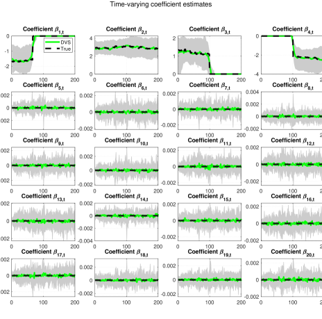
Figure 1: VBDVS coefficient estimates of the first 20 predictors generated from the DGP with $T=200$ and $p=200$. Black dashed lines are the true generated coefficients. Posterior medians (over the 100 Monte Carlo iterations) of VBDVS estimates are shown with green solid lines, and grey areas denote 16^th and 84^th percentiles.

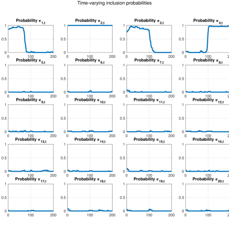
Figure 2: Time-varying posterior inclusion probabilities (expected value of $\gamma_{j,t}$ estimates) of the first 20 predictors generated from the DGP with $T=200$ and $p=200$. These probabilities are means over the 100 Monte Carlo iterations.

Figure 1 shows the coefficient estimates from VBDVS for the case $T=p=200$. This plot compares the posterior median (green solid lines) versus the true generated coefficients (black dashed lines). The 16^th and 84^th percentiles over the 100 Monte Carlo iterations are also shown as a shaded area around the posterior median. Only the first 20 coefficients, out of the possible 200, are plotted. The first row shows the four coefficients that, at least in some periods, are non-zero, followed by 16 coefficients that are exactly zero. It is impossible to plot the remaining 180 coefficients in the DGP that are exactly zero, but their estimates are represented fairly well by the estimates of coefficients $\beta_{5,t}$ - $\beta_{20,t}$ shown in Figure 1. Under the assumption of sparsity in the DGP, the VBDVS algorithm is able to recover the true coefficients with accuracy. Not only the coefficients that are zero in the DGP in all periods are correctly estimated to be zero, but also the three coefficients that are zero only in certain subsamples are estimated precisely. When a coefficient is initially zero and later in the sample becomes important (see coefficient $\beta_{4,t}$), and vice-versa (see coefficients $\beta_{1,t}$ and $\beta_{3,t}$), the dynamic variable selection algorithm is able to identify and jump quickly to the new state. Figure 2 shows that the true reason why estimation is so precise – even in such a demanding case with 200 time-varying coefficients for only 200 observations – is because the estimates of the time-varying posterior inclusion probabilities (PIPs) of each predictor are recovered with precision in the first instance. By identifying correctly which variables should be excluded from the regression model in each period results in shrinking many coefficients to zero and allowing to preserve enough degrees of freedom for estimation of non-zero coefficients.

Table 1 shows the values of the MSD statistics for the three algorithms under the different combinations of $T$ and $p$. Given that the MSD statistics measure deviation from the true coefficient, lower values imply that a certain estimation algorithm has done better recovery of the coefficients generated by the DGP. In all cases VBDVS has the best performance among all competing algorithms. The estimation error of the MCMC algorithm is quite large mainly because the algorithm is unable to shrink all $p-4$ coefficients in the DGP that are exactly zero. The DSS algorithm provides a better fit since it is also an algorithm that does dynamic variable selection and shrinkage. Its performance is slightly inferior to VBDVS, but the results should not be taken as final evidence. While we have done all effort to follow the settings suggested by Ročková and McAlinn (2017), there might be other priors that could improve the performance of this algorithm.

Another important feature of the VBDVS algorithm is its fast computing time. While it is not surprising that our algorithm is faster compared to MCMC, our algorithm can provide substantial savings in high-dimensional settings compared to the DSS that relies on the EM algorithm. Columns 6-8 in Table 1 reveals that VBDVS can be multiple times faster than both DSS and MCMC algorithms.

Table 1: MSD statistics and computing time for Monte Carlo exercise

		MSD statistic				Computing time (secs)
		VBDVS	DSS	MCMC		VBDVS	DSS	MCMC
	$p=50$	0.203	0.419	7.979		1.2	8.3	22.6
$T=100$	$p=100$	0.469	1.014	11.787		7.2	20.1	106.6
	$p=200$	0.536	1.915	14.628		29.9	45.8	402.0
	$p=50$	0.047	0.256	5.825		5.5	19.9	49.9
$T=200$	$p=100$	0.088	0.789	10.583		10.1	40.1	232.2
	$p=200$	0.165	1.780	17.983		38.6	91.9	841.4
	$p=50$	0.019	0.147	4.613		8.3	51.1	125.2
$T=500$	$p=100$	0.043	0.819	9.095		50.9	125.1	555.6
	$p=200$	0.085	1.679	18.398		83.6	220.6	2127.8

Notes: Computing times are based on a Windows 10 laptop running MATLAB 2020a, featuring an Intel i7-8665U processor and 32GB of RAM.

5 Macroeconomic Forecasting with Many Predictors

5.1 A new large dataset for forecasting inflation

Following a large literature on time-varying parameter models in macroeconomics, our primary target is to forecast quarterly US inflation. While there exists mixed empirical evidence about the potential of very large datasets to improve forecasts of inflation, our aim is to demonstrate here that the new dynamic variable selection methodology can successfully extract, period-by-period, predictive information from a large number of predictors. For that reason we build a novel, high-dimensional dataset that brings together predictors from several mainstream aggregate macroeconomic and financial datasets. Our building block is the FRED-QD dataset of McCracken and Ng (2020), which we augment with portfolio data used in Jurado et al. (2015), stock market predictors from Welch and Goyal (2007), survey data from University of Michigan consumer surveys, commodity prices from the World Bank’s Pink Sheet database, and key macroeconomic indicators from the Federal Reserve Economic Data for four economies (Canada, Germany, Japan, UK). All data are quarterly, and span the period 1960Q1-2018Q4. All variables are adjusted from their respective sources for seasonality (where relevant), and we additionally remove extreme outliers.

The dataset has in total 444. Out of these we forecast the series (FRED-QD mnemonics in parentheses): GDP deflator (GDPCTPI), total CPI (CPIAUCSL), core CPI (CPILFESL), and PCE deflator (PCECTPI). When each of these price series, $P_{t}$, is used as the dependent variable to be forecasted $h$-quarters ahead we transform it according to the formula $y_{t+h}=(400/h)\ln\left(P_{t+h}-P_{t}\right)$. We forecast these transformed series one at a time, and the remaining three price series are included in the list of exogenous predictor variables (443 in total). The predictor variables are transformed using standard norms in the literature (see for example McCracken and Ng, 2020): i) levels for variables that are already expressed in rates (e.g. unemployment, interest); ii) first differences of logarithm for variables measuring population (e.g. employment), variables expressed in dollars (e.g. GDP), commodity prices, and some indexes (e.g. Industrial production); and iii) second differences of logarithm for price and consumption indexes, as well as deflator series. The online supplement describes in detail all variables and transformations, and provides links to all sources.

5.2 How the dynamic variable selection algorithm works: An in-sample assessment

Before we set up a comprehensive out-of-sample forecasting exercise, we first assess in-sample estimates from the VBDVS by doing small sensitivity analysis to various prior choices. This exercise is intended to demonstrate that the new algorithm provides reasonable estimates of trends, volatilities and other parameters. Most importantly it serves as a way to clarify that, despite the fact that our prior is heavily parametrized, prior elicitation in the VBDVS algorithm becomes a reasonably straightforward task. As it is impossible to present estimates of the TVP model using all variables in our dataset as predictors, we focus on a small TVP model where GDP deflator regressed on an intercept, two own lags, and the first five principal components from the 443 exogenous predictors (eight predictors in total).

Out of all parameters and hyperparameters defined in our algorithm it is only a handful that are crucial for inference and forecasting, while others can be fixed to reasonable or uninformative values and possibly have little effect on forecasting. Table 2 lists all hyperparameters one need to choose in the VBDVS algorithm, and does an explicit separation into “Important” and “Fixed” hyperparameters. Starting from the latter, $a_{0}$ and $b_{0}$ are the initial scale and rate parameters of the initial condition of the precision parameter in equation (34). Setting $a_{0}=b_{0}=0.01$ implies that the precision has prior mean one and variance 10, which is a reasonable uninformative choice for an inverse variance parameter. Next, we set $\delta=0.8$ for reasons explained in subsection 3.2. Given that $p$ is very large to allow us to obtain meaningful prior information about the regression coefficients $\boldsymbol{\beta}_{t}$ (e.g. using a training sample), we allow their initial condition $\boldsymbol{\beta}_{0}$ to be fairly uninformative by setting $\boldsymbol{m}_{0}=\boldsymbol{0}$ and $\boldsymbol{P}_{0}=4\boldsymbol{I}_{p}$. The parameter $\underline{c}$ in the dynamic variable selection prior has to be small (see discussion in subsection 3.1) and how small it exactly is, affects the way the algorithm selects each of the two Normal components in the spike and slab prior – that is, it affects the choice between a certain $\beta_{j,t}$ being restricted or not. We prefer to fix this parameter to $\underline{c}=0.0001$ and allow only $\tau_{j,t}^{2}$ and its prior to determine the ratio of the prior variances of the two Normal components in the mixture prior.

Table 2: Hyperparameter choices for sensitivity analysis

	Prior 1	Prior 2	Prior 3	Notes
Important hyperparameters
$g_{0}$	$0.01$	$0.01$	$1$	see eq. (24)
$h_{0}$	$0.01$	$0.01$	$12$	see eq. (24)
$c_{j,0}$	$100$	$1$	$100$	see eq. (11)
$d_{j,0}$	$1$	$1$	$1$	see eq. (11)
Fixed hyperparameters
$\underline{c}$	$10^{-4}$	$10^{-4}$	$10^{-4}$	see eq. (22)
$a_{0}$	$0.01$	$0.01$	$0.01$	see eq. (34)
$b_{0}$	$0.01$	$0.01$	$0.01$	see eq. (34)
$\delta$	$0.8$	$0.8$	$0.8$	see eq. (34)
$m_{j,0}$	$0$	$0$	$0$	see eq. (11)
$P_{j,0}$	$4$	$4$	$4$	see eq. (11)

The parameters that are important in our high-dimensional setting are the ones affecting the two prior variances of the time-varying coefficients $\boldsymbol{\beta}_{t}$, namely the hyperparameters of $\tau_{j,t}^{2}$ and $w_{j,t}$. Our first prior choice, denoted as “Prior 1” in Table 2, selects $c_{j,t}=100,d_{j,t}=1$ such that $w_{j,t}$ has a prior mean of 0.01 and prior variance 0.0001. This conservative choice restricts movements $\beta_{j,t}$ to be very persistent and excludes the case of frequent, noisy jumps. Such prior is used widely in empirical macroeconomic applications, see for example the “business as usual” prior motivated in Cogley and Sargent (2005) for the case of a vector autoregression with time-varying parameters. We subsequently set an uninformative prior on $\tau_{j,t}^{2}$ by setting $g_{0}=h_{0}=0.01$. The dashed lines in Figure 3 represent (posterior mean) coefficient estimates from our eight-predictor model: coefficient $\beta_{1,t}$ is the time-varying intercept (trend inflation), coefficients $\beta_{2,t},\beta_{3,t}$ correspond to the first two lagged values of GDP deflator, and coefficients $\beta_{4,t}$ to $\beta_{8,t}$ correspond to the five principal components. As a comparison, we plot posterior mean estimates from the same time-varying parameter regression estimated with MCMC (using identical settings as in the Monte Carlo comparison). The MCMC-based estimates can be broadly thought of as the unrestricted equivalents of the VBDVS algorithm, since they are not based on any form of dynamic variable selection or hierarchical shrinkage. The intercept and first lag coefficients are virtually identical using the two algorithms. However, all remaining coefficients are penalized heavily by the VBDVS algorithm. Variation over time of these coefficients is very moderate and restricted to be close to zero for many time periods.

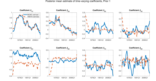
Figure 3: Posterior means of time-varying coefficient estimates from VBDVS (red dashed lines) using Prior 1. Solid lines are posterior means from a TVP model with the same predictors estimated with MCMC.

In order to examine the effect that the prior has on the time evolution of the coefficients, we change the initial condition for $w_{j,t}$ to have hyperparameters $c_{j,0}=d_{j,0}$ and we leave the same uninformative prior for $\tau_{j,t}^{2}$. The posterior mean coefficient estimates in Figure 4 exhibit an interesting pattern. By allowing a looser prior on $w_{t}$ the parameters that are unrestricted (intercept and first lag), do exhibit larger amount of time-variation compared to the MCMC estimates. However, the remaining coefficients that were previously restricted to be close to zero, are now forced more aggressively towards zero in all time periods. This demonstrates the fact that our algorithm imposes the state-space model in equation (28), where the variance of $\beta_{j,t}$ is a function of both $w_{j,t}$ and $v_{j,t}$ (where the latter, is in turn a linear function of $\tau_{j,t}^{2}$). Therefore, allowing for a looser $w_{j,t}$ tends to introduce more noise in the state-space model, and for that reason the dynamic variable selection prior compensates for this increased noise by shrinking more aggressively. While there is this compensation effect and coefficient estimates won’t explode as quickly as the model without the dynamic variable selection prior (recall that $\beta_{j,t}$ evolves as a non-stationary random walk), it is not advisable to use such a lose prior on $w_{j,t}$.

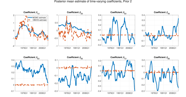
Figure 4: Posterior means of time-varying coefficient estimates from VBDVS (red dashed lines) using Prior 2. Solid lines are posterior means from a TVP model with the same predictors estimated with MCMC.

For that reason, our final prior (called Prior 3 in Table 2) returns to the conservative choice $c_{j,0}=100$ and $d_{j,0}=1$, and sets instead $g_{0}=1$ and $h_{0}=12$. Figure 5 shows the estimates from this prior. Once again the VBDVS estimates of the intercept and first lag coefficients are identical to the estimates from the MCMC algorithm. The remaining coefficients are again heavily penalized but there are also many time periods where these evolve unrestrictedly. As a matter of fact, this prior allows the time-varying coefficients to exhibit distinct and abrupt jumps between periods where they are zero and periods where they are unrestricted. This pattern of time-variation is more in line with the findings of the previous literature that there are pockets of predictability or, put differently, that economic predictors are short-lived (see discussion in the Introduction).

In order to have a visual assessment of the time pattern of dynamic variable selection and shrinkage, panel (a) of Figure 6 plots the posterior inclusion probabilities of each regressor associated with the time-varying coefficient estimates presented in Figure 5. These seem to show the exact periods where each coefficient moves from a state of being restricted to zero to a state where it is not zero. Panel (b) of the same figure shows the posterior mean of the stochastic volatility estimate from VBDVS versus the estimate from MCMC. These two estimates are fairly similar, showing that the specification of time-varying variances in the VBDVS does a good job at capturing known peaks in GDP deflator inflation volatility. Any differences in volatility estimates reflect the fact that the two algorithms assume different specification of $\sigma_{t}^{2}$ and also use different priors in the estimation of $\boldsymbol{\beta}_{t}$.

For all these reason, we build all of our forecasting models in the next subsection based on this last prior.

Figure 5: Posterior means of time-varying coefficient estimates from VBDVS (red dashed lines) using Prior 3. Solid lines are posterior means from a TVP model with the same predictors estimated with MCMC.

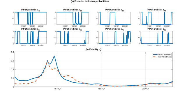
Figure 6: Panel (a) shows time-varying posterior inclusion probabilities (PIPs) from VBDVS algorithm, using Prior 3. Panel (b) shows posterior means of time-varying volatility estimates from VBDVS (red dashed line) versus MCMC (solid blue line).

5.3 Forecasting inflation

We forecast inflation using models of the form

$$y_{t+h}=\alpha_{t}+\phi_{1,t}y_{t}+\phi_{2,t}y_{t-1}+\boldsymbol{x}_{t}\boldsymbol{\beta}_{t}+\varepsilon_{t+h},$$ (45)

where $y_{t+h}$ is $h$-step ahead inflation (see subsection 5.1 for a definition) regressed on an intercept, two own lags and exogenous predictors. We use a variety of forecasting models. Some benchmark models are based on equation (45) but assume constant coefficients (i.e. $\alpha_{t}=\alpha$, $\phi_{1,t}=\phi_{1}$ and so on), while others assume different sets of exogenous predictors. However, what all models have in common is that they always include an intercept and two own lags of inflation. Given that our dataset is much larger than datasets used before for forecasting inflation, in order to avoid confusion by specifying different combinations or subsets of predictors, we only distinguish four simple categories of models: i) models with no predictors (i.e. only intercept and autoregressive terms); ii) models with first five principal components as predictors; iii) models with sixty principal components as predictors; and iv) models with all 443 predictors. Our list of models representing each category is the following

• AR: benchmark AR(2) with intercept, estimated with OLS

• TVPAR: time-varying parameter version of the AR model, with stochastic volatility, estimated with MCMC

• FAC5: Builds on benchmark AR specification by augmenting it with first five principal components estimated with OLS

• BAG/FAC5: Same predictors as FAC5, estimated as constant parameter regression using the Bagging algorithm of Breiman (1996)

• DMA/FAC5: Same predictors as FAC5, estimated as TVP regression using the Dynamic Model Averaging algorithm of Koop and Korobilis (2012)

• VBDVS/FAC5: Same predictors as FAC5, estimated as TVP regression using our Dynamic Variable Selection prior with Variational Bayes

• GPR/FAC5: Same predictors as FAC5, estimated as a Gaussian Process Regression

• SSVS/FAC60: Builds on benchmark AR specification by augmenting it with first 60 principal components, estimated using the SSVS prior with MCMC of George and McCulloch (1993)

• ELN/FAC60: Same predictors as SSVS/FAC60, estimated as a constant parameter regression using the Elastic Net algorithm of Zou and Hastie (2005)

• VBDVS/FAC60: Same predictors as SSVS/FAC60, estimated as a TVP regression using our Dynamic Variable Selection prior with Variational Bayes

• ELN/X: Builds on benchmark AR specification by augmenting it with all 443 predictors, estimated using the Elastic Net algorithm of Zou and Hastie (2005)

• PLS/X: Same predictors as in ELN/X, estimated as a constant parameter Partial Least Squares regression

• VBDVS/X: Same predictors as ELN/X, estimated as a TVP regression using our Dynamic Variable Selection prior with Variational Bayes

The choice of models is based on their simplicity and replicability. In particular, the Gaussian Process Regression, Partial Least Squares, and Elastic Net algorithms are based on built-in functions in MATLAB’s Statistics and Machine Learning Toolbox (MATLAB, 2020), and are fairly easy to set up. Estimation of these models is done using default settings in MATLAB or default choices proposed by their respective creators. Exact details of these algorithms and their default settings is provided in the Online Supplement.

In terms of statistical properties, all these models cover a wide spectrum of forecasting specifications. The AR(2) is a standard benchmark in economic time series forecasting, and typically performs better than a random walk (which is the benchmark for financial data). Its time-varying parameter counterpart, our second model on the list, allows for proxying for similar specifications that have been shown to forecast inflation well, see Stock and Watson (2007) and Bauwens et al. (2015). Extracting the first few principal components (factors) is possibly the most popular way of representing parsimoniously the information in a large dataset, see Stock and Watson (2016). A naive factor model uses least squares estimation on a model that has the first five principal components as exogenous predictors, while a second factor model replaces OLS with the Bagging algorithm of Breiman (1996) that allows to select the “best” factors in a static way. Next the Dynamic Model Averaging (DMA) algorithm described in Koop and Korobilis (2012) as well as our VBDVS algorithm allow to implement dynamic variable selection in a TVP setting using the same first five principal components. The Gaussian Process Regression is a very flexible nonparametric method that allows us to understand whether inflation is better described by time-varying parameters or some more complex form of nonlinearity. Moving on to models with 60 factors, we have to drop many previous specifications for computational reasons. For that reason we use the SSVS algorithm of George and McCulloch (1993), which can be thought of as the static equivalent of our VBDVS algorithm. The Elastic Net of Zou and Hastie (2005) is a popular penalized likelihood estimator for high-dimensional data. Finally, our VBDVS algorithm is also estimated with a larger number of factors to find out whether its dynamic shrinkage properties are useful relative to the naive selection of the first five factors. Finally, we estimate models using all 443 exogenous predictors. The Elastic Net is again on the list, and we also include Partial Least Squares (PLS) regression. PLS is similar to principal component analysis, with the main difference being that factors are extracted with reference to the variable to be predicted. Principal components instead only explain the variability in the exogenous predictors, and it may be the case that they do not carry predictive information for the predicted variable. Finally, our VBDVS algorithm is applied to this full model with all predictors.

In terms of the prior choices used when forecasting with our VBDVS algorithm, these are based on Prior 3 described in the previous subsection, see Table 2. We only adapt how “aggressively” we shrink based on the total number of predictors in each model. For model VBDVS/FAC5 we set $h_{0}=1$, for VBDVS/FAC60 we set $h_{0}=12$ and for VBDVS/X we set $h_{0}=100$.

Table 3: Forecasting results for GDP deflator (GDPCTPI)

		MSFE					ALPL
	$h=1$	$h=2$	$h=4$	$h=8$		$h=1$	$h=2$	$h=4$	$h=8$
Models with no predictors
AR	0.0394	0.0323	0.0308	0.0487		4.8742	4.8949	4.8374	4.6149
TVPAR	1.04	0.96	0.99	0.83		0.30	0.29	0.46	0.31
Models with five factors
FAC5	1.00	1.08	1.53	1.57		0.02	0.04	0.02	0.01
BAG/FAC5	0.96	1.05	1.47	1.48		0.05	0.06	0.04	0.02
DMA/FAC5	0.84	0.79	0.94	0.95		0.26	0.27	0.22	0.18
VBDVS/FAC5	1.30	1.20	0.97	0.83		0.15	0.14	0.28	0.20
GPR/FAC5	1.02	0.95	1.07	1.04		0.06	0.13	0.20	0.32
Models with 60 factors
SSVS/FAC60	0.99	1.03	1.44	1.42		0.01	0.05	0.09	0.13
ELN/FAC60	1.13	1.12	1.24	1.30		0.02	0.07	0.14	0.09
VBDVS/FAC60	1.03	0.81	0.85	0.80		0.25	0.49	0.63	0.92
Models with 443 predictors
ELN/X	0.97	1.00	1.35	1.39		0.06	0.04	0.12	0.05
PLS/X	1.14	1.11	1.42	1.24		-0.11	0.02	-0.24	-0.42
VBDVS/X	0.99	0.84	0.71	0.62		0.32	0.39	0.65	0.78

Notes: All models feature an intercept and two lags of the dependent variable. Model acronyms are as follows:
AR: benchmark AR(2) with intercept estimated with OLS
TVPAR: time-varying parameter version of the AR model, with stochastic volatility, estimated with MCMC
FAC5: Builds on benchmark AR specification by augmenting it with first five principal components estimated with OLS
BAG/FAC5: Same predictors as FAC5, estimated as constant parameter regression using Bagging
DMA/FAC5: Same predictors as FAC5, estimated as TVP regression using Dynamic Model Averaging
VBDVS/FAC5: Same predictors as FAC5, estimated as TVP regression using our Dynamic Variable Selection prior with Variational Bayes
GPR/FAC5: Same predictors as FAC5, estimated as a Gaussian Process Regression
SSVS/FAC60: Builds on benchmark AR specification by augmenting it with first 60 principal components, estimated using an SSVS prior with MCMC
ELN/FAC60: Same predictors as SSVS/FAC60, estimated as a constant parameter regression using the Elastic Net
VBDVS/FAC60: Same predictors as SSVS/FAC60, estimated as a TVP regression using our Dynamic Variable Selection prior with Variational Bayes
ELN/X: Builds on benchmark AR specification by augmenting it with all 443 predictors, estimated using the Elastic Net
PLS/X: Same predictors as in ELN/X, estimated as a constant parameter Partial Least Squares regression
VBDVS/X: Same predictors as ELN/X, estimated as a TVP regression using our Dynamic Variable Selection prior with Variational Bayes
Entries in columns 2-5 of this Table are mean squared forecast errors (MSFEs), and columns 6-9 are average predictive likelihoods in logarithms (logAPLs). The AR model serves as a benchmark and its entries (shown in italics) are the values of MSFEs and logAPLs for each forecast horizon. Entries for each subsequent model are MSFEs and logAPLs relative to the values of the AR benchmark. MSFEs lower than one signify improvement relative to the benchmark and vice-versa for values higher than one. logAPLs that are positive signify improvement relative to the benchmark and vice-versa for negative values. Entries in boldface indicate the best performing model for each forecast statistic and for each forecast horizon.

Table 4: Forecasting results for PCE deflator (PCECTPI)

		MSFE					ALPL
	$h=1$	$h=2$	$h=4$	$h=8$		$h=1$	$h=2$	$h=4$	$h=8$
Models with no predictors
AR	0.1442	0.1301	0.1070	0.0980		4.6028	4.6527	4.5695	4.4313
TVPAR	1.10	1.04	0.81	0.57		0.08	0.24	0.62	0.67
Models with five factors
FAC5	1.10	1.23	1.32	1.40		0.02	0.03	0.05	0.06
BAG/FAC5	1.13	1.27	1.33	1.38		0.04	0.06	0.07	0.05
DMA/FAC5	1.14	1.13	1.02	0.86		-0.07	-0.02	0.05	0.27
VBDVS/FAC5	0.92	0.95	0.75	0.71		-0.09	-0.14	-0.21	0.29
GPR/FAC5	1.08	1.17	1.00	0.96		0.06	0.22	0.31	0.23
Models with 60 factors
SSVS/FAC60	0.98	1.18	1.19	1.37		0.07	0.11	0.17	0.28
ELN/FAC60	0.84	1.04	1.03	0.95		0.16	0.20	0.24	0.32
VBDVS/FAC60	1.11	1.04	0.70	0.51		0.05	0.22	0.54	1.02
Models with 443 predictors
ELN/X	0.73	0.97	1.06	1.00		0.22	0.13	0.12	0.02
PLS/X	0.81	0.91	0.95	0.82		0.12	0.07	0.15	-0.05
VBDVS/X	0.93	0.84	0.62	0.51		0.11	0.27	0.57	0.69

Notes: see notes under Table 3.

Table 5: Forecasting results for CPI (CPIAUCSL)

		MSFE					ALPL
	$h=1$	$h=2$	$h=4$	$h=8$		$h=1$	$h=2$	$h=4$	$h=8$
Models with no predictors
AR	0.1838	0.2247	0.1621	0.1425		4.3741	4.3776	4.3663	4.2359
TVPAR	0.93	0.96	0.73	0.57		0.09	0.42	0.59	0.96
Models with five factors
FAC5	0.95	0.96	1.05	1.03		0.04	0.09	0.03	0.16
BAG/FAC5	0.95	0.97	1.01	0.92		0.06	0.10	0.09	0.16
DMA/FAC5	0.93	0.91	0.87	0.67		-0.02	0.00	0.02	0.35
VBDVS/FAC5	1.07	1.15	0.71	0.75		0.06	0.43	-0.12	0.40
GPR/FAC5	0.93	0.90	0.79	0.82		0.12	0.30	0.29	0.25
Models with 60 factors
SSVS/FAC60	0.89	0.87	0.93	0.87		0.06	0.13	0.14	0.31
ELN/FAC60	1.08	0.81	0.89	0.72		-0.01	0.20	0.22	0.39
VBDVS/FAC60	0.98	0.88	0.67	0.54		0.10	0.45	0.56	1.01
Models with 443 predictors
ELN/X	0.84	0.84	0.92	0.89		0.21	0.27	0.19	0.23
PLS/X	0.95	0.89	0.96	0.89		0.08	0.34	0.21	0.26
VBDVS/X	0.94	0.82	0.64	0.50		0.24	0.33	0.47	0.81

Notes: see notes under Table 3.

Table 6: Forecasting results for core CPI (CPILFESL)

		MSFE					ALPL
	$h=1$	$h=2$	$h=4$	$h=8$		$h=1$	$h=2$	$h=4$	$h=8$
Models with no predictors
AR	0.0221	0.0195	0.0287	0.0549		4.6432	4.6832	4.6294	4.4824
TVPAR	1.00	0.85	0.79	0.48		0.52	0.55	0.58	0.54
Models with five factors
FAC5	1.89	2.37	2.17	1.41		0.02	0.04	0.09	0.15
BAG/FAC5	1.62	2.15	1.90	1.26		0.06	0.08	0.14	0.16
DMA/FAC5	1.17	1.23	0.94	0.60		0.36	0.42	0.48	0.56
VBDVS/FAC5	1.49	1.24	0.90	0.53		0.54	0.39	0.67	0.48
GPR/FAC5	1.66	1.79	1.44	0.99		0.34	0.37	0.68	0.50
Models with 60 factors
SSVS/FAC60	1.73	2.18	2.00	1.05		0.03	0.04	0.13	0.19
ELN/FAC60	1.91	2.09	1.81	0.99		0.05	0.04	0.26	0.32
VBDVS/FAC60	0.91	0.79	0.72	0.47		0.72	0.78	0.93	0.92
Models with 443 predictors
ELN/X	1.79	1.96	1.47	1.21		0.22	0.11	0.37	-0.05
PLS/X	2.53	2.87	2.05	1.27		0.13	0.00	0.14	0.19
VBDVS/X	0.99	0.78	0.60	0.43		0.71	0.78	0.99	1.07

Notes: see notes under Table 3.

We forecast $h=1,2,4$ and $8$ quarters ahead. We use 50% of the sample as our initial estimation period which, for example, for $h=1$ translates to using data for the period 1960Q4-1989Q2 in order to forecast 1989Q3. We then add one new observation to the estimation sample and forecast $h$-step ahead, until the full sample is exhausted. Since all models that have predictors rely on the direct forecasting regression (45), for comparability we produce direct AR(2) forecasts as a special case of this equation with no predictors. We measure forecast accuracy using the mean squared forecast error (MSFE) and the average log-predictive likelihood (ALPL). The first measure is the square of the forecast error (difference between forecast and real value of $y_{t+h}$) averaged over the out-of-sample evaluation period, while the second measure is calculated as the logarithm of the predictive distribution evaluated at the observation $y_{t+h}$ and also averaged over the out-of-sample evaluation period; see Bauwens et al. (2015) for more details on these two metrics.

Tables 3, 4, 5 and 6 present the MSFEs and ALPLs for GDP deflator, PCE deflator, CPI and Core CPI, for all competing models and all considered forecast horizons. To be precise results for the benchmark AR(2) are the values of the MSFE and ALPL statistics, while results for all other models are relative to those for the AR(2). For the MSFE this means calculating the ratio such that a number lower than one means that a certain model performs better than the AR(2). For the ALPL relative quantities are obtained as the spread from the ALPL of the AR(2) (i.e. the logarithm of the ratio) such that positive numbers indicate that a certain model performs better than the AR(2).

The immediate message from these tables is that the VBDVS/X is the model that performs best, especially when looking at point forecast evaluation (MSFEs) for $h=2,4,8$. In terms of density forecasts, VBDVS/X and VBDVS/FAC60 are jointly the best performing specifications. While VBDVS/FAC5 is also doing well in longer horizons, this model is always underperforming the TVPAR, that is, the TVP model that doesn’t consider any predictors.

How can we explain these results? There are various stylized facts we can derive from the information in these tables. Our discussion here focuses on point forecasts (MSFE criterion), due to the fact for that metric the picture is much clearer. First, time variation seems to matter a lot, especially in the long-run. TVPAR, DMA/FAC5, and the three VBDVS specifications can improve dramatically over their constant parameter counterparts, regardless of whether these consider exogenous predictors or not. Are exogenous predictors important for forecasting? The answer depends on the variable to be forecast, the horizon considered, as well as the way each model specification utilizes the predictors. For example, for GDP deflator for $h=8$ the differences in MSFE between VBDVS/X (TVP model with all available predictors) and TVPAR (TVP model with no predictors) is vast, suggesting that not only time-variation is important but also the information in exogenous predictors. However, looking at all constant parameter models with exogenous predictors, whether these predictors are observed or enter each regression via factor methods, all these methods struggle to beat the simple AR(2). This suggests the argument in the Introduction about pockets of predictability. For that reason, DMA (which is the best performing model for $h=1$ and $h=2$) and the three VBDVS specifications perform very well, with VBDVS/X providing the most dramatic improvements for $h=8$ when at the same time ELN/X and PLS/X perform 24% and 39% worse than the benchmark AR(2).

For the next two inflation variables (PCE deflator and total CPI) a large number of predictors does seem to be important in the short-run, but in the long-run it looks like the largest contribution in forecasting accuracy is due to time-variation in parameters. For example, for PCE deflator and total CPI, for horizons $h=1,2$, ELN/X seems to be performing much better than the AR and the TVPAR specifications. However, for $h=4,8$ the TVPAR overtakes substantially both the AR and ELN/X specifications. While the VBDVS/X is still the best performing model for $h=4,8$, its differences to the TVPAR are statistically much smaller compared to the differences of these two models when forecasting GDP deflator. In any case, whether predictors are important or not, the VBDVS algorithm seems to be doing a very good job in shrinking irrelevant coefficients and making sure that there is not overfitting – if there was, the VBDVS/X forecasts would be inferior to those from the TVPAR.

Finally, for core CPI all methods struggle to beat the simple AR for very short-run forecasts. The VBDVS/FAC60 and VBDVS/X models do so marginally, while many others perform as much as 150% worse than the benchmark. For longer horizons all constant parameter models continue to underperform, however, the TVP models seem to provide the most dramatic improvements, with the VBDVS/X improving almost 60% over the benchmark. Combined with the observation that the differences between the three VBDVS specifications and the TVPAR are minimal, it looks like that exogenous predictors are not relevant for core CPI. Since core CPI is based on the total CPI by removing its most volatiles components (food and energy), it might be the case that this variable is basically a random walk and even a simple time-varying intercept model (that is, a local level model as in Stock and Watson, 2007) would forecast this variable well.

It is harder to extract stylized facts for inflation forecasting based on ALPLs. This is because this metric is based on all the features of the predictive density, that is, all its moments and not just the mean. Given that predictive densities can differ a lot between specifications (e.g. they can multimodal in time-varying parameter models), it is not possible to attribute differences in ALPLs to specific modeling assumptions. However, a clear pattern that emerges is that predictors do help to improve predictive density forecasting relative to the simple AR benchmark, but the largest gains overall are achieved by time-varying parameter models. In all these comparisons the VBDVS/X is the clear winner showing that, even though this is a heavily parametrized model and could easily produce erroneous forecasts, our algorithm ensures sufficient penalization and impressive forecasting gains.

Appendix A Settings used in competing models

While all technical details regarding our methodology are provided in detail in the paper, we have skipped details for the numerous competing algorithms used in the Monte Carlo and empirical exercises.

• DSS algorithm, Ročková and McAlinn (2017): We followed the authors and tried the various settings they suggest in their Section 7: Synthetic high-dimensional data. For our DGP the best performance was achieved with $\phi_{0}=0$, $\phi_{1}=0.98$, $\lambda_{1}=10*(1-\phi_{1}.^{2})$, $\lambda_{0}=0.9$ and $\Theta=0.92$ (note that for $p=50$ the authors suggest $\Theta=0.98$, but we found that a lower value does better as $p$ gets larger, while it doesn’t deteriorate performance for $p=50$).

• MCMC algorithm, Chan and Jeliazkov (2009): This is the standard time-varying parameter regression model used in economics, see for example Cogley and Sargent (2005). It consists of equations (9) and (10), where the measurement error variance follows a geometric random walk. As with VBDVS, the crucial setting that affects the amount of time-variation in regression coefficients is the prior on the state variances, which is of the form $w_{j}^{-1}\sim Gamma(v_{1},v_{2})$. We set the conservative choice $v_{1}=3$ and $v_{2}=20$, which implies that $w_{j}$ has prior mean around $0.016$. In order to estimate this model efficiently, we use the Gibbs sampler algorithm of Chan and Jeliazkov (2009).

• Dynamic Model Averaging, Koop and Korobilis (2012): We use standard settings described in Koop and Korobilis (2012) with $\alpha=0.99$, $\lambda=0.99$ and $\kappa=0.96$.

• Bagging, Breiman (1996): With the bagging algorithm we first resample our data $B$ times with replacement blocks of size $m$. For each pseudo-generated dataset we estimate with ordinary least squares using the Newey and West estimator of the covariance with lag truncation parameter $int\left\{T^{1/4}\right\}$. We select the optimal model using only those predictors that have t-statistics larger than a threshold $c^{\ast}$ in absolute value. We forecast with the optimal model, and the bagging forecast is obtained as the average of all forecasts over the $B$ Bootstrap replications. We set $B=1000$, $m=1$ and $c^{\ast}=2.807$.

• Elastic Net, Zou and Hastie (2005): We use the MATLAB function “lasso” that is available in the Statistics and Machine Learning Toolbox. We use 10-fold cross validation for selecting the optimal $\lambda$ parameter, and we fix $\alpha=0.75$.

• Gaussian Process Regression: Gaussian Process Regression (GPR) is a very powerful machine learning method that allows flexible nonparametric estimation targeted towards prediction. We use the MATLAB function “fitrgp” that is available in the Statistics and Machine Learning Toolbox. This is estimated using the following settings:
  fitrgp(X,y,’Basis’,’linear’,’Optimizer’,’QuasiNewton’,’verbose’,1, ’FitMethod’,’exact’,’PredictMethod’,’exact’)

• Partial Least Squares: Partial Least Squares (PLS) is a method that originated in chemometrics. It allows to estimate factors that are extracted with reference to the variable to be predicted (target variable). Principal components instead maximize only the variance explained by the large dataset, and may not be optimal for prediction of the target variable. While more elegant methods have been proposed recently, such as the three-pass regression filter, the PLS is undeniably a good benchmark for assessing whether we can improve on the information content of simple principal component estimates. We use again the MATLAB function “plsregress” available in the Statistics and Machine Learning Toolbox, and we extract five factors from our dataset.

Appendix B Data Appendix

The following high-dimensional dataset combines several popular datasets used in macroeconomics and finance. The core part builds on the FRED-QD dataset compiled in McCracken and Ng (2020), and the financial (portfolio) data used in Jurado et al. (2015) to extract a popular uncertainty index that are originally provided by Kenneth French (https://mba.tuck.dartmouth.edu/pages/faculty/ken.french/data_library.html). These are augmented with additional consumer survey indicators from University of Michigan (https://data.sca.isr.umich.edu/); predictors of stock returns used in Welch and Goyal (2007) provided by Amit Goyal (http://www.hec.unil.ch/agoyal/); Commodity prices from the World Bank’s Pink Sheet database (https://www.worldbank.org/en/research/commodity-markets); and key macroeconomic indicators for key economies, obtained from Federal Reserve Economic Data (FRED) of St Louis Federal Reserve Bank (https://fred.stlouisfed.org/).

LABEL:datatable presents the 444 variables used in the empirical exercise. These are measured quarterly and cover the period 1960Q1-2018Q4. Where a variable is measured originally in higher frequency (e.g. monthly) quarterly values are obtained by taking the average over the quarter. Column $F$ in LABEL:datatable denotes whether the variable is used or not (1 or 0, respectively) to extract factors (principal components). The idea is that where some variables are aggregates of disaggregated series in the dataset, we only use the disaggregated series to extract factors. Column $F$ denotes the code used in order to transform each variable to be approximately stationary. The transformation codes are the following 1: level (no transformation); 2: first difference; 3: second difference; 4: natural logarithm; 5: first difference of natural logarithm; 6: second difference of natural logarithm; 7: first difference of percent change. The mnemonics used are those provided by the respective resources. For the Welch and Goyal (2007) data in particular, the mnemonics are those provided in the data appendix of that paper. In the $Source$ column of LABEL:datatable, this paper is abbreviated as GW2008.

Table A1: Quarterly large dataset

No	Mnemonic	F	T	Long description	Source
1	GDPC1	0	5	Real Gross Domestic Product	FRED-QD
2	PCECC96	0	5	Consumption Real Personal Consumption Expenditures	FRED-QD
3	PCDGx	1	5	Real personal consumption expenditures: Durable goods	FRED-QD
4	PCESVx	1	5	Real Personal Consumption Expenditures: Services	FRED-QD
5	PCNDx	1	5	Real Personal Consumption Expenditures: Nondurable Goods	FRED-QD
6	GPDIC1	0	5	Real Gross Private Domestic Investment	FRED-QD
7	FPIx	0	5	Real private fixed investment	FRED-QD
8	Y033RC1Q027SBEAx	1	5	Real Gross Private Domestic Fixed Investment: Nonresidential: Equipment	FRED-QD
9	PNFIx	1	5	Real private fixed investment: Nonresidential	FRED-QD
10	PRFIx	1	5	Real private fixed investment: Residential	FRED-QD
11	A014RE1Q156NBEA	1	1	Gross private domestic investment: Change in private inventories	FRED-QD
12	GCEC1	0	5	Real Government Consumption Expenditures & Gross Investment	FRED-QD
13	A823RL1Q225SBEA	1	1	Real Government Consumption Expenditures and Gross Investment: Federal	FRED-QD
14	FGRECPTx	1	5	Real Federal Government Current Receipts	FRED-QD
15	SLCEx	1	5	Real government state and local consumption expenditures	FRED-QD
16	EXPGSC1	1	5	Real Exports of Goods & Services	FRED-QD
17	IMPGSC1	1	5	Real Imports of Goods & Services	FRED-QD
18	DPIC96	0	5	Real Disposable Personal Income	FRED-QD
19	OUTNFB	0	5	Real Disposable Personal Income	FRED-QD
20	OUTBS	0	5	Business Sector: Real Output	FRED-QD
21	INDPRO	0	5	Industrial Production Index	FRED-QD
22	IPFINAL	0	5	Industrial Production: Final Products	FRED-QD
23	IPCONGD	0	5	Industrial Production: Consumer Goods	FRED-QD
24	IPMAT	0	5	Industrial Production: Materials	FRED-QD
25	IPDMAT	1	5	Industrial Production: Durable Materials	FRED-QD
26	IPNMAT	1	5	Industrial Production: Nondurable Materials	FRED-QD
27	IPDCONGD	1	5	Industrial Production: Durable Consumer Goods	FRED-QD
28	IPB51110SQ	1	5	Industrial Production: Durable Goods: Automotive products	FRED-QD
29	IPNCONGD	1	5	Industrial Production: Durable Goods: Automotive products	FRED-QD
30	IPBUSEQ	1	5	Industrial Production: Business Equipment	FRED-QD
31	IPB51220SQ	1	5	Industrial Production: Consumer energy products	FRED-QD
32	CUMFNS	1	1	Capacity Utilization: Manufacturing (SIC)	FRED-QD
33	PAYEMS	0	5	All Employees: Total nonfarm	FRED-QD
34	USPRIV	0	5	All Employees: Total Private Industries	FRED-QD
35	MANEMP	0	5	All Employees: Manufacturing	FRED-QD
36	SRVPRD	0	5	All Employees: Service-Providing Industries	FRED-QD
37	USGOOD	0	5	All Employees: Goods-Producing Industries	FRED-QD
38	DMANEMP	1	5	All Employees: Durable goods	FRED-QD
39	NDMANEMP	0	5	All Employees: Nondurable goods	FRED-QD
40	USCONS	1	5	All Employees: Construction	FRED-QD
41	USEHS	1	5	All Employees: Education & Health Services	FRED-QD
42	USFIRE	1	5	All Employees: Education & Health Services	FRED-QD
43	USINFO	1	5	All Employees: Information Services	FRED-QD
44	USPBS	1	5	All Employees: Professional & Business Services	FRED-QD
45	USLAH	1	5	All Employees: Leisure & Hospitality	FRED-QD
46	USSERV	1	5	All Employees: Other Services	FRED-QD
47	USMINE	1	5	All Employees: Mining and logging	FRED-QD
48	USTPU	1	5	All Employees: Trade, Transportation & Utilities	FRED-QD
49	USGOVT	0	5	All Employees: Government	FRED-QD
50	USTRADE	1	5	All Employees: Retail Trade	FRED-QD
51	USWTRADE	1	5	All Employees: Wholesale Trade	FRED-QD
52	CES9091000001	1	5	All Employees: Government: Federal	FRED-QD
53	CES9092000001	1	5	All Employees: Government: State Government	FRED-QD
54	CES9093000001	1	5	All Employees: Government: Local Government	FRED-QD
55	CE16OV	0	5	Civilian Employment	FRED-QD
56	CIVPART	0	2	Civilian Labor Force Participation Rate	FRED-QD
57	UNRATE	0	2	Civilian Unemployment Rate	FRED-QD
58	UNRATESTx	0	2	Unemployment Rate less than 27 weeks	FRED-QD
59	UNRATELTx	0	2	Unemployment Rate for more than 27 weeks	FRED-QD
60	LNS14000012	1	2	Unemployment Rate - 16 to 19 years	FRED-QD
61	LNS14000025	1	2	Unemployment Rate - 20 years and over, Men	FRED-QD
62	LNS14000026	1	2	Unemployment Rate - 20 years and over, Women	FRED-QD
63	UEMPLT5	1	5	Number of Civilians Unemployed - Less Than 5 Weeks	FRED-QD
64	UEMP5TO14	1	5	Number of Civilians Unemployed for 5 to 14 Weeks	FRED-QD
65	UEMP15T26	1	5	Number of Civilians Unemployed for 15 to 26 Weeks	FRED-QD
66	UEMP27OV	1	5	Number of Civilians Unemployed for 27 Weeks and Over	FRED-QD
67	LNS12032194	1	5	Employment Level - Part-Time for Economic Reasons, All Industries	FRED-QD
68	HOABS	0	5	Business Sector: Hours of All Persons	FRED-QD
69	HOANBS	0	5	Nonfarm Business Sector: Hours of All Persons	FRED-QD
70	AWHMAN	1	1	Average Weekly Hours of Production and Nonsupervisory Employees: Manufacturing	FRED-QD
71	AWOTMAN	1	2	Average Weekly Hours Of Production And Nonsupervisory Employees: Total private	FRED-QD
72	HWIx	0	1	Help-Wanted Index	FRED-QD
73	HOUST	0	5	Housing Starts: Total: New Privately Owned Housing Units Started	FRED-QD
74	HOUST5F	0	5	Housing Starts: Total: New Privately Owned Housing Units Started	FRED-QD
75	PERMIT	1	5	New Private Housing Units Authorized by Building Permits	FRED-QD
76	HOUSTMW	1	5	Housing Starts in Midwest Census Region	FRED-QD
77	HOUSTNE	1	5	Housing Starts in Northeast Census Region	FRED-QD
78	HOUSTS	1	5	Housing Starts in South Census Region	FRED-QD
79	HOUSTW	1	5	Housing Starts in West Census Region	FRED-QD
80	CMRMTSPLx	0	5	Real Manufacturing and Trade Industries Sales	FRED-QD
81	RSAFSx	1	5	Real Retail and Food Services Sales	FRED-QD
82	AMDMNOx	1	5	Real Manufacturers’ New Orders: Durable Goods	FRED-QD
83	AMDMUOx	1	5	Real Manufacturers’ Unfilled Orders for Durable Goods	FRED-QD
84	PCECTPI	0	6	Personal Consumption Expenditures: Chain-type Price Index	FRED-QD
85	PCEPILFE	0	6	Personal Consumption Expenditures Excluding Food and Energy	FRED-QD
86	GDPCTPI	0	6	Gross Domestic Product: Chain-type Price Index	FRED-QD
87	GPDICTPI	1	6	Gross Private Domestic Investment: Chain-type Price Index	FRED-QD
88	IPDBS	1	6	Business Sector: Implicit Price Deflator	FRED-QD
89	DGDSRG3Q086SBEA	0	6	Goods Personal consumption expenditures: Goods	FRED-QD
90	DDURRG3Q086SBEA	0	6	Personal consumption expenditures: Durable goods	FRED-QD
91	DSERRG3Q086SBEA	0	6	Personal consumption expenditures: Services	FRED-QD
92	DNDGRG3Q086SBEA	0	6	Personal consumption expenditures: Nondurable goods	FRED-QD
93	DHCERG3Q086SBEA	0	6	Personal consumption expenditures: Nondurable goods	FRED-QD
94	DMOTRG3Q086SBEA	1	6	Personal consumption expenditures: Durable goods: Motor vehicles and parts	FRED-QD
95	DFDHRG3Q086SBEA	1	6	Personal consumption expenditures: Durable goods: Furnishings and durable equipment	FRED-QD
96	DREQRG3Q086SBEA	1	6	Personal consumption expenditures: Durable goods: Recreational goods and vehicles	FRED-QD
97	DODGRG3Q086SBEA	1	6	Personal consumption expenditures: Durable goods: Other durable goods	FRED-QD
98	DFXARG3Q086SBEA	1	6	Personal consumption expenditures: Nondurable goods: Food and beverages	FRED-QD
99	DCLORG3Q086SBEA	1	6	Personal consumption expenditures: Nondurable goods: Clothing and footwear	FRED-QD
100	DGOERG3Q086SBEA	1	6	Personal consumption expenditures: Nondurable goods: Gasoline and other energy goods	FRED-QD
101	DONGRG3Q086SBEA	1	6	Personal consumption expenditures: Nondurable goods: Other nondurable goods	FRED-QD
102	DHUTRG3Q086SBEA	1	6	Personal consumption expenditures: Services: Housing and utilities	FRED-QD
103	DHLCRG3Q086SBEA	1	6	Personal consumption expenditures: Services: Health care	FRED-QD
104	DTRSRG3Q086SBEA	1	6	Personal consumption expenditures: Transportation services	FRED-QD
105	DRCARG3Q086SBEA	1	6	Personal consumption expenditures: Recreation services	FRED-QD
106	DFSARG3Q086SBEA	1	6	Personal consumption expenditures: Services: Food services and accommodations	FRED-QD
107	DIFSRG3Q086SBEA	1	6	Personal consumption expenditures: Financial services and insurance	FRED-QD
108	DOTSRG3Q086SBEA	1	6	Personal consumption expenditures: Other services	FRED-QD
109	CPIAUCSL	0	6	Consumer Price Index for All Urban Consumers: All Items	FRED-QD
110	CPILFESL	0	6	Consumer Price Index for All Urban Consumers: All Items Less Food & Energy	FRED-QD
111	WPSFD49207	0	6	Producer Price Index by Commodity for Final Demand: Finished Goods	FRED-QD
112	PPIACO	0	6	Producer Price Index for All Commodities	FRED-QD
113	WPSFD49502	1	6	Producer Price Index by Commodity for Finished Consumer Goods	FRED-QD
114	WPSFD4111	1	6	Producer Price Index by Commodity for Finished Consumer Foods	FRED-QD
115	PPIIDC	1	6	Producer Price Index by Commodity Industrial Commodities	FRED-QD
116	WPSID61	1	6	Producer Price Index by Commodity Intermediate Materials: Supplies & Components	FRED-QD
117	WPU0561	1	5	Producer Price Index by Commodity for Fuels and Related Products and Power: Crude Petroleum	FRED-QD
118	OILPRICEx	0	5	Real Crude Oil Prices: West Texas Intermediate (WTI) - Cushing, Oklahoma	FRED-QD
119	CES2000000008x	0	5	Real Average Hourly Earnings of Production and Nonsupervisory Employees: Construction	FRED-QD
120	CES3000000008x	0	5	Real Average Hourly Earnings of Production and Nonsupervisory Employees: Manufacturing	FRED-QD
121	COMPRNFB	1	5	Manufacturing Sector: Real Compensation Per Hour	FRED-QD
122	RCPHBS	1	5	Business Sector: Real Compensation Per Hour	FRED-QD
123	OPHNFB	1	5	Nonfarm Business Sector: Real Output Per Hour of All Persons	FRED-QD
124	OPHPBS	0	5	Business Sector: Real Output Per Hour of All Persons	FRED-QD
125	ULCBS	0	5	Business Sector: Unit Labor Cost	FRED-QD
126	ULCNFB	1	5	Nonfarm Business Sector: Unit Labor Cost	FRED-QD
127	UNLPNBS	1	5	Nonfarm Business Sector: Unit Nonlabor Payments	FRED-QD
128	FEDFUNDS	1	2	Effective Federal Funds Rate	FRED-QD
129	TB3MS	1	2	3-Month Treasury Bill: Secondary Market Rate	FRED-QD
130	TB6MS	0	2	6-Month Treasury Bill: Secondary Market Rate	FRED-QD
131	GS1	0	2	1-Year Treasury Constant Maturity Rate	FRED-QD
132	GS10	0	2	10-Year Treasury Constant Maturity Rate	FRED-QD
133	AAA	0	2	Moody’s Seasoned Aaa Corporate Bond Yield	FRED-QD
134	BAA	0	2	Moody’s Seasoned Baa Corporate Bond Yield	FRED-QD
135	BAA10YM	1	1	Moody’s Seasoned Baa Corporate Bond Yield Relative to Yield on 10-Year Treasury Constant Maturity	FRED-QD
136	TB6M3Mx	1	1	6-Month Treasury Bill Minus 3-Month Treasury Bill, secondary market	FRED-QD
137	GS1TB3Mx	1	1	1-Year Treasury Constant Maturity Minus 3-Month Treasury Bill, secondary market	FRED-QD
138	GS10TB3Mx	1	1	10-Year Treasury Constant Maturity Minus 3-Month Treasury Bill, secondary market	FRED-QD
139	CPF3MTB3Mx	1	1	3-Month Commercial Paper Minus 3-Month Treasury Bill, secondary market	FRED-QD
140	AMBSLREAL	1	5	St. Louis Adjusted Monetary Base	FRED-QD
141	M1REAL	1	5	Real M1 Money Stock	FRED-QD
142	M2REAL	1	5	Real M2 Money Stock	FRED-QD
143	MZMREAL	1	5	Real MZM Money Stock	FRED-QD
144	BUSLOANSx	1	5	Real Commercial and Industrial Loans, All Commercial Banks	FRED-QD
145	CONSUMERx	1	5	Consumer Loans at All Commercial Banks	FRED-QD
146	NONREVSLx	1	5	Total Real Nonrevolving Credit Owned and Securitized, Outstanding	FRED-QD
147	REALLNx	1	5	Real Real-Estate Loans, All Commercial Banks	FRED-QD
148	TOTALSLx	1	5	Total Consumer Credit Outstanding	FRED-QD
149	TABSHNOx	1	5	Real Total Assets of Households and Nonprofit Organizations	FRED-QD
150	TLBSHNOx	1	5	Real Total Liabilities of Households and Nonprofit Organizations	FRED-QD
151	LIABPIx	0	5	Liabilities of Households and Nonprofit Organizations Relative to Personal Disposable Income	FRED-QD
152	TNWBSHNOx	1	5	Real Net Worth of Households and Nonprofit Organizations	FRED-QD
153	NWPIx	0	1	Net Worth of Households and Nonprofit Organizations Relative to Disposable Personal Income	FRED-QD
154	TARESAx	1	5	Real Assets of Households and Nonprofit Organizations excluding Real Estate Assets	FRED-QD
155	HNOREMQ027Sx	1	5	Real Real-Estate Assets of Households and Nonprofit Organizations	FRED-QD
156	TFAABSHNOx	1	5	Real Total Financial Assets of Households and Nonprofit Organizations	FRED-QD
157	TWEXMMTH	1	5	Trade Weighted U.S. Dollar Index: Major Currencies, Goods	FRED-QD
158	EXSZUSx	1	5	Switzerland / U.S. Foreign Exchange Rate	FRED-QD
159	EXJPUSx	1	5	Japan / U.S. Foreign Exchange Rate	FRED-QD
160	EXUSUKx	1	5	U.S. / U.K. Foreign Exchange Rate	FRED-QD
161	EXCAUSx	1	5	Canada / U.S. Foreign Exchange Rate	FRED-QD
162	UMCSENTx	0	1	University of Michigan: Consumer Sentiment	FRED-QD
163	PAGO	1	1	Current Financial Situation Compared with a Year Ago	UofMich
164	PEXP	1	1	Expected Change in Financial Situation in a Year	UofMich
165	NEWS	1	1	News Heard of Recent Changes in Business Conditions	UofMich
166	BAGO	1	1	Current Business Conditions Compared with a Year Ago	UofMich
167	BEXP	1	1	Expected Change in Business Conditions in a Year	UofMich
168	BUS12	1	1	Business Conditions Expected During the Next Year	UofMich
169	BUS5	1	1	Business Conditions Expected During the Next 5 Years	UofMich
170	INFEXP	1	1	Expected Change in Prices During the Next Year	UofMich
171	DUR	1	1	Buying Conditions for Large Household Durables	UofMich
172	VEH	1	1	Buying Conditions for Vehicles	UofMich
173	HOM	1	1	Buying Conditions for Houses	UofMich
174	USASACRQISMEI	1	1	Passenger Car Registrations in United States	FRED-QD
175	USALOLITONOSTSAM	1	1	Leading indicators: CLI: Normalised for the United States	FRED-QD
176	BSCICP03USM665S	1	1	Composite Indicators: OECD Indicator for the United States	FRED-QD
177	B020RE1Q156NBEA	0	2	Shares of gross domestic product: Exports of goods and services	FRED-QD
178	B021RE1Q156NBEA	0	2	Shares of gross domestic product: Imports of goods and services	FRED-QD
179	IPMANSICS	0	5	Industrial Production: Manufacturing (SIC)	FRED-QD
180	IPB51222S	0	5	Industrial Production: Residential Utilities	FRED-QD
181	IPFUELS	0	5	Industrial Production: Fuels	FRED-QD
182	UEMPMEAN	1	2	Duration of Unemployment	FRED-QD
183	CES0600000007	1	2	Average Weekly Hours of Production and Nonsupervisory Employees: Goods-Producing	FRED-QD
184	TOTRESNS	0	6	Total Reserves of Depository Institutions	FRED-QD
185	NONBORRES	0	7	Reserves of Depository Institutions, Nonborrowed	FRED-QD
186	GS5	0	2	5-Year Treasury Constant Maturity Rate	FRED-QD
187	TB3SMFFM	1	1	3-Month Treasury Constant Maturity Minus Federal Funds Rate	FRED-QD
188	T5YFFM	1	1	5-Year Treasury Constant Maturity Minus Federal Funds Rate	FRED-QD
189	AAAFFM	1	1	Moody’s Seasoned Aaa Corporate Bond Minus Federal Funds Rate	FRED-QD
190	WPSID62	1	6	Producer Price Index: Crude Materials for Further Processing	FRED-QD
191	PPICMM	0	6	Producer Price Index: Commodities: Metals and metal products: Primary nonferrous metals	FRED-QD
192	CPIAPPSL	0	6	Producer Price Index: Commodities: Metals and metal products: Primary nonferrous metals	FRED-QD
193	CPITRNSL	1	6	Consumer Price Index for All Urban Consumers: Transportation	FRED-QD
194	CPIMEDSL	1	6	Consumer Price Index for All Urban Consumers: Medical Care	FRED-QD
195	CUSR0000SAC	1	6	Consumer Price Index for All Urban Consumers: Commodities	FRED-QD
196	CUSR0000SAD	1	6	Consumer Price Index for All Urban Consumers: Durables	FRED-QD
197	CUSR0000SAS	1	6	Consumer Price Index for All Urban Consumers: Services	FRED-QD
198	CPIULFSL	0	6	Consumer Price Index for All Urban Consumers: All Items Less Food	FRED-QD
199	CUSR0000SA0L2	0	6	Consumer Price Index for All Urban Consumers: All items less shelter	FRED-QD
200	CUSR0000SA0L5	0	6	Consumer Price Index for All Urban Consumers: All items less medical care	FRED-QD
201	CES0600000008	0	6	Average Hourly Earnings of Production and Nonsupervisory Employees: Goods-Producing	FRED-QD
202	DTCOLNVHFNM	0	6	Consumer Motor Vehicle Loans Outstanding Owned by Finance Companies	FRED-QD
203	DTCTHFNM	0	6	Total Consumer Loans and Leases Outstanding Owned and Securitized by Finance Companies	FRED-QD
204	INVEST	1	6	Securities in Bank Credit at All Commercial Banks	FRED-QD
205	HWIURATIOx	1	2	Ratio of Help Wanted/No. Unemployed	FRED-QD
206	CLAIMSx	1	5	Initial Claims	FRED-QD
207	BUSINVx	1	5	Total Business Inventories	FRED-QD
208	ISRATIOx	1	2	Total Business: Inventories to Sales Ratio	FRED-QD
209	CONSPIx	0	2	Nonrevolving consumer credit to Personal Income	FRED-QD
210	CP3M	0	2	3-Month AA Financial Commercial Paper Rate	FRED-QD
211	COMPAPFF	0	1	3-Month Commercial Paper Minus Federal Funds Rate	FRED-QD
212	PERMITNE	0	5	New Private Housing Units Authorized by Building Permits in the Northeast Census Region	FRED-QD
213	PERMITMW	0	5	New Private Housing Units Authorized by Building Permits in the Midwest Census Region	FRED-QD
214	PERMITS	0	5	New Private Housing Units Authorized by Building Permits in the South Census Region	FRED-QD
215	PERMITW	0	5	New Private Housing Units Authorized by Building Permits in the West Census Region	FRED-QD
216	NIKKEI225	0	5	Nikkei Stock Average	FRED-QD
217	TLBSNNCBx	0	5	Real Nonfinancial Corporate Business Sector Liabilities	FRED-QD
218	TLBSNNCBBDIx	0	1	Nonfinancial Corporate Business Sector Liabilities to Disposable Business Income	FRED-QD
219	TTAABSNNCBx	0	5	Real Nonfinancial Corporate Business Sector Assets	FRED-QD
220	TNWMVBSNNCBx	0	5	Real Nonfinancial Corporate Business Sector Net Worth	FRED-QD
221	TNWMVBSNNCBBDIx	0	2	Nonfinancial Corporate Business Sector Net Worth to Disposable Business Income	FRED-QD
222	TLBSNNBx	0	5	Real Nonfinancial Noncorporate Business Sector Liabilities	FRED-QD
223	TLBSNNBBDIx	0	1	Nonfinancial Noncorporate Business Sector Liabilities to Disposable Business Income	FRED-QD
224	TABSNNBx	0	5	Real Nonfinancial Noncorporate Business Sector Assets	FRED-QD
225	TNWBSNNBx	0	5	Real Nonfinancial Noncorporate Business Sector Net Worth	FRED-QD
226	TNWBSNNBBDIx	0	2	Nonfinancial Noncorporate Business Sector Net Worth to Disposable Business Income	FRED-QD
227	CNCFx	0	5	Real Disposable Business Income, Billions of 2009 Dollars	FRED-QD
228	S&P 500	1	5	S&P’s Common Stock Price Index: Composite	FRED-QD
229	S&P: indust	0	5	S&P’s Common Stock Price Index: Industrials	FRED-QD
230	S&P div yield	0	2	S&P’s Composite Common Stock: Dividend Yield	FRED-QD
231	S&P PE ratio	0	5	S&P’s Composite Common Stock: Price-Earnings Ratio	FRED-QD
232	d/p	1	2	Dividend Price Ratio	GW2008
233	d/y	1	2	Dividend Yield	GW2008
234	e/p	1	2	Earnings Price Ratio	GW2008
235	d/e	1	2	Dividend Payout Ratio	GW2008
236	b/m	1	2	Book-to-Market Ratio	GW2008
237	svar	1	1	Stock Market Variance	GW2008
238	ntis	1	1	Net Equity Expansion	GW2008
239	lty	1	1	Long Term Yield	GW2008
240	dfy	1	1	Default Yield Spread	GW2008
241	dfr	1	1	Default Return Spread	GW2008
242	Mkt-RF	1	1	Market Excess Return (based on NYSE)	K. French
243	SMB	1	1	Small Minus Big, Sorted on Size	K. French
244	HML	1	1	High Minus Low, Sorted on Book-to-Market	K. French
245	Agric	1	1	Agric Industry Portfolio	K. French
246	Food	1	1	Food Industry Portfolio	K. French
247	Beer	1	1	Beer Industry Portfolio	K. French
248	Smoke	1	1	Smoke Industry Portfolio	K. French
249	Toys	1	1	Toys Industry Portfolio	K. French
250	Fun	1	1	Fun Industry Portfolio	K. French
251	Books	1	1	Books Industry Portfolio	K. French
252	Hshld	1	1	Hshld Industry Portfolio	K. French
253	Clths	1	1	Clths Industry Portfolio	K. French
254	MedEq	1	1	MedEq Industry Portfolio	K. French
255	Drugs	1	1	Drugs Industry Portfolio	K. French
256	Chems	1	1	Chems Industry Portfolio	K. French
257	Rubbr	1	1	Rubbr Industry Portfolio	K. French
258	Txtls	1	1	Txtls Industry Portfolio	K. French
259	BldMt	1	1	BldMt Industry Portfolio	K. French
260	Cnstr	1	1	Cnstr Industry Portfolio	K. French
261	Steel	1	1	Steel Industry Portfolio	K. French
262	Mach	1	1	Mach Industry Portfolio	K. French
263	ElcEq	1	1	ElcEq Industry Portfolio	K. French
264	Autos	1	1	Autos Industry Portfolio	K. French
265	Aero	1	1	Aero Industry Portfolio	K. French
266	Ships	1	1	Ships Industry Portfolio	K. French
267	Mines	1	1	Mines Industry Portfolio	K. French
268	Coal	1	1	Coal Industry Portfolio	K. French
269	Oil	1	1	Oil Industry Portfolio	K. French
270	Util	1	1	Util Industry Portfolio	K. French
271	Telcm	1	1	Telcm Industry Portfolio	K. French
272	PerSv	1	1	PerSv Industry Portfolio	K. French
273	BusSv	1	1	BusSv Industry Portfolio	K. French
274	Hardw	1	1	Hardw Industry Portfolio	K. French
275	Chips	1	1	Chips Industry Portfolio	K. French
276	LabEq	1	1	LabEq Industry Portfolio	K. French
277	Paper	1	1	Paper Industry Portfolio	K. French
278	Boxes	1	1	Boxes Industry Portfolio	K. French
279	Trans	1	1	Trans Industry Portfolio	K. French
280	Whlsl	1	1	Whlsl Industry Portfolio	K. French
281	Rtail	1	1	Rtail Industry Portfolio	K. French
282	Meals	1	1	Meals Industry Portfolio	K. French
283	Banks	1	1	Banks Industry Portfolio	K. French
284	Insur	1	1	Insur Industry Portfolio	K. French
285	RlEst	1	1	RlEst Industry Portfolio	K. French
286	Fin	1	1	Fin Industry Portfolio	K. French
287	Other	1	1	Other Industry Portfolio	K. French
288	ME1 BM2	1	1	(1, 2) portfolio sorted on (size, book-to-market)	K. French
289	ME1 BM3	1	1	(1, 3) portfolio sorted on (size, book-to-market)	K. French
290	ME1 BM4	1	1	(1, 4) portfolio sorted on (size, book-to-market)	K. French
291	ME1 BM5	1	1	(1, 5) portfolio sorted on (size, book-to-market)	K. French
292	ME1 BM6	1	1	(1, 6) portfolio sorted on (size, book-to-market)	K. French
293	ME1 BM7	1	1	(1, 7) portfolio sorted on (size, book-to-market)	K. French
294	ME1 BM8	1	1	(1, 8) portfolio sorted on (size, book-to-market)	K. French
295	ME1 BM9	1	1	(1, 9) portfolio sorted on (size, book-to-market)	K. French
296	ME1 BM10	1	1	(1, 10) portfolio sorted on (size, book-to-market)	K. French
297	ME2 BM1	1	1	(2, 1) portfolio sorted on (size, book-to-market)	K. French
298	ME2 BM2	1	1	(2, 2) portfolio sorted on (size, book-to-market)	K. French
299	ME2 BM3	1	1	(2, 3) portfolio sorted on (size, book-to-market)	K. French
300	ME2 BM4	1	1	(2, 4) portfolio sorted on (size, book-to-market)	K. French
301	ME2 BM5	1	1	(2, 5) portfolio sorted on (size, book-to-market)	K. French
302	ME2 BM6	1	1	(2, 6) portfolio sorted on (size, book-to-market)	K. French
303	ME2 BM7	1	1	(2, 7) portfolio sorted on (size, book-to-market)	K. French
304	ME2 BM8	1	1	(2, 8) portfolio sorted on (size, book-to-market)	K. French
305	ME2 BM9	1	1	(2, 9) portfolio sorted on (size, book-to-market)	K. French
306	ME2 BM10	1	1	(2, 10) portfolio sorted on (size, book-to-market)	K. French
307	ME3 BM1	1	1	(3, 1) portfolio sorted on (size, book-to-market)	K. French
308	ME3 BM2	1	1	(3, 2) portfolio sorted on (size, book-to-market)	K. French
309	ME3 BM3	1	1	(3, 3) portfolio sorted on (size, book-to-market)	K. French
310	ME3 BM4	1	1	(3, 4) portfolio sorted on (size, book-to-market)	K. French
311	ME3 BM5	1	1	(3, 5) portfolio sorted on (size, book-to-market)	K. French
312	ME3 BM6	1	1	(3, 6) portfolio sorted on (size, book-to-market)	K. French
313	ME3 BM7	1	1	(3, 7) portfolio sorted on (size, book-to-market)	K. French
314	ME3 BM8	1	1	(3, 8) portfolio sorted on (size, book-to-market)	K. French
315	ME3 BM9	1	1	(3, 9) portfolio sorted on (size, book-to-market)	K. French
316	ME3 BM10	1	1	(3, 10) portfolio sorted on (size, book-to-market)	K. French
317	ME4 BM1	1	1	(4, 1) portfolio sorted on (size, book-to-market)	K. French
318	ME4 BM2	1	1	(4, 2) portfolio sorted on (size, book-to-market)	K. French
319	ME4 BM3	1	1	(4, 3) portfolio sorted on (size, book-to-market)	K. French
320	ME4 BM4	1	1	(4, 4) portfolio sorted on (size, book-to-market)	K. French
321	ME4 BM5	1	1	(4, 5) portfolio sorted on (size, book-to-market)	K. French
322	ME4 BM6	1	1	(4, 6) portfolio sorted on (size, book-to-market)	K. French
323	ME4 BM7	1	1	(4, 7) portfolio sorted on (size, book-to-market)	K. French
324	ME4 BM8	1	1	(4, 8) portfolio sorted on (size, book-to-market)	K. French
325	ME4 BM9	1	1	(4, 9) portfolio sorted on (size, book-to-market)	K. French
326	ME4 BM10	1	1	(4, 10) portfolio sorted on (size, book-to-market)	K. French
327	ME5 BM1	1	1	(5, 1) portfolio sorted on (size, book-to-market)	K. French
328	ME5 BM2	1	1	(5, 2) portfolio sorted on (size, book-to-market)	K. French
329	ME5 BM3	1	1	(5, 3) portfolio sorted on (size, book-to-market)	K. French
330	ME5 BM4	1	1	(5, 4) portfolio sorted on (size, book-to-market)	K. French
331	ME5 BM5	1	1	(5, 5) portfolio sorted on (size, book-to-market)	K. French
332	ME5 BM6	1	1	(5, 6) portfolio sorted on (size, book-to-market)	K. French
333	ME5 BM7	1	1	(5, 7) portfolio sorted on (size, book-to-market)	K. French
334	ME5 BM8	1	1	(5, 8) portfolio sorted on (size, book-to-market)	K. French
335	ME5 BM9	1	1	(5, 9) portfolio sorted on (size, book-to-market)	K. French
336	ME5 BM10	1	1	(5, 10) portfolio sorted on (size, book-to-market)	K. French
337	ME6 BM1	1	1	(6, 1) portfolio sorted on (size, book-to-market)	K. French
338	ME6 BM2	1	1	(6, 2) portfolio sorted on (size, book-to-market)	K. French
339	ME6 BM3	1	1	(6, 3) portfolio sorted on (size, book-to-market)	K. French
340	ME6 BM4	1	1	(6, 4) portfolio sorted on (size, book-to-market)	K. French
341	ME6 BM5	1	1	(6, 5) portfolio sorted on (size, book-to-market)	K. French
342	ME6 BM6	1	1	(6, 6) portfolio sorted on (size, book-to-market)	K. French
343	ME6 BM7	1	1	(6, 7) portfolio sorted on (size, book-to-market)	K. French
344	ME6 BM8	1	1	(6, 8) portfolio sorted on (size, book-to-market)	K. French
345	ME6 BM9	1	1	(6, 9) portfolio sorted on (size, book-to-market)	K. French
346	ME6 BM10	1	1	(6, 10) portfolio sorted on (size, book-to-market)	K. French
347	ME7 BM1	1	1	(7, 1) portfolio sorted on (size, book-to-market)	K. French
348	ME7 BM2	1	1	(7, 2) portfolio sorted on (size, book-to-market)	K. French
349	ME7 BM3	1	1	(7, 3) portfolio sorted on (size, book-to-market)	K. French
350	ME7 BM4	1	1	(7, 4) portfolio sorted on (size, book-to-market)	K. French
351	ME7 BM5	1	1	(7, 5) portfolio sorted on (size, book-to-market)	K. French
352	ME7 BM6	1	1	(7, 6) portfolio sorted on (size, book-to-market)	K. French
353	ME7 BM7	1	1	(7, 7) portfolio sorted on (size, book-to-market)	K. French
354	ME7 BM8	1	1	(7, 8) portfolio sorted on (size, book-to-market)	K. French
355	ME7 BM9	1	1	(7, 9) portfolio sorted on (size, book-to-market)	K. French
356	ME7 BM10	1	1	(7, 10) portfolio sorted on (size, book-to-market)	K. French
357	ME8 BM1	1	1	(8, 1) portfolio sorted on (size, book-to-market)	K. French
358	ME8 BM2	1	1	(8, 2) portfolio sorted on (size, book-to-market)	K. French
359	ME8 BM3	1	1	(8, 3) portfolio sorted on (size, book-to-market)	K. French
360	ME8 BM4	1	1	(8, 4) portfolio sorted on (size, book-to-market)	K. French
361	ME8 BM5	1	1	(8, 5) portfolio sorted on (size, book-to-market)	K. French
362	ME8 BM6	1	1	(8, 6) portfolio sorted on (size, book-to-market)	K. French
363	ME8 BM7	1	1	(8, 7) portfolio sorted on (size, book-to-market)	K. French
364	ME8 BM8	1	1	(8, 8) portfolio sorted on (size, book-to-market)	K. French
365	ME8 BM9	1	1	(8, 9) portfolio sorted on (size, book-to-market)	K. French
366	ME8 BM10	1	1	(8, 10) portfolio sorted on (size, book-to-market)	K. French
367	ME9 BM1	1	1	(9, 1) portfolio sorted on (size, book-to-market)	K. French
368	ME9 BM2	1	1	(9, 2) portfolio sorted on (size, book-to-market)	K. French
369	ME9 BM3	1	1	(9, 3) portfolio sorted on (size, book-to-market)	K. French
370	ME9 BM4	1	1	(9, 4) portfolio sorted on (size, book-to-market)	K. French
371	ME9 BM5	1	1	(9, 5) portfolio sorted on (size, book-to-market)	K. French
372	ME9 BM6	1	1	(9, 6) portfolio sorted on (size, book-to-market)	K. French
373	ME9 BM7	1	1	(9, 7) portfolio sorted on (size, book-to-market)	K. French
374	ME9 BM8	1	1	(9, 8) portfolio sorted on (size, book-to-market)	K. French
375	ME9 BM10	1	1	(9, 10) portfolio sorted on (size, book-to-market)	K. French
376	ME10 BM1	1	1	(10, 1) portfolio sorted on (size, book-to-market)	K. French
377	ME10 BM2	1	1	(10, 2) portfolio sorted on (size, book-to-market)	K. French
378	ME10 BM3	1	1	(10, 3) portfolio sorted on (size, book-to-market)	K. French
379	ME10 BM4	1	1	(10, 4) portfolio sorted on (size, book-to-market)	K. French
380	ME10 BM5	1	1	(10, 5) portfolio sorted on (size, book-to-market)	K. French
381	ME10 BM6	1	1	(10, 6) portfolio sorted on (size, book-to-market)	K. French
382	ME10 BM7	1	1	(10, 7) portfolio sorted on (size, book-to-market)	K. French
383	Natural gas index	1	5	Commodity Prices, Natural Gas Index	World Bank
384	Cocoa	1	5	Commodity Prices, Cocoa	World Bank
385	Coffee, Arabica	1	5	Commodity Prices, Coffee, Arabica	World Bank
386	Coffee, Robusta	1	5	Commodity Prices, Coffee, Robusta	World Bank
387	Tea	1	5	Commodity Prices, Tea, avg 3 auctions	World Bank
388	Tea, Colombo	1	5	Commodity Prices, Tea, Colombo	World Bank
389	Tea, Kolkata	1	5	Commodity Prices, Tea, Kolkata	World Bank
390	Tea, Mombasa	1	5	Commodity Prices, Tea, Mombasa	World Bank
391	Coconut oil	1	5	Commodity Prices, Coconut Oil	World Bank
392	Groundnut oil	1	5	Commodity Prices, Groundnut Oil	World Bank
393	Palm oil	1	5	Commodity Prices, Palm Oil	World Bank
394	Soybeans	1	5	Commodity Prices, Soybeans	World Bank
395	Soybean oil	1	5	Commodity Prices, Soybean Oil	World Bank
396	Soybean meal	1	5	Commodity Prices, Soybean Meal	World Bank
397	Barley	1	5	Commodity Prices, Barley	World Bank
398	Maize	1	5	Commodity Prices, Maize	World Bank
399	Sorghum	1	5	Commodity Prices, Sorghum	World Bank
400	Rice	1	5	Commodity Prices, Rice, Thai 5%	World Bank
401	Wheat	1	5	Commodity Prices, Wheat, US HRW	World Bank
402	Banana	1	5	Commodity Prices, Banana, US	World Bank
403	Orange	1	5	Commodity Prices, Orange	World Bank
404	Beef	1	5	Commodity Prices, Beef	World Bank
405	Chicken	1	5	Commodity Prices, Meat, Chicken	World Bank
406	Shrimps	1	5	Commodity Prices, Shrimps, Mexican	World Bank
407	Sugar	1	5	Commodity Prices, Sugar, World	World Bank
408	Tobacco	1	5	Commodity Prices, Tobacco, US import u.v.	World Bank
409	Logs	1	5	Commodity Prices, Logs, Malaysian	World Bank
410	Sawnwood	1	5	Commodity Prices, Sawnwood, Malaysian	World Bank
411	Cotton	1	5	Commodity Prices, Cotton, A Index	World Bank
412	Rubber	1	5	Commodity Prices, Rubber, SGP/MYS	World Bank
413	Copper	1	5	Commodity Prices, Copper	World Bank
414	Lead	1	5	Commodity Prices, Lead	World Bank
415	Tin	1	5	Commodity Prices, Tin	World Bank
416	Nickel	1	5	Commodity Prices, Nickel	World Bank
417	Zinc	1	5	Commodity Prices, Zinc	World Bank
418	Gold	1	5	Commodity Prices, Gold	World Bank
419	Platinum	1	5	Commodity Prices, Platinum	World Bank
420	Silver	1	5	Commodity Prices, Silver	World Bank
421	JPNPROINDQISMEI	1	5	Production of Total Industry in Japan	FRED
422	LRHUTTTTJPQ156S	1	5	Harmonized Unemployment Rate: Total: All Persons for Japan	FRED
423	JPNCPIALLQINMEI	1	5	Consumer Price Index of All Items in Japan	FRED
424	JPNLOLITONOSTSAM	1	1	Leading indicators: CLI: Normalised for Japan	FRED
425	DEUPROINDQISMEI	1	5	Production of Total Industry in Germany	FRED
426	OPCNRE01DEQ661N	1	5	Total Cost of Residential Construction for Germany	FRED
427	IRLTLT01DEQ156N	1	2	Long-Term (10-year) Government Bond Yields for Germany	FRED
428	DEUCPIALLQINMEI	1	5	Consumer Price Index of All Items in Germany	FRED
429	SPASTT01DEQ661N	1	5	Total Share Prices for All Shares for Germany	FRED
430	QDEPAMUSDA	1	5	Total Credit to Private Non-Financial Sector for Germany	FRED
431	GBRPROINDQISMEI	1	5	Production of Total Industry in the United Kingdom	FRED
432	IRLTLT01GBQ156N	1	2	Long-Term (10-year) Government Bond Yields for the United Kingdom	FRED
433	GBRCPIALLQINMEI	1	5	Consumer Price Index of All Items in the United Kingdom	FRED
434	LMUNRRTTGBQ156S	1	2	Registered Unemployment Rate for the United Kingdom	FRED
435	SPASTT01GBQ661N	1	5	Total Share Prices for All Shares for the United Kingdom	FRED
436	GBRGFCFQDSMEI	1	5	Gross Fixed Capital Formation in United Kingdom	FRED
437	GBRLOLITONOSTSAM	1	1	Leading indicators: CLI: Normalised for the United Kingdom	FRED
438	CANPROINDQISMEI	1	5	Production of Total Industry in Canada	FRED
439	WSCNDW01CAQ489S	1	4	Total Dwellings and Residential Buildings by Stage of Construction, Started for Canada	FRED
440	IRLTLT01CAQ156N	1	2	Long-Term (10-year) Government Bond Yields for Canada	FRED
441	LRUNTTTTCAQ156S	1	2	Unemployment Rate: Aged 15 and Over: All Persons for Canada	FRED
442	QCAPAM770A	1	5	Total Credit to Private Non-Financial Sector for Canada	FRED
443	SPASTT01CAQ661N	1	5	Total Share Prices for All Shares for Canada	FRED
444	CANLOLITONOSTSAM	1	1	Leading indicators: CLI: Normalised for Canada	FRED

References

- Bauwens et al. (2015) Bauwens, L., G. Koop, D. Korobilis, and J. V. Rombouts (2015): “The Contribution of Structural Break Models to Forecasting Macroeconomic Series,” Journal of Applied Econometrics, 30, 596–620.
- Beal and Ghahramani (2003) Beal, M. J. and Z. Ghahramani (2003): “The Variational Bayesian EM Algorithm for Incomplete Data With Application to Scoring Graphical Model Structures,” in Bayesian Statistics, ed. by J. M. Bernardo, M. J. Bayarri, J. O. Berger, A. P. Dawid, D. Heckerman, A. F. M. Smith, and M. West, Oxford: Oxford University Press, vol. 7, 453–464.
- Belmonte et al. (2014) Belmonte, M. A., G. Koop, and D. Korobilis (2014): “Hierarchical Shrinkage in Time-Varying Parameter Models,” Journal of Forecasting, 33, 80–94.
- Bitto and Frühwirth-Schnatter (2019) Bitto, A. and S. Frühwirth-Schnatter (2019): “Achieving Shrinkage in a Time-Varying Parameter Model Framework,” Journal of Econometrics, 210, 75–97, annals Issue in Honor of John Geweke “Complexity and Big Data in Economics and Finance: Recent Developments from a Bayesian Perspective”.
- Blei et al. (2017) Blei, D. M., A. Kucukelbir, and J. D. McAuliffe (2017): “Variational Inference: A Review for Statisticians,” Journal of the American Statistical Association, 112, 859–877.
- Breiman (1996) Breiman, L. (1996): “Bagging Predictors,” Machine Learning, 24, 123–140.
- Byrne et al. (2018) Byrne, J. P., D. Korobilis, and P. Ribeiro (2018): “On the Sources of Uncertainty in Exchange Rate Predictability,” International Economic Review, 59, 329–357.
- Callot and Kristensen (2014) Callot, L. and J. T. Kristensen (2014): “Vector Autoregressions with parsimoniously Time Varying Parameters and an Application to Monetary Policy,” Tinbergen Institute Discussion Papers 14-145/III, Tinbergen Institute.
- Chan and Jeliazkov (2009) Chan, J. and I. Jeliazkov (2009): “Efficient simulation and integrated likelihood estimation in state space models,” International Journal of Mathematical Modelling and Numerical Optimisation, 1, 101–120.
- Clark and Ravazzolo (2015) Clark, T. E. and F. Ravazzolo (2015): “Macroeconomic Forecasting Performance under Alternative Specifications of Time-Varying Volatility,” Journal of Applied Econometrics, 30, 551–575.
- Cogley and Sargent (2005) Cogley, T. and T. J. Sargent (2005): “Drifts and volatilities: monetary policies and outcomes in the post WWII US,” Review of Economic Dynamics, 8, 262 – 302, monetary Policy and Learning.
- Cooley and Prescott (1976) Cooley, T. F. and E. C. Prescott (1976): “Estimation in the Presence of Stochastic Parameter Variation,” Econometrica, 44, 167–184.
- Dangl and Halling (2012) Dangl, T. and M. Halling (2012): “Predictive Regressions with Time-Varying Coefficients,” Journal of Financial Economics, 106, 157–181.
- De Mol et al. (2008) De Mol, C., D. Giannone, and L. Reichlin (2008): “Forecasting using a large number of predictors: Is Bayesian shrinkage a valid alternative to principal components?” Journal of Econometrics, 146, 318 – 328, honoring the research contributions of Charles R. Nelson.
- Dempster et al. (1977) Dempster, A. P., N. M. Laird, and D. B. Rubin (1977): “Maximum Likelihood from Incomplete Data via the EM Algorithm,” Journal of the Royal Statistical Society. Series B (Methodological), 39, 1–38.
- Farmer et al. (2018) Farmer, L., L. Schmidt, and A. G. Timmermann (2018): “Pockets of Predictability,” CEPR Discussion Papers 12885, C.E.P.R. Discussion Papers.
- George and McCulloch (1993) George, E. I. and R. E. McCulloch (1993): “Variable Selection via Gibbs Sampling,” Journal of the American Statistical Association, 88, 881–889.
- Giannone et al. (2017) Giannone, D., M. Lenza, and G. E. Primiceri (2017): “Economic Predictions with Big Data: The Illusion Of Sparsity,” CEPR Discussion Papers 12256, C.E.P.R. Discussion Papers.
- Granger (2008) Granger, C. (2008): “Non-Linear Models: Where Do We Go Next - Time Varying Parameter Models?” Studies in Nonlinear Dynamics & Econometrics, 12, 1–9.
- Jurado et al. (2015) Jurado, K., S. C. Ludvigson, and S. Ng (2015): “Measuring Uncertainty,” American Economic Review, 105, 1177–1216.
- Kalli and Griffin (2014) Kalli, M. and J. E. Griffin (2014): “Time-Varying Sparsity in Dynamic Regression Models,” Journal of Econometrics, 178, 779–793.
- Koop and Korobilis (2012) Koop, G. and D. Korobilis (2012): “Forecasting Inflation Using Dynamic Model Averaging,” International Economic Review, 53, 867–886.
- Korobilis (2019) Korobilis, D. (2019): “High-Dimensional Macroeconomic Forecasting Using Message Passing Algorithms,” Journal of Business & Economic Statistics, 0, 1–12.
- Kowal et al. (2019) Kowal, D. R., D. S. Matteson, and D. Ruppert (2019): “Dynamic Shrinkage Processes,” Journal of the Royal Statistical Society: Series B (Statistical Methodology), 81, 781–804.
- MATLAB (2020) MATLAB (2020): “MATLAB Statistics and Machine Learning Toolbox,” The MathWorks, Natick, MA, USA.
- McCracken and Ng (2020) McCracken, M. and S. Ng (2020): “FRED-QD: A Quarterly Database for Macroeconomic Research,” Working Paper 26872, National Bureau of Economic Research.
- Naesseth et al. (2017) Naesseth, C. A., S. W. Linderman, R. Ranganath, and D. M. Blei (2017): “Variational Sequential Monte Carlo,” .
- Nakajima and West (2013) Nakajima, J. and M. West (2013): “Bayesian Analysis of Latent Threshold Dynamic Models,” Journal of Business & Economic Statistics, 31, 151–164.
- Narisetty and He (2014) Narisetty, N. N. and X. He (2014): “Bayesian variable selection with shrinking and diffusing priors,” The Annals of Statistics, 42, 789–817.
- Ormerod and Wand (2010) Ormerod, J. T. and M. P. Wand (2010): “Explaining Variational Approximations,” The American Statistician, 64, 140–153.
- Rossi (2013) Rossi, B. (2013): “Chapter 21 - Advances in Forecasting under Instability,” in Handbook of Economic Forecasting, ed. by G. Elliott and A. Timmermann, Elsevier, vol. 2, 1203 – 1324.
- Ročková and McAlinn (2017) Ročková, V. and K. McAlinn (2017): “Dynamic Variable Selection with Spike-and-Slab Process Priors,” Tech. Rep. arXiv:1708.00085v2, ArXiV.
- Šmídl and Quinn (2006) Šmídl, V. and A. Quinn (2006): The Variational Bayes Method in Signal Processing, Signals and Communication Technology, Springer.
- Stock and Watson (2007) Stock, J. H. and M. W. Watson (2007): “Why Has U.S. Inflation Become Harder to Forecast?” Journal of Money, Credit and Banking, 39, 3–33.
- Stock and Watson (2016) ——— (2016): “Chapter 8 - Dynamic Factor Models, Factor-Augmented Vector Autoregressions, and Structural Vector Autoregressions in Macroeconomics,” in Handbook of Macroeconomics, ed. by J. B. Taylor and H. Uhlig, Elsevier, vol. 2, 415 – 525.
- Tran et al. (2017) Tran, M.-N., D. J. Nott, and R. Kohn (2017): “Variational Bayes With Intractable Likelihood,” Journal of Computational and Graphical Statistics, 26, 873–882.
- Uhlig (1994) Uhlig, H. (1994): “On Singular Wishart and Singular Multivariate Beta Distributions,” Ann. Statist., 22, 395–405.
- Uribe and Lopes (2017) Uribe, P. and H. Lopes (2017): “Dynamic Sparsity on Dynamic Regression Models,” Tech. rep., Available at http://hedibert.org/wp-content/uploads/2018/06/uribe-lopes-Sep2017.pdf.
- Wang et al. (2016) Wang, H., H. Yu, M. Hoy, J. Dauwels, and H. Wang (2016): “Variational Bayesian Dynamic Compressive Sensing,” in 2016 IEEE International Symposium on Information Theory (ISIT), 1421–1425.
- Wang and Blei (2019) Wang, Y. and D. M. Blei (2019): “Frequentist Consistency of Variational Bayes,” Journal of the American Statistical Association, 114, 1147–1161.
- Welch and Goyal (2007) Welch, I. and A. Goyal (2007): “A Comprehensive Look at The Empirical Performance of Equity Premium Prediction,” The Review of Financial Studies, 21, 1455–1508.
- West and Harrison (1997) West, M. and J. Harrison (1997): Bayesian Forecasting and Dynamic Models (2nd ed.), Berlin, Heidelberg: Springer-Verlag.
- Yousuf and Ng (2019) Yousuf, K. and S. Ng (2019): “Boosting High Dimensional Predictive Regressions with Time Varying Parameters,” Tech. Rep. arXiv:1910.03109, ArXiV.
- Zou and Hastie (2005) Zou, H. and T. Hastie (2005): “Regularization and Variable Selection via the Elastic Net,” Journal of the Royal Statistical Society. Series B (Statistical Methodology), 67, 301–320.
Online Supplement to “Bayesian dynamic variable selection in high-dimensions”
Gary Koop Dimitris Korobilis