Recovery of Signal and Image with Impulsive Noise via $\ell_{1}-\alpha\ell_{2}$ Minimization

Abstract

In this paper, we consider the efficient and robust reconstruction of signals and images via $\ell_{1}-\alpha\ell_{2}~{}(0<\alpha\leq 1)$ minimization in impulsive noise case. To achieve this goal, we introduce two new models: the $\ell_{1}-\alpha\ell_{2}$ minimization with $\ell_{1}$ constraint, which is called $\ell_{1}-\alpha\ell_{2}$-LAD, the $\ell_{1}-\alpha\ell_{2}$ minimization with Dantzig selector constraint, which is called $\ell_{1}-\alpha\ell_{2}$-DS. We first show that sparse signals or nearly sparse signals can be exactly or stably recovered via $\ell_{1}-\alpha\ell_{2}$ minimization under some conditions based on the restricted $1$-isometry property ($\ell_{1}$-RIP). Second, for $\ell_{1}-\alpha\ell_{2}$-LAD model, we introduce unconstrained $\ell_{1}-\alpha\ell_{2}$ minimization model denoting $\ell_{1}-\alpha\ell_{2}$-PLAD and propose $\ell_{1}-\alpha\ell_{2}$LA algorithm to solve the $\ell_{1}-\alpha\ell_{2}$-PLAD. Last, numerical experiments demonstrate that when the sensing matrix is ill-conditioned (i.e., the coherence of the matrix is larger than 0.99), the $\ell_{1}-\alpha\ell_{2}$LA method is better than the existing convex and non-convex compressed sensing solvers for the recovery of sparse signals. And for the magnetic resonance imaging (MRI) reconstruction with impulsive noise, we show that the $\ell_{1}-\alpha\ell_{2}$LA method has better performance than state-of-the-art methods via numerical experiments.

I Introduction

Compressed sensing predicts that sparse signals can be reconstructed from what was previously believed to be incomplete information. Since Candès, Romberg and Tao’s seminal works [7, 8] and Donoho’s ground-breaking work [20], this new field has triggered a large research in mathematics, engineering and medical image. In this contexts, it aims to recover an unknown signal $\bm{x}\in\mathbb{R}^{n}$ from an underdetermined system of linear equations

$$\bm{b}=\bm{A}\bm{x}+\bm{z},$$ (1)

where $\bm{b}\in\mathbb{R}^{m}$ are available measurements, the matrix $\bm{A}\in\mathbb{R}^{m\times n}~{}(m<n)$ models the linear measurement process and $\bm{z}\in\mathbb{R}^{m}$ is a measurement errors.

For the reconstruction of $\bm{x}$, the most intuitive approach is to find the sparsest signal in the set of feasible solutions, which leads to the $\ell_{0}$ minimization method as follows

$$\min_{\bm{x}\in\mathbb{R}^{n}}\|\bm{x}\|_{0}~{}~{}\text{subject~{} to}~{}~{}\bm{b}-\bm{A}\bm{x}\in\mathcal{B},$$ (2)

where $\|\bm{x}\|_{0}$ (it usually is called the $\ell_{0}$ norm of $\bm{x}$, but is not a norm) denotes the number of nonzero coordinates, and $\mathcal{B}$ is a bounded set determined by the error structure. However, such method is NP-hard and thus computationally infeasible in high dimensional background.

Candès and Tao [9] proposed a convex relaxation of the $\ell_{0}$ minimization method$-$the constrained $\ell_{1}$ minimization method:

$$\min_{\bm{x}\in\mathbb{R}^{n}}~{}\|\bm{x}\|_{1}~{}~{}\text{subject~{} to}~{}~{}\bm{A}\bm{x}=\bm{b},$$ (3)

which is also called basis pursuit (BP) [16]. In noisy case, i.e., $\bm{z}\neq\bm{0}$, the above method is generalized. For example, when $\|\bm{z}\|_{2}\leq\eta$ (the $\ell_{2}$ bounded noise), [7, 21] proposed the following method:

$$\min_{\bm{x}\in\mathbb{R}^{n}}~{}\|\bm{x}\|_{1}~{}~{}\text{subject~{} to}~{}~{}\|\bm{b}-\bm{A}\bm{x}\|_{2}\leq\eta$$ (4)

for some constant $\eta>0$, which is called quadratically constrained basis pursuit (QCBP). Instead of solving (4) directly, many authors also studied the following unconstrained Lasso method [48]:

$$\min_{\bm{x}\in\mathbb{R}^{n}}~{}\lambda\|\bm{x}\|_{1}+\frac{1}{2}\|\bm{A}\bm{x}-\bm{b}\|_{2}^{2},$$ (5)

where $\lambda>0$ is a parameter to balance the data fidelity term $\|\bm{A}\bm{x}-\bm{b}\|_{2}^{2}/2$ and the objective function $\|\bm{x}\|_{1}$. A large amount of literature on the $\ell_{1}$ minimization has emerged.

Some nonconvex relaxations of $\ell_{0}$ minimization as alternatives to convex relaxation $\ell_{1}$ minimization, which can give closer approximations to $\ell_{0}$, promote sparsity better than $\ell_{1}$ minimization. The popular nonconvex relaxations method include $\ell_{p}$ ($0<p<1$) minimization and its variants [14, 15, 12, 19, 18, 46, 47, 56, 29, 55, 54, 62] and $\ell_{1}-\alpha\ell_{2}$ minimization in [24, 59, 32, 61, 34, 60, 33, 57, 36, 30, 31, 27]. And in this paper, we only focus on $\ell_{1}-\alpha\ell_{2}$ minimization.

It is noted that [24, 59] focused on recovering nonnegative signal, i.e., $\bm{x}\geq\bm{0}$. And in this paper, we focus on recovering signal $\bm{x}\in\mathbb{R}^{n}$. To recover $\bm{x}\in\mathbb{R}^{n}$, [30, 31] proposed $\ell_{1}-\alpha\ell_{2}$ ($0<\alpha\leq 1$) minimization:

$$\min_{\bm{x}\in\mathbb{R}^{n}}~{}\|\bm{x}\|_{1}-\alpha\|\bm{x}\|_{2}~{}~{}\text{subject~{} to}~{}~{}\bm{b}-\bm{A}\bm{x}\in\mathcal{B}.$$ (6)

When $\alpha=1$, (6) reduces the $\ell_{1-2}$ minimization in [32, 61]. Specifically, Lou, et. al. in [32] considered the noiseless case $\mathcal{B}=\{0\}$, i.e.,

$$\min_{\bm{x}\in\mathbb{R}^{n}}~{}\|\bm{x}\|_{1}-\|\bm{x}\|_{2}~{}~{}\text{subject~{} to}~{}\bm{A}\bm{x}=\bm{b}$$ (7)

and gave the restricted isometry property (RIP) characterization of this problem. And they also proposed a DCA method to solve the unconstrained problem corresponding to (7), which is called $\ell_{1-2}$-Lasso:

$$\min_{\bm{x}\in\mathbb{R}^{n}}~{}\lambda(\|\bm{x}\|_{1}-\|\bm{x}\|_{2})+\frac{1}{2}\|\bm{A}\bm{x}-\bm{b}\|_{2}^{2}.$$ (8)

Yin, et.al. [61] considered the noisy case, i.e.,

$$\min_{x\in\mathbb{R}^{n}}~{}\|\bm{x}\|_{1}-\|\bm{x}\|_{2}~{}~{}\text{subject~{} to}~{}\|\bm{A}\bm{x}-\bm{b}\|_{2}\leq\eta_{1},$$ (9)

where $\eta_{1}\geq 0$ is the noise level. The numerical examples in [32, 61] demonstrate that the $\ell_{1}-\ell_{2}$ minimization consistently outperforms the $\ell_{1}$ minimization and iterative strategies for $\ell_{p}$ minimization [29] when the measurement matrix $\bm{A}$ is highly coherent. In addition, $\ell_{1-2}$ has shown advantages in various applications such as image restoration [34], phase retrieval [60], and point source super-resolution [33] and uncertainty quantification [57] and matrix completion [36].

In order to deal with heavy tail and heteroscedastic noise, [58, 50] proposed the $\ell_{1}$ penalized least absolute deviation ($\ell_{1}$-PLAD), insteading of Lasso, i.e.,

$$\min_{\bm{x}\in\mathbb{R}^{n}}~{}\|\bm{A}\bm{x}-\bm{b}\|_{1}+\lambda~{}\|\bm{x}\|_{1}.$$ (10)

Numerical examples in [50] showed that the $\ell_{1}$-PLAD method (10) is better than the classical Lasso method (5) for the heavy tail noise.

For working with $\ell_{p}$ $(0<p\leq 1)$ norm, Chartrand and Staneva [15] first proposed the restricted $p$ ($0<p\leq 1$)-isometry property ($\ell_{p}$-RIP), i.e.,

$$(1-\delta_{s})\|\bm{x}\|_{2}^{p}\leq\|\bm{A}\bm{x}\|_{p}^{p}\leq(1+\delta_{s})\|\bm{x}\|_{2}^{p}$$ (11)

for all $\bm{x}$ such that $\|\bm{x}\|_{0}\leq s$. In [6], Cai and Zhang used the restricted 1-isometry property to characterize the exact and stable recovery of low-rank matrices.

Motivated by [50, 6, 61], we will consider the $\ell_{1}-\alpha\ell_{2}$ minimization with $\ell_{1}$ constraint:

$$\min_{x\in\mathbb{R}^{n}}~{}\|\bm{x}\|_{1}-\alpha\|\bm{x}\|_{2}~{}~{}\text{subject~{} to}~{}\|\bm{b}-\bm{A}\bm{x}\|_{1}\leq\eta_{1}$$ (12)

for some constant $\alpha\in(0,1]$ and $\eta_{1}\geq 0$. The method is called $\ell_{1}-\alpha\ell_{2}$-LAD. In this paper, we first give the $\ell_{1}$-RIP analysis for (12). Second, in order to solve (12), we present the following unconstrained problem corresponding to (12):

$$\min_{\bm{x}\in\mathbb{R}^{n}}~{}\lambda~{}(\|\bm{x}\|_{1}-\alpha\|\bm{x}\|_{2})+\|\bm{A}\bm{x}-\bm{b}\|_{1},$$ (13)

where $\lambda>0$ is a regularization parameter. (13) is denoted $\ell_{1}-\alpha\ell_{2}$-PLAD. Next, we introduce a new algorithm to compute proposed model (13). Last, numerical experiments are presented for the sparse signal and MRI image recovery problems.

The underdetermined problem (1) puts forward both theoretical and computational challenges at the interface of statistics and optimization (see, e.g., [21, 37, 64]). In [10], the so-called Dantzig selector was proposed to perform variable selection and model fitting in the linear regression model. Its mathematical form is

$$\min_{\bm{x}\in\mathbb{R}^{n}}~{}\|\bm{x}\|_{1}~{}~{}\text{subject~{} to}~{}\|\bm{A}^{*}(\bm{b}-\bm{A}\bm{x})\|_{\infty}\leq\eta_{2}$$ (14)

where $\eta_{2}\geq 0$ is a tuning or penalty parameter. In [10], performance of the Dantzig selector was analyzed theoretically by deriving sharp nonasymptotic bounds on the error of estimated coefficients in the $\ell_{2}$ norm.

The Dantzig selector relates closely to Lasso (5). In some sense, Lasso estimator and Dantzig selector exhibit similar behavior. Essentially, the Dantzig selector model (14) is a linear program while the Lasso model (5) is a quadratic program. They have the same objective function but with different constraints. For an extensive study on the relation between the Dantzig selector and Lasso, we refer to a series of discussion papers which have been published in The Annals of Statistics, e.g., [3, 5, 11, 23, 26, 38, 42].

In this paper, we also consider $\ell_{1}-\alpha\ell_{2}$ minimization with Dantzig selector constraint

$$\min_{\bm{x}\in\mathbb{R}^{n}}~{}\|\bm{x}\|_{1}-\alpha\|\bm{x}\|_{2}~{}~{}\text{subject~{} to}~{}\|\bm{A}^{*}(\bm{b}-\bm{A}\bm{x})\|_{\infty}\leq\eta_{2}$$ (15)

for some constant $\eta_{2}\geq 0$. We denote it as $\ell_{1}-\alpha\ell_{2}$-DS. Especially, when $\eta_{1}=0$ in (12) or $\eta_{2}=0$ in (15), we consider

$$\min_{\bm{x}\in\mathbb{R}^{n}}~{}\|\bm{x}\|_{1}-\alpha\|\bm{x}\|_{2}~{}~{}\text{subject~{} to}~{}\bm{A}\bm{x}=\bm{b}.$$ (16)

Besides establishing the $\ell_{1}$-RIP theory analysis, we also consider how to compute proposed model (13). Combining ADMM [4] with DCA [61], we propose an efficient algorithm $\ell_{1}-\alpha\ell_{2}$LA for $\ell_{1}-\alpha\ell_{2}$-PLAD problem (13). Numerical experiments based on the $\ell_{1}-\alpha\ell_{2}$LA algorithm, for simulated signals and images show that the $\ell_{1}-\alpha\ell_{2}$LA algorithm is more robust than $\ell_{1}$-regularization based method and $\ell_{p}~{}(0<p<1)$-regularization based method. Our contributions of this paper can be stated as follows.

• Two new models: $\ell_{1}-\alpha\ell_{2}$LAD and $\ell_{1}-\alpha\ell_{2}$-DS, are introduced, which are suitable for impulsive noise.

• In noiseless case, a uniform $\ell_{1}$-RIP condition for sparse signal recovery via (16) is established. In noisy case, the conditions based on $\ell_{1}$-RIP for the recovery of nearly sparse signals via $\ell_{1}-\alpha\ell_{2}$-LAD or $\ell_{1}-\alpha\ell_{2}$-DS are obtained, respectively.

• Combining ADMM [4] with DCA [61], we propose $\ell_{1}-\alpha\ell_{2}$LA algorithm to compute $\ell_{1}-\alpha\ell_{2}$-PLAD model (13).

• We present performance analysis for sparse signal and compressible image recovery by numerical experiments based on the proposed $\ell_{1}-\alpha\ell_{2}$LA algorithm.

Throughout the article, we use the following basic notations. We denote $\mathbb{Z}_{+}$ by positive integer set. For any positive integer $n$, let $[[1,n]]$ denote the set $\{1,\ldots,n\}$. For $\bm{x}\in\mathbb{R}^{n}$, denote $\bm{x}_{\max(s)}$ as the vector $\bm{x}$ with all but the largest $s$ entries in absolute value set to zero, and $\bm{x}_{-\max(s)}=\bm{x}-\bm{x}_{\max(s)}$. Let $\bm{x}_{S}$ be the vector equal to $\bm{x}$ on $S$ and to zero on $S^{c}$. Let $\|\bm{x}\|_{\alpha,1-2}$ denote $\|\bm{x}\|_{1}-\alpha\|\bm{x}\|_{2}$. And we denote $n\times n$ identity matrix by $\bm{I}_{n}$. And we denote the transpose of matrix $\bm{A}$ by $\bm{A}^{*}$. Use the phrase “$s$-sparse vector” to refer to vectors of sparsity at most $s$. We use boldfaced letter denote matrix or vector.

II Exact Recovery via $\ell_{1}-\alpha\ell_{2}$ Minimization

In this section, we will consider the exact recovery of $\bm{x}$ from (1) via the method (16). In order to characterize the exact recovery of $\bm{x}$, we first introduce the following definition of restricted $(\ell_{2},\ell_{p})$-isometry property.

Definition 1.

For $0<p\leq 1$, $s\in\mathbb{Z}_{+}$, we define the restricted $\ell_{2}/\ell_{p}$ isometry constant pair $(\delta_{s}^{lb},\delta_{s}^{ub})$ of order $s$ with respect to the measurement matrix $\bm{A}\in\mathbb{R}^{m\times n}$ as the smallest numbers $\delta_{s}^{lb}$ and $\delta_{s}^{ub}$ such that

$$(1-\delta_{s}^{lb})\|\bm{x}\|_{2}^{p}\leq\|\bm{Ax}\|_{p}^{p}\leq(1+\delta_{s}^{ub})\|\bm{x}\|_{2}^{p},$$ (17)

holds for all $s$-sparse signals $\bm{x}$. We say that $\bm{A}$ satisfies the $(\ell_{2},\ell_{p})$-RIP if $\delta_{s}^{lb}$ and $\delta_{s}^{ub}$ are small for reasonably large $s$.

Remark 1.

When $\delta_{s}^{lb}=\delta_{s}^{ub}=\delta_{s}$, Definition 1 is the definition of the $\ell_{p}$-RIP (see (11)).

II-A Auxiliary Lemmas

By the proof of [57, Theorem 3.3], we have the following lemma, which is a modified cone constraint inequality for $\ell_{1}-\alpha\ell_{2}$.

Lemma 1.

For any vectors $\bm{x},\hat{\bm{x}}$, let $\bm{h}=\hat{\bm{x}}-\bm{x}$. Assume that $\|\hat{\bm{x}}\|_{\alpha,1-2}\leq\|\bm{x}\|_{\alpha,1-2}$. Then

$$\|\bm{h}_{-\max(s)}\|_{1}\leq\|\bm{h}_{\max(s)}\|_{1}+2\|\bm{x}_{-\max(s)}\|_{1}+\alpha\|\bm{h}\|_{2},$$ (18)

$$\|\bm{h}_{-\max(s)}\|_{1}-\alpha\|\bm{h}_{-\max(s)}\|_{2}\leq\|\bm{h}_{\max(s)}\|_{1}+2\|\bm{x}_{-\max(s)}\|_{1}$$

$$\ \ \ \ \ \ \ \ \ \ \ \ \ \ \ \ \ \ \ \ \ \ \ \ \ \ \ \ \ \ \ \ \ \ \ \ +\alpha\|\bm{h}_{\max(s)}\|_{2}.$$ (19)

Especially, when $\bm{x}$ is $s$-sparse, one has

$$\|\bm{h}_{-\max(s)}\|_{1} \leq\|\bm{h}_{\max(s)}\|_{1}+\alpha\|\bm{h}\|_{2},$$ (20)

$$\|\bm{h}_{-\max(s)}\|_{1}-\alpha\|\bm{h}_{-\max(s)}\|_{2} \leq\|\bm{h}_{\max(s)}\|_{1}+\alpha\|\bm{h}_{\max(s)}\|_{2}.$$ (21)

The following lemma is the fundamental properties of the function $\|\bm{x}\|_{1}-\alpha\|\bm{x}\|_{2}$ with $0\leq\alpha\leq 1$, which is a generalization of [61, Lemma 2.1 (a)]. It will be frequently used in our proofs.

Lemma 2.

For $0\leq\alpha\leq 1$, suppose $\bm{x}\in\mathbb{R}^{n}\backslash\{\bm{0}\}$, $T=\text{supp}(\bm{x})$ and $\|\bm{x}\|_{0}=s$, then

$$(s-\alpha\sqrt{s})\min_{j\in T}|x_{j}|\leq\|\bm{x}\|_{1}-\alpha\|\bm{x}\|_{2}\leq(\sqrt{s}-\alpha)\|\bm{x}\|_{2}.$$ (22)

Proof.

Without loss of generality, let $|x_{1}|\geq|x_{2}|\cdots\geq|x_{s}|>|x_{s+1}|=\cdots=|x_{n}|=0$ and $t=\lfloor\sqrt{s}\rfloor$, one has

$$\|\bm{x}\|_{2}\leq\sum_{i=1}^{t}|x_{i}|+(\sqrt{s}-t)|x_{t+1}|,$$

which is [61, (6.1)]. Then

$$\|\bm{x}\|_{1}-\alpha\|\bm{x}\|_{2}\geq\|\bm{x}\|_{1}-\alpha(\sum_{i=1}^{t}|x_{i}|+(\sqrt{s}-t)|x_{t+1}|)$$

$$=[1-\alpha(\sqrt{s}-t)]|x_{t+1}|+\sum_{i=t+2}^{s}|x_{i}|+(1-\alpha)\sum_{i=1}^{t}|x_{i}|$$

$$\overset{(1)}{\geq}[1-\alpha(\sqrt{s}-t)]|x_{s}|+\sum_{i=t+2}^{s}|x_{s}|+(1-\alpha)\sum_{i=1}^{t}|x_{s}|$$

$$=(s-\alpha\sqrt{s})|x_{s}|\overset{(2)}{=}(s-\alpha\sqrt{s})\min_{i\in T}|x_{i}|,$$ (23)

where (1) and (2) follow from $|x_{1}|\geq|x_{2}|\cdots\geq|x_{s}|$ and $0\leq\alpha\leq 1$. ∎

Lemma 3.

Assume that $\|\hat{\bm{x}}\|_{\alpha,1-2}\leq\|\bm{x}\|_{\alpha,1-2}$. Let $\bm{h}=\hat{\bm{x}}-\bm{x}$, $T_{0}=\text{supp}(\bm{h}_{\max(s)})$, $T_{1}$ be the index set of the $t\in\mathbb{Z}_{+}$ largest entries of $\bm{h}_{-\max(s)}$ and $T_{01}=T_{0}\cup T_{1}$, the matrix $\bm{A}$ satisfies the $(\ell_{2},\ell_{1})$-RIP condition of $t+s$ order. Then

$$\|\bm{Ah}\|_{1}\geq \rho_{t}\|\bm{h}_{T_{01}}\|_{2}-\frac{2(1+\delta_{t}^{ub})\|\bm{x}_{-\max(s)}\|_{1}}{\sqrt{t}-\alpha},$$ (24)

where

$$\rho_{t}=1-\delta_{t+s}^{lb}-\frac{(1+\delta_{t}^{ub})}{a(s,t;\alpha)}$$ (25)

and $a(s,t;\alpha)=\frac{\sqrt{t}-\alpha}{\sqrt{s}+\alpha}$.

Proof.

First, we partition $T_{0}^{c}=[[1,n]]\backslash T_{0}$ as

$$T_{0}^{c}=\cup_{j=1}^{J}T_{j},$$

where $T_{1}$ is the index set of the $t$ largest entries of $\bm{h}_{-\max(s)}$, $T_{2}$ is the index set of the next $t$ largest entries of $\bm{h}_{-\max(s)}$, and so on. Notice that the last index set $T_{J}$ may contain less $t$ elements.

By $T_{01}=T_{0}\cup T_{1}$, one has

$$\|\bm{Ah}\|_{1}= \bigg{\|}\bm{A}\bm{h}_{T_{01}}+\sum_{j\geq 2}^{J}\bm{A}\bm{h}_{T_{j}}\bigg{\|}_{1}\geq\|\bm{A}\bm{h}_{T_{01}}\|_{1}-\sum_{j\geq 2}^{J}\|\bm{A}\bm{h}_{T_{j}}\|_{1}$$

$$\geq (1-\delta_{t+s}^{lb})\|\bm{h}_{T_{01}}\|_{2}-(1+\delta_{t}^{ub})\sum_{j\geq 2}^{J}\|\bm{h}_{T_{j}}\|_{2},$$ (26)

where the last inequality is due to $T_{01}=T_{0}\cup T_{1}$, $|T_{0}|\leq s$, $|T_{i}|\leq t$ for $i=1,2,\cdots,J$, and $\bm{A}$ satisfies the $(\ell_{2},\ell_{1})$-RIP condition of $t+s$ order. Thus, to show (24), it suffices to show that

$$\sum_{j\geq 2}^{J}\|\bm{h}_{T_{j}}\|_{2}\leq\frac{\|\bm{h}_{T_{01}}\|_{2}}{a(s,t;\alpha)}+\frac{2\|\bm{x}_{-\max(s)}\|_{1}}{\sqrt{t}-\alpha}.$$ (27)

Next, we move to prove (27). For $2\leq j\leq J$, it follows from the definition of $T_{j-1}$ that

$$|h_{i}|\leq\min_{k\in T_{j-1}}|h_{k}|\leq\frac{\|\bm{h}_{T_{j-1}}\|_{1}-\alpha\|\bm{h}_{T_{j-1}}\|_{2}}{t-\alpha\sqrt{t}},$$ (28)

for any $i\in T_{j}$, where the last inequality is from Lemma 2 and $|T_{j-1}|=t$ with $2\leq j\leq J$. Then, for $2\leq j\leq J$, one has

$$\|\bm{h}_{T_{j}}\|_{2}=\Big{(}\sum_{i\in T_{j}}|h_{i}|^{2}\Big{)}^{1/2}\leq\frac{\|\bm{h}_{T_{j-1}}\|_{1}-\alpha\|\bm{h}_{T_{j-1}}\|_{2}}{\sqrt{t}-\alpha},$$

where the last inequality is from (28) and $|T_{j}|\leq t$ with $2\leq j\leq J$. Therefore, by the above inequality,

$$\sum_{j\geq 2}\|\bm{h}_{T_{j}}\|_{2}\leq \frac{\sum_{j\geq 2}^{J}(\|\bm{h}_{T_{j-1}}\|_{1}-\alpha\|\bm{h}_{T_{j-1}}\|_{2})}{\sqrt{t}-\alpha}$$

$$\overset{(1)}{\leq} \frac{\|\bm{h}_{T_{0}^{c}}\|_{1}-\alpha\|\bm{h}_{T_{0}^{c}}\|_{2}}{\sqrt{t}-\alpha}$$

$$\overset{(2)}{\leq} \frac{\|\bm{h}_{T_{0}}\|_{1}+2\|x_{-\max(s)}\|_{1}+\alpha\|\bm{h}_{T_{0}}\|_{2}}{\sqrt{t}-\alpha}$$

$$\overset{(3)}{\leq} \frac{\|\bm{h}_{T_{01}}\|_{2}}{a(s,t,;\alpha)}+\frac{2\|x_{-\max(s)}\|_{1}}{\sqrt{t}-\alpha}$$

where (1) is due to $T_{0}^{c}=\cup_{j=1}^{J}T_{j}$ and the fact that $\sum_{j\geq 2}^{J}\|\bm{h}_{T_{j-1}}\|_{2}\geq\Big{(}\sum_{j\geq 2}^{J}\|h_{T_{j-1}}\|_{2}^{2}\Big{)}^{1/2}$, (2) follows from (19) and $T_{0}=\mathrm{supp}(\bm{h}_{\max(s)})$ and (3) is from $\|\bm{h}_{T_{0}}\|_{1}\leq\sqrt{|T_{0}|}\|\bm{h}_{T_{0}}\|_{2}$, $|T_{0}|\leq s$, $T_{01}=T_{0}\cup T_{1}$ and $a(s,t;k)=\frac{\sqrt{t}-\alpha}{\sqrt{s}+\alpha}$. The proof is complete.

∎

II-B Exact Recovery under $(\ell_{2},\ell_{1})$-RIP

Now, we present our result for the exact recovery of $\bm{x}$ from (1) with $\bm{z}=\bm{0}$ via (16).

Theorem 1.

For $0<\alpha\leq 1$, let $s\in[[1,n]]$, $k>0$ such that $ks\in\mathbb{Z}_{+}$ and $a(s,ks;\alpha)=\frac{\sqrt{ks}-\alpha}{\sqrt{s}+\alpha}>1$. Let $\bm{b}=\bm{Ax}$ and $\bm{x}$ be $s$-sparse. If the measurement matrix $\bm{A}$ satisfies $(\ell_{2},\ell_{1})$-RIP with

$$\delta_{ks}^{ub}+a(s,ks;\alpha)\delta_{(k+1)s}^{lb}<a(s,ks;\alpha)-1,$$ (29)

then (16) has unique $s$-sparse solution.

Remark 2.

If $k\geq 4\alpha^{2}/(\sqrt{s}-\alpha)^{2}$, then the sufficient condition (29) can be replaced by

$$\delta_{ks}^{ub}+\big{(}\sqrt{k}/2\big{)}\delta_{(k+1)s}^{lb}<\sqrt{k}/2-1.$$ (30)

In fact, by $k\geq 4\alpha^{2}/(\sqrt{s}-\alpha)^{2}$, then $a(s,ks;\alpha)=\frac{\sqrt{ks}-\alpha}{\sqrt{s}+\alpha}\geq\sqrt{k}/2>1$, Furthermore, by (30),

$$1-\delta_{(k+1)s}^{lb}-\frac{1+\delta_{ks}^{ub}}{a(s,ks;\alpha)}\geq 1-\delta_{(k+1)s}^{lb}-\frac{2(1+\delta_{ks}^{ub})}{\sqrt{k}}>0,$$

which implies (29).

III Stable Recovery via $\ell_{1}-\alpha\ell_{2}$ Minimization

In the bounded noisy case, we will consider the stable recovery of the signal $\bm{x}$ from (1) via models (12) and (15).

III-A Stable Recovery Under $(\ell_{2},\ell_{1})$-RIP

In the $\ell_{1}$ bounded noisy case, we obtain the sufficient conditions for the stable recovery of the signal $\bm{x}$ from (1) via the $\ell_{1}-\alpha\ell_{2}$ minimization model (12) in the following theorem.

Theorem 2.

Consider $\bm{b}=\bm{Ax}+\bm{z}$ with $\|\bm{z}\|_{1}\leq\eta_{1}$. For some $s\in[[1,n]]$ and $0<\alpha\leq 1$, let $k>0$ such that $ks\in\mathbb{Z}_{+}$ and $a(s,ks;\alpha)=\frac{\sqrt{ks}-\alpha}{\sqrt{s}+\alpha}>1$. Let $\hat{\bm{x}}^{\ell_{1}}$ be the minimizer of (12). If the measurement matrix $\bm{A}$ satisfies (29), then

$$\|\hat{\bm{x}}^{\ell_{1}}-\bm{x}\|_{2}\leq\frac{2(2\sqrt{k}+1)\sqrt{s}}{(2\sqrt{2}\sqrt{s}-\alpha)\rho_{ks}}\eta_{1}$$

$$\ \ +\frac{\sqrt{s}}{2\sqrt{ks}-\alpha}\Big{(}\frac{(2\sqrt{k}+1)(1+\delta_{ks}^{ub})\sqrt{s}}{\rho_{ks}(\sqrt{ks}-\alpha)}+1\Big{)}\frac{2\|\bm{x}_{-\max(s)}\|_{1}}{\sqrt{s}},$$ (31)

where $\rho_{ks}=1-\delta_{(k+1)s}^{lb}-\frac{(1+\delta_{ks}^{ub})}{a(s,ks;\alpha)}$.

Remark 3.

Similar to the discussion in Remark 2, when

$$\delta_{ks}^{ub}+(\sqrt{k}/2)\delta_{(k+1)s}^{lb}<\sqrt{k}/2-1,$$

the solution $\hat{\bm{x}}^{\ell_{1}}$ of (12) satisfies

$$\|\hat{\bm{x}}^{\ell_{1}}-\bm{x}\|_{2}\leq\frac{2(2\sqrt{k}+1)\sqrt{s}}{(2\sqrt{ks}-\alpha)\tilde{\rho}_{ks}}\eta_{1}$$

$$+\frac{\sqrt{s}}{2\sqrt{ks}-\alpha}\Big{(}\frac{(2\sqrt{k}+1)(1+\delta_{ks}^{ub})\sqrt{s}}{\tilde{\rho}_{ks}(\sqrt{ks}-\alpha)}+1\Big{)}\frac{2\|\bm{x}_{-\max(s)}\|_{1}}{\sqrt{s}},$$

where $\tilde{\rho}_{ks}=1-\delta_{(k+1)s}^{lb}-\frac{(1+\delta_{ks}^{ub})}{\sqrt{k}/2}$.

Now, we consider the recovery model (1) with $\|\bm{A}^{*}\bm{z}\|_{\infty}\leq\eta_{2}$.

Theorem 3.

Consider $\bm{b}=\bm{Ax}+\bm{z}$ with $\|\bm{A}^{*}\bm{z}\|_{\infty}\leq\eta_{2}$. For some $s\in[[1,n]]$ and $0<\alpha\leq 1$, let $k>0$ such that $ks\in\mathbb{Z}_{+}$, $a(s,ks;\alpha)=(\sqrt{ks}-\alpha)/(\sqrt{s}+\alpha)>2$ and $b(s,k;\alpha)=8(2\sqrt{ks}-\alpha)/(17\alpha(2\sqrt{k}+1))>1$ satisfying $a(s,ks;\alpha)b(s,k;\alpha)<a(s,ks;\alpha)+b(s,k;\alpha)$. Let $\hat{x}^{DS}$ be the minimizer of the $\ell_{1}-\alpha\ell_{2}$ minimization model (15). If the measurement matrix $\bm{A}$ satisfies the $(\ell_{2},\ell_{1})$-RIP condition with

$$\big{(}b(s,k;\alpha)+1\big{)}\delta_{ks}^{ub}+a(s,ks;\alpha)b(s,k;\alpha)\delta_{(k+1)s}^{lb}$$

$$<a(s,ks;\alpha)b(s,k;\alpha)-b(s,k;\alpha)-1,$$ (32)

then

$$\|\hat{\bm{x}}^{DS} -\bm{x}\|_{2}$$

$$\leq\frac{\sqrt{s}\varrho}{\sqrt{s}-\alpha\varrho}\frac{2\|\textbf{x}_{-\max(s)}\|_{1}}{\sqrt{s}}$$

$$\hskip 12.0pt+\frac{2(2\sqrt{k}+1)\big{(}(1+\delta_{ks}^{ub})+a(s;\alpha,k)\rho_{ks}\big{)}ms}{\sqrt{k}(\sqrt{s}-\alpha\varrho)(1+\delta_{ks}^{up})\rho_{ks}^{2}}\eta_{2}$$

where $\varrho=\frac{1}{2\sqrt{k}}\bigg{(}\frac{17(2\sqrt{k}+1)(1+\delta_{ks}^{ub})}{16a(s,ks;\alpha)\rho_{ks}}+1\bigg{)}$.

Remark 4.

The conditions in Theorem 3 seem strict. In fact, these conditions can be satisfied. For example, for $\alpha=1$, if we take $k=16$, then

$$a(s,ks;\alpha)=\frac{4\sqrt{s}-1}{\sqrt{s}+1}=:a(s),b(s,k;\alpha)=\frac{8(8\sqrt{s}-1)}{153}=:b(s).$$

If we restrict $7\leq s\leq 14$, we can check that $a(s)>2$, $b(s)>1$ and $a(s)b(s)<a(s)+b(s)$. Therefore, $(\ell_{2},\ell_{1})$-RIP condition (3) can be formulated as

$$\big{(}b(s)+1\big{)}\delta_{ks}^{ub}+a(s)b(s)\delta_{(k+1)s}^{lb}<a(s)b(s)-b(s)-1.$$

And if we take $\delta_{s}^{lb}=\delta_{s}^{ub}=\delta_{s}$ in Remark 1, then condition (3) can be simplified as

$$\delta_{17s}<\frac{192s-305\sqrt{s}-137}{320s+113\sqrt{s}+153}.$$

IV Computational Approach for $\ell_{1}-\alpha\ell_{2}$-PLAD

In this section, we consider how to solve the unconstraint $\ell_{1}-\alpha\ell_{2}$-PLAD problem (13). First, by splitting the term $\|\bm{A}\bm{x}-\bm{b}\|_{1}$, we get an equivalent problem of (13) as follows

$$\min_{\bm{x}\in\mathbb{R}^{n},\bm{y}\in\mathbb{R}^{m}}\lambda(\|\bm{x}\|_{1}-\alpha\|\bm{x}\|_{2})+\|\bm{y}\|_{1}~{}\text{subject~{}to~{}}\bm{A}\bm{x}-\bm{y}=\bm{b}.$$ (33)

Let

$$\mathcal{L}_{\gamma}(\bm{x},\bm{y};\bm{w})= \lambda(\|\bm{x}\|_{1}-\alpha\|\bm{x}\|_{2})+\|\bm{y}\|_{1}$$

$$-\langle\bm{w},\bm{A}\bm{x}-\bm{y}-\bm{b}\rangle+\frac{\gamma}{2}\|\bm{A}\bm{x}-\bm{y}-\bm{b}\|_{2}^{2}$$

$$= \lambda(\|\bm{x}\|_{1}-\alpha\|\bm{x}\|_{2})+\|\bm{y}\|_{1}$$

$$+\frac{\gamma}{2}\Big{\|}\bm{A}\bm{x}-\bm{y}-\bm{b}-\frac{\bm{w}}{\gamma}\Big{\|}_{2}^{2}-\frac{1}{2\gamma}\|\bm{w}\|_{2}^{2},$$ (34)

which is the augmented Lagrangian function of (33) with the Lagrangian multiplier $\bm{w}\in\mathbb{R}^{m}$ and a penalty parameter $\gamma>0$. Given $(\bm{x},\bm{y};\bm{w})\in\mathbb{R}^{n}\times\mathbb{R}^{m}\times\mathbb{R}^{m}$, iterations for (IV) are

$$\begin{cases}\bm{x}^{k+1}=\arg\min_{\bm{x}\in\mathbb{R}^{n}}\mathcal{L}_{\gamma}(\bm{x},\bm{y}^{k};\bm{w}^{k}),\\ \bm{y}^{k+1}=\arg\min_{\bm{y}\in\mathbb{R}^{m}}\mathcal{L}_{\gamma}(\bm{x}^{k+1},\bm{y};\bm{w}^{k}),\\ \bm{w}^{k+1}=\bm{w}^{k}-\gamma(\bm{A}\bm{x}^{k+1}-\bm{y}^{k+1}-\bm{b}).\\ \end{cases}$$ (35)

Now, we move to consider (35). By (IV), the $\bm{x}$-related subproblem in (35) is equivalent to

$$\bm{x}^{k+1} =\arg\min_{\bm{x}\in\mathbb{R}^{n}}\frac{\gamma}{2}\bigg{\|}\bm{A}\bm{x}-\bigg{(}\bm{b}+\bm{y}^{k}+\frac{\bm{w}^{k}}{\gamma}\bigg{)}\bigg{\|}_{2}^{2}+\lambda\|\bm{x}\|_{1}$$

$$\hskip 12.0pt-\lambda\alpha\|\bm{x}\|_{2}$$

$$=\arg\min_{\bm{x}\in\mathbb{R}^{n}}\bigg{(}\frac{\gamma}{2}\|\bm{A}\bm{x}-\bar{\bm{b}}^{k}\|_{2}^{2}+\lambda\|\bm{x}\|_{1}\bigg{)}-\lambda\alpha\|\bm{x}\|_{2}$$

$$=\arg\min_{\bm{x}\in\mathbb{R}^{n}}\mathcal{E}(\bm{x})-\mathcal{F}(\bm{x}),$$ (36)

where the second equality is from $\bar{\bm{b}}^{k}=\bm{b}+\bm{y}^{k}+\bm{w}^{k}/\gamma$, and the last equality is due to $\mathcal{E}(\bm{x})=\frac{\gamma}{2}\|\bm{A}\bm{x}-\bar{\bm{b}}^{k}\|_{2}^{2}+\lambda\|\bm{x}\|_{1}$ and $\mathcal{F}(\bm{x})=\lambda\alpha\|\bm{x}\|_{2}$. In terms of the analysis for [61, (3.1)], we solve $\bm{x}$-related subproblem (IV) using the DCA. To implement the DCA, one iteratively computes

$$\bm{x}^{k+1} =\arg\min_{\bm{x}\in\mathbb{R}^{n}}\mathcal{E}(\bm{x})-(\mathcal{F}(\bm{x}^{k})+\langle\bm{h}^{k},\bm{x}-\bm{x}^{k}\rangle),$$

where $\bm{h}^{k}\in\partial\mathcal{F}(\bm{x}^{k})$. Note that $\mathcal{F}(\bm{x})$ is differentiable with the gradient

$$\partial\mathcal{F}(\bm{x})\begin{cases}=\lambda\alpha\frac{\bm{x}}{\|\bm{x}\|_{2}},&\text{for~{}all~{}}\bm{x}\neq\bm{0};\\ \ni\bm{0},&\bm{x}=\bm{0}.\end{cases}$$

Therefore, if $\bm{x}^{k}=\bm{0}$,

$$\bm{x}^{k+1}=\arg\min_{\bm{x}\in\mathbb{R}^{n}}\frac{\gamma}{2}\|\bm{A}\bm{x}-\bar{\bm{b}}^{k}\|_{2}^{2}+\lambda\|\bm{x}\|_{1},$$

otherwise,

$$\bm{x}^{k+1}=\arg\min_{\bm{x}\in\mathbb{R}^{n}}\frac{\gamma}{2}\|\bm{A}\bm{x}-\bar{\bm{b}}^{k}\|_{2}^{2}+\lambda\|\bm{x}\|_{1}-\lambda\alpha\langle\bm{x},\frac{\bm{x}}{\|\bm{x}\|_{2}}\rangle.$$

Thus the strategy to iterate is as follows:

$$\bm{x}^{k+1} =\arg\min_{\bm{x}\in\mathbb{R}^{n}}\frac{\gamma}{2}\|\bm{A}\bm{x}-\bar{\bm{b}}^{k}\|_{2}^{2}+\lambda\|\bm{x}\|_{1}-\lambda\alpha\langle\bm{x},\bm{v}^{k}\rangle$$

$$=:\arg\min_{\bm{x}\in\mathbb{R}^{n}}\mathcal{G}_{\gamma}(\bm{x},\bar{\bm{b}}^{k}),$$ (37)

where

$$\bm{v}^{k}=\begin{cases}\frac{\bm{x}^{k}}{\|\bm{x}^{k}\|_{2}},&\text{if~{}}\bm{x}^{k}\neq\bm{0};\\ \bm{0},&\text{if}~{}\bm{x}^{k}=\bm{0}.\end{cases}$$ (38)

By taking subdifferential of $\mathcal{G}_{\gamma}(\bm{x},\bar{\bm{b}}^{k})$ at $\bm{x}=\bm{x}^{k+1}$, we have

$$\bm{0}=\gamma\bm{A}^{*}\bm{A}\bm{x}^{k+1}+\lambda\partial\|\bm{x}^{k+1}\|_{1}-\bigg{(}\gamma\bm{A}^{*}\bar{\bm{b}}^{k}+\lambda\alpha\bm{v}^{k}\bigg{)}.$$

Whenever $\bm{A}^{*}\bm{A}=c\bm{I}_{n}$, which essentially implies that the columns of the design matrix $\bm{A}$ are orthogonal, the closed-form solution of (IV) is given by the soft shrinkage operator. However, the assumption $m\leq n$ indicates that the rank of $\bm{A}$ is no bigger than $m$ and thus the rank of $\bm{A}^{*}\bm{A}$ should be much smaller than $n$. Therefore, $\bm{A}^{*}\bm{A}$ is not the identity matrix in $\mathbb{R}^{n\times n}$ when $m\leq n$, and the closed-form solution of (IV) is not available for this case.

To alleviate the above difficulty, we adopt the strategy of linearizing the quadratic term, which comes from Wang and Yuan [51]. In fact, the quadratic term $\frac{\gamma}{2}\|\bm{A}\bm{x}-\bar{\bm{b}}^{k}\|_{2}^{2}$ can be linearized:

$$\frac{\gamma}{2}\|\bm{A}\bm{x}-\bar{\bm{b}}^{k}\|_{2}^{2}$$

$$\approx\frac{\gamma}{2}\bigg{(}\|\bm{A}\bm{x}^{k}-\bar{\bm{b}}^{k}\|_{2}^{2}+\Big{\langle}2\bm{A}^{*}(\bm{A}\bm{x}^{k}-\bar{\bm{b}}^{k}),\bm{x}-\bm{x}^{k}\Big{\rangle}$$

$$\hskip 12.0pt+\frac{1}{\mu}\|\bm{x}-\bm{x}^{k}\|_{2}^{2}\bigg{)}$$

$$=\frac{\gamma}{2}\bigg{(}\|\bm{A}\bm{x}^{k}-\bar{\bm{b}}^{k}\|_{2}^{2}+\frac{1}{\mu}\|\bm{x}-\bm{x}^{k}+\mu\bm{A}^{*}(\bm{A}\bm{x}^{k}-\bar{\bm{b}}^{k})\|_{2}^{2}$$

$$\hskip 12.0pt-\mu\|\bm{A}^{*}(\bm{A}\bm{x}^{k}-\bar{\bm{b}}^{k})|_{2}^{2}\bigg{)}.$$

Then we can approximate subproblem of (IV) by

$$\bm{x}^{k+1} =\arg\min_{\bm{x}\in\mathbb{R}^{n}}\frac{\gamma}{2\mu}\|\bm{x}-\bm{x}^{k}+\mu\bm{A}^{*}(\bm{A}\bm{x}^{k}-\bar{\bm{b}}^{k})\|_{2}^{2}$$

$$\hskip 12.0pt+\lambda\|\bm{x}\|_{1}-\lambda\alpha\langle\bm{x},\bm{v}^{k}\rangle$$

$$=:\arg\min_{x\in\mathbb{R}^{n}}\mathcal{H}_{\gamma,\lambda}(\bm{x},\bar{\bm{b}}^{k}).$$ (39)

By taking subdifferential of $\mathcal{H}_{\gamma,\lambda}(\bm{x},\bar{\bm{b}}^{k})$ at $\bm{x}=\bm{x}^{k+1}$, we have

$$\bm{0} =\frac{\gamma}{\mu}\Bigg{(}\bm{x}^{k+1}+\frac{\lambda\mu}{\gamma}\partial\|\bm{x}^{k+1}\|_{1}$$

$$\hskip 12.0pt-\bigg{(}\bm{x}^{k}-\mu\bm{A}^{*}(\bm{A}\bm{x}^{k}-\bar{\bm{b}}^{k})+\frac{\lambda\alpha\mu}{\gamma}\bm{v}^{k+1}\bigg{)}\Bigg{)}.$$

Therefore,

$$\bm{x}^{k+1}$$

$$=S\Bigg{(}\bm{x}^{k}-\mu\bm{A}^{*}\bigg{(}\bm{A}\bm{x}^{k}-\bm{b}-\bm{y}^{k}-\frac{\bm{w}^{k}}{\gamma}\bigg{)}+\frac{\lambda\alpha\mu}{\gamma}\bm{v}^{k+1},\frac{\lambda\mu}{\gamma}\Bigg{)}$$ (40)

where

$$(S(\bm{x},r))_{i}=\text{sign}(x_{i})\max\{|x_{i}|-r,0\}$$

is the soft thresholding operator.

Next, we turn our attention to deal with $\bm{y}$-related subproblem in (35). The $\bm{y}$-related subproblem is just a constrained least squares problem

$$\bm{y}^{k+1} =\arg\min_{\bm{y}\in\mathbb{R}^{m}}\mathcal{L}_{\gamma}(\bm{x}^{k+1},\bm{y};\bm{w}^{k})$$

$$=\arg\min_{\bm{y}\in\mathbb{R}^{m}}\|\bm{y}\|_{1}+\frac{\gamma}{2}\bigg{\|}\bm{y}-\Big{(}\bm{A}\bm{x}^{k+1}-\bm{b}-\frac{\bm{w}^{k}}{\gamma}\Big{)}\bigg{\|}_{2}^{2},$$

which implies that

$$\bm{y}^{k+1}=S\Bigg{(}\bm{A}\bm{x}^{k+1}-\bm{b}-\frac{\bm{w}^{k+1}}{\gamma},\frac{1}{\gamma}\Bigg{)}.$$ (41)

Now, we present the algorithm applying the linearized ADMM and DCA to solve the unconstrained $\ell_{1}-\alpha\ell_{2}$-PLAD problem (13).

Algorithm 1 $\ell_{1}-\alpha\ell_{2}$LA for solving (13)

Input  $\bm{A}$, $\bm{b}$, $\alpha$, $\lambda$, $\gamma$, $\mu$, $(\bm{x}^{0},\bm{y}^{0};\bm{w}^{0})$, $k=1$ .

While  some stopping criterion is not satisfied do

1.    Compute $\bm{v}^{k}$ by (38).

2.    Update $\bm{x}^{k+1}$ by (IV).

3.    Update $\bm{y}^{k+1}$ by (41).

4.    $\bm{w}^{k+1}=\bm{w}^{k}-\gamma(\bm{A}\bm{x}^{k+1}-\bm{b}-\bm{y}^{k})$.

5.    $k=k+1$.

End

Remark 5.

In Algorithm 1, $\alpha$ is a model parameter and satisfies $0<\alpha\leq 1$, $\lambda>0$ is a penalty parameter, $\gamma>0,0<\mu<1/{\|\bm{A}^{*}\bm{A}\|_{2\rightarrow 2}}$ are regularized parameters.

V Numerical Experiments of $\ell_{1}-\alpha\ell_{2}$-PLAD

In this section, we will present numerical experiments for sparse signals and compressible images to demonstrate the efficiency of $\ell_{1}-\alpha\ell_{2}$LA algorithm.

V-A Sparse Signal Recovery

In this subsection, we apply the proposed $\ell_{1}-\alpha\ell_{2}$LA algorithm to reconstruct sparse signals. We also compare our $\ell_{1}-\alpha\ell_{2}$LA numerically with some efficient methods in the literature, including YALL1 [58] for penalized LAD model

$$\min_{\bm{x}\in\mathbb{R}^{n}}~{}\lambda\|\bm{x}\|_{1}+\|\bm{A}\bm{x}-\bm{b}\|_{1},$$ (42)

and LqLA-ADMM [52]

$$\min_{\bm{x}\in\mathbb{R}^{n}}~{}\lambda\|\bm{x}\|_{q}^{q}+\|\bm{A}\bm{x}-\bm{b}\|_{1,\varepsilon}$$ (43)

with $\varepsilon>0$ is an approximation parameter, where $\|\bm{y}\|_{1,\varepsilon}=\sum_{j}(y_{j}^{2}+\varepsilon^{2})^{1/2}$ and $0<q<1$.

We consider two types of impulsive noises [50, 53, 52].

(1) Gaussian Mixture Noise [2, 49, 44]: we consider a typical two-term Gaussian mixture model with probability density function (pdf) given by

$$(1-\xi)\mathcal{N}(0,\sigma^{2})+\xi\mathcal{N}(0,\kappa\sigma^{2}),$$

where $0\leq\xi<1$ and $\kappa>1$, i.e., part of the noise variables $z_{j}$ are $\mathcal{N}(0,\sigma^{2})$ random variables and part of them are $\mathcal{N}(0,\kappa\sigma^{2})$ random variables. Here the two parameters $\xi$ and $\kappa>1$ respectively control the ratio and the strength of outliers in the noise. And the first term stands for the nominal background noise, e.g., Gaussian thermal noise, while the second term describes the impulsive behavior of the noise.

(2) Symmetric $\tau$-stable ($S\tau S$) Noise [45, 41]: Except for a few known cases, the $S\tau S$ distributions do not have analytical formulations. The characteristic function of a zero-location $S\tau S$ distribution can be expressed as

$$\phi(\omega)=\exp(j\tau\omega-\gamma^{\tau}|\omega|^{\tau}),$$

where $0<\tau\leq 2$ is the characteristic exponent and $\gamma>0$ is the scale parameter or dispersion. The characteristic exponent measures the thickness of the tail of the distribution. The smaller the value of $\tau$, the heavier the tail of the distribution and the more impulsive the noise is. We can see that the $S\tau S$ distribution becomes the Gaussian distribution with variance $2\gamma^{2}$ when $\tau=2$, and it reduces to the Cauchy distribution when $\tau=1$. The symmetric $1$-stable noise is heavy tail noise.

In our experiments, we test two classes measurement matrices with different coherence. The coherence of a matrix $\bm{A}$ is the maximum absolute value of the cross-correlations between the columns of $\bm{A}$, namely,

$$\mu(\bm{A}):=\max_{i\neq j}\frac{|\langle\bm{A}_{i},\bm{A}_{j}\rangle|}{\|\bm{A}_{i}\|_{2}\|\bm{A}_{j}\|_{2}}.$$

This concept is introduced in [22].

The first class: $\bm{A}$ is a random Gaussian matrix, i.e.,

$$\bm{A}_{i}\sim\mathcal{N}(0,I_{m}/m),~{}i=1,\ldots,n.$$

which is incoherent and having small RIP constants with high probability.

The second class: $\bm{A}$ is a more ill-conditioned sensing matrix of significantly higher coherence. Here, $\bm{A}$ is a randomly oversampled partial DCT matrix, which is defined as

$$\bm{A}_{i}=\frac{1}{\sqrt{m}}\cos(2\pi\xi/F)$$

where $\xi\in\mathbb{R}^{m}\sim\mathcal{U}([0,1]^{m})$ the uniformly and independently distributed in $[0,1]^{m}$ , and $F\in\mathbb{N}$ is the refinement factor. Actually it is the real part of the random partial Fourier matrix analyzed in [25]. The number $F$ is closely related to the conditioning of $\bm{A}$ in the sense that $\mu(\bm{A})$ tends to get larger as $F$ increases. For $\bm{A}\in\mathbb{R}^{32\times 640}$, $\mu(\bm{A})$ easily exceeds 0.99 when $F=10$. Although $\bm{A}$ sampled in this way does not have good RIP by any means, it is still possible to recover the sparse signal $\bm{x}$ provided its spikes are sufficiently separated.

Figure 1: $S\tau S$ noise. Left: $m=128,n=256,s=1,5,10,20,\ldots,80$, $\bm{A}\in\bm{R}^{m\times n}$ has small coherence with $\mu(\bm{A})<0.35$; Middle: $m=64,n=1024,s=1,2,5,10,15,\ldots,30$, $\bm{A}\in\bm{R}^{m\times n}$ has mild coherence with $0.5<\mu(\bm{A})<0.6$; Right: $m=32,n=640,s=1,2,4,6,\ldots,12$, $\bm{A}\in\bm{R}^{m\times n}$ has high coherence with $\mu(\bm{A})>0.99$.

Figure 2: Gaussian mixture noise. Left: $m=128,n=256,s=1,5,10,20,\ldots,80$, $\bm{A}\in\bm{R}^{m\times n}$ has small coherence with $\mu(\bm{A})<0.35$; Middle: $m=64,n=1024,s=1,2,5,10,15,\ldots,30$, $\bm{A}\in\bm{R}^{m\times n}$ has mild coherence with $0.5<\mu(\bm{A})<0.6$; Right: $m=32,n=640,s=1,2,4,6,\ldots,12$, $\bm{A}\in\bm{R}^{m\times n}$ has high coherence with $\mu(\bm{A})>0.99$.

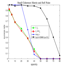
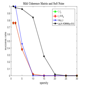
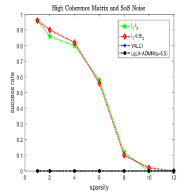
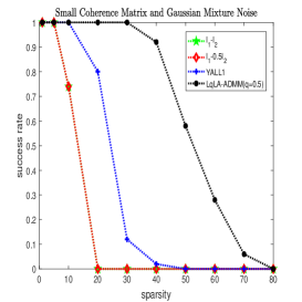
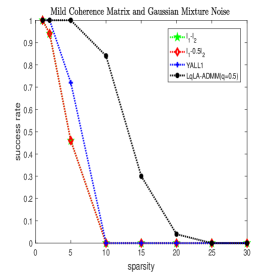
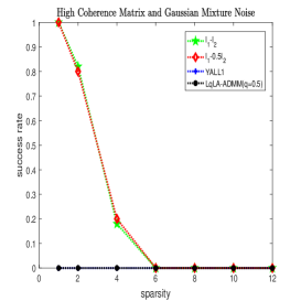
In our experiments, let $\bm{x}\in\bm{R}^{n}$ be a simulated $s$-sparse signal, where the support of $\bm{x}$ is a random index set and the $s$ non-zeros entries obey the Gaussian distribution $\mathcal{N}(0,1)$. we evaluate the compared methods using simulated sparse signals in various noise conditions. In addition, the signal $\bm{x}$ is normalized to have a unit energy value. Let $\bm{\hat{\bm{x}}}$ be a reconduction of $\bm{x}$ by apply each solver (YALL1 [58], LqLA-ADMM$(0<q<1)$ [52] and proposed $\ell_{1}-\alpha\ell_{2}$LA). If

$$\|\hat{\bm{x}}-\bm{x}\|_{2}/\|\bm{x}\|_{2}\leq 10^{-2},$$

the reconstruction is a success. Each provided result is an average over 100 independent Monte Carlo runs.

For both $S\tau S$ noise and Gaussian mixture noise, we respectively design three experiments. In the first experiment, the sensing matrix $\bm{A}\in\bm{R}^{m\times n}$ is orthonormal Gaussian random matrix with $m=128,n=256$, which has small coherence smaller than 0.35. In the second experiment, let $m=64$, $n=1280$ and the sensing matrix $\bm{A}\in\bm{R}^{m\times n}$ be orthonormal Gaussian random matrix, which has mild coherence between 0.5 and 0.65. In the third experiment, let the sensing matrix $\bm{A}\in\bm{R}^{m\times n}$ be oversampled partial DCT matrix with $m=32$ and $n=640$, and it has high coherence larger than 0.99.

Fig. 1 presents the successful rates of recovery for the YALL1, the LqLA-ADMM$(q=0.5)$ and the proposed $\ell_{1}-\alpha\ell_{2}$LA ($\alpha=1,0.5$) versus the sparsity $s$ in the $S\tau S$ noise case with $\tau=1$ (Cauchy noise) and $\gamma=10^{-4}$.In the left figure of Fig. 1, we observe the LqLA-ADMM$(q=0.5)$ has the best performance, followed by YALL1. In the middle figure of Fig. 1, the LqLA-ADMM$(q=0.5)$ still has the best performance. But, the difference between LqLA-ADMM$(q=0.5)$ and $\ell_{1}-\alpha\ell_{2}$LA becomes smaller. However, in the right figure, $\ell_{1}-\alpha\ell_{2}$-PLAD is the best and provides the robust performance regardless of large coherence of $\bm{A}$. And the LqLA-ADMM$(q=0.5)$ and YALL1 have lost efficiency.

And Fig. 2 presents the successful rates of recovery of the compared algorithms versus sparsity $s$ in Gaussian mixture noise with $\xi=0.1$ and $\kappa=1000$. In Fig. 2, we observe the same conclusions for this case as that in $S\tau S$ noise.

V-B MRI Reconstruction

In this subsection, we present a two-dimensional example of the reconstruction for MRI from a limited number of projections. It was first introduced in [8] to demonstrate the success of compressed sensing. The signal/image is a Shepp-Logan phantom of size $256\times 256$. See Fig. 3. In this case, the gradient of the signal is sparse. Thus [8, 35] proposed a model to minimize the (isotropic) total variation (TV) [43], i.e.,

$$\min\|\bm{u}\|_{TV}~{}~{}~{}\text{subject~{} to}~{}~{}\bm{R}\mathcal{F}\bm{u}=\bm{b},$$ (44)

where $\|\bm{u}\|_{TV}=\|\sqrt{|\mathcal{D}_{x}\bm{u}|^{2}+|\mathcal{D}_{y}\bm{u}|^{2}}\|_{1}$ with $\mathcal{D}_{x},\mathcal{D}_{y}$ respectively denoting the horizontal and vertical partial derivative operators, $\mathcal{F}$ is the Fourier transform, $\bm{R}$ is the sampling mask in the frequency space, and $\bm{b}$ is the data. It is claimed in [8] that 22 projections are necessary to achieve exact recovery. Later, some works suggest that imposing nonconvex metrices on gradients can achieve exact recovery from fewer numbers of projections, for example $\ell_{q}~{}(0<q<1)$ [14] using 10 projections, truncated $\ell_{1}$ [28] using 8 projections. More results about MRI reconstruction, readers can refer to [13, 39, 17, 40, 63] and so on.

Recently, Lou, et.al. [34] proposed the following weighted difference of convex regularization

$$\min \bigg{(}\|\mathcal{D}_{x}\bm{u}\|_{1}+\|\mathcal{D}_{y}\bm{u}\|_{1}-\alpha\Big{\|}\sqrt{|\mathcal{D}_{x}\bm{u}|^{2}+|\mathcal{D}_{y}\bm{u}|^{2}}\Big{\|}_{1}\bigg{)}$$

$$+\frac{\mu}{2}\|\bm{R}\mathcal{F}\bm{u}-\bm{b}\|_{2}^{2},$$ (45)

where $\alpha\in(0,1]$ is a parameter for a more general model. This model was called $\ell_{1}-\alpha\ell_{2}$-TV [34]. When $\alpha=1$, (V-B) is the $\ell_{1-2}$-TV model in [61]. These results of [61, 34] demonstrated that 8 projections are enough to guarantee exact recovery using $\ell_{1}-\alpha\ell_{2}$. However, this model is only fit for Gaussian noise. For impulsive noise, we consider the following model

$$\min \lambda\bigg{(}\|\mathcal{D}_{x}\bm{u}\|_{1}+\|\mathcal{D}_{y}\bm{u}\|_{1}-\alpha\Big{\|}\sqrt{|\mathcal{D}_{x}\bm{u}|^{2}+|\mathcal{D}_{y}\bm{u}|^{2}}\Big{\|}_{1}\bigg{)}$$

$$+\|\bm{R}\mathcal{F}\bm{u}-\bm{b}\|_{1},$$ (46)

where $\bm{b}=\bm{R}\mathcal{F}\bm{u}+\bm{z}$ with noise $\bm{z}\in\mathbb{R}^{n_{1}\times n_{2}}$. We call it as $\ell_{1}-\alpha\ell_{2}$TV-PLAD. Here, let impulsive noise be $S\tau S$ noise.

By ADMM and DCA algorithms, we present the special algorithm to compute (V-B). Splitting the term $\|\bm{R}\mathcal{F}\bm{u}-\bm{b}\|_{1}$, and respectively replacing $\mathcal{D}_{x}\bm{u},\mathcal{D}_{y}\bm{u}$ by $\bm{d}_{x},\bm{d}_{y}$, then one has an equivalent problem of (V-B) as follows

$$\min ~{}\lambda\bigg{(}\|\bm{d}_{x}\|_{1}+\|\bm{d}_{y}\|_{1}-\alpha\Big{\|}\sqrt{|\bm{d}_{x}|^{2}+|\bm{d}_{y}|^{2}}\Big{\|}_{1}\bigg{)}+\|\bm{v}\|_{1}$$

s. t. $$~{}\mathcal{D}_{x}\bm{u}=\bm{d}_{x},~{}\mathcal{D}_{y}\bm{u}=\bm{d}_{y},~{}\bm{R}\mathcal{F}\bm{u}-\bm{v}=\bm{b}.$$ (47)

Let

$$\mathcal{L}(\bm{u},\bm{v},\bm{d}_{x},\bm{d}_{y};\bm{w},\bm{h}_{x},\bm{h}_{y})$$

$$=\lambda\bigg{(}\|\bm{d}_{x}\|_{1}+\|\bm{d}_{y}\|_{1}-\alpha\Big{\|}\sqrt{|\bm{d}_{x}|^{2}+|\bm{d}_{y}|^{2}}\Big{\|}_{1}\bigg{)}+\|\bm{v}\|_{1}$$

$$\hskip 12.0pt+\frac{\rho_{1}}{2}\|\bm{R}\mathcal{F}\bm{u}-\bm{v}-\bm{b}\|_{2}^{2}-\langle\bm{w},\bm{R}\mathcal{F}\bm{u}-\bm{v}-\bm{b}\rangle$$

$$\hskip 12.0pt+\frac{\rho_{2}}{2}\|\mathcal{D}_{x}\bm{u}-\bm{d}_{x}\|_{2}^{2}-\langle\bm{h}_{x},\mathcal{D}_{x}\bm{u}-\bm{d}_{x}\rangle$$

$$\hskip 12.0pt+\frac{\rho_{2}}{2}\|\mathcal{D}_{y}\bm{u}-\bm{d}_{y}\|_{2}^{2}-\langle\bm{h}_{y},\mathcal{D}_{y}\bm{u}-\bm{d}_{y}\rangle$$

be the augmented Lagrangian function of (V-B) with the Lagrangian multipliers $\bm{w},\bm{h}_{x},\bm{h}_{y}\in\mathbb{R}^{n_{1}\times n_{2}}$. Then using ADMM iterate scheme and DCA in $\bm{d}_{x},\bm{d}_{y}$-subproblem, we give the special algorithm.

Algorithm 2 $\ell_{1}-\alpha\ell_{2}$LA for solving $\ell_{1}-\alpha\ell_{2}$TV-PLAD-(V-B)

Input  $\bm{R}$, $\bm{b}$, $0<\alpha\leq 1$, $\lambda$, $\rho_{1},\rho_{2}$.

Initialize

$(\bm{u},\bm{v},\bm{d}_{x},\bm{d}_{y};\bm{w},\bm{h}_{x},\bm{h}_{y})=(\bm{u}^{0},\bm{v}^{0},\bm{d}_{x}^{0},\bm{d}_{y}^{0};\bm{w}^{0},\bm{h}_{x}^{0},\bm{h}_{y}^{0})$,

$k=0$.

While  some stopping criterion is not satisfied do

1.  Compute sub-gradient $\bm{q}^{k}$ of $\|\sqrt{|\bm{d}_{x}|^{2}+|\bm{d}_{y}|^{2}}\|_{1}$ at point

$(\bm{d}_{x}^{k},\bm{d}_{y}^{k})$ by

$\bm{q}^{k}=(\bm{q}_{x}^{k};\bm{q}_{y}^{k})=\frac{(\bm{d}_{x}^{k};\bm{d}_{y}^{k})}{\sqrt{|\bm{d}_{x}^{k}|^{2}+|\bm{d}_{y}^{k}|^{2}}}$

2.   Compute $\bm{u}^{k+1}$ by

$\bm{u}^{k+1}=\big{(}\rho_{1}\bm{R}^{T}\bm{R}-\rho_{2}\mathcal{\triangle}\big{)}^{-1}\bigg{(}\rho_{1}\mathcal{F}^{*}\bm{R}(\bm{b}+\bm{v}^{k}+\bm{w}^{k})$

$+\rho_{2}\mathcal{D}_{x}^{T}(\bm{d}_{x}^{k}+\bm{h}_{x}^{k})+\rho_{2}\mathcal{D}_{y}^{T}(\bm{d}_{y}^{k}+\bm{h}_{y}^{k})\bigg{)}.$

3.  Compute $\bm{v}^{k+1}$ by

$\bm{v}^{k+1}=S(\bm{R}\mathcal{F}\bm{u}^{k+1}-\bm{b}-\bm{w}^{k},\frac{1}{\rho_{1}})$.

4.  Update $\bm{d}_{x}^{k+1},~{}\bm{d}_{y}^{k+1}$ via

$\bm{d}_{x}^{k+1}=S\bigg{(}(\mathcal{D}_{x}\bm{u}^{k+1}-\bm{h}_{x}^{k})+\frac{\lambda\alpha}{\rho_{2}}\bm{q}_{x}^{k},\frac{\lambda}{\rho_{2}}\bigg{)}$,

$\bm{d}_{y}^{k+1}=S\bigg{(}(\mathcal{D}_{y}\bm{u}^{k+1}-\bm{h}_{y}^{k})+\frac{\lambda\alpha}{\rho_{2}}\bm{q}_{y}^{k},\frac{\lambda}{\rho_{2}}\bigg{)}$.

5.  Update dual variables

$\bm{w}^{k+1}=\bm{w}^{k}-\rho_{1}(\bm{R}\mathcal{F}\bm{u}^{k+1}-\bm{v}^{k+1}-\bm{b})$

$\bm{h}_{x}^{k+1}=\bm{h}_{x}^{k}-\rho_{2}(\mathcal{D}_{x}\bm{u}^{k+1}-\bm{d}_{x}^{k+1})$

$\bm{h}_{y}^{k+1}=\bm{h}_{y}^{k}-\rho_{2}(\mathcal{D}_{y}\bm{u}^{k+1}-\bm{d}_{y}^{k+1})$.

6.  $k=k+1$.

End

Remark 6.

In Algorithm 2, $\alpha$ is a model parameter and satisfies $0<\alpha\leq 1$, $\lambda>0$ is a penalty parameter, $0<\rho_{1},~{}\rho_{2}<1$ are regularized parameters.

In this section, numerical experiments compare our $\ell_{1}-\alpha\ell_{2}$LA algorithm with some other efficient methods including YALL1 [58] for penalized LAD model

$$\min~{}\lambda(\|\mathcal{D}_{x}\bm{u}\|_{1}+\|\mathcal{D}_{y}\bm{u}\|_{1})+\|\bm{R}\mathcal{F}\bm{u}-\bm{b}\|_{1}$$ (48)

and LqLA-ADMM [52]

$$\min~{}\lambda(\|\mathcal{D}_{x}\bm{u}\|_{q}^{q}+\|\mathcal{D}_{y}\bm{u}\|_{q}^{q})+\|\bm{R}\mathcal{F}\bm{u}-\bm{b}\|_{1,\varepsilon},$$ (49)

where $0<q<1$.

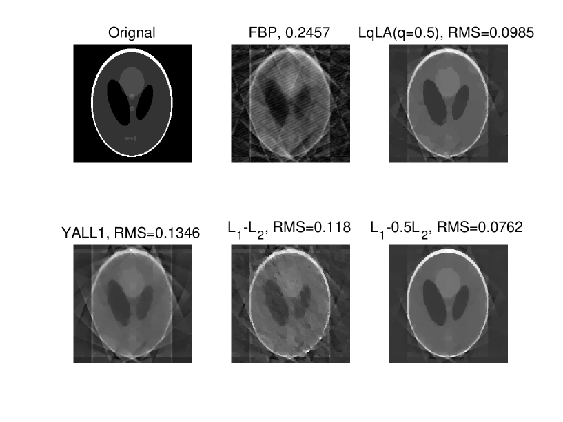
Fig. 3 shows the stable recovery of 8 projections using the proposed method. In Fig. 3, the root-mean-square (RMS) error is used to measure the performance quantitatively. The RMS between reference and distorted images $\bm{X}$, $\bm{Y}$ is defined as $\text{RMS}(\bm{X},\bm{Y})=\|\bm{X}-\bm{Y}\|_{2}/\sqrt{M}$, where $M$ is the number of pixels in images $\bm{X}$,$\bm{Y}$. Figure 3 explains that $\ell_{1}-\alpha\ell_{2}~{}(\alpha=0.5)$ is much better than YALL1 and LqLA-ADMM $(q=0.5)$ visually as well as in terms of RMS. Fig. 3 also shows that 8 projections are sufficient to have stable recovery in impulsive noise by using the $\ell_{1}-\alpha\ell_{2}$LA method.

Figure 3: MRI reconstruction from observation with impulsive noise. It is demonstrated that 8 projections are enough to have stable recovery in impulsive using $L_{1}-\alpha L_{2}$LA. The root-mean-square (RMS) errors are provided for each method.

VI Conclusions

In this paper, we consider the signal and image reconstructions in impulsive noise via $\ell_{1}-\alpha\ell_{2}~{}(0<\alpha\leq 1)$ minimization. First, we propose the two new models of $\ell_{1}-\alpha\ell_{2}$-LAD (12), and $\ell_{1}-\alpha\ell_{2}$-DS (15) in Section I. In Section II, we obtain a sufficient condition based on $(\ell_{2},\ell_{1})$-RIP to guarantee the exact recovery of $\bm{x}$ from $\bm{b}=\bm{A}\bm{x}$ via (16) (see Theorem 1)). And in Section III, we consider the recovery of $\bm{x}$ via (12) and (15) in the noisy case. We give the sufficient $(\ell_{2},\ell_{1})$-RIP conditions to guarantee the stable recovery of $\bm{x}$ from $\bm{b}=\bm{A}\bm{x}+\bm{z}$ (see Theorem 2 and Theorem 3).

In order to obtain the efficient algorithm of (12), we introduce the unconstrained $\ell_{1}-\alpha\ell_{2}$ model $\ell_{1}-\alpha\ell_{2}$-PLAD (13). Using ADMM and DCA, we have developed a numerical scheme-$\ell_{1}-\alpha\ell_{2}$LA to efficiently solve our unconstrained problem (13) in section IV.

Last, we present numerical experiments for the sparse signal and compressible image recovery in impulsive noise case. They demonstrate the efficiency of $\ell_{1}-\alpha\ell_{2}$LA method (see section V). In signal recovery experiments, let sensing matrix $\bm{A}$ has different coherence: small coherence $\mu(\bm{A})<0.35$, mild coherence $0.5<\mu(\bm{A})<0.65$ and high coherence $\mu(\bm{A})>0.99$. Although our method performs not well when sensing matrix has small coherence, the difference is smaller when the coherence increases. And when the measurement matrix has high coherence, our method becomes the best. And the MRI phantom image recovery test also demonstrates that $\ell_{1}-\alpha\ell_{2}$LA is highly effective and comparable to state-of-the-art methods.

Appendix A Proof of Theorem 1

Proof.

Let $\hat{\bm{x}}$ be the minimizer of (16). Clearly, $\bm{b}=\bm{A}\hat{\bm{x}}$ and $\|\hat{\bm{x}}\|_{\alpha,1-2}\leq\|\bm{x}\|_{\alpha,1-2}$. Let $\bm{h}=\hat{\bm{x}}-\bm{x}$. Suppose that $\bm{h}\in\mathcal{N}(\bm{A})\backslash\{\bm{0}\}$. Then by (20) in Lemma 1, we have

$$\|\bm{h}_{-\max(s)}\|_{1}\leq\|\bm{h}_{\max(s)}\|_{1}+\alpha\|\bm{h}\|_{2}.$$ (50)

From $\bm{b}=\bm{Ax}$ and $\bm{b}=\bm{A}\hat{\bm{x}}$, it follows that

$$\|\bm{Ah}\|_{1}=\|\bm{A}\hat{\bm{x}}-\bm{Ax}\|_{1}=\bm{0}.$$ (51)

Let $T_{0}=\text{supp}(\bm{h}_{\max(s)})$, $t=ks\in\mathbb{Z}_{+}$, $T_{1}$ be the index set of the $t\in\mathbb{Z}_{+}$ largest entries of $\bm{h}_{-\max(s)}$ and $T_{01}=T_{0}\cup T_{1}$. Thus, by the facts that $\bm{A}$ satisfies the $(\ell_{2},\ell_{1})$-RIP condition of $(k+1)s$ order, $t=ks$, $\bm{x}$ is $s$-sparse and Lemma 3, ones have a lower bound of $\|\bm{Ah}\|_{1}$

$$\|\bm{Ah}\|_{1} \geq\rho_{ks}\|\bm{h}_{T_{01}}\|_{2},$$ (52)

where $\rho_{ks}=1-\delta_{(k+1)s}^{lb}-\frac{(1+\delta_{ks}^{ub})}{a(s,ks;\alpha)}$ with $a(s,ks;\alpha)=\frac{\sqrt{ks}-\alpha}{\sqrt{s}+\alpha}>1.$

Combining the lower bound (52) with (51), we have

$$0\geq\Big{(}1-\delta_{(k+1)s}^{lb}-\frac{1+\delta_{ks}^{ub}}{a(s,ks;\alpha)}\Big{)}\|\bm{h}_{T_{01}}\|_{2}.$$ (53)

Note that the condition (29) implies that

$$1-\delta_{(k+1)s}^{lb}-\frac{1+\delta_{ks}^{ub}}{a(s,ks;\alpha)}>0,$$

i.e., $\rho_{ks}>0$. Then by (53), it is clear that

$$\|\bm{h}_{T_{01}}\|_{2}\leq 0,$$

Therefore, by the definition of $T_{01}$, $\bm{h}=\bm{0}$, which contradicts with the assumption $\bm{h}\in\mathcal{N}(\bm{A})\backslash\{\bm{0}\}$. We complete the proof. ∎

Appendix B Proof of Theorem 2

Proof.

Let $\bm{h}=\hat{\bm{x}}^{\ell_{1}}-\bm{x}$. Since $\hat{\bm{x}}^{\ell_{1}}$ is the minimizer of (12), $\|\bm{b}-\bm{A}\hat{\bm{x}}^{\ell_{1}}\|_{1}\leq\eta_{1}$ and $\|\hat{\bm{x}}^{\ell_{1}}\|_{\alpha,1-2}\leq\|\bm{x}\|_{\alpha,1-2}$. Then, by (19) in Lemma 1, we have

$$\|\bm{h}_{-\max(s)}\|_{1}\leq\|\bm{h}_{\max(s)}\|_{1}+2\|\bm{x}_{-\max(s)}\|_{1}+\alpha\|\bm{h}\|_{2}.$$ (54)

By the facts that $\|\bm{z}\|_{1}=\|\bm{b}-\bm{Ax}\|_{1}\leq\eta_{1}$ and $\|\bm{b}-\bm{A}\hat{\bm{x}}^{\ell_{1}}\|_{1}\leq\eta_{1}$, one has

$$\|\bm{Ah}\|_{1}=\|\bm{A}\hat{\bm{x}}^{\ell_{1}}-\bm{Ax}\|_{1}\leq \|\bm{A}\hat{\bm{x}}^{\ell_{1}}-\bm{b}\|_{1}$$

$$+\|\bm{b}-\bm{Ax}\|_{1}\leq \eta_{1}+\eta_{1}=2\eta_{1}.$$ (55)

Similar to the proof of Theorem 1, let $T_{0}=\text{supp}(\bm{h}_{\max(s)})$, $t=ks\in\mathbb{Z}_{+}$, $T_{1}$ be the index set of the $t=ks$ largest entries of $\bm{h}_{-\max(s)}$ and $T_{01}=T_{0}\cup T_{1}$. Thus, by the facts that $\bm{A}$ satisfies the $(\ell_{2},\ell_{1})$-RIP condition of $(k+1)s$ order, $t=ks$, and Lemma 3, ones obtain a lower bound of $\|\bm{Ah}\|_{1}$

$$\|\bm{Ah}\|_{1}\geq \rho_{ks}\|\bm{h}_{T_{01}}\|_{2}-(1+\delta_{ks}^{ub})\frac{2\|\bm{x}_{-\max(s)}\|_{1}}{\sqrt{ks}-\alpha},$$ (56)

where $\rho_{ks}=1-\delta_{(k+1)s}^{lb}-\frac{(1+\delta_{ks}^{ub})}{a(s,ks;\alpha)}$ with $a(s,ks;\alpha)=\frac{\sqrt{ks}-\alpha}{\sqrt{s}+\alpha}$.

By (56) and (B), we have

$$2\eta_{1}\geq \Big{(}1-\delta_{(k+1)s}^{lb}-\frac{(1+\delta_{ks}^{ub})}{a(s,ks;\alpha)}\Big{)}\|\bm{h}_{T_{01}}\|_{2}$$

$$-(1+\delta_{ks}^{ub})\frac{2\|\bm{x}_{-\max(s)}\|_{1}}{\sqrt{ks}-\alpha}.$$ (57)

where $a(s;ks,\alpha)=\frac{\sqrt{ks}-\alpha}{\sqrt{s}+\alpha}>1$. Furthermore, the condition (29) implies that

$$1-\delta_{(k+1)s}^{lb}-\frac{(1+\delta_{ks}^{ub})}{a(s,ks;\alpha)}>0,$$

that is $\rho_{ks}>0$. Then, by (B), one has

$$\|\bm{h}_{T_{01}}\|_{2}\leq\frac{2}{\rho_{ks}}\eta_{1}+\frac{(1+\delta_{ks}^{ub})\sqrt{s}}{(\sqrt{ks}-\alpha)\rho_{ks}}\frac{2\|\bm{x}_{-\max(s)}\|_{1}}{\sqrt{s}}.$$ (58)

By the fact that $\|\bm{h}\|_{2}=\sqrt{\|\bm{h}_{T_{01}}\|_{2}^{2}+\|\bm{h}_{T_{01}^{c}}\|_{2}^{2}}$, to show (2), we need to estimate the upper bound of $\|\bm{h}_{T_{01}^{c}}\|_{2}$. Without loss of generality, we assume that $|h_{1}|\geq\cdots\geq|h_{s}|\geq|h_{s+1}|\geq\cdots\geq|h_{s+t}|\geq\cdots\geq|h_{n}|$ with $t=ks\in\mathbb{Z}_{+}$. Then,

$$\|\bm{h}_{T_{01}^{c}}\|_{2}\leq \sqrt{\|\bm{h}_{T_{01}^{c}}\|_{1}\|\bm{h}_{T_{01}^{c}}\|_{\infty}}$$

$$\overset{(1)}{\leq} \sqrt{\Big{(}\|\bm{h}_{T_{0}^{c}}\|_{1}-\sum_{j\in T_{1}}|h_{j}|\Big{)}|h_{s+t}|}$$

$$\overset{(2)}{\leq} \sqrt{\Big{(}\|\bm{h}_{T_{0}^{c}}\|_{1}-t|h_{s+t}|\Big{)}|h_{s+t}|}$$

$$= \sqrt{-t\Big{(}|h_{s+t}|-\frac{\|\bm{h}_{T_{0}^{c}}\|_{1}}{2t}\Big{)}^{2}+\frac{\|\bm{h}_{T_{0}^{c}}\|_{1}^{2}}{4t}}$$

$$\leq\frac{\|\bm{h}_{T_{0}^{c}}\|_{1}}{2\sqrt{t}}$$

$$\overset{(3)}{\leq} \frac{\|\bm{h}_{\max(s)}\|_{1}+2\|\bm{x}_{-\max(s)}\|_{1}+\alpha\|\bm{h}\|_{2}}{2\sqrt{t}}$$

$$\overset{(4)}{\leq} \frac{1}{2}\sqrt{\frac{s}{t}}\Big{(}\|\bm{h}_{T_{01}}\|_{2}+\frac{2\|\bm{x}_{-\max(s)}\|_{1}+\alpha\|\bm{h}\|_{2}}{\sqrt{s}}\Big{)}$$

$$\overset{(5)}{=} \frac{1}{2\sqrt{k}}\bigg{(}\|\bm{h}_{T_{01}}\|_{2}+\frac{2\|\bm{x}_{-\max(s)}\|_{1}+\alpha\|\bm{h}\|_{2}}{\sqrt{s}}\bigg{)},$$ (59)

where (1) and (2) are from $T_{01}=T_{0}\cup T_{1}$, $|T_{1}|=t$ and the assumption $|h_{1}|\geq\cdots\geq|h_{s}|\geq|h_{s+1}|\geq\cdots\geq|h_{s+t}|\geq\cdots\geq|h_{n}|$, (3) follows from (54), (4) is due to $\|\bm{h}_{\max(s)}\|_{1}\leq\sqrt{s}\|\bm{h}_{\max(s)}\|_{2}$, $T_{0}=\mathrm{supp}(\bm{h}_{\max(s)})$ and $T_{01}=T_{0}\cup T_{1}$, and (5) follows from $t=ks\in\mathbb{Z}_{+}$.

By (B), ones have

$$\|\bm{h}\|_{2}=\sqrt{\|\bm{h}_{T_{01}}\|_{2}^{2}+\|\bm{h}_{T_{01}^{c}}\|_{2}^{2}}$$

$$\leq\sqrt{\|\bm{h}_{T_{01}}\|_{2}^{2}+\frac{1}{4k}\bigg{(}\|\bm{h}_{T_{01}}\|_{2}+\frac{2\|\bm{x}_{-\max(s)}\|_{1}+\alpha\|\bm{h}\|_{2}}{\sqrt{s}}\bigg{)}^{2}}$$

$$\leq\bigg{(}1+\frac{1}{2\sqrt{k}}\bigg{)}\|\bm{h}_{T_{01}}\|_{2}+\frac{1}{2\sqrt{k}}\frac{2\|\bm{x}_{-\max(s)}\|_{1}}{\sqrt{s}}+\frac{1}{2\sqrt{k}}\frac{\alpha\|\bm{h}\|_{2}}{\sqrt{s}},$$ (60)

where the last inequality is due to the basic inequality $\sqrt{a^{2}+b^{2}}\leq a+b$ for $a,b\geq 0$. Since $0\leq\alpha\leq 1$ and $ks\in\mathbb{Z}_{+}$, $1-\frac{\alpha}{2\sqrt{ks}}>0$. Thus, based on (B), we have

$$\|\bm{h}\|_{2}\leq\frac{(2\sqrt{k}+1)\sqrt{s}}{2\sqrt{ks}-\alpha}\|\bm{h}_{T_{01}}\|_{2}+\frac{\sqrt{s}}{2\sqrt{ks}-\alpha}\frac{2\|\bm{x}_{-\max(s)}\|_{1}}{\sqrt{s}}.$$

Substituting (58) into the above inequality, ones get

$$\|\bm{h}\|_{2}\leq\frac{(2\sqrt{k}+1)\sqrt{s}}{2\sqrt{ks}-\alpha}\Big{(}\frac{2}{\rho_{ks}}\eta_{1}+\frac{(1+\delta_{ks}^{ub})\sqrt{s}}{\rho_{ks}(\sqrt{ks}-\alpha)}\frac{2\|\bm{x}_{-\max(s)}\|_{1}}{\sqrt{s}}\Big{)}$$

$$\ \ +\frac{\sqrt{s}}{2\sqrt{ks}-\alpha}\frac{2\|\bm{x}_{-\max(s)}\|_{2}}{\sqrt{s}}$$

$$=\frac{\sqrt{s}}{2\sqrt{ks}-\alpha}\Big{(}\frac{(2\sqrt{k}+1)(1+\delta_{ks}^{ub})\sqrt{s}}{\rho_{ks}(\sqrt{ks}-\alpha)}+1\Big{)}\frac{2\|\bm{x}_{-\max(s)}\|_{1}}{\sqrt{s}}$$

$$+\frac{2(2\sqrt{k}+1)\sqrt{s}}{(2\sqrt{2}\sqrt{s}-\alpha)\rho_{ks}}\eta_{1}.$$

We complete the proof of Theorem 2. ∎

Appendix C Proof of Theorem 3

Proof.

Take $\bm{h}=\hat{\bm{x}}^{DS}-\bm{x}$. Since $\hat{\bm{x}}^{DS}$ is the minimizer of (15), which implies $\|\hat{\bm{x}}^{DS}\|_{\alpha,1-2}\leq\|\bm{x}\|_{\alpha,1-2}$ and $\|\bm{A}^{*}(\bm{b}-\bm{A}\hat{\bm{x}}^{DS})\|_{\infty}\leq\eta_{2}$, (54) still holds. From the facts $\|\bm{A}^{*}\bm{z}\|_{\infty}=\|\bm{A}^{*}(\bm{b}-\bm{Ax})\|_{\infty}\leq\eta_{2}$ and $\|\bm{A}^{*}(\bm{b}-\bm{A}\hat{\bm{x}}^{DS})\|_{\infty}\leq\eta_{2}$, we have the following tube constraint inequality

$$\|\bm{A}^{*}\bm{Ah}\|_{\infty}= \|\bm{A}^{*}(\bm{A}^{*}{\bm{x}}^{DS}-\bm{Ax)}\|_{\infty}$$

$$\leq \|\bm{A}^{*}(\bm{A}\hat{\bm{x}}^{DS}-\bm{b})\|_{\infty}+\|\bm{A}^{*}(\bm{b}-\bm{Ax})\|_{\infty}$$

$$\leq \eta_{2}+\eta_{2}=2\eta_{2}$$ (61)

instead of (B).

Similarly, let $T_{0}=\text{supp}(\bm{h}_{\max(s)})$, $t=ks\in\mathbb{Z}_{+}$, $T_{1}$ be the index set of the $t\in\mathbb{Z}_{+}$ largest entries of $\bm{h}_{-\max(s)}$ and $T_{01}=T_{0}\cup T_{1}$. Since $\bm{A}$ satisfies the $(\ell_{2},\ell_{1})$-RIP condition of $(k+1)s$ order, $t=ks$, and Lemma 3, (56) holds, which presents a lower bound of $\|\bm{Ah}\|_{1}$.

Next, we estimate the upper bound of $\|\bm{Ah}\|_{1}$ using new technology, which is completely different from that of the proof for Theorem 2.

By Cauchy-Schwartz inequality, we have

$$\|\bm{Ah}\|_{1} \leq\sqrt{m}\|\bm{Ah}\|_{2}=\sqrt{m}\langle\bm{Ah},\bm{Ah}\rangle^{1/2}$$

$$=\sqrt{m}\langle\bm{A}^{*}\bm{Ah},\bm{h}\rangle^{1/2}\leq\sqrt{m}\sqrt{\|\bm{A}^{*}\bm{Ah}\|_{\infty}\|\bm{h}\|_{1}}$$

$$=\sqrt{m}\sqrt{\|\bm{A}^{*}\bm{Ah}\|_{\infty}(\|\bm{h}_{T_{0}}\|_{1}+\|\bm{h}_{T_{0}^{c}}\|_{1})}$$

$$\overset{(1)}{\leq}\sqrt{m}\sqrt{2\eta_{2}(2\|\bm{h}_{T_{0}}\|_{1}+2\|\bm{x}_{-\max(s)}\|_{1}+\alpha\|\bm{h}\|_{2})}$$

$$\overset{(2)}{\leq}\sqrt{2m\sqrt{s}\eta_{2}\bigg{(}2\|\bm{h}_{T_{01}}\|_{2}+\frac{2\|\bm{x}_{-\max(s)}\|_{1}+\alpha\|\bm{h}\|_{2}}{\sqrt{s}}\bigg{)}}$$ (62)

where (1) is from (C), (2) is due to $T_{01}=T_{0}\cup T_{1}$ and $\|\bm{h}_{T_{0}}\|_{1}\leq\sqrt{s}\|\bm{h}_{T_{0}}\|_{2}$ with $|T_{0}|\leq s$.

Combining (56) with (C), we have

$$\rho_{ks}\|\bm{h}_{T_{01}}\|_{2}-\frac{(1+\delta_{ks}^{ub})\sqrt{s}}{\sqrt{ks}-\alpha}\frac{2\|\bm{x}_{-\max(s)}\|_{1}}{\sqrt{s}}$$

$$\leq\sqrt{2m\sqrt{s}\eta_{2}\bigg{(}2\|\bm{h}_{T_{01}}\|_{2}+\frac{2\|\bm{x}_{-\max(s)}\|_{1}+\alpha\|\bm{h}\|_{2}}{\sqrt{s}}\bigg{)}},$$ (63)

where $\rho_{ks}=1-\delta_{t+s}^{lb}-\frac{(1+\delta_{ks}^{ub})}{a(s,ks;\alpha)}$ with $a(s,ks;\alpha)=\frac{\sqrt{ks}-\alpha}{\sqrt{s}+\alpha}>1$. Furthermore,

$$1-\delta_{(k+1)s}^{lb}-\frac{1+\delta_{ks}^{ub}}{a(s,ks;\alpha)}$$

$$>1-\delta_{(k+1)s}^{lb}-\frac{(1+b(s,k;\alpha))(1+\delta_{ks}^{ub})}{a(s,ks;\alpha)b(s,k;\alpha)}>0$$

where the first and last inequalities are from $b(s,k;\alpha)=\frac{8(2\sqrt{ks}-\alpha)}{17\alpha(2\sqrt{k}+1)}>0$ with $0<\alpha\leq 1$ and $\eqref{RIPCondition3}$, respectively.

To estimate $\|\bm{h}_{T_{01}}\|_{2}$ from (C), we consider the following two cases.

First, if

$$\rho_{ks}\|\bm{h}_{T_{01}}\|_{2}-\frac{(1+\delta_{ks}^{ub})\sqrt{s}}{\sqrt{ks}-\alpha}\frac{2\|\bm{x}_{-\max(s)}\|_{1}}{\sqrt{s}}<0,$$

i.e.,

$$\|\bm{h}_{T_{01}}\|_{2}<\frac{(1+\delta_{ks}^{ub})\sqrt{s}}{(\sqrt{ks}-\alpha)\rho_{ks}}\frac{2\|\bm{x}_{-\max(s)}\|_{1}}{\sqrt{s}}.$$

Second, if

$$\Big{(}1- \delta_{t+s}^{lb}-\frac{1+\delta_{ks}^{ub}}{a(s;ks,\alpha)}\Big{)}\|\bm{h}_{T_{01}}\|_{2}$$

$$\hskip 12.0pt-\frac{(1+\delta_{ks}^{ub})\sqrt{s}}{\sqrt{ks}-\alpha}\frac{2\|\bm{x}_{-\max(s)}\|_{1}}{\sqrt{s}}\geq 0,$$

which implies

$$\|\bm{h}_{T_{01}}\|_{2}\geq\frac{(1+\delta_{ks}^{ub})\sqrt{s}}{(\sqrt{ks}-\alpha)\rho_{ks}}\frac{2\|x_{-\max(s)}\|_{1}}{\sqrt{s}},$$

then the inequality (C) is equivalent to

$$\bigg{(}\rho_{ks}\|\bm{h}_{T_{01}}\|_{2}-\frac{(1+\delta_{ks}^{ub})\sqrt{s}}{\sqrt{ks}-\alpha}\frac{2\|\bm{x}_{-\max(s)}\|_{1}}{\sqrt{s}}\bigg{)}^{2}$$

$$\leq 2m\sqrt{s}\eta_{2}\bigg{(}2\|\bm{h}_{T_{01}}\|_{2}+\frac{2\|\bm{x}_{-\max(s)}\|_{1}+\alpha\|\bm{h}\|_{2}}{\sqrt{s}}\bigg{)}.$$ (64)

Let $X=\|\bm{h}_{T_{01}}\|_{2}$ and $Y=\frac{2\|\bm{x}_{-\max(s)}\|_{1}+\alpha\|h\|_{2}}{\sqrt{s}}$. By $\frac{2\|\bm{x}_{-\max(s)}\|_{1}}{\sqrt{s}}\leq Y$, to guarantee that (C) holds, it suffices to show

$$\rho_{ks}^{2}X^{2}-\bigg{(}\frac{2\rho_{1}(1+\delta_{ks}^{ub})\sqrt{s}}{\sqrt{ks}-\alpha}Y+4m\sqrt{s}\eta_{2}\bigg{)}X$$

$$-2m\sqrt{s}\eta_{2}Y\leq 0.$$ (65)

For the one-variable quadratic inequality $aZ^{2}-bZ-c\leq 0$ with the constants $a,b,c>0$, there is the fact that

$$Z\leq\frac{b+\sqrt{b^{2}+4ac}}{2a}\leq\frac{b}{a}+\sqrt{\frac{c}{a}}.$$

Hence,

$$X\leq \frac{2\rho_{ks}\frac{(1+\delta_{ks}^{ub})\sqrt{s}}{\sqrt{ks}-\alpha}Y+4m\sqrt{s}\eta_{2}}{\rho_{ks}^{2}}+\sqrt{\frac{2m\sqrt{s}\eta_{2}\varepsilon Y}{\rho_{ks}^{2}\varepsilon}}$$

$$\leq \frac{2(1+\delta_{ks}^{ub})\sqrt{s}}{(\sqrt{ks}-\alpha)\rho_{ks}}Y+\frac{4m\sqrt{s}}{\rho_{ks}^{2}}\eta_{2}+\frac{1}{2}\bigg{(}\frac{2m\sqrt{s}}{\rho_{ks}^{2}\varepsilon}\eta_{2}+\varepsilon Y\bigg{)}$$

$$= \bigg{(}\frac{2(1+\delta_{ks}^{ub})\sqrt{s}}{(\sqrt{ks}-\alpha)\rho_{ks}}+\frac{\varepsilon}{2}\bigg{)}Y+\bigg{(}4+\frac{1}{\varepsilon}\bigg{)}\frac{m\sqrt{s}}{\rho_{ks}^{2}}\eta_{2},$$ (66)

where $\varepsilon>0$ is to be determined later.

By the above discussion and

$$\bigg{(}\frac{2(1+\delta_{ks}^{ub})\sqrt{s}}{(\sqrt{ks}-\alpha)\rho_{ks}}+\frac{\varepsilon}{2}\bigg{)}Y+\bigg{(}4+\frac{1}{\varepsilon}\bigg{)}\frac{m\sqrt{s}}{\rho_{ks}^{2}}\eta_{2}$$

$$=\bigg{(}\frac{2(1+\delta_{ks}^{ub})\sqrt{s}}{(\sqrt{ks}-\alpha)\rho_{1}}+\frac{\varepsilon}{2}\bigg{)}\frac{2\|\bm{x}_{-\max(s)}\|_{1}+\alpha\|\bm{h}\|_{2}}{\sqrt{s}}$$

$$\hskip 12.0pt+\bigg{(}4+\frac{1}{\varepsilon}\bigg{)}\frac{m\sqrt{s}}{\rho_{1}^{2}}\eta_{2}$$

$$\geq\frac{(1+\delta_{ks}^{ub})\sqrt{s}}{(\sqrt{ks}-\alpha)\rho_{ks}}\frac{2\|\bm{x}_{-\max(s)}\|_{1}}{\sqrt{s}},$$

the inequality (C) always holds when

$$\|\bm{h}_{T_{01}}\|_{2}\leq \bigg{(}\frac{2(1+\delta_{ks}^{ub})\sqrt{s}}{(\sqrt{ks}-\alpha)\rho_{ks}}+\frac{\varepsilon}{2}\bigg{)}\frac{2\|\bm{x}_{-\max(s)}\|_{1}+\alpha\|\bm{h}\|_{2}}{\sqrt{s}}$$

$$+\bigg{(}4+\frac{1}{\varepsilon}\bigg{)}\frac{m\sqrt{s}}{\rho_{ks}^{2}}\eta_{2},$$ (67)

which presents an upper bound $\|\bm{h}_{T_{01}}\|_{2}$.

Next, we will estimate $\|\bm{h}_{T_{01}^{c}}\|_{2}$. In terms of the derivations of (B) and (B), they still hold.

Substituting (C) into (B), ones obtain

$$\|\bm{h}\|_{2}\leq\bigg{(}1+\frac{1}{2\sqrt{k}}\bigg{)}\Bigg{(}\bigg{(}4+\frac{1}{\varepsilon}\bigg{)}\frac{m\sqrt{s}}{\rho_{ks}^{2}}\eta_{2}$$

$$\hskip 12.0pt+\bigg{(}\frac{2(1+\delta_{ks}^{ub})\sqrt{s}}{(\sqrt{ks}-\alpha)\rho_{ks}}+\frac{\varepsilon}{2}\bigg{)}\frac{2\|\bm{x}_{-\max(s)}\|_{1}+\alpha\|\bm{h}\|_{2}}{\sqrt{s}}\Bigg{)}$$

$$\hskip 12.0pt+\frac{1}{2\sqrt{k}}\frac{2\|\bm{x}_{-\max(s)}\|_{1}}{\sqrt{s}}+\frac{\alpha}{2\sqrt{k}}\frac{\|\bm{h}\|_{2}}{\sqrt{s}}$$

$$\leq\frac{1}{2\sqrt{k}}\Bigg{(}(2\sqrt{k}+1)\bigg{(}\frac{2(\sqrt{s}+\alpha)(1+\delta_{ks}^{ub})}{(\sqrt{ks}-\alpha)\rho_{ks}}+\frac{\varepsilon}{2}\bigg{)}+1\Bigg{)}$$

$$\hskip 24.0pt\times\frac{2\|\bm{x}_{-\max(s)}\|_{1}}{\sqrt{s}}$$

$$\hskip 12.0pt+\frac{1}{2\sqrt{k}}\Bigg{(}(2\sqrt{k}+1)\bigg{(}\frac{2(\sqrt{s}+\alpha)(1+\delta_{ks}^{ub})}{(\sqrt{ks}-1)\rho_{ks}}+\frac{\varepsilon}{2}\bigg{)}+1\Bigg{)}$$

$$\hskip 24.0pt\times\frac{\alpha\|\bm{h}\|_{2}}{\sqrt{s}}$$

$$\hskip 12.0pt+\bigg{(}1+\frac{1}{2\sqrt{k}}\bigg{)}\bigg{(}4+\frac{1}{\varepsilon}\bigg{)}\frac{m\sqrt{s}}{\rho_{ks}^{2}}\eta_{2}$$

$$=\varrho\frac{2\|\bm{x}_{-\max(s)}\|_{1}}{\sqrt{s}}+\frac{\alpha\varrho}{\sqrt{s}}\|\bm{h}\|_{2}$$

$$\hskip 12.0pt+\bigg{(}4+\frac{1}{\varepsilon}\bigg{)}\frac{(2\sqrt{k}+1)m\sqrt{s}}{2\sqrt{k}\rho_{1}^{2}}\eta_{2},$$

where the last equality is from

$$\varrho=\frac{1}{2\sqrt{k}}\Bigg{(}(2\sqrt{k}+1)\bigg{(}\frac{2(1+\delta_{ks}^{ub})}{a(s,ks;\alpha)\rho_{ks}}+\frac{\varepsilon}{2}\bigg{)}+1\Bigg{)}.$$

Taking

$$\varepsilon=\frac{2(1+\delta_{ks}^{ub})}{8a(s,ks;\alpha)\rho_{ks}},$$

then

$$\varrho=\frac{1}{2\sqrt{k}}\Bigg{(}(2\sqrt{k}+1)\frac{17(1+\delta_{ks}^{ub})}{16a(s,ks;\alpha)\rho_{ks}}+1\Bigg{)}<\frac{\sqrt{s}}{\alpha},$$ (68)

where the last inequality is from (3). In fact,

$$\varrho-\frac{\sqrt{s}}{\alpha}=\frac{1}{2\sqrt{k}}\Bigg{(}(2\sqrt{k}+1)\frac{3(1+\delta_{ks}^{ub})}{a(s,ks;\alpha)\rho_{ks}}+1\Bigg{)}-\frac{\sqrt{s}}{\alpha}$$

$$=\frac{17(2\sqrt{k}+1)}{16\sqrt{k}a(s,ks;\alpha)\rho_{ks}}$$

$$\hskip 12.0pt\Bigg{(}1+\delta_{ks}^{ub}-\bigg{(}1-\frac{2\sqrt{ks}}{\alpha}\bigg{)}\frac{8}{17(2\sqrt{k}+1)}a(s,ks;\alpha)\rho_{ks}\Bigg{)}$$

$$=:\frac{17(2\sqrt{k}+1)}{16\sqrt{k}a(s,ks;\alpha)\rho_{ks}}\Bigg{(}1+\delta_{ks}^{ub}-a(s,ks;\alpha)b(s,k;\alpha)\rho_{ks}\Bigg{)},$$

where

$$b(s,k;\alpha)=\bigg{(}1-\frac{2\sqrt{ks}}{\alpha}\bigg{)}\frac{8}{17(2\sqrt{k}+1)}=\frac{8(2\sqrt{ks}-\alpha)}{17\alpha(2\sqrt{k}+1)}.$$

Then,

$$\varrho-\frac{\sqrt{s}}{\alpha} =\frac{17(2\sqrt{k}+1)}{16\sqrt{k}a(s,ks;\alpha)\rho_{ks}}$$

$$\hskip 12.0pt\times\bigg{(}(b(s,k;\alpha)+1)\delta_{ks}^{ub}+a(s,ks;\alpha)b(s,k;\alpha)\delta_{(k+1)s}^{ub}$$

$$\ \ \ \ -\Big{(}a(s,ks;\alpha)b(s,k;\alpha)-b(s,k;\alpha)-1\Big{)}\bigg{)}$$

$$<0$$

where the equality is from the definition of $\rho_{ks}$. Therefore

$$\|\bm{h}\|_{2} \leq\frac{\sqrt{s}\varrho}{\sqrt{s}-\alpha\varrho}\frac{2\|\textbf{x}_{-\max(s)}\|_{1}}{\sqrt{s}}$$

$$\hskip 12.0pt+\frac{2(2\sqrt{k}+1)\big{(}(1+\delta_{ks}^{ub})+a(s,ks;\alpha)\rho_{ks}\big{)}ms}{\sqrt{k}(\sqrt{s}-\alpha\varrho)(1+\delta_{ks}^{up})\rho_{ks}^{2}}\eta_{2},$$

which finishes the proof of Theorem 3. ∎

Acknowledgement: Peng Li would like to thank Dr. Jiaxin Xie (Academy of Mathematics and Systems Science, CAS) and Meng Huang (Academy of Mathematics and Systems Science, CAS) for some discussions and suggestions about the $\ell_{1-2}$ minimization. Peng Li also thanks Jingjing Liu (Graduate School, China Academy of Engineering Physics) for her discussion about image process. Wengu Chen is supported by Natural Science Foundation of China (No. 11871109) and NSAF (Grant No.U1830107).

References

- [1]
- [2] C. R. Baker and A. F. Gualtierotti, Likelihood ratios and signal detection for nongaussian processes, Stochastic Process in Underwater Acoustics, C. R. Baker, Ed. NewYork: Springer-Verlag, 1986, 154-180.
- [3] P. J. Bickel, Discussion: “The Dantzig selector: Statistical estimation when is much larger than , , Ann. Statist., 35(2007), 2352-2357.
- [4] S. Boyd, N. Parikh, E. Chu, P. Borja and E. Jonathan, Distributed optimization and statistical learning via the alternating direction method of multipliers, Foundations and Trends in Machine Learning, 3(2011), 1-122.
- [5] T. Cai and J. Lv, Discussion: “The Dantzig selector: Statistical estimation when is much larger than ,”, Ann. Statist., 35(2007), 2365-2369.
- [6] T. T. Cai and A. Zhang, ROP: Matrix recovery via rank-one projections, Ann. Statist., 43(2015), 102-138.
- [7] E. J. Candès, J. K. Romberg and T. Tao, Stable signal recovery from incomplete and inaccurate measurements, Comm. Pure Appl. Math., 59(2006), 1207-1223.
- [8] E. J. Candès, J. K. Romberg and T. Tao, Robust uncertainly principles: Exact signal reconstruction from highly incomplete frequency information, IEEE Trans. Inform. Theory, 52(2006), 489-509.
- [9] E. J. Candès and T. Tao, Decoding by linear programming, IEEE Trans. Inform. Theory, 51(2005), 4203-4215.
- [10] E. Candès and T. Tao, The dantzig selector: Statistical estimation when is much larger than , Ann. Statist., 35(2007), 2313-2351.
- [11] E. Candès and T. Tao, Rejoinder: “The Dantzig selector: Statistical estimation when is much larger than ,”, Ann. Statist., 35(2007), 2392-2404.
- [12] E. J. Candés, M. B. Wakin and S. P. Boyd, Enhancing sparsity by reweighted minimization, J. Fourier Anal. Appl., 14(2008), 877-905.
- [13] T. F. Chan and S. Esedolu, Aspects of total variation regularized function approximation, SIAM J. Appl. Math., 65(2005), 1817-1837.
- [14] R. Chartrand, Exact reconstruction of sparse signals via nonconvex minimization, IEEE Trans. Signal Process., 10(2007), 707-710.
- [15] R. Chartrand and V. Staneva, Restricted isometry properties and nonconvex compressive sensing, Inverse Problems, 24(2008), 035020-1-035020-14.
- [16] S. S. Chen, D. L. Donoho and M. A. Saunders, Atomic Decomposition by Basis Pursuit, SIAM. J. Sci. Comput., 20(1998), 33-61.
- [17] X. Chen, M. K. Ng and C. Zhang, Non-Lipschitz -regularization and box constrained model for image restoration, IEEE Trans. Image Process., 21(2012), 4709-4721.
- [18] I. Daubechies, R. Devore, M. Fornasier, and C. S. Güntürk, Iteratively reweighted least squares minimization for sparse recovery, Commun. Pure Appl. Math., 63(2010), 1-38.
- [19] M. E. Davies and R. Gribonval, Restricted isometry constants where sparse recovery can fail for , IEEE Trans. Inform. Theory, 55(2009), 2203-2214.
- [20] D. L. Donoho, Compressed Sensing, IEEE Trans. Inform. Theory, 52(2006), 1289-1306.
- [21] D. L. Donoho, M. Elad and V. N. Temlyakov, Stable recovery of sparse overcomplete representations in the presence of noise, IEEE Trans. Inform. Theory, 52(2006), 6-18.
- [22] D. Donoho and X. Huo, Uncertainty principles and ideal atomic decomposition, IEEE Trans. Inform. Theory, 47(2001), 2845-2862.
- [23] B. Efron, T. Hastie and R. Tibshirani, Discussion:“The Dantzig selector: Statistical estimation when is much larger than ,”, Ann. Statist., 35 (2007), 2358-2364.
- [24] E. Esser, Y. Lou and J. Xin, A method for finding structured sparse solutions to non-negative least squares problems with applications, SIAM J. Imag. Sci., 6(2013), 2010-2046.
- [25] A. Fannjiang and W. Liao, Coherence pattern-guided compressive sensing with unresolved grids, SIAM J. Imag. Sci., 5(2012), 179-202.
- [26] M. P. Friedlander and M. A. Saunders, Discussion:“The Dantzig selector: Statistical estimation when is much larger than ,”, Ann. Statist., 35(2007), 2385-2391.
- [27] H. Ge, J. Wen and W. Chen, The null space property of the truncated -minimization, IEEE Signal Process. Letters, 8(2018), 1261-1265.
- [28] W. Guo and W. Yin, Edge guided reconstruction for compressive imaging, SIAM J. Imag. Sci., 5(2012), 809-834.
- [29] M.-J. Lai, Y. Xu and W. Yin, Improved iteratively reweighted least squares for unconstrained smoothed minimization, SIAM J. Numer. Anal., 51(2013), 927-957.
- [30] T. Liu and T. K. Pong, Further properties of the forward-backward envelope with applications to difference-of-convex programming, Comput. Optim. Appl., 67(2017), 489-520.
- [31] Y. Lou and M. Yan, Fast minimization via a proximal operator, J. Sci. Comput., 74(2018), 767-785.
- [32] Y. Lou, P. Yin, Q. He and J. Xin, Computing sparse representation in a highly coherent dictionary based on difference of and , J. Sci. Comput., 64(2015), 178-196.
- [33] Y. Lou, P. Yin and J. Xin, Point source super-resolution via non-convex based methods, J. Sci. Comput., 68(2016), 1082-1100.
- [34] Y. Lou, T. Zeng, S. Osher and J. Xin, A weighted difference of anisotropic and isotropic total variation model for image processing, SIAM J. Imag. Sci., 8(2015), 1798-1823.
- [35] M. Lustig, D. Donoho and J. M. Pauly, Sparse MRI: The application of compressed sensing for rapid MR imaging, Magn. Reson. Med., 58(2007), 1182-1195.
- [36] T.-H. Ma, Y. Lou and T.-Z. Huang, Truncated models for sparse recovery and rank minimization, SIAM J. Imag. Sci., 10(2017), 1346-1380.
- [37] N. Meinshausen and P. Bühlmann, High-dimensional graphs and variable selection with the Lasso, Ann. Statist., 34(2006), 1436-1462.
- [38] N. Meinshausen, G. Rocha and B. Yu, A tale of three cousins: Lasso, Boosting and Dantzig, Discussion: “The Dantzig selector: Statistical estimation when is much larger than ,”, Ann. Statist., 35(2007), 2373-2384.
- [39] M. Nikolova, M. K. Ng and C.-P. Tam, Fast nonconvex nonsmooth minimization methods for image restoration and reconstruction, IEEE Trans. Image Process., 19(2010), 3073-3088.
- [40] M. Nikolova, M. K. Ng and C.-P. Tam, On data fitting and concave regularization for image recovery, SIAM J. Sci. Comput., 35(2013), A397-A430.
- [41] J. P. Nolan, Stable distributions-models for heavy tailed data, Boston, MA, USA: Birkhauser, 2012.
- [42] Y. Ritov, Discussion: “The Dantzig selector: Statistical estimation when is much larger than ,”, Ann. Statist., 35(2007), 2370-2372.
- [43] L. Rudin, S. Osher and E. Fatemi, Nonlinear total variation based noise removal algorithms, Phys. D, 60(1992), 259-268.
- [44] K. J. Sangston and K. R. Gerlach, Coherent detection of radar targets in a nongaussian background, IEEE Trans. Aerosp. Efectron. Syst., 30(1994), 330-340.
- [45] G. Samorodnitsky and M. S. Taqqu, Stable non-Gaussian random processes. Stochastic Models With Infinite Variance, NewYork, NY, USA: Chapman and Hall, 1994.
- [46] Q. Sun, Sparse approximation property and stable recovery of sparse signals from noisy measurements, IEEE Trans. Signal Process., 2011, 59(10), 5086-5090.
- [47] Q. Sun, Recovery of sparsest signals via -minimization, Appl. Comput. Harmon. Anal., 2012, 32(3), 329-341.
- [48] R. Tibshirani, Regression shrinkage and selection via the lasso, J. Roy. Stat. Soc. B, 58(1996), 267-288.
- [49] D. M. Titterington, A. E. M. Smith and U. E. Makov, Statistical analysis of finite mixture distributions, NewYork, Wiley, 1985, 35-52.
- [50] L. Wang, The penalized LAD estimator for high dimensional linear regression, J. Multivariate Anal., 120(2013), 135-151.
- [51] X. Wang and X. Yuan, The linearized alternating direction method of multipliers for Dantzig selector, SIAM J. Sci. Comput., 34(2012), A2792-A2811.
- [52] F. Wen, L. Pei, Y. Yang, W. Yu anf P. Liu, Efficient and robust recovery of sparse signal and image using generalized nonconvex regularization, IEEE Trans. Comput. Imaging, 3(2017), 566-579.
- [53] F. Wen, P. Liu, Y. Liu, R. C. Qiu and W. Yu, Robust sparse recovery in impulsive noise via optimization, IEEE Trans. Signal Process., 65(2016), 105-118.
- [54] J. Wen, D. Li and F. Zhu, Stable recovery of sparse signals via -minimization, Appl. Comput. Harmon. Anal., 38(2015), 161-176.
- [55] R. Wu and D.-R. Chen, The improved bounds of restricted isometry constant for recovery via -minimization, IEEE Trans. Inform. Theory, 59(2013), 6142-6147.
- [56] Z. Xu, X. Chang, F. Xu, and H. Zhang, regularization: A thresholding representation theory and a fast solver, IEEE Trans. Neural Netw. Learn. Syst., 23(2012), 1013-1027.
- [57] L. Yan, Y. Shin and D. Xiu, Sparse approximation using minimization and its application to stochastic collocation, SIAM J. Sci. Comput., 39(2017), A229-A254.
- [58] J. Yang and Y. Zhang, Alternating direction algorithms for - problems in compressive sensing, SIAM J. Sci. Comput., 33(2011), 250-278.
- [59] P. Yin, E. Esser and J. Xin, Ratio and difference of and norms and sparse representation with coherent dictionaries, Commun. Inf. Syst., 14(2014), 87-109.
- [60] P. Yin and J. Xin, PhaseLiftOff: An accurate and stable phase retrieval method based on difference of trace and Frobenius norms, Commun. Math. Sci., 13(2015), 1033-1049.
- [61] P. Yin, Y. Lou, Q. He and J. Xin, Minimization of for compressed sensing, SIAM J. Sci. Comput., 37(2015), A536-A563.
- [62] R. Zhang, S. Li. Optimal RIP bounds for sparse signals recovery via minimization, Appl. Comput. Harmon. Anal., 2017, doi:10.1016/j.acha.2017.10.004.
- [63] X. Zhang, M. Bai and M. K. Ng, Nonconvex-TV based image restoration with impulse noise removal, SIAM J. Imag. Sci., 10(2017), 1627-1667.
- [64] P. Zhao and B. Yu, On model selection consistency of Lasso, J. Mach. Learn. Res., 7(2006), 2541-2563.