Computational Sufficiency, Reflection Groups, and Generalized Lasso Penalties

Abstract

We study estimators with generalized lasso penalties within the computational sufficiency framework introduced by [33]. By representing these penalties as support functions of zonotopes and more generally Minkowski sums of line segments and rays, we show that there is a natural reflection group associated with the underlying optimization problem. A consequence of this point of view is that for large classes of estimators sharing the same penalty, the penalized least squares estimator is computationally minimal sufficient. This means that all such estimators can be computed by refining the output of any algorithm for the least squares case. An interesting technical component is our analysis of coordinate descent on the dual problem. A key insight is that the iterates are obtained by reflecting and averaging, so they converge to an element of the dual feasible set that is minimal with respect to a ordering induced by the group associated with the penalty. Our main application is fused lasso/total variation denoising and isotonic regression on arbitrary graphs. In those cases the associated group is a permutation group.

1 Introduction

Let $x\in\mathcal{X}$ be a vector of observations, and suppose we have a collection of procedures that we could potentially apply to the data.

What functions of the data contain sufficient information for computing all of the procedures under consideration?

This is the fundamental question of computational sufficiency [33], and this paper seeks answers to questions like these when the procedures are based on generalized lasso penalties.

1.1 Motivation

Suppose the data are ordered and the underlying signal is suspected to be smooth. Then we might consider the fused lasso [28]. This is also known as total variation denoising, and it is defined to be the solution of the penalized least squares problem:

$$\min_{\theta\in\mathbb{R}^{n}}\frac{1}{2}\lVert x-\theta\rVert^{2}+\lambda\sum_{j=1}^{n-1}\lvert\theta_{j+1}-\theta_{j}\rvert\,.$$ (1.1)

The tuning parameter $\lambda\geq 0$ controls the smoothness of the estimate, with larger $\lambda$ resulting in a more piecewise constant estimate. This problem is relatively well-understood in terms of statistical theory [21, 6, 19, 24, 25, 20] and algorithms [6, 30, 15, 16, 5]. For example, nearly optimal theoretical error bounds have been derived and $O(n)$ time complexity algorithms are available.

Some might argue that the applicability of 1.1 depends on the underlying distribution of the data. For example, if the data were binary then it seems prudent to replace 1.1 by the penalized logistic problem,

$$\min_{\theta\in\mathbb{R}^{p}}\bigg{\{}\sum_{j=1}^{n}f(x_{j})-x_{j}\theta_{j}\bigg{\}}+\lambda\sum_{j=1}^{n-1}\lvert\theta_{j+1}-\theta_{j}\rvert\,,$$ (1.2)

with $f(t)=\log(1+\exp(t))$. This is a seemingly more difficult optimization problem, but surprisingly, [8, section 3.2 ] discovered that solutions to problems of the form 1.2, with an exponential family log-likelihood, could be obtained by a simple transformation of the penalized least squares solution 1.1.

In another direction, if the data were arranged on a 2d grid—like an image—then we might replace the first differences in 1.1 by differences across adjacent nodes of the grid. [30] have pointed out that this and 1.1 are instances of a generalized lasso problem,

$$\min_{\theta}\frac{1}{2}\lVert x-\theta\rVert^{2}+\lambda\lVert D\theta\rVert_{1}\,,$$ (1.3)

where $D$ is a $m\times n$ matrix that encodes desired structural and sparsity properties of the estimate, and $\lVert\>\cdot\>\rVert_{1}$ is the $\ell_{1}$ norm which sums the absolute values of the entries of a vector. The 2d variant replaces $D$ by a first difference operator on a grid and is known as 2d total variation denoising [26]. More generally, this formulation supports arbitrary graphs and other penalties beside fused lasso. Finally, we could generalize both 1.2 and 1.3 to obtain a doubly generalized lasso

$$\min_{\theta}\phi(\theta)-\langle x,\theta\rangle+\lambda\lVert D\theta\rVert_{1}\,,$$ (1.4)

where $\phi:\mathbb{R}^{n}\to\mathbb{R}$ is a “nice enough” convex function. In progressing from 1.1 to 1.4 we seem to be increasing the flexibility of our methods at the cost of potentially more challenging computation. This paper will show that this is not necessarily the case.

1.2 What this paper is really about

Since 1.2 can be reduced to 1.1, we might as well concentrate our efforts on efficient solvers for the least squares case. This is an algorithmic perspective, but we could also think about the reduction from an inferential point of view. The sparsifying effect of the $\ell_{1}$ penalty induces piecewise constant solutions of 1.1. The location of change points between the pieces are often an inferential target [19]. If the transformation from 1.1 to 1.2 is smooth, then no new change points can be introduced by the transformation, so 1.2 cannot have any more power than 1.1.

Both the algorithmic and inferential points of view are interesting to us, but the underlying result that enables those interpretations is the discovery by [8] of a relationship between the least squares fused lasso and generalized fused lasso problems. It turns out that there is a deeper reason behind this phenomenon that will allow us to relate the least squares generalized lasso 1.3 to the doubly generalized lasso 1.4, and similarly for extensions to other methods such as isotonic regression [3] that are not strictly based on generalized lasso penalties.

Here is an informal selection of our results. There is a group of orthogonal transformations associated with each specific generalized lasso penalty. Solutions of the doubly generalized lasso problem 1.4 can be obtained by a simple transformation of the solution of 1.3 whenever $\phi$ is invariant under the action of that group. When the penalty is the fused lasso on a graph, that group is simply a group of permutations restricted to the connected components of the graph. This immediately recovers the aforementioned result of [8]. In the language of computational sufficiency [33], we can say that 1.3 is computationally sufficient for 1.4. Moreover, if we consider an entire class of procedures of the form 1.4, sharing the same penalty and group of invariances, then penalized least squares 1.3 is a member of that class and hence computationally minimal.

The paper is organized as follows. We begin in Section 2 by reviewing concepts from [33] that are used throughout the paper. Section 3 introduces the notion of a group minimal element and develops a general theory of computational sufficiency and minimality based on finding a group minimal element for a certain dual problem. The remainder of the paper specializes this theory to estimators based on so-called solar penalties. These penalties and their connection with generalized lasso penalties and reflection groups are discussed in Section 4. The main theoretical result on these penalties is presented in Section 5 where we prove the existence of group minimal elements by analyzing a dual coordinate descent algorithm. This allows the computational sufficiency theory to be applied to estimators based on solar penalties. Section 6 discusses the consequences for specific examples including lasso, fused lasso, isotonic regression, and trend filtering. Finally, Section 7 discusses our results and directions forward.

2 Preliminaries

We begin by reviewing some concepts from [33] and introducing notation that will be used throughout the paper.

2.1 Computational sufficiency

Let $\mathcal{X}$ be a Euclidean space with the usual inner product $\langle,\rangle$ and norm $\lVert\>\cdot\>\rVert$. The framework of computational sufficiency views procedures as set-valued functions on $\mathcal{X}$. The basic idea is very simple. We wish to find functions of the data that contain sufficient information for computing every procedure in a collection.

Definition 2.1.

Let $\mathcal{M}$ be a collection of set-valued functions on $\mathcal{X}$. A function $R$ on $\mathcal{X}$ is computationally sufficient for $\mathcal{M}$ if for each $T\in\mathcal{M}$, there exists a set-valued function $f$ such that $f(T,R(x))\neq\emptyset$ whenever $T(x)\neq\emptyset$ and

$$f(T,R(x))\subseteq T(x)\quad\text{for all}\quad x\in\mathcal{X}\,.$$

A function $U$ on $\mathcal{X}$ is computationally necessary for $\mathcal{M}$ if for each $R$ that is computationally sufficient for $\mathcal{M}$, there exists $h$ such that

$$U(x)=h(R(x))\quad\text{for all}\quad x\in\mathcal{X}\,.$$

If $U$ is computationally necessary and sufficient, then $U$ is computationally minimal.

An easy way to establish computational minimalilty is to check that a sufficient reduction belongs to the collection under consideration.

Lemma 2.2 ([33]).

If $R\in\mathcal{M}$ is singleton-valued and computationally sufficient for $\mathcal{M}$, then $R$ is computationally minimal.

2.2 Expofam-type estimators

The procedures that we study in this paper are generalizations of penalized maximum likelihood for exponential family models. Let $C\subseteq\mathcal{X}$ be a nonempty set. The support function of $C$ is the function $h_{C}:\mathcal{X}\to\mathbb{R}\cup\{+\infty\}$ with values

$$h_{C}(x)=\sup_{z\in C}\langle z,x\rangle\,.$$

Note that $h_{C}=h_{\operatorname{conv}(C)}$ where $\operatorname{conv}(C)$ is the closed convex hull of $C$ [4, Proposition 7.13], so the support function “sees” only the convex hull. The functions that we work with in this paper will generally be extended real valued. The set of proper (finite for at least one point) closed (lower semicontinuous) convex functions $f:\mathcal{X}\to\mathbb{R}\cup\{+\infty\}$ is denoted by $\Gamma_{0}(\mathcal{X})$.

Definition 2.3.

A set-valued function $T$ on $\mathcal{X}$ is an expofam-type estimator if it has the form

$$T(x)=\operatornamewithlimits{arg\,min}_{\theta}\phi(\theta)-\langle x,\theta\rangle+h_{C}(\theta)\,,$$ (2.1)

where $\phi\in\Gamma_{0}(\mathcal{X})$ is called the generator of $T$, and $C\subseteq\mathcal{X}$ is a nonempty closed convex set called the penalty support set of $T$.

Since 2.1 is a generalization of penalized maximum likelihood for exponential families, many popular penalized estimators can be viewed as expofam-type estimators. For example, when $x\in\mathbb{R}^{n}$, isotonic regression and least squares fused lasso can both be expressed in the form

$$\bigg{\{}\sum_{i=1}^{n}f(\theta_{i})-x_{i}\theta_{i}\bigg{\}}+h_{C}(\theta)\,,$$ (2.2)

where $f\in\Gamma_{0}(\mathbb{R})$. For isotonic regression, $h_{C}$ is the convex indicator of the cone of monotone vectors; for fused lasso, $h_{C}$ is proportional to the $\ell_{1}$ norm of the first differences. We will describe these examples in more detail in Section 4. See [33] for other examples.

2.3 Group majorization

[33] observed that the generators of expofam-type estimators often exhibit symmetries. Note that the generator in 2.2 ,

$$\phi(\theta)=\sum_{i=1}^{n}f(\theta_{i})\,,$$

is invariant under permutations of $\theta_{1},\ldots,\theta_{n}$. This type of symmetry appears when $T$ corresponds to an i.i.d. statistical model. For example, $f$ may be the log-partition function of a one-dimensional exponential family. We describe symmetries like these in terms of a group of transformations. Let $\mathcal{O}(\mathcal{X})$ be the orthogonal group of $\mathcal{X}$. In this paper $\mathcal{G}\subseteq\mathcal{O}(\mathcal{X})$ will generically denote a compact group acting linearly on $\mathcal{X}$ and we denote the action of $g\in\mathcal{G}$ on $x\in\mathcal{X}$ by $g\cdot x$. A function $\phi$ is $\mathcal{G}$-invariant if $\phi(g\cdot x)=\phi(x)$ for all $x\in\mathcal{X}$ and $g\in\mathcal{G}$. A set $K\subseteq\mathcal{X}$ is $\mathcal{G}$-invariant if $g\cdot K=K$ for all $g\in\mathcal{G}$. The orbit of $x$ under $\mathcal{G}$ is the set

$$\mathcal{G}\cdot x=\{g\cdot x\nonscript\>|\allowbreak\nonscript\>\mathopen{}g\in\mathcal{G}\}\,.$$

The convex hull of the orbit, $\operatorname{conv}(G\cdot x)$, is the orbitope of $\mathcal{G}$ with respect to $x$. The group induces a preorder (reflexive and transitive) on $\mathcal{X}$ via inclusion of its orbitopes.

Definition 2.4.

Let $x,y\in\mathcal{X}$. We say that $x$ is $\mathcal{G}$-majorized by $y$, denoted by $x\preceq_{\mathcal{G}}y$, if $x\in\operatorname{conv}(G\cdot y)$.

When $\mathcal{G}$ is the permutation group $\mathcal{P}_{n}$ acting on $\mathbb{R}^{n}$, the ordering $\preceq_{\mathcal{G}}$ is exactly the (classical) majorization ordering [22, see]. $\mathcal{G}$-majorization was developed as an extension to more general subgroups of the orthogonal group and studied in depth by [10]. One important discovery from that work is that if $\mathcal{G}$ is a finite reflection group (defined in Section 4.2), then $\preceq_{\mathcal{G}}$ is a cone ordering on the fundamental domain of the group. In the case of the permutation group, this phenomenon is realized by the monotone rearrangement definition of majorization. See [12, 9, 27, 11] for additional developments. Chapter 14.C of [22] gives an overview of the connections between classical majorization and $\mathcal{G}$-majorization. Our main use of $\mathcal{G}$-majorization is in its application to convex optimization via the following lemma.

Lemma 2.5 ([12]).

The follow statements are equivalent:

1. $x\preceq_{\mathcal{G}}y$,

2. $\operatorname{conv}(G\cdot x)\subseteq\operatorname{conv}(G\cdot y)$,

3. $h_{\mathcal{G}\cdot x}(u)\leq h_{\mathcal{G}\cdot y}(u)$ for all $u\in\mathcal{X}$,

4. $f(x)\leq f(y)$ for all $\mathcal{G}$-invariant convex $f$.

The last statement in the above lemma is a generalization of Schur convexity to general groups. We will make extensive use of this $\mathcal{G}$-monotonicity condition throughout the paper.

3 Group minimality to computational minimality

The $\mathcal{G}$-monotonicity condition in Lemma 2.5 suggests that it may be possible to universally optimize families of $\mathcal{G}$-invariant convex functions by finding minimal elements in the $\mathcal{G}$-majorization ordering. In this section we will show how this basic observation leads to a computationally minimal reduction for expofam-type estimators with $\mathcal{G}$-invariant generators.

3.1 Convex duality and G-minimality

Using standard arguments from convex analysis [4, see], the Fenchel dual problem to 2.1 can be written as

minimize $$\phi^{*}(y)$$ (3.1)

subject to $$y\in x-C\,,$$

where $\phi^{*}$ is the convex conjugate of $\phi$:

$$\phi^{*}(u)=\sup_{\theta}\langle u,\theta\rangle-\phi(\theta)\,.$$

Since $\phi$ is a proper closed convex function, its conjugate is also a proper closed convex function [4, Corollary 13.38]. We call 2.1 the primal problem, and 3.1 the dual problem. Let us focus on the dual problem for now. One way to interpret the dual problem is to think about regression. The variable $y$ in 3.1 should be thought of as the fitted value, while the set $C$ represents constraints on the residual. Since

$$(\text{data})=(\text{fitted value})+(\text{residual})\,,$$

we can think of the dual problem as subtracting residuals from $x$ to get the fitted value $y$, subject to a constraint on the residual.

Note that the dual feasible set, $x-C$, is independent of $\phi$—it is the dual counterpart of the penalty $h_{C}$. If $\phi$ is $\mathcal{G}$-invariant, then so is $\phi^{*}$:

$$\phi^{*}(g\cdot u) =\sup_{\theta}\langle g\cdot u,\theta\rangle-\phi(\theta)$$

$$=\sup_{\theta}\langle u,g^{-1}\cdot\theta\rangle-\phi(g^{-1}\cdot\theta)=\phi^{*}(u)\,.$$

If we assume that $\phi$ is $\mathcal{G}$-invariant, then 3.1 involves minimizing a convex $\mathcal{G}$-invariant function over the dual feasible set $x-C$, so the ordering induced by $\mathcal{G}$ on $x-C$ may play an important role. This motivates the next definition.

Definition 3.1.

An element $y\in K\subseteq\mathcal{X}$ is $\mathcal{G}$-minimal in $K$ if $y\preceq_{\mathcal{G}}z$ for all $z\in K$.

$\mathcal{G}$-minimality is closely tied with minimization over $K$. This is embodied in the following extension of Lemma 2.5.

Lemma 3.2.

Let $K\subseteq\mathcal{X}$ be a closed convex set and $y\in K$. The following statements are equivalent:

1. $y\preceq_{\mathcal{G}}z$ for all $z\in K$,

2. $f(y)=\inf_{z\in K}f(z)$ for all $\mathcal{G}$-invariant convex $f$.

In general, a $\mathcal{G}$-minimal element may not exist in a given set $K$, however existence becomes easier as the size of the group increases, and there is actually only one possible candidate for a $\mathcal{G}$-minimal element.

Lemma 3.3.

Let $K$ be a closed convex set.

1. If $\mathcal{G}$ is the trivial group, then $K$ has a $\mathcal{G}$-minimal element if and only if $K$ is a singleton.

2. If $\mathcal{H}\subseteq\mathcal{G}$ and $y$ is $\mathcal{H}$-minimal in $K$, then $y$ is also $\mathcal{G}$-minimal in $K$.

3. $K$ has a unique $\mathcal{O}(\mathcal{X})$-minimal element.

4. If $y\in K$ is $\mathcal{G}$-minimal in $K$, then it is unique and equal to the minimum norm element of $K$.

The proofs of Lemmas 3.2 and 3.3 are given in Appendix A.

Theorem 3.4.

A nonempty closed convex set $K\subseteq X$ has an element that is $\mathcal{G}$-minimal in $K$ if and only if

$$\operatornamewithlimits{arg\,min}_{y\in K}\lVert y\rVert\preceq_{\mathcal{G}}z$$

for all $z\in K$, and when this holds the minimum norm element is $\mathcal{G}$-minimal.

Theorem 3.4 is simply a restatement of (d) in Lemma 3.3 together with the definition of $\mathcal{G}$-minimality. The theorem is important for two reasons. Firstly, it reduces the problem of finding a $\mathcal{G}$-minimal element to checking that the minimum norm element is $\mathcal{G}$-minimal. Secondly, it opens up different perspective on $\mathcal{G}$-minimality. Rather than thinking about $\mathcal{G}$-minimality in terms of a fixed group $\mathcal{G}$, it is more fruitful to determine the smallest group such that the minimum norm element of $K$ is $\mathcal{G}$-minimal.

3.2 The least squares reduction

Now let us return to the dual problem 3.1 and suppose that $y_{*}$ is $\mathcal{G}$-minimal in $x-C$. By Lemma 3.2, $y_{*}$ is a dual solution for every dual problem 3.1 where $\phi$ is $\mathcal{G}$-invariant. In order to relate the dual solution to the primal solution, we need strong duality to hold. We shall assume this is the case in a generic way.

Assumption 3.5 (Strong Duality).

The generator $\phi$ and penalty $h_{C}$ satisfy sufficient conditions to ensure that strong duality holds.

[4, Chapters 15 and 19.1 ] present a variety of sufficient conditions for Assumption 3.5 to hold. One particularly simple one is that $C$ is compact and $\phi$ is finite on some subset of $C$. Another is that

$$\operatorname{relint}(\operatorname{dom}\phi)\cap\operatorname{relint}(\operatorname{dom}h_{C})\neq\emptyset\,,$$

where $\operatorname{dom}$ is the effective domain (set of points where the function is finite) and $\operatorname{relint}$ is the relative interior (interior relative to the affine hull). When strong duality holds, the set of primal solutions can be recovered from an arbitrary dual solution $y$ via

$$\operatornamewithlimits{arg\,min}_{\theta}\phi(\theta)-\langle y,\theta\rangle$$

[4, see]. So for a fixed $x$, if $x-C$ has a $\mathcal{G}$-minimal element, then we can solve the primal problem by finding the $\mathcal{G}$-minimal element of the dual feasible set. The latter does not depend on $\phi$ as long as $\phi$ is $\mathcal{G}$-invariant.

In order for the procedure we just discussed to be applicable to the problem of computational sufficiency, we to be able to find a $\mathcal{G}$-minimal in $x-C$ for each $x\in\mathcal{X}$. Since the only candidate for a $\mathcal{G}$-minimal element is the minimum norm element, we can continue to develop our theory by assuming that it is indeed $\mathcal{G}$-minimal, and we can find it by least squares. This turns out to be computationally minimal.

Theorem 3.6.

Let $C\subseteq\mathcal{X}$ be a closed convex set, and suppose that $x-C$ contains a $\mathcal{G}$-minimal element for each $x\in\mathcal{X}$. If $\mathcal{M}$ is a collection of expofam-type estimators with penalty support set $C$ and $\mathcal{G}$-invariant generators $\phi\in\Gamma_{0}(\mathcal{X})$ satisfying Assumption 3.5, then

$$U(x)=\operatornamewithlimits{arg\,min}_{y\in x-C}\lVert y\rVert$$

is computationally sufficient for $\mathcal{M}$. In particular, if $T\in\mathcal{M}$ has generator $\phi$, then

$$T(x)=\operatornamewithlimits{arg\,min}_{\theta}\phi(\theta)-\langle U(x),\theta\rangle\quad\text{for all}\quad x\in\mathcal{X}\,.$$ (3.2)

Moreover, $U$ is in $\mathcal{M}$, is equal to the penalized least squares estimator,

$$U(x)=\operatornamewithlimits{arg\,min}_{\theta}\frac{1}{2}\lVert x-\theta\rVert^{2}+h_{C}(\theta)\,,$$

and is computationally minimal for $\mathcal{M}$.

The proof is given in Appendix A.

Remark 3.7.

It is basic result of convex analysis that the solution of 3.2 is given by $T(x)=\nabla\phi^{*}(U(x))$. When $\phi$ is a Legendre function [4, Exercise 18.7], as is the case when $\phi$ is the log-partition function of a regular exponential family, $\nabla\phi^{*}=(\nabla\phi)^{-1}$. This corresponds to a fundamental property of exponential families whereby the maximum likelihood estimator is a method of moments estimator.

It is interesting to consider the meaning of Theorem 3.6 when $\phi$ is the log-partition function of an exponential family of distributions. 3.2 is nothing other than the maximum likelihood estimator based on the statistic $U(x)$. So the theorem says that when the dual feasible set admits a $\mathcal{G}$-minimal element, the penalized maximum likelihood estimators reduce to maximum likelihood with the data replaced by a penalized least squares fit, or equivalently, the residual from projecting the data onto $C$.

4 Solar penalties and reflections

Computational minimality of the least squares reduction in Theorem 3.6 depends on the existence of a $\mathcal{G}$-minimal element in the dual feasible set $x-C$ for each $x\in\mathcal{X}$. We can interpret $\mathcal{G}$-minimality of $y_{*}$ in $x-C$ as the requirement that $y_{*}$ be reachable from any point in the dual feasible set by averaging a sequence of transformations restricted to $\mathcal{G}$. Since the only possible candidate is the minimum norm element, we should focus our efforts on finding a small group $\mathcal{G}$ that allows the minimum norm element to be reachable for every $x$. This clearly depends on the geometry of $C$. In this section we begin to explore these ideas by introducing a family of penalties encompassing the generalized lasso penalties. The key insight is that there is a natural group associated with each penalty that encodes the geometry of the penalty support set $C$.

Definition 4.1.

A penalty is said to be a solar penalty if it is the support function of a Minkowski sum of line segments and rays.

The generalized lasso penalty [30] is a special case of a solar penalty. Usually, it is written in matrix–vector form as

$$\lambda\lVert D\theta\rVert_{1}\,,$$

where $\lambda$ is a tuning parameter and $D$ is a penalty matrix. The main idea is to encourage sparsity of $D\theta$, and the matrix $D$ is chosen so that sparsity of $D\theta$ reflects some desired structure in the estimate. The generalized lasso penalty can also be expressed as the support function of the image of the hypercube under the linear transformation $D^{T}$:

$$C=\{D^{T}z\nonscript\>|\allowbreak\nonscript\>\mathopen{}\lVert z\rVert_{\infty}\leq\lambda\}\,.$$

Such a set is sometimes called a zonotope, which is a Minkowski sum of line segments [35, Chapter 7]. Solar penalties, on the other hand, also allow the addition of rays. So the resulting set can possibly be unbounded. This allows hard constraints to be encoded into the penalty.

4.1 Base representation of a solar penalty

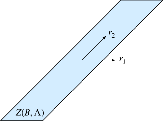
Figure 1: Solar penalty support set $Z(B,\Lambda)$ and its base vectors ($r_{1},r_{2}$).

The base representation of a solar penalty is a pair $(B,\Lambda)$ consisting of a tuple of unit vectors, $B=\lparen r_{1},\ldots,r_{m}\rparen$ which we call bases or base vectors, and a Cartesian product of closed intervals $\Lambda=I_{1}\times\cdots\times I_{m}$, where $I_{j}\subseteq[-\infty,\infty]$, $j=1,\ldots,m$, can possibly be unbounded. When convenient we may think of $B$ as being a matrix with unit norm columns. Then the solar penalty support set is

$$Z(B,\Lambda)\coloneqq B\cdot\Lambda=\bigg{\{}z\in\mathcal{X}\nonscript\>\bigg{|}\allowbreak\nonscript\>\mathopen{}z=\sum_{j=1}^{m}\lambda_{j}r_{j},\;\lambda_{j}\in I_{j}\bigg{\}}\,.$$

See Figure 1 for an example. The base representation of a solar penalty is useful, because it will allow us to connect $Z(B,\Lambda)$ to a reflection group (to be defined in Section 4.2) that encodes some of the geometry and symmetry of the penalty. Let us first discuss some examples for the case $\mathcal{X}=\mathbb{R}^{n}$.

Example 4.2 (Lasso).

Let $e_{j}$ denote the $j$th standard basis vector which has a $1$ in its $j$th coordinate and 0 elsewhere. The $\ell_{1}$ norm penalty has base representation

$$B =\big{\lparen}e_{1},\ldots,e_{n}\big{\rparen}$$

$$\Lambda =[-\lambda,\lambda]^{n}\,,$$

with $\lambda>0$. Then

$$Z(B,\Lambda)=\{z\in\mathbb{R}^{n}\nonscript\>|\allowbreak\nonscript\>\mathopen{}\lVert z\rVert_{\infty}\leq\lambda\}$$

and $h_{Z(B,\Lambda)}=\lVert\>\cdot\>\rVert_{1}$.

Example 4.3 (Nonnegative regression).

If we replace the intervals in the base representation of the $\ell_{1}$ penalty by the nonpositive half of the real line, then

$$B =\big{\lparen}e_{1},\ldots,e_{n}\big{\rparen}$$

$$\Lambda =[-\infty,0]^{n}\,,$$

and $Z(B,\Lambda)$ becomes the convex cone of vectors with nonpositive entries. The corresponding support function is the convex indicator of the nonnegative cone,

$$h_{Z(B,\Lambda)}(\theta)=\begin{cases}0&\text{if $\theta_{j}\geq 0$ for all $j$,}\\ +\infty&\text{otherwise.}\end{cases}$$

This is an example of a hard constraint. We could relax the constraint by replacing the intervals by

$$\Lambda=[-\lambda,0]^{n}\,.$$

In this case, the penalty operates like an $\ell_{1}$ norm on negative entries:

$$h_{Z(B,\Lambda)}(\theta)=\lambda\sum_{j}\lvert\min(0,\theta_{j})\rvert\,.$$

Example 4.4 (Fused lasso).

The 1d fused lasso is the $\ell_{1}$ norm of the first differences. This penalty is often used for smoothing and signal approximation when the data follow a one-dimensional structure. It encourages estimates that are piecewise constant. A base representation of this penalty is given by

$$B =\big{\lparen}(e_{j+1}-e_{j})/\sqrt{2}\nonscript\>\big{|}\allowbreak\nonscript\>\mathopen{}j=1,\ldots,n-1\big{\rparen}$$

$$\Lambda =[-\lambda,\lambda]^{n-1}$$

Then

$$h_{Z(B,\Lambda)}(\theta)=\frac{\lambda}{\sqrt{2}}\sum_{j=1}^{n-1}\lvert\theta_{j+1}-\theta_{j}\rvert\,.$$

In the engineering and signal processing literature the penalty is also known as total variation and more often employed in the case of 2d signals such as images [26]. Both the 1d and 2d cases can be described succinctly by introducing an undirected graph on $[p]$ with edge set $\mathcal{E}\subseteq[p]^{2}$. The 1d fused lasso correponds to a chain graph, while the 2d case corresponds to a 2d grid. The base representation then becomes

$$B =\big{\lparen}(e_{j}-e_{i})/\sqrt{2}\nonscript\>\big{|}\allowbreak\nonscript\>\mathopen{}\{i,j\}\in\mathcal{E}\big{\rparen}$$

$$\Lambda =[-\lambda,\lambda]^{\lvert\mathcal{E}\rvert}\,.$$

This graph-guided fused lasso penalty encourages estimates that are piecewise constant across nodes of the graph.

Example 4.5 (Isotonic regression).

Isotonic regression applies to linearly ordered data when the goal is to produce a monotonic fit. There is a large literature on the subject and the book by [3] is a standard reference. As a solar penalty, the isotonicity constraint can be viewed as a mix of fused lasso with a nonnegativity constraint on the first differences. The base representation of the penalty is

$$B =\big{\lparen}(e_{j+1}-e_{j})/\sqrt{2}\nonscript\>\big{|}\allowbreak\nonscript\>\mathopen{}j=1,\ldots,n-1\big{\rparen}$$

$$\Lambda =[-\infty,0]^{n-1}\,,$$

and the corresponding support function is the convex indicator function of the monotone cone,

$$h_{Z(B,\Lambda)}(\theta)=\begin{cases}0&\text{if $\theta_{j+1}\geq\theta_{j}$ for all $j$,}\\ +\infty&\text{otherwise.}\end{cases}$$

Nearly-isotonic regression [29] relaxes the isotone constraint and can be viewed as an $\ell_{1}$ penalty on positive first differences. It is obtained by replacing the above intervals by ones of the form $[-\lambda,0]$. Similarly to the fused lasso, the neighborhood structure can generalized from a chain graph to an arbitrary graph by making the obvious modification to the base. Though this seems to make the more sense with trees so that a partial order can be maintained.

Example 4.6 (Trend filtering).

Our final example is $\ell_{1}$ trend filtering [18]. Like the fused lasso, trend filtering applies to data with an ordering structure, but it uses the second difference instead of the first difference. This encourages estimates that are piecewise linear. In the case of linearly ordered data, the base representation of the trend filtering penalty has the form,

$$B =\big{\lparen}(e_{j+2}-2e_{j+1}+e_{j})/\sqrt{6}\nonscript\>\big{|}\allowbreak\nonscript\>\mathopen{}j=1,\ldots,n-2\big{\rparen}$$

$$\Lambda =[-\lambda,\lambda]^{n-2}\,.$$

The corresponding support function is an $\ell_{1}$ norm of the second differences:

$$h_{Z(B,\Lambda)}(\theta)=\frac{\lambda}{\sqrt{6}}\sum_{j=1}^{n-2}\lvert(x_{j+2}-x_{j+1})-(x_{j+1}-x_{j})\rvert\,.$$

We can form new solar penalties by taking the union of bases of existing penalties. This is effectively the same as adding the respective support functions. For example, the sparse fused lasso is the sum of the lasso and fused lasso penalties. Most importantly, the class of solar penalties is closed under addition with a separable support function.

4.2 The reflection group associated with a solar penalty

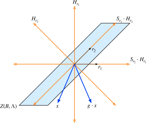
Figure 2: Reflection group $\mathcal{G}(B)$ associated with the solar penalty with base vectors ($r_{1},r_{2}$). The group is generated by two reflections, $S_{r_{1}}$ and $S_{r_{2}}$, across the hyperplanes $H_{r_{1}}$ and $H_{r_{2}}$. The remaining two hyperplanes are $S_{r_{1}}\cdot H_{r_{2}}$ and $S_{r_{2}}\cdot H_{r_{1}}$. The four hyperplanes partition the space into 8 chambers (cones) that the group acts transitively on.

The base vectors in the base representation of a solar penalty have a natural correspondence with hyperplanes in $\mathcal{X}$. Let $r\in\mathcal{X}$ be a unit vector and

$$H_{r}\coloneqq\{x\in\mathcal{X}\nonscript\>|\allowbreak\nonscript\>\mathopen{}\langle x,r\rangle=0\}\,.$$

$H_{r}$ is the hyperplane normal to $r$. The linear transformation $S_{r}:\mathcal{X}\to\mathcal{X}$ defined by $S_{r}\cdot x=x-2r\langle r,x\rangle$ is called the reflection across $H_{r}$ (or along $r$). Note that it satisfies

$$S_{r}\cdot r =-r$$

$$S_{r}\cdot H_{r} =H_{r}\,.$$

So it flips the sign of $r$ and leaves $H_{r}$ invariant. Associated to each solar penalty is a set of reflections $\{S_{r}\nonscript\>|\allowbreak\nonscript\>\mathopen{}r\in B\}$. These reflections generate a group of transformations.

Definition 4.7.

The reflection group generated by a set of base vectors $B$, denoted $\mathcal{G}(B)$, is the smallest closed subgroup of $\mathcal{O}(X)$ containing the set of reflections $\{S_{r}\nonscript\>|\allowbreak\nonscript\>\mathopen{}r\in B\}$.

See Figure 2 for an illustration. Note that although the group $\mathcal{G}(B)$ is finitely generated, it may be possible that $\mathcal{G}(B)$ is an infinite group. We will see later that this is the case for trend filtering. Table 1 lists the groups associated with each of the other example solar penalties discussed above. We will derive and discuss these in detail in Section 6, but first we return to the problem of reachability of the minimum norm element.

Group	Action	Penalty
$(\mathbb{Z}_{2})^{n}$	sign change	lasso, nonnegative regression
$\mathcal{P}_{n}$	permutation	fused lasso, isotonic regression
$(\mathbb{Z}_{2})^{n}\rtimes\mathcal{P}_{n}$	sign change and permutation	sparse fused lasso

Table 1: Some reflection groups, their action on $\mathcal{X}$, and associated solar penalties.

5 Existence of a polygonal path

To apply the general theory of Section 3 to solar penalized estimators we need to establish the existence of a $\mathcal{G}$-minimal element in the dual feasible set $x-Z(B,\Lambda)$ for some appropriate group. Theorem 3.4 tells us that the only candidate for a $\mathcal{G}$-minimal element is the minimum norm element. The following theorem shows that for a solar penalty, the reflection group generated by its base is an appropriate choice.

Theorem 5.1.

Let $(B,\Lambda)=(\lparen r_{1},\ldots,r_{m}\rparen,I_{1}\times\cdots\times I_{m})$ be the base representation of a solar penalty and $x\in\mathcal{X}$. If $\mathcal{G}\equiv\mathcal{G}(B)$ is the reflection group generated by $B$, then the minimum norm element of $x-Z(B,\Lambda)$ is $\mathcal{G}$-minimal in $x-Z(B,\Lambda)$.

The proof of Theorem 5.1 is similar in spirit to the path result of [13, page 47 ] [22, see] and its generalization by [10]. Let $y_{*}$ be the minimum norm element of $Z(B,\Lambda)$ and $y_{0}\in x-Z(B,\Lambda)$. We will construct a polygonal path from $y_{0}$ to $y_{*}$ where each segment along the path is obtained by averaging elementary transformations of the iterates. Our approach to constructing this path is algorithmic and was inspired by the boundary lemma proof of [30]. Consider applying cyclic coordinate descent to the minimum norm problem:

minimize $$\left\lVert x-{\textstyle\sum_{j=1}^{m}}\alpha_{j}r_{j}\right\rVert$$ (5.1)

subject to $$\alpha_{j}\in I_{j}\,,\quad j=1,\ldots,m\,.$$

Rather than tracking the iterates in terms of $(\alpha_{1},\ldots,\alpha_{m})$, we track them in terms of the fitted values,

$$y_{t}=x-\sum_{j}\alpha_{j}^{(t)}r_{j}\,,\quad t=0,1,2,\ldots\,.$$

A coordinate descent update modifies $y_{t}$ along one coordinate, say $j$, so that

$$y_{t+1}-y_{t}=\Big{\{}\alpha_{j}^{(t+1)}-\alpha_{j}^{(t)}\Big{\}}r_{j}\in\operatorname{span}(r_{j})\,.$$

So the selection of coordinate can instead be viewed as the selection of a base vector $r\in B$, and the update is find a minimum norm element along a line segment parallel to $r$. This yields the following geometric description of coordinate descent applied to 5.1.

1. Select the coordinate to be updated: $r\in B$.

2. Let $y_{t+1}$ be the minimum norm element in $(y_{t}+\operatorname{span}(r))\cap(x-Z(B,\Lambda))$.

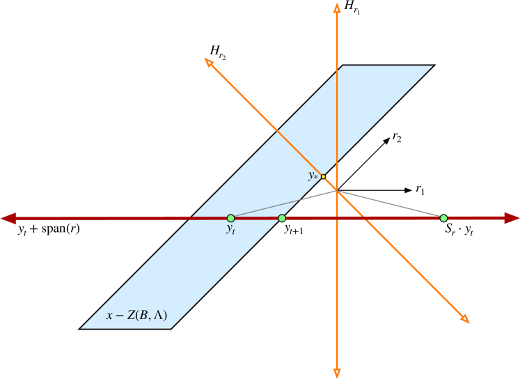
Figure 3: Coordinate descent update with $r=r_{1}$. The update moves $y_{t}$ to $y_{t+1}$ on a line parallel to $r$. The minimum norm point in $(y_{t}+\operatorname{span}(r))\cap(x-Z(B,\Lambda)$ is obtained by averaging $y_{t}$ with its reflection $S_{r}\cdot y_{t}$ across the hyperplane $H_{r}$.

Figure 3 illustrates the update, and it provides a visual explanation for the following lemma which we will use to prove Theorem 5.1.

Lemma 5.2.

Let $y_{0}\in x-Z(B,\Lambda)$ and $y_{t}$, $t=1,2,\ldots$, be the iterates of cyclic coordinate descent applied to the minimum norm problem 5.1. The iterates form a $\mathcal{G}$-monotone decreasing sequence with $\mathcal{G}\equiv G(B)$,

$$y_{t}\succeq_{\mathcal{G}}y_{t+1}\quad\text{for all}\quad t\,,$$

and $y_{t}\to y_{*}$, the minimum norm element of $x-Z(B,\Lambda)$, as $t\to\infty$.

Proof of Lemma 5.2.

[31, Theorem 4.1 ] establishes the convergence of $y_{t}$ to $y_{*}$, because the constraints of 5.1 are separable, the objective function is convex, and the lower level set $\{y\in\mathcal{X}\nonscript\>|\allowbreak\nonscript\>\mathopen{}\lVert y\rVert\leq\lVert y_{0}\rVert\}$ is compact. Moving on to the remaining claim, note that $y_{t}$, $S_{r}\cdot y_{t}$, and $y_{t+1}$ all lie on the line $y_{t}+\operatorname{span}(r)$. Since

$$\lVert y_{t+1}\rVert\leq\lVert y_{t}\rVert=\lVert S_{r}\cdot y_{t}\rVert\,,$$

the line segments $[0,y_{t}]$, $[0,S_{r}\cdot y_{t}]$ form the legs of an isoceles triangle with $y_{t+1}$ in the base of the triangle. It then follows that

$$y_{t+1}\in\operatorname{conv}\{y_{t},S_{r}\cdot y_{t}\}$$

and $y_{t+1}\preceq_{\mathcal{G}}y_{t}$ as desired. ∎

An interesting feature of this proof is that in the case of the permutation group, it shows that the coordinate descent update is an elementary Robin Hood operation [1]. More generally, the geometry of the coordinate descent updates is described by the reflection group. The iterates progress towards the minimum norm element by sequentially reflecting and averaging along each base vector, so the iterates must lie in $\operatorname{conv}(\mathcal{G}\cdot y_{0})$.

Proof of Theorem 5.1.

By induction, $y_{t}\in\operatorname{conv}(G\cdot y_{0})$. Since the orbitope is compact, $y_{*}\in\operatorname{conv}(G\cdot y_{0})$ and hence $y_{*}\preceq_{\mathcal{G}}y_{0}$ for all $y_{0}\in x-Z(B,\Lambda)$. ∎

6 Consequences

The immediate consequence of Theorem 5.1 is that the minimal norm element of the dual feasible set for the solar penalty is $\mathcal{G}$-minimal. Combining with Theorem 3.6 yields the main result of the paper:

Theorem 6.1.

Let $h_{C}$ be a solar penalty with base representation $(B,\Lambda)$ and $\mathcal{G}\equiv\mathcal{G}(B)$ be the reflection group generated by $B$. If $\mathcal{M}$ is a collection of expofam-type estimators with solar penalty $h_{C}$ and $\mathcal{G}$-invariant generators $\phi\in\Gamma_{0}(\mathcal{X})$ satisfying Assumption 3.5, then the penalized least squares estimator in $\mathcal{M}$ is computationally minimal for $\mathcal{M}$.

In the remainder of this section we will apply Theorem 6.1 in more detail to different families of estimators by taking the following steps.

1. Fix a solar penalty with base representation $(B,\Lambda)$.

2. Let $\mathcal{G}=\mathcal{G}(B)$ be the reflection group generated by $B$.

3. Let $\mathcal{M}$ be a collection of expofam-estimators with $\mathcal{G}$-invariant generators satisfying Assumption 3.5.

We will follow this program for each of the example solar penalties in Section 4 with $\mathcal{X}=\mathbb{R}^{n}$. The main challenge is identifying the reflection group.

6.1 Lasso and nonnegative regression

The base vectors of the $\ell_{1}$ norm are

$$B=\lparen e_{1},\ldots,e_{n}\rparen\,.$$

So the action of $S_{e_{j}}$ on $\mathbb{R}^{n}$ is simply to change the sign of the $j$th coordinate. Thus, $\mathcal{G}$ is isomorphic to the $n$-fold direct product of the cyclic group of order 2, $(\mathbb{Z}_{2})^{n}$. It then follows from Theorem 6.1 that

$$U(x)=\operatornamewithlimits{arg\,min}_{\theta}\frac{1}{2}\lVert x-\theta\rVert^{2}+\lambda\lVert\theta\rVert_{1}$$

is computationally minimal for all $\ell_{1}$-penalized expofam-type estimators with generators $\phi$ that depend only the magnitude of the coordinates of $\theta$. Since the nonnegative regression penalty has the same base as the $\ell_{1}$ norm, the same argument as above shows that

$$U(x)=\operatornamewithlimits{arg\,min}_{\theta\geq 0}\frac{1}{2}\lVert x-\theta\rVert^{2}$$

is computationally minimal for all nonnegative constrained expofam-type estimators with generators $\phi$ that depend only the magnitude of the coordinates of $\theta$. These two cases recover Examples 5 and 7 of [33].

6.2 Fused lasso/total variation and isotonic regression

The base vectors of the fused lasso penalty and isotonic regression are

$$B=\lparen(e_{j+1}-e_{j})/\sqrt{2}\nonscript\>|\allowbreak\nonscript\>\mathopen{}j=1,\ldots,n-1\rparen\,.$$

As a generator of a reflection group, this set is known as a fundamental system for the root system of the permutation group $\mathcal{P}_{n}$ [17, 36]. Another way to see this is to write out the reflection

$$S_{e_{j+1}-e_{j}}\,.$$

As a matrix it is equal to the identity everywhere except in the 2-by-2 submatrix for rows and columns $(j,j+1)$ where it has the form

$$\begin{bmatrix}0&1\\ 1&0\end{bmatrix}\,.$$

So the action of $S_{j}$ on $\mathbb{R}^{n}$ is the transposition $(j,j+1)$. It is well-known that these transpositions generate all permutations in $\mathcal{P}_{n}$. Then it follows from Theorem 6.1 that the least squares fused lasso (resp. isotonic regression) is computationally minimal for all total variation penalized (resp. isotonic regression) expofam-type estimators with permutation invariant generators.

Comparison with existing results

An instance of this phenomenon has already been pointed out in the literature. [2] considered generalized isotonic regression estimators of the form

minimize $$\sum_{j=1}^{n}[f(\theta_{j})-x_{j}\theta_{j}]w_{j}$$ (6.1)

subject to $$\theta_{1}\leq\theta_{2}\leq\cdots\leq\theta_{n}\,,$$

where $f$ is a proper convex function on $\mathbb{R}$ and $w_{j}>0$ are fixed weights. They showed that the solution to this problem could be obtained from the least squares solution with $f(u)=u^{2}/2$ [2, Theorem 3.1], i.e. that least squares is computationally minimal for generalized isotonic regression. There are two key differences with what we derived just now. 6.1 is an expofam-type estimator with generator of the form

$$\phi(\theta)=\sum_{j}f(\theta_{j})w_{j}\,.$$

This is a separable function and not necessarily permutation invariant unless the weights are constant. In constant weights case, this generator is permutation invariant, however our result allows possibly nonseparable permutation invariant functions.

[8] studied generalizations of total variation denoising solving problems of the form

minimize $$\sum_{j=1}^{n}f_{j}(\theta_{j})-x_{j}\theta_{j}+\lambda\sum_{j=1}^{n-1}\lvert\theta_{j+1}-\theta_{j}\rvert\,.$$ (6.2)

In the case where $f=f_{j}$, $j=1,\ldots,n$, is the log-partition of a one-dimensional exponential family they showed that the solution to 6.4 could be obtained from the least squares fit. This is a special case of our result with $\phi(\theta)=f(\theta_{1})+\cdots f(\theta_{n})$, which is clearly a permutation invariant function. Our result, however, does not require that the generator be separable.

Taut strings

There is a well-known connection between 1d total variation denoising and taut strings [21, 6]. Let $D_{n}:\mathbb{R}^{n}\to\mathbb{R}^{n-1}$ denote the first-difference operator on $\mathbb{R}^{n}$, i.e.

$$[D_{n}x]_{i}=x_{i+1}-x_{i}\,,\quad i=1,\ldots,n-1\,.$$

With some algebra, we can express the dual feasible set as

$$x-Z(B,\Lambda)=D_{n+1}\Sigma\,,$$ (6.3)

where

$$\Sigma=\left\{z\in\mathbb{R}^{n+1}\nonscript\>\middle|\allowbreak\nonscript\>\mathopen{}z_{1}=w_{1},z_{n+1}=w_{n+1},\lVert z-w\rVert_{\infty}\leq\lambda\right\}$$

and $w\in\mathbb{R}^{n+1}$ is the cumulative sum of $x$:

$$w_{i}=\sum_{j<i}x_{j}\,.$$

$\Sigma$ can be interpreted as a set of strings constrained to a tube of radius $\lambda$ centered at $y$. The end points of the string are fixed. The taut string problem is to find the string in $\Sigma$ of minimal length so that it is made taut:

minimize $$\sum_{j}\sqrt{1+(z_{j+1}-z_{j})^{2}}$$ (6.4)

subject to $$z\in\Sigma\,.$$

Using the identity 6.3, the taut string problem 6.4 can be written as

$$\min_{y\in x-Z(B,\Lambda)}\phi^{*}(y)\,,$$

where

$$\phi^{*}(y)=\sum_{j}\sqrt{1+y_{j}^{2}}$$

is permutation invariant convex function. Therefore, by Lemma 3.2 and Theorem 5.1, the taut string solution is given by the $\mathcal{G}$-minimal element of $x-Z(B,\Lambda)$ which is the same as least squares solution:

minimize $$\sum_{j}(z_{j+1}-z_{j})^{2}$$

subject to $$z\in\Sigma\,.$$

Additional insight can be gained by identifying the $\mathcal{G}$-majorization ordering. Since $\mathcal{G}$ is the permutation group, it is exactly the classical majorization ordering. So the taut string solution is the string with least majorized first difference.

Graph-guided versions

We conclude this example by pointing out that similar results hold for the graph fused lasso and graph isotonic regression.

Proposition 6.2.

If $\mathcal{E}$ is edge set of a connected undirected graph on $[n]$ and

$$B=\big{\lparen}(e_{j}-e_{i})/\sqrt{2}\nonscript\>\big{|}\allowbreak\nonscript\>\mathopen{}\{i,j\}\in\mathcal{E}\big{\rparen}\,,$$

then $\mathcal{G}(B)=\mathcal{P}_{n}$.

See Appendix A for the proof. A remarkable consequence of this observation is that the computational minimality phenomenon holds for the graph-guided fused lasso for as well.

Corollary 6.3.

Within the class of expofam-type estimators with fused lasso penalty (resp. isotonic regression) on a connected graph and permutation invariant generators $\phi\in\Gamma_{0}(\mathcal{X})$, the least squares estimator is computationally minimal.

If the graph is not connected, then it is not hard to see that the resulting reflection group is the direct product of permutation groups on nodes of each of the connected components. In other words, it is the subgroup of permutation generated by transpositions within each connected component. So the generators in the above corollary must invariant under permutations within those associated coordinates.

6.3 Sparse fused lasso

The sparse fused lasso penalty has the form

$$\lambda_{1}\sum_{j}\lvert\theta_{j}\rvert+\lambda_{2}\sum_{j}\lvert\theta_{j+1}-\theta_{j}\rvert\,.$$

It encourages both sparsity and smoothness in estimates of $\theta$. The base representation of this penalty has base vectors from the lasso and fused lasso penalties:

$$B=\big{\lparen}e_{1},\ldots,e_{n},(e_{2}-e_{1})/\sqrt{2},\ldots,(e_{n}-e_{n-1})/\sqrt{2}\big{\rparen}\,.$$

So $\mathcal{G}(B)$ must contain the reflection groups corresponding to the lasso and fused lasso as subgroups. The effect of the reflections in these subgroups on the standard basis are

$$S_{e_{j}}=\text{sign change on $e_{j}$}$$

and

$$S_{e_{j+1}-e_{j}}=\text{interchange of $e_{j}$ and $e_{j+1}$}\,.$$

So $\mathcal{G}(B)$ must be isomorphic to the semidirect product $(\mathbb{Z}_{2})^{n}\rtimes\mathcal{P}_{n}$ [17, 10], and it acts on $\mathbb{R}^{n}$ by sign change and permutations. Then by Theorem 6.1, among expofam-type estimators with a sparse fused lasso penalty and generators invariant under sign changes and permutations, the penalized least squares estimator is computationally minimal.

6.4 Trend filtering

Our next example is more of a nonexample. The base vectors of the trend filtering penalty are

$$B=\Big{\lparen}(e_{j+2}-2e_{j+1}+e_{j})/\sqrt{6}\nonscript\>\Big{|}\allowbreak\nonscript\>\mathopen{}j=1,\ldots,n-2\Big{\rparen}\,.$$

In an attempt to classify the group $\mathcal{G}(B)$ we compute the angle between pairs of base vectors. In this way we obtain the half-angle of rotation of the composition of pairs of reflections $S_{r_{i}}S_{r_{j}}$:

$$\arccos(\langle r_{i},r_{j}\rangle)=\begin{cases}0&\text{if $\lvert i-j\rvert=0$,}\\ \arccos(2/3)&\text{if $\lvert i-j\rvert=1$,}\\ \arccos(1/6)&\text{if $\lvert i-j\rvert=2$,}\\ \pi/2&\text{otherwise.}\end{cases}$$

Note that some of these angles are irrational multiples of $\pi$ [32], so the subgroups generated by each single rotation $S_{r_{i}}S_{r_{j}}$, $i=1$ or $i=2$, is of infinite order and isomorphic to the infinite dihedral group [7, 5]. Since $\mathcal{G}(B)\subseteq\mathcal{O}(\mathcal{X})$, perhaps the most practically useful statement we can make at the moment is that Theorem 6.1 is also true with $\mathcal{G}=\mathcal{O}(X)$. So least squares trend filtering is computationally minimal for the subcollection of expofam-type estimators with orthogonally invariant generators.

6.5 General solar penalties

As we have seen in the preceding examples, the reflection group generated by the base vectors $B=(r_{1},\ldots,r_{m})$ of a solar penalty depends on the arrangement of the hyperplanes $H_{r}$, $r\in B$. The resulting group $\mathcal{G}(B)$ may or may not be finite. The general theory of reflection groups is beyond the scope of this paper, but the book by [17] is great reference. In the case of trend filtering, $\mathcal{G}(B)$ failed to be finite because

$$\frac{1}{\pi}\arccos(\langle r_{i},r_{j}\rangle)=q_{ij}$$

was not rational for all $i,j$. We can easily verify that $q_{ij}$ is rational for all of the other examples. This is necessary and sufficient for $\mathcal{G}(B)$ to be a finite reflection group [17, see].

7 Discussion

Our main example explains within the computational sufficiency framework a deep explanation for phenomena discovered by [2] and [8] for isotonic regression and 1d total variation denoising, respectively. As we mentioned in the introduction, this has implications for both computation and inference. There is, however, some limits to what the existing theory can provide. Our final example of trend filtering showed that in some cases, the reflection group associated with a solar penalty may not have an easy interpretation. Nonetheless, we believe that the theory developed in this paper can have application beyond the examples considered. Here we suggest three possible directions for future research.

Extending to the generalized group lasso

An immediate question raised by this work is how to extend the results to generalized group lasso penalties. The use of the word “group” here refers to grouping of a variables as in the original group lasso paper [34]. This is important for the extension of fused lasso on a graph to multivariate observations and also for additive models [23, see, e.g.,]. One special case that has attracted much attention recently is the so-called convex fusion clustering [14, e.g.,] which is a convex relaxation of hierarchical clustering. One obvious way forward is to define a generalization of the solar penalty as a Minkowski sum of line segments, rays, and norm balls. Then most of the analysis in the paper should carry through, with block coordinate descent replacing coordinate descent. The main challenge will be finding a good notation system and identifying the corresponding groups.

Constructing solar penalties from a given reflection group

Rather than applying the theory to an existing generalized lasso penalty, we could instead start from some known reflection group for which we would like to maintain invariance. Section 6.5 suggests that we can construct a solar penalty by taking as base vectors the normal vectors of any generating set of reflections. This is related to concept of root systems and fundamental systems in the theory of reflection groups [17, see]. Alternatively, we could try to perturb the base vectors of trend filtering to obtain a more friendly group while still retaining desirable properties of trend filtering.

Exploiting group structure and geometry to develop efficient algorithms

The proof of Theorem 5.1 using dual coordinate descent suggests that the reflection group $\mathcal{G}(B)$ has an intrinsic role in iterative optimization. This is certainly the case for least squares regression problems. The optimality conditions for the dual problem involve normal cones of the dual feasible set $x-Z(B,\Lambda)$. These normal cones are related to the arrangement of hyperplanes corresponding to the base vectors and also to the Weyl chambers of the reflection group $\mathcal{G}(B)$. Is there a way to use this group structure and geometry to develop a more efficient algorithm for solving the dual problem?

Appendix A Additional proofs

A.1 Proof of Lemma 3.2

Proof.

$\text{\ref{case:g_minimal}}\implies\text{\ref{case:g_minimizes_convex_functions}}$: By Lemma 2.5,

$$f(z)\leq f(z)$$

for all $z\in K$. Then

$$f(z)\leq\inf_{z\in K}f(z)\,,$$

and we must have equality because $z\in K$.

$\text{\ref{case:g_minimizes_convex_functions}}\implies\text{\ref{case:g_minimal}}$: For any fixed $u\in\mathcal{X}$, the function

$$f_{u}(t) =h_{\mathcal{G}\cdot t}(u)$$

$$=\sup_{g\in\mathcal{G}}\langle g\cdot t,u\rangle$$

$$=\sup_{g\in\mathcal{G}}\langle t,g^{-1}\cdot u\rangle$$

is $\mathcal{G}$-invariant and convex, because it is the pointwise supremum of a family of convex functions [4, Proposition 8.16]. Then for $z\in K$,

$$h_{\mathcal{G}\cdot y}(u) =f_{u}(y)$$

$$=\inf_{w\in K}f_{u}(w)$$

$$\leq f_{u}(z)=h_{\mathcal{G}\cdot z}(u)\,,$$

and by Lemma 2.5, $y\preceq_{\mathcal{G}}z$. ∎

A.2 Proof of Lemma 3.3

Proof.

(a): This is trivial.

(b): By Lemma 2.5, if $y\preceq_{\mathcal{H}}z$, then

$$y\in\operatorname{conv}(\mathcal{H}\cdot y)\subseteq\operatorname{conv}(\mathcal{G}\cdot z)$$

and $y\preceq_{\mathcal{G}}z$.

(c): It is easy to see that $y\preceq_{\mathcal{O}(\mathcal{X})}y$ if and only if $\lVert y\rVert\leq\lVert z\rVert$. So $y$ is $\mathcal{O}(\mathcal{X})$-minimal in $K$ if and only if

$$\lVert y\rVert=\inf_{z\in K}\lVert z\rVert\,.$$

Since $K$ is closed and convex, such an element exists uniquely.

(d): By (b) and (c), if $y$ is $\mathcal{G}$-minimal in $K$, then it must be the unique $\mathcal{O}(\mathcal{X})$-minimal element of $K$, which, as shown above, is the minimum norm element. ∎

A.3 Proof of Theorem 3.6

Proof.

We will prove the following claims:

1. $U(x)$ is $\mathcal{G}$-minimal in $x-C$,

2. $U(x)$ is dual optimal for every $T\in\mathcal{M}$

3. 3.2 recovers the primal solutions, and

4. $U\in\mathcal{M}$.

Claim (1)

This is immediate from Theorem 3.4.

Claim (2)

Let $x\in\mathcal{X}$, $y_{*}=U(x)$, and fix $T\in\mathcal{M}$ with generator $\phi$. The dual problem to $T(x)$ is

$$-\min_{y\in x-C}\phi^{*}(y)\,.$$

Note that $\phi^{*}$ is $\mathcal{G}$-invariant and convex. If this dual problem has a solution, then it follows from the $\mathcal{G}$-minimality of $y_{*}$ in $x-C$ that $y_{*}$ is a solution.

Claim (3)

Assumption 3.5 ensures that strong duality holds so that a primal and dual solution pair $(\theta,x-z)$ are related by the equations

$$x-z \in\partial\phi(\theta)$$

$$\theta \in N_{C}(z)\,.$$

This in turn is equivalent to

$$\langle x-z,\theta\rangle =\phi^{*}(x-z)+\phi(\theta)$$

$$\langle z,\theta\rangle =h_{C}(\theta)\,.$$

Thus,

$$T(x)=\operatornamewithlimits{arg\,min}_{\theta}\phi(\theta)-\langle y,\theta\rangle+h_{C}(\theta)\,.$$

for any dual solution $y$. Conversely, if $T(x)$ is nonempty then a dual solution exists, and by Claims 1 and 2, $y_{*}$ is a dual solution and 3.2 holds.

Claim (4)

Let $\phi=\frac{1}{2}\lVert\>\cdot\>\rVert^{2}$. Assumption 3.5 holds in this case and $\phi$ is $\mathcal{G}$-invariant, because $\mathcal{G}\subseteq\mathcal{O}(X)$. Then by applying 3.2,

$$\operatornamewithlimits{arg\,min}_{\theta}\phi(\theta)-\langle U(x),\theta\rangle=\operatornamewithlimits{arg\,min}_{\theta}\frac{1}{2}\lVert\theta-U(x)\rVert^{2}=U(x)\,.$$

So $U\in\mathcal{M}$ is computationally necessary and hence computationally minimal. ∎

A.4 Proof of Proposition 6.2

Proof.

The reflections associated with $B$ are transpositions of the form $(i,j)\in\mathcal{E}$. Since the graph is connected, between any pair of vertices, say $u,v$, there exists a path. Then the product of the transpositions of the edges along the graph, taken in order from $u$ to $v$, is simply the transposition $(u,v)$. For example,

$$(u,i_{1})(i_{1},i_{2})(i_{2},v)=(u,i_{2})(i_{2},v)=(u,v)\,.$$

Since $\mathcal{G}(B)$ contains all transpositions it must be $\mathcal{P}_{n}$. ∎

References

- [1] Barry C Arnold and José Marı́a Sarabia “Majorization and the Lorenz Order with Applications in Applied Mathematics and Economics” Springer, 2018
- [2] R.. Barlow and H.. Brunk “The Isotonic Regression Problem and Its Dual” In Journal of the American Statistical Association 67.337 [American Statistical Association, Taylor & Francis, Ltd.], 1972, pp. 140–147 DOI: 10.2307/2284712
- [3] Richard E. Barlow, D.J. Bartholomew, J.. Bremner and H.. Brunk “Statistical Inference Under Order Restrictions: Theory and Application of Isotonic Regression (Probability & Mathematical Statistics)” John Wiley & Sons Ltd, 1972
- [4] Heinz H. Bauschke and Patrick L. Combettes “Convex Analysis and Monotone Operator Theory in Hilbert Spaces” Springer New York, 2017 DOI: 10.1007/978-3-319-48311-5
- [5] L. Condat “A Direct Algorithm for 1-D Total Variation Denoising” In IEEE Signal Processing Letters 20.11, 2013, pp. 1054–1057 DOI: 10.1109/LSP.2013.2278339
- [6] P.. Davies and A. Kovac “Local Extremes, Runs, Strings and Multiresolution” In Annals of statistics 29.1 Institute of Mathematical Statistics, 2001, pp. 1–65 DOI: 10.1214/aos/996986501
- [7] Igor Dolgachev “Reflection groups in algebraic geometry” In Bulletin of the American Mathematical Society 45.1, 2008, pp. 1–60 URL: https://www.ams.org/journals/bull/2008-45-01/S0273-0979-07-01190-1/S0273-0979-07-01190-1.pdf
- [8] Lutz Dümbgen and Arne Kovac “Extensions of smoothing via taut strings” In Electronic journal of statistics 3 The Institute of Mathematical Statisticsthe Bernoulli Society, 2009, pp. 41–75 DOI: 10.1214/08-EJS216
- [9] Morris L. Eaton “On group induced orderings, monotone functions, and convolution theorems” In Inequalities in Statistics and Probability Institute of Mathematical Statistics, 1984, pp. 13–25 DOI: 10.1214/lnms/1215465625
- [10] Morris L. Eaton and Michael D. Perlman “Reflection Groups, Generalized Schur Functions, and the Geometry of Majorization” In Annals of Probability 5.6 Institute of Mathematical Statistics, 1977, pp. 829–860 DOI: 10.1214/aop/1176995655
- [11] Andrew R. Francis and Henry P. Wynn “Subgroup majorization” In Linear algebra and its applications 444, 2014, pp. 53–66 DOI: 10.1016/j.laa.2013.11.042
- [12] A. Giovagnoli and H.. Wynn “G-majorization with applications to matrix orderings” In Linear algebra and its applications 67, 1985, pp. 111–135 DOI: 10.1016/0024-3795(85)90190-9
- [13] Godfrey Harold Hardy, John Edensor Littlewood and George Pólya “Inequalities” Cambridge University Press, 1988
- [14] Toby Dylan Hocking, Armand Joulin, Francis Bach and Jean-Philippe Vert “Clusterpath an algorithm for clustering using convex fusion penalties” In 28th International Conference on Machine Learning, 2011 URL: https://www.di.ens.fr/~fbach/419_icmlpaper.pdf
- [15] Holger Höfling “A Path Algorithm for the Fused Lasso Signal Approximator” In Journal of computational and graphical statistics: a joint publication of American Statistical Association, Institute of Mathematical Statistics, Interface Foundation of North America 19.4 Taylor & Francis, 2010, pp. 984–1006 DOI: 10.1198/jcgs.2010.09208
- [16] Nicholas A. Johnson “A Dynamic Programming Algorithm for the Fused Lasso and L 0-Segmentation” In Journal of computational and graphical statistics: a joint publication of American Statistical Association, Institute of Mathematical Statistics, Interface Foundation of North America 22.2 Taylor & Francis, 2013, pp. 246–260 DOI: 10.1080/10618600.2012.681238
- [17] Richard Kane “Reflection groups and invariant theory” Springer Science & Business Media, 2013
- [18] S. Kim, K. Koh, S. Boyd and D. Gorinevsky “ Trend Filtering” In SIAM Review 51.2 Society for IndustrialApplied Mathematics, 2009, pp. 339–360 DOI: 10.1137/070690274
- [19] Céline Levy-Leduc and Zaïd Harchaoui “Catching Change-points with Lasso” In Advances in Neural Information Processing Systems 20 Curran Associates, Inc., 2008, pp. 617–624 URL: http://papers.nips.cc/paper/3188-catching-change-points-with-lasso.pdf
- [20] Kevin Lin, James L. Sharpnack, Alessandro Rinaldo and Ryan J. Tibshirani “A Sharp Error Analysis for the Fused Lasso, with Application to Approximate Changepoint Screening” In Advances in Neural Information Processing Systems 30 Curran Associates, Inc., 2017, pp. 6884–6893 URL: http://papers.nips.cc/paper/7264-a-sharp-error-analysis-for-the-fused-lasso-with-application-to-approximate-changepoint-screening.pdf
- [21] Enno Mammen and Sara van de Geer “Locally adaptive regression splines” In Annals of statistics 25.1, 1997, pp. 387–413 DOI: 10.1214/aos/1034276635
- [22] Albert W Marshall, Ingram Olkin and Barry C Arnold “Inequalities: theory of majorization and its applications” Springer, 2011
- [23] Ashley Petersen, Daniela Witten and Noah Simon “Fused Lasso Additive Model” In Journal of computational and graphical statistics: a joint publication of American Statistical Association, Institute of Mathematical Statistics, Interface Foundation of North America 25.4 Taylor & Francis, 2016, pp. 1005–1025 DOI: 10.1080/10618600.2015.1073155
- [24] Alessandro Rinaldo “Properties and Refinements of the Fused Lasso” In Annals of statistics 37.5B Institute of Mathematical Statistics, 2009, pp. 2922–2952 URL: http://www.jstor.org/stable/30243732
- [25] Cristian R. Rojas and Bo Wahlberg “On change point detection using the fused lasso method” In arXiv [math.ST], 2014 URL: http://arxiv.org/abs/1401.5408
- [26] Leonid I. Rudin, Stanley Osher and Emad Fatemi “Nonlinear total variation based noise removal algorithms” In Physica D. Nonlinear phenomena 60.1, 1992, pp. 259–268 DOI: 10.1016/0167-2789(92)90242-F
- [27] A… Steerneman “G-Majorization, group-induced cone orderings, and reflection groups” In Linear algebra and its applications 127, 1990, pp. 107–119 DOI: 10.1016/0024-3795(90)90338-D
- [28] Robert Tibshirani, Michael Saunders, Saharon Rosset, Ji Zhu and Keith Knight “Sparsity and smoothness via the fused lasso” In Journal of the Royal Statistical Society. Series B, Statistical methodology 67.1, 2005, pp. 91–108 DOI: 10.1111/j.1467-9868.2005.00490.x
- [29] Ryan J. Tibshirani, Holger Höfling and Robert Tibshirani “Nearly-Isotonic Regression” In Technometrics: a journal of statistics for the physical, chemical, and engineering sciences 53.1 Taylor & Francis, Ltd., 2011, pp. 54–61 URL: http://www.jstor.org/stable/40997292
- [30] Ryan J. Tibshirani and Jonathan Taylor “The solution path of the generalized lasso” In Annals of statistics 39.3 Institute of Mathematical Statistics, 2011, pp. 1335–1371 DOI: 10.1214/11-AOS878
- [31] P. Tseng “Convergence of a Block Coordinate Descent Method for Nondifferentiable Minimization” In Journal of optimization theory and applications 109.3, 2001, pp. 475–494 DOI: 10.1023/A:1017501703105
- [32] Juan L. Varona “Rational values of the arccosine function” In Central European Journal of Mathematics 4.2 Walter de Gruyter GmbH, 2006, pp. 319–322 DOI: 10.2478/s11533-006-0011-z
- [33] Vincent Q. Vu “Group Invariance and Computational Sufficiency”, 2018 arXiv:1807.05985
- [34] Ming Yuan and Yi Lin “Model selection and estimation in regression with grouped variables” In Journal of the Royal Statistical Society. Series B, Statistical methodology 68.1, 2006, pp. 49–67 DOI: 10.1111/j.1467-9868.2005.00532.x
- [35] Günter M Ziegler “Lectures on polytopes” Springer Science & Business Media, 2012